Approximations of Metric Graphs by Thick Graphs and Their Laplacians

Abstract

The main purpose of this article is two-fold: first, to justify the choice of Kirchhoff vertex conditions on a metric graph as they appear naturally as a limit of Neumann Laplacians on a family of open sets shrinking to the metric graph (“thick graphs”) in a self-contained presentation; second, to show that the metric graph example is close to a physically more realistic model where the edges have a thin, but positive thickness. The tool used is a generalization of norm resolvent convergence to the case when the underlying spaces vary. Finally, we give some hints about how to extend these convergence results to some mild non-linear operators.

1. Introduction

The study of operators on metric graphs has been an ongoing and active area of research for at least two decades. Several natural questions arise in the study of Laplacians on metric graphs: As there is some freedom in defining a self-adjoint Laplacian on a metric graph due to the vertex conditions (see, e.g., [1] and the references therein), can one justify a certain choice of such vertex conditions? Second, in a realistic physical model (a thick graph), the wires have a thickness of order $\epsilon$, but in the metric graph model, it is simplified to $\epsilon =0$: Can one justify some sort of limit of a Laplacian on the network with thickness $\epsilon >0$ as $\epsilon \to 0$?

The aim of this article is to give an answer to both questions. We show that the Neumann Laplacian on the $\epsilon$-neighborhood of the metric graph (embedded in some ambient space ${\mathbb{R}}^{m+1}$) converges to the Kirchhoff Laplacian on the metric graph. This gives answers to both questions above: First, the “natural” vertex conditions are the so-called Kirchhoff conditions; see Equations (3) and (4). Second, the limit problem is a good approximation to a realistic physical model on a thick graph as $\epsilon \to 0$. Note that the problem significantly simplifies in the limit, as we only have to consider a system of ODEs instead of a PDE on a complicated and $\epsilon$-dependent space. Moreover, the problem on the metric graph can often be solved explicitly.

A technical difficulty is that the Laplacian on the thick graph and on the metric graph live on different spaces. We therefore generalize the notion of norm resolvent convergence to this case; this was first done in [2]; see also the monograph [3] for a history of the problem and [4] for a recent list of references. Convergence of the (discrete) spectrum for the Neumann Laplacian on a thick graph converging to a compact metric graph has already been established by variational methods in [5,6,7].

The aim of this article is also to provide an almost self-contained presentation of the results for linear operators on thick and metric graphs to the “non-linear” community and also to give some ideas of how they can be extended to some mild non-linear operators.

2. Metric Graphs and Their Laplacians

For a detailed presentation of metric graphs and their Laplacians, we refer to [1,3] and the references therein. Let $X_0$ denote a metric graph given by the data $(V,E,\ell )$, where V and E are the (at most countable) sets of vertices and edges, respectively, and where $\ell :E⟶(0,\infty )$. $e\mapsto {\ell }_e$ denotes the length of the edge $e\in E$; a metric edge will be the interval $I_e:=[0,{\ell }_e]$. The metric graph $X_0$ is now the disjoint union of all metric edges ${error}_{e\in E}{I}_e$ after identifying the endpoints $\partial I_e$ with the corresponding vertices. A metric graph is a metric space using the intrinsic metric (i.e., $d(s,\tilde{s})$ is the length of the shortest path in $X_0$ between s and $\tilde{s}$). Moreover, there is a natural measure on $X_0$ given by the sum of the Lebesgue measures on each metric edge $I_e$.

As the Hilbert space on $X_0$, we choose:

$${\mathcal{H}}_0:={\mathsf{L}}_2^{}\left(X_0\right)=\underset{e\in E}{⨁}{\mathsf{L}}_2^{}\left(I_e\right),$$

where we write $f\in {\mathsf{L}}_2^{}\left(X_0\right)$ as family ${\left(f_e\right)}_{e\in E}$ with $f_e\in {\mathsf{L}}_2^{}\left(I_e\right)$; moreover, ${⨁}_{e\in E}{\mathsf{L}}_2^{}\left(I_e\right)$ denotes the Hilbert orthogonal sum with f being in it if its squared norm:

$${\parallel f\parallel }_{{\mathsf{L}}_2^{}\left(X_0\right)}^2:=\sum _{e\in E}{\int }_{I_e}{\left|f_e\left(s\right)\right|}_{}^2\mathrm{d}s$$

is finite. Similarly, we define ${\mathsf{H}}_{\mathrm{dec}}^k\left(X\right):={⨁}_{\mathrm{e}\in E}{\mathsf{H}}^k\left(I_e\right)$ for $k\in {\mathbb{N}}_0$. The label “$\mathrm{dec}$” refers to the fact that for $k\ge 1$, there is no relation between the (well-defined) values of $f_e$ and its derivatives at a vertex v for different $e\in E_v$. Here, $E_v$ denotes the set of edges that are adjacent with the vertex $v\in V$. Recall that functions in ${\mathsf{H}}^1\left(I_e\right)$ are continuous as we have the estimate:

$${\left|f_e\left(s\right)-f_e\left(\tilde{s}\right)\right|}_{}^2\le \left|s-\tilde{s}\right|{\int }_{I_e}{\left|f_e^{\prime }\left(u\right)\right|}_{}^2\mathrm{d}u.$$

Using a suitable cut-off function, we conclude the Sobolev trace estimate:

$${\left|f_e\left(v\right)\right|}_{}^2\le C_e{\parallel f_e\parallel }_{{\mathsf{H}}^1\left(I_e\right)}=C_e{\int }_{I_e}\left({\left|f_e\left(s\right)\right|}_{}^2+{\left|f_e^{\prime }\left(s\right)\right|}_{}^2\right)\mathrm{d}s$$

(1)

with $C_e=2/min\{1,{\ell }_e\}$, where $f_e\left(v\right)$ denotes the evaluation of $f_e$ at one of the endpoints of $I_e$ corresponding to $v\in V$. In particular, we assume that:

$${\ell }_0:=min\{\underset{e\in E}{inf}{\ell }_e,1\}>0.$$

(2)

From (1) and (2), we then conclude that the subspace:

$${\mathsf{H}}^1\left(X_0\right):={\mathsf{H}}_{\mathrm{dec}}^1\left(X_0\right)\cap {\mathsf{C}}^{}\left(X_0\right)=\left\{f\in {\mathsf{H}}_{\mathrm{dec}}^1\left(X_0\right)f_e\left(v\right)\mathrm{is}\mathrm{independent}\mathrm{of}e\in E_v\mathrm{for}\mathrm{all}v\in V\right\}$$

(3)

is closed in ${\mathsf{H}}_{\mathrm{dec}}^1\left(X_0\right)$. We denote by $f\left(v\right):=f_e\left(v\right)$ the common value of f at the vertex v. It follows that:

$${\mathfrak{l}}_0\left(f\right):={\parallel f^{\prime }\parallel }_{}^2=\sum _{e\in E}{\int }_{I_e}{\left|f_e^{\prime }\left(s\right)\right|}_{}^2\mathrm{d}s,f\in dom{\mathfrak{l}}_0:={\mathsf{H}}^1\left(X_0\right),$$

defines a closed, non-negative quadratic form in ${\mathcal{H}}_0={\mathsf{L}}_2^{}\left(X_0\right)$. The associated self-adjoint and non-negative operator $L_0$ is given by:

$${\left(L_{0}f\right)}_e=-f_e^{″},f\in dom{L}_0=\left\{f\in {\mathsf{H}}_{\mathrm{dec}}^2\left(X_0\right)|f\in {\mathsf{C}}^{}\left(X_0\right),\sum _{e\in E_v}{f}_e^{\prime }\left(v\right)=0\right\}.$$

(4)

Here, $f_e^{\prime }\left(v\right)$ denotes the (weak) derivative of $f_e$ along e towards the vertex v. The operator $L_0$ is sometimes referred to as the (generalized) Neumann Laplacian or Kirchhoff Laplacian (the second because of the flux condition ${\sum }_{e\in E_v}{f}_e^{\prime }\left(v\right)=0$ on the derivatives). Note that for vertices of degree one, the vertex condition is just the usual Neumann boundary condition $f_e^{\prime }\left(v\right)=0$, and for vertices of degree two, we have $f_{e_1}\left(v\right)=f_{e_2}\left(v\right)$ and $f_{e_1}^{\prime }\left(v\right)+f_{e_2}^{\prime }\left(v\right)=0$, i.e., the continuity of f and its derivative along v (recall that $f_e^{\prime }\left(v\right)$ denotes the derivative towards the vertex v).

3. Thick Graphs and Their Laplacians

We assume first that the metric graph $X_0$ is embedded in some space ${\mathbb{R}}^{m+1}$ ($m\ge 1$) such that all edges are straight line segments in ${\mathbb{R}}^{m+1}$. For $\epsilon >0$, denote by:

$$X_{\epsilon }^{\diamond }:=\left\{x\in {\mathbb{R}}^{m+1}|d(x,X_0)<\epsilon /{\omega }_m\right\}$$

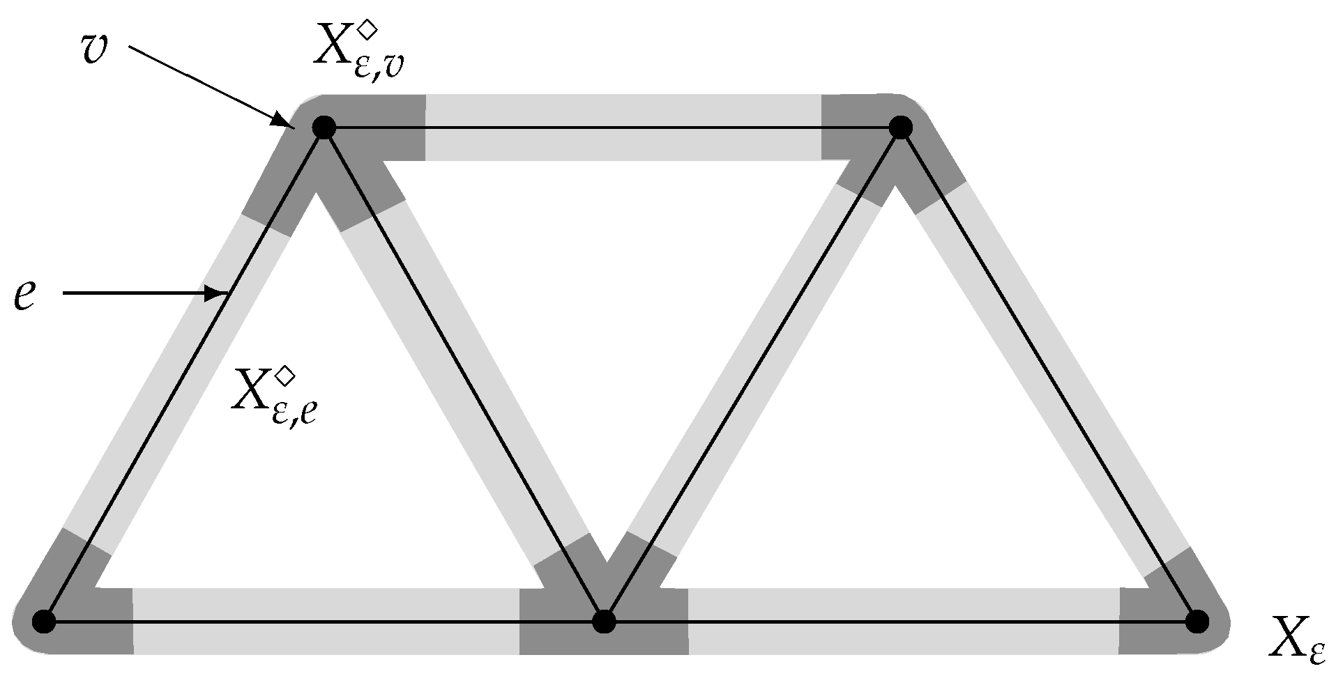
the $\epsilon /{\omega }_m$-neighborhood of $X_0$ in ${\mathbb{R}}^{m+1}$. Here, ${\omega }_m$ is the mth root of the volume of the unit Euclidean ball in ${\mathbb{R}}^m$, i.e., ${\omega }_1=2$, ${\omega }_2=\sqrt{\pi }$, ${\omega }_3=\sqrt[3]{4\pi /3}$, etc. We say that $X_{\epsilon }^{\diamond }$ is a graph-like space or a thick graph constructed from the metric graph $X_0$ if there is ${\epsilon }_0>0$ such that:

$${\overline{X_{\epsilon }^{\diamond }}}^{}=\bigcup _{v\in V}{\overline{X_{\epsilon ,v}^{\diamond }}}^{}\cup \bigcup _{e\in E}{\overline{X_{\epsilon ,e}^{\diamond }}}^{}$$

(5)

for all $\epsilon \in (0,{\epsilon }_0]$ (cf. Figure 1), where $X_{\epsilon ,v}^{\diamond }$ and $X_{\epsilon ,e}^{\diamond }$ are open and pairwise disjoint subsets of ${\mathbb{R}}^{m+1}$ such that the so-called vertex and edge neighborhoods fulfil:

$$X_{\epsilon ,v}^{\diamond }\cong \epsilon X_v\mathrm{and}{X}_{\epsilon ,e}^{\diamond }\cong \left(\epsilon ,{\ell }_e-2a_e\epsilon \right)\times \epsilon B,$$

(6)

i.e., $X_{\epsilon ,v}^{\diamond }$ is isometric to the $\epsilon$-scaled version of an open subset $X_v$, $X_{\epsilon ,e}^{\diamond }$ is isometric with the product of an interval of length ${\ell }_e-2a_e\epsilon$, and $B\subset {\mathbb{R}}^m$ is a ball of radius $1/{\omega }_m$, having m-dimensional volume one by the definition of the scaling factor ${\omega }_m$. Moreover, $2a_e\epsilon$ is the sum of the lengths of the two parts of the metric edge inside the vertex neighborhood. For finite graphs, the existence of ${\epsilon }_0>0$ is no restriction, but for infinite graphs with an arbitrary large vertex degree, this might be a restriction on the embedding and the edge lengths. More details on spaces constructed according to a graph (so-called “graph-like spaces”) can be found in the monograph [3]; see also the references therein.

As the Hilbert space, we set ${\mathcal{H}}_{\epsilon }^{\diamond }:={\mathsf{L}}_2^{}\left(X_{\epsilon }^{\diamond }\right)$. As the operator, we use the (non-negative) Neumann Laplacian $L_{\epsilon }^{\diamond }$ defined as the self-adjoint and non-negative operator associated with the closed and non-negative quadratic form given by:

$${\mathfrak{a}}_{\epsilon }^{\diamond }\left(u\right):={\parallel \nabla u\parallel }_{{\mathsf{L}}_2^{}\left(X_{\epsilon }^{\diamond }\right)}^2$$

in ${\mathcal{H}}_{\epsilon }^{\diamond }={\mathsf{L}}_2^{}\left(X_{\epsilon }^{\diamond }\right)$.

In our calculations later, it is more convenient to work with edge neighborhoods $X_{\epsilon ,e}$ that are isometric with the product of the original edge $I_e$ times the $\epsilon$-scaled ball B, i.e.,

$$X_{\epsilon ,e}\cong I_e\times \epsilon B$$

instead of the slightly shortened edge neighborhood $X_{\epsilon ,e}^{\diamond }$. For $v\in V$, we set $X_{\epsilon ,v}=X_{\epsilon ,v}^{\diamond }=\epsilon X_v$. We then construct $X_{\epsilon }$ as the space obtained from gluing the building blocks $X_{\epsilon ,v}$ and $X_{\epsilon ,e}$ such that a decomposition similar to (5) holds, now without the label ${(·)}^{\diamond }$. Note that $X_{\epsilon }$ is defined as an abstract flat manifold with boundary and might not be embeddable into ${\mathbb{R}}^{m+1}$ any longer. We also call $X_{\epsilon }$ a graph-like space or thick graph. We state that the Neumann Laplacians on $X_{\epsilon }$ and $X_{\epsilon }^{\diamond }$ are “close to each other” in Lemma 4.

Due to a decomposition of $X_{\epsilon }$ into its building blocks similar to (5) and the scaling behavior, the norm in the Hilbert space ${\mathcal{H}}_{\epsilon }:={\mathsf{L}}_2^{}\left(X_{\epsilon }\right)$ fulfills:

$${\parallel u\parallel }_{{\mathsf{L}}_2^{}\left(X_{\epsilon }\right)}^2=\sum _{v\in V}{\epsilon }^{m+1}{\int }_{X_v}{\left|u_v\left(x\right)\right|}_{}^2\mathrm{d}x+\sum _{e\in E}{\epsilon }^m{\int }_{I_e}{\int }_B{\left|u_e(s,y)\right|}_{}^2\mathrm{d}y\mathrm{d}s,$$

where $u_v$ and $u_e$ denote the restriction of u onto the $\epsilon$-independent building blocks $X_v$ and $X_e=I_e\times B$. Note that with this notation, we have put all $\epsilon$-dependencies into the norm (and later also into the quadratic form).

As the operator, we use the (negative) Neumann Laplacian $L_{\epsilon }$ defined as the self-adjoint and non-negative operator associated with the closed and non-negative quadratic form given by:

$$\begin{array}{cc}\hfill {\mathfrak{l}}_{\epsilon }\left(u\right):=& {\parallel \nabla u\parallel }_{{\mathsf{L}}_2^{}\left(X_{\epsilon }\right)}^2\hfill \\ \hfill =& \sum _{v\in V}{\epsilon }^{m-1}{\int }_{X_v}{\left|\nabla u_v\left(x\right)\right|}_{}^2\mathrm{d}x+\sum _{e\in E}{\epsilon }^m{\int }_{I_e}{\int }_B\left({\left|u_e^{\prime }(s,y)\right|}_{}^2+\frac{1}{{\epsilon }^2}{\left|{\nabla }_B{u}_e(s,y)\right|}_{}^2\right)\mathrm{d}y\mathrm{d}s\hfill \end{array}$$

in ${\mathcal{H}}_{\epsilon }={\mathsf{L}}_2^{}\left(X_{\epsilon }\right)$ using the scaling behavior of the building blocks. Here, $u_e^{\prime }$ denotes the derivative with respect to the longitudinal (first) variable s, and ${\nabla }_B$ denotes the derivative with respect to the second variable $y\in B$.

4. Convergence of the Resolvents

How can we now compare the two Laplacians $L_0$ and $L_{\epsilon }$ (resp. $L_{\epsilon }^{\diamond }$)? The idea is first to consider the resolvents:

$$R_0:={(L_0+1)}^{-1}\mathrm{resp}.R_{\epsilon }:={(L_{\epsilon }+1)}^{-1}$$

in ${\mathcal{H}}_0$, resp. ${\mathcal{H}}_{\epsilon }$, since they are bounded operators. In order to define a norm difference of these resolvents, we need a so-called identification operator:

$$J_{\epsilon }:{\mathcal{H}}_0⟶{\mathcal{H}}_{\epsilon },$$

in our situation given by

$${\left(J_{\epsilon }f\right)}_v=0\mathrm{and}{\left(J_{\epsilon }f\right)}_e(s,y)={\epsilon }^{-m/2}{f}_e\left(s\right),$$

i.e., we set $Jf$ to zero on the vertex neighborhood and transversally constant on the edge neighborhood, together with an appropriate rescaling constant. As the identification operator in the opposite direction, we use $J_{\epsilon }^{*}:{\mathcal{H}}_{\epsilon }⟶{\mathcal{H}}_0$, where an easy calculation shows that:

$${\left(J_{\epsilon }^{*}u\right)}_e\left(s\right)={\epsilon }^{m/2}{\int }_B{u}_e(s,y)\mathrm{d}y.$$

It is easy to see that $J_{\epsilon }^{*}{J}_{\epsilon }f=f$, i.e., $J_{\epsilon }$ is an isometry.

We now compare the two resolvents, sandwiched with $J_{\epsilon }$. Let:

$$D_{\epsilon }:=R_{\epsilon }{J}_{\epsilon }-J_{\epsilon }{R}_0:{\mathcal{H}}_0⟶{\mathcal{H}}_{\epsilon }.$$

What does $D_{\epsilon }$ look like? The best way to deal with it is to consider ${\langle D_{\epsilon }g,w\rangle }_{{\mathcal{H}}_{\epsilon }}$ for $g\in {\mathcal{H}}_0$ and $w\in {\mathcal{H}}_{\epsilon }$. We have:

$$\begin{array}{cc}{\langle D_{\epsilon }g,w\rangle }_{{\mathcal{H}}_{\epsilon }}\hfill & ={\langle J_{\epsilon }g,R_{\epsilon }w\rangle }_{{\mathcal{H}}_{\epsilon }}-{\langle J_{\epsilon }{R}_{0}g,w\rangle }_{{\mathcal{H}}_{\epsilon }}\hfill \\ & ={\langle J_{\epsilon }{L}_{0}f,u\rangle }_{{\mathcal{H}}_{\epsilon }}-{\langle J_{\epsilon }f,L_{\epsilon }u\rangle }_{{\mathcal{H}}_{\epsilon }},\hfill \end{array}$$

where $u=R_{\epsilon }w\in dom{L}_{\epsilon }$ and $f=R_{0}g\in dom{L}_0$. Note that

$${\left(L_{\epsilon }u\right)}_e=-u_e^{″}+\frac{1}{{\epsilon }^2}{L}_B{u}_e,$$

where $L_B$ is (minus) the Neumann Laplacian on B acting on the second variable $y\in B$. In particular, we conclude:

$$\begin{array}{cc}{\langle J_{\epsilon }{L}_{0}f,u\rangle }_{{\mathcal{H}}_{\epsilon }}-{\langle J_{\epsilon }f,L_{\epsilon }u\rangle }_{{\mathcal{H}}_{\epsilon }}\hfill & ={\epsilon }^{m/2}\sum _{e\in E}{\int }_{I_e}{\int }_B\left(-f_e^{″}\left(s\right){\overline{u}}_e(s,y)-f_e\left(s\right)\left(-{\overline{u}}_e^{″}+\frac{1}{{\epsilon }^2}{L}_B{\overline{u}}_e\right)(s,y)\right)\mathrm{d}y\mathrm{d}s\hfill \\ & ={\epsilon }^{m/2}\sum _{e\in E}{\left[-f_e^{\prime }\left(s\right){\int }_B{\overline{u}}_e(s,y)\mathrm{d}y+f_e\left(s\right){\int }_B{\overline{u}}_e^{\prime }(s,y)\mathrm{d}y\right]}_{s=0}^{{\ell }_e}\hfill \\ & ={\epsilon }^{m/2}\sum _{v\in V}\sum _{e\in E_v}\left(-f_e^{\prime }\left(v\right){\int }_B{\overline{u}}_e(v,y)\mathrm{d}y+f_e\left(v\right){\int }_B{\overline{u}}_e^{\prime }(v,y)\mathrm{d}y\right),\hfill \end{array}$$

where we used partial integration and the fact that $L_B$ is a self-adjoint operator in ${\mathsf{L}}_2^{}\left(B\right)$ and $L_B{f}_e=0$ (as $f_e$ is independent of the second variable y) for the second equality and a reordering argument in the third equality. Moreover, plugging v into s means evaluation at $s=0$, resp. $s={\ell }_e$, if v corresponds to zero, resp. ${\ell }_e$; for the longitudinal derivative, we assume $u_e^{\prime }(v,y)=-u_e^{\prime }(0,y)$, resp. $u_e^{\prime }(v,y)=u_e^{\prime }({\ell }_e,y)$ if v corresponds to zero, resp. ${\ell }_e$.

We now use the fact that $f\in dom{L}_0$: first note that ${\sum }_{e\in E_v}{f}_e^{\prime }\left(v\right)=0$, so that we can smuggle in a constant $C_{v}u$ into the first summand, namely:

$$\sum _{e\in E_v}\left(-f_e^{\prime }\left(v\right){\int }_B{u}_e(v,y)\mathrm{d}y\right)=\sum _{e\in E_v}{f}_e^{\prime }\left(v\right)\left(C_{v}u-{\int }_B{u}_e(v,y)\right)\mathrm{d}y.$$

We specify $C_{v}u$ in a moment. For the second summand, we use the fact that $f_e\left(v\right)=f\left(v\right)$ is independent of $e\in E_v$, and we have:

$$\begin{array}{c}\sum _{e\in E_v}{f}_e\left(v\right){\int }_B{u}_e^{\prime }(v,y)\mathrm{d}y=-f\left(v\right){\int }_{\partial X_v}{\partial }_{\mathrm{n}}u\left(x\right)\mathrm{d}x=-f\left(v\right){\int }_{X_v}\Delta u\left(x\right)\mathrm{d}x.\hfill \end{array}$$

For the second equality, we used the fact that B at $s=v$ corresponds to the subset ${\partial }_e{X}_v$ of $\partial X_v$ where the edge neighborhood is attached and that the normal derivative (pointing outwards) of u vanishes on $\partial X_{\epsilon ,v}\cap \partial X_{\epsilon }$ due to the Neumann conditions. For the last equality, we used the Gauss–Green formula (write ${\partial }_{\mathrm{n}}u={\partial }_{\mathrm{n}}u·1$).

As $u\in dom{L}_{\epsilon }$, we expect that the average ${\int }_{B}u(v,y)\mathrm{d}y$ of u over the boundary component ${\partial }_e{X}_v$ is close to the average of u over $X_v$ itself (recall that ${vol}_{m}B=1$); hence, we set:

Define now:

$$\begin{array}{cccc}\left(A_{0}g\right)\left(v\right)\hfill & :={\left(f_e^{\prime }\left(v\right)\right)}_{e\in E_v}\in {\mathbb{C}}^{E_v},\hfill & \left(A_{\epsilon }w\right)\left(v\right)\hfill & :={\epsilon }^{m/2}{\left(C_{v}u-{\int }_B{u}_e(v,y)\mathrm{d}y\right)}_{e\in E_v}\in {\mathbb{C}}^{E_v},\hfill \\ \left(B_{0}g\right)\left(v\right)\hfill & :=f\left(v\right)\in \mathbb{C},\hfill & \left(B_{\epsilon }w\right)\left(v\right)\hfill & :=\frac{{\epsilon }^{m/2}}{degv}{\int }_{X_v}(-\Delta u)\left(x\right)\mathrm{d}x,\hfill \end{array}$$

where $degv$ denotes the degree of v (i.e., the number of elements in $E_v$), then we have shown that:

$${\langle D_{\epsilon }g,w\rangle }_{{\mathcal{H}}_{\epsilon }}=\sum _{v\in V}\left({\langle A_{0}g)\left(v\right),\left(A_{\epsilon }w\right)\left(v\right)\rangle }_{{\mathbb{C}}^{E_v}}+\left(B_{0}g\right)\left(v\right)\left(B_{\epsilon }\overline{w}\right)\left(v\right)degv\right).$$

Defining $\mathcal{G}:={\ell }_2^{}\left(V,deg\right)$ (with the weighted norm given by ${\parallel \phi \parallel }_{{\ell }_2^{}\left(V,deg\right)}^2={\sum }_{v\in V}{\left|\phi \left(v\right)\right|}_{}^{2}degv$) and $\tilde{\mathcal{G}}:={⨁}_{v\in V}{\mathbb{C}}^{E_v}$, the previous equation reads as:

$$D_{\epsilon }=A_{\epsilon }^{*}{A}_0+B_{\epsilon }^{*}{B}_0$$

(7)

in operator notation, where:

$$\begin{array}{cc}{A}_0:{\mathcal{H}}_0⟶\tilde{\mathcal{G}},{\left(A_{0}g\right)}_e\left(v\right)={\left(R_{0}g\right)}_e^{\prime }\left(v\right),\hfill & B_0:{\mathcal{H}}_0⟶\mathcal{G},\left(B_{0}g\right)\left(v\right)=\left(R_{0}g\right)\left(v\right)\hfill \end{array}$$

and:

$$\begin{array}{ccc}{A}_{\epsilon }:{\mathcal{H}}_{\epsilon }⟶\tilde{\mathcal{G}},\hfill & \hfill {\left(A_{\epsilon }w\right)}_e\left(v\right)& ={\epsilon }^{m/2}\left(C_v\left(R_{\epsilon }w\right)-{\int }_B{\left(R_{\epsilon }w\right)}_e(v,y)\mathrm{d}y\right),\hfill \\ B_{\epsilon }:{\mathcal{H}}_{\epsilon }⟶\mathcal{G},\hfill & \hfill \left(B_{\epsilon }w\right)\left(v\right)& =\frac{{\epsilon }^{m/2}}{degv}{\int }_{X_v}(-\Delta \left(R_{\epsilon }w\right))\left(x\right)\mathrm{d}x.\hfill \end{array}$$

Let us now estimate the norms of the auxiliary operators: it also explains why we work with the weighted space ${\ell }_2^{}\left(V,deg\right)$:

Lemma 1.

Assume that (2) holds, then:

$$\parallel A_0{\parallel }_{{\mathcal{H}}_0\to \tilde{\mathcal{G}}}\le \frac{2\sqrt{2}}{\sqrt{{\ell }_0}}and{\parallel B_0\parallel }_{{\mathcal{H}}_0\to \mathcal{G}}\le \frac{2}{\sqrt{{\ell }_0}}.$$

Proof. 

From (1) and (2), for each $f_e$, the fact that $f\left(v\right)=f_e\left(v\right)$, and summing over $v\in V$, we conclude:

$$\parallel B_{0}g{\parallel }_{{\ell }_2^{}\left(V,deg\right)}^2=\sum _{v\in V}{\left|f\left(v\right)\right|}_{}^{2}degv=\sum _{v\in V}\sum _{e\in E_v}{\left|f_e\left(v\right)\right|}_{}^2\le \sum _{v\in V}\sum _{e\in E_v}\frac{2}{{\ell }_0}\parallel f_e{\parallel }_{{\mathsf{H}}^1\left(I_e\right)}^2=\frac{4}{{\ell }_0}\sum _{e\in E}{\parallel f_e\parallel }_{{\mathsf{H}}^1\left(I_e\right)}^2$$

where $g=R_{0}f$. Now, the last sum equals:

$${\mathfrak{l}}_0\left(f\right)+{\parallel f\parallel }_{{\mathcal{H}}_0}^2=\parallel {(L_0+1)}^{1/2}f{\parallel }_{{\mathcal{H}}_0}^2=\parallel {(L_0+1)}^{-1/2}g{\parallel }_{{\mathcal{H}}_0}^2\le {\parallel g\parallel }_{{\mathcal{H}}_0}^2;$$

hence, the second norm estimate holds. For the first one, we argue: similarly

$$\parallel A_{0}g{\parallel }_{\tilde{\mathcal{G}}}^2=\sum _{v\in V}\sum _{e\in E_v}{\left|f_e^{\prime }\left(v\right)\right|}_{}^2\le \sum _{v\in V}\sum _{e\in E_v}\frac{2}{{\ell }_0}{\parallel f_e^{\prime }\parallel }_{{\mathsf{H}}^1\left(I_e\right)}^2=\frac{4}{{\ell }_0}\left(\parallel f^{\prime }{\parallel }_{{\mathsf{L}}_2^{}\left(X_0\right)}^2+{\parallel f^{″}\parallel }_{{\mathsf{L}}_2^{}\left(X_0\right)}^2\right),$$

Now,

$$\begin{array}{cc}\hfill \parallel f^{\prime }{\parallel }_{{\mathsf{L}}_2^{}\left(X_0\right)}& =\parallel L_0^{1/2}{(L_0+1)}^{-1}g{\parallel }_{{\mathsf{L}}_2^{}\left(X_0\right)}\le {\parallel g\parallel }_{{\mathsf{L}}_2^{}\left(X_0\right)}\mathrm{and}\hfill \\ \hfill \parallel f^{″}{\parallel }_{{\mathsf{L}}_2^{}\left(X_0\right)}& =\parallel L_0{(L_0+1)}^{-1}g{\parallel }_{{\mathsf{L}}_2^{}\left(X_0\right)}\le {\parallel g\parallel }_{{\mathsf{L}}_2^{}\left(X_0\right)}\hfill \end{array}$$

by the spectral calculus, and the first norm estimate follows. □

More importantly, we now show that the $\epsilon$-dependent operators have actually a norm converging to zero as $\epsilon \to 0$:

Lemma 2.

Assume that (2) and:

$$degv\le d_0<\infty ,{\lambda }_2\left(X_v\right)\ge {\lambda }_2>0and\frac{vol{X}_v}{degv}\le c<\infty$$

(8)

hold (By some modifications in the decomposition (6) (namely, one uses $X_{\epsilon ,e}^{\diamond }=(\epsilon a_e,{\ell }_e-a_e\epsilon )$ for some appropriate $a_e>0$), one can avoid a direct upper bound $d_0$ on the vertex degrees, but then $a_e$ has to be large if $degv$ is large; also, the high degree will make $vol{X}_v$ larger in order to have enough space to attach all the edge neighborhood; see also the discussion in ([2], Section 3.1.) for all $v\in V$, where ${\lambda }_2\left(X_v\right)$ is the second (first non-zero) Neumann eigenvalue of $X_v$, then:

$$\parallel A_{\epsilon }{\parallel }_{{\mathcal{H}}_{\epsilon }\to \tilde{\mathcal{G}}}^2\le 2\epsilon d_0\left(1+\frac{1}{{\lambda }_2}\right)and{\parallel B_{\epsilon }\parallel }_{{\mathcal{H}}_{\epsilon }\to \mathcal{G}}^2\le {\epsilon }^{3}c.$$

Proof. 

We need the following vector-valued version of (1):

$$\parallel u_e(v,·){\parallel }_{{\mathsf{L}}_2^{}\left(B\right)}^2\le 2\left({\parallel \nabla u\parallel }_{{\mathsf{L}}_2^{}\left(X_v\right)}^2+{\parallel u\parallel }_{{\mathsf{L}}_2^{}\left(X_v\right)}^2\right)$$

(9)

(actually, we apply (1) to $u(·,y)$ for each $y\in B$ into a line of length one at $y\in B$ perpendicular to ${\partial }_e{X}_v\cong B$ into $X_v$, and integrate then over $y\in B$). We then have:

$$\begin{array}{cc}{\left|C_{v}u-{\int }_B{u}_e(v,y)\mathrm{d}y\right|}_{}^2={\left|{\int }_B(C_{v}u-u_e(v,y))\mathrm{d}y\right|}_{}^2\hfill & \le \parallel C_{v}u-u_e{\parallel }_{{\mathsf{L}}_2^{}\left(B\right)}^2\hfill \\ & \le 2\left({\parallel \nabla u\parallel }_{{\mathsf{L}}_2^{}\left(X_v\right)}^2+{\parallel u-C_{v}u\parallel }_{{\mathsf{L}}_2^{}\left(X_v\right)}^2\right)\hfill \end{array}$$

(recall that ${\int }_B\mathrm{d}x=1$). Now, $u-C_{v}u$ is the projection onto the eigenspace of the Neumann problem on $X_v$ of all eigenfunctions orthogonal to the constant; hence, we have:

$$\parallel u-C_{v}u{\parallel }_{{\mathsf{L}}_2^{}\left(X_v\right)}^2\le \frac{1}{{\lambda }_2\left(X_v\right)}{\parallel \nabla u\parallel }_{{\mathsf{L}}_2^{}\left(X_v\right)}^2$$

by the variational characterization of eigenvalues. In particular, we have:

$${\left|C_{v}u-{\int }_B{u}_e(v,y)\mathrm{d}y\right|}_{}^2\le 2\left(1+\frac{1}{{\lambda }_v\left(X_v\right)}\right){\parallel \nabla u\parallel }_{{\mathsf{L}}_2^{}\left(X_v\right)}^2.$$

Now, letting $u=R_{\epsilon }w$, we have:

$$\parallel A_{\epsilon }w{\parallel }_{\tilde{\mathcal{G}}}^2={\epsilon }^m\sum _{v\in V}\sum _{e\in E_v}{\left|C_{v}u-{\int }_B{u}_e(v,y)\mathrm{d}y\right|}_{}^2\le 2{\epsilon }^m\sum _{v\in V}degv\left(1+\frac{1}{{\lambda }_v\left(X_v\right)}\right){\parallel \nabla u\parallel }_{{\mathsf{L}}_2^{}\left(X_v\right)}^2.$$

Moreover,

$${\epsilon }^m\sum _{v\in V}{\parallel \nabla u\parallel }_{{\mathsf{L}}_2^{}\left(X_v\right)}^2\le \epsilon {\mathfrak{l}}_{\epsilon }\left(u\right)=\epsilon \parallel L_{\epsilon }^{1/2}{(L_{\epsilon }+1)}^{-1}w{\parallel }_{{\mathsf{L}}_2^{}\left(X_{\epsilon }\right)}^2\le \epsilon {\parallel w\parallel }_{{\mathsf{L}}_2^{}\left(X_{\epsilon }\right)}^2;$$

hence, $\parallel A_{\epsilon }{\parallel }_{{\mathcal{H}}_{\epsilon }\to \tilde{\mathcal{G}}}^2\le \epsilon {sup}_{v\in V}2(degv)(1+1/{\lambda }_2\left(X_v\right))\le 2\epsilon d_0(1+1/{\lambda }_2)$.

For the second norm estimate, we have:

$$\begin{array}{cc}\parallel B_{\epsilon }w{\parallel }_{\mathcal{G}}^2={\epsilon }^m\sum _{v\in V}\frac{1}{degv}{\left|{\int }_{X_v}(-\Delta u)\left(x\right)\mathrm{d}x\right|}_{}^2\hfill & \le {\epsilon }^m\sum _{v\in V}\frac{vol{X}_v}{degv}{\parallel -\Delta w\parallel }_{{\mathsf{L}}_2^{}\left(X_v\right)}^2\hfill \\ & \le {\epsilon }^{3}c\parallel L_{\epsilon }{(L_{\epsilon }+1)}^{-1}w{\parallel }_{{\mathsf{L}}_2^{}\left(X_{\epsilon }\right)}^2\le {\epsilon }^{3}c{\parallel w\parallel }_{{\mathsf{L}}_2^{}\left(X_{\epsilon }\right)}^2\hfill \end{array}$$

 □

From the calculation of $D_{\epsilon }$ in (7) and Lemmas 1 and 2, we conclude:

Theorem 1.

Under the uniformity assumptions (2) and (8), the operator norm of:

$$D_{\epsilon }=R_{\epsilon }{J}_{\epsilon }-J_{\epsilon }{R}_0:{\mathcal{H}}_0={\mathsf{L}}_2^{}\left(X_0\right)⟶{\mathcal{H}}_{\epsilon }={\mathsf{L}}_2^{}\left(X_{\epsilon }\right)$$

is of order ${\epsilon }^{1/2}$. In particular, if $X_0$ is a compact metric graph, then $\parallel D_{\epsilon }{\parallel }_{}=\mathrm{O}\left({\epsilon }^{1/2}\right)$ without any assumption.

Note that the operator norm of $A_{\epsilon }$ in $D_{\epsilon }=A_{\epsilon }^{*}{A}_0+B_{\epsilon }^{*}{B}_0$ leads to the error estimate $\mathrm{O}\left({\epsilon }^{1/2}\right)$, as it is dominant if $\epsilon \to 0$.

5. Generalized Norm Resolvent Convergence

Let $L_{\epsilon }$ be a family of self-adjoint and non-negative operators ($\epsilon \ge 0$) acting in an $\epsilon$-independent Hilbert space $\mathcal{H}$. We say that $L_{\epsilon }$ converges in the norm resolvent sense to $L_0$ if:

$$\parallel {(L_{\epsilon }+1)}^{-1}-{(L_0+1)}^{-1}{\parallel }_{\mathcal{H}\to \mathcal{H}}\to 0.$$

As a consequence, operator functions of $L_{\epsilon }$ also converge in the norm, e.g., for the semigroups, we have:

$$\parallel {\mathrm{e}}^{-t{L}_{\epsilon }}-{\mathrm{e}}^{-t{L}_0}{\parallel }_{\mathcal{H}\to \mathcal{H}}\to 0.$$

Moreover, the spectra converge uniformly on bounded intervals. In particular, if $L_{\epsilon }$ all have a purely discrete spectrum, then ${\lambda }_k\left(L_{\epsilon }\right)\to {\lambda }_k\left(L_0\right)$, where ${\lambda }_k(·)$ denotes the kth eigenvalue ordered increasingly and repeated with respect to multiplicity.

We now want to extend these results to operators acting in different Hilbert spaces.

Definition 1.

For $\epsilon \ge 0$, let $L_{\epsilon }$ be a self-adjoint and non-negative operator acting in a Hilbert space ${\mathcal{H}}_{\epsilon }$. We say that $L_{\epsilon }$ converges to $L_0$ in the generalized norm resolvent sense, if there is a family of bounded operators $J_{\epsilon }:{\mathcal{H}}_0⟶{\mathcal{H}}_{\epsilon }$ such that:

$$\parallel R_{\epsilon }{J}_{\epsilon }-J_{\epsilon }{R}_0{\parallel }_{{\mathcal{H}}_0\to {\mathcal{H}}_{\epsilon }}\to 0,J_{\epsilon }^{*}{J}_{\epsilon }={id}_{{\mathcal{H}}_0}and{\parallel ({id}_{{\mathcal{H}}_{\epsilon }}-J_{\epsilon }{J}_{\epsilon }^{*})R_{\epsilon }\parallel }_{{\mathcal{H}}_{\epsilon }\to {\mathcal{H}}_{\epsilon }}\to 0,$$

(10)

where $R_{\epsilon }:={(L_{\epsilon }+1)}^{-1}$ denotes the resolvent.

There are actually more general versions of generalized norm resolvent convergence; see, e.g., [2,3] or also [4] and the references therein. We can also specify the convergence speed as the maximum of the two norm estimates.

Moreover, almost all conclusions that hold for norm resolvent convergence are still true here, e.g., the convergence of eigenvalues or the spectrum. Moreover, if $L_{\epsilon }$ converges to $L_0$ in the generalized norm resolvent sense with convergence speed ${\delta }_{\epsilon }\to 0$, then the corresponding semigroups converge, i.e., we have, e.g.,

$$\parallel {\mathrm{e}}^{-t{L}_{\epsilon }}-J_{\epsilon }{\mathrm{e}}^{-t{L}_0}{J}_{\epsilon }^{*}{\parallel }_{{\mathcal{H}}_{\epsilon }\to {\mathcal{H}}_{\epsilon }}\le C_t{\delta }_{\epsilon }\to 0,\epsilon \to 0.$$

One can even control the dependency on t ($C_t=\mathrm{O}(1/t)$ as $t\to 0$); see ([4], Ex. 1.10 (ii)) for details.

As an application, we show that the corresponding solutions of the heat equations converge: denote by $u_t$, resp. $f_t$, the solution of

$$\partial f_t+L_0{f}_t=0\mathrm{and}\partial u_t+L_{\epsilon }{u}_t=0$$

with initial data $f_0=J_{\epsilon }^{*}{u}_0$ at $t=0$, then we have:

$$\parallel u_t-J_{\epsilon }{f}_t{\parallel }_{{\mathcal{H}}_{\epsilon }}=\parallel ({\mathrm{e}}^{-t{L}_{\epsilon }}-J_{\epsilon }{\mathrm{e}}^{-t{L}_0}{J}_{\epsilon }^{*})u_0{\parallel }_{{\mathcal{H}}_{\epsilon }}\le C_t{\delta }_{\epsilon }{\parallel u_0\parallel }_{{\mathcal{H}}_{\epsilon }},$$

(11)

i.e., the approximate solution $J_{\epsilon }{f}_t$ converges to the proper solution $u_{\epsilon }$ of the more complicated problem on ${\mathcal{H}}_{\epsilon }$ uniformly with respect to the initial data $u_0$.

We have already shown the first norm convergence and the equality in (10) in the previous section (cf. Theorem 1); but we even have:

Theorem 2.

Under the uniformity assumptions (2) and (8), the Neumann Laplacians $L_{\epsilon }$ on the graph-like space $X_{\epsilon }$ converge to the Kirchhoff Laplacian on the underlying metric graph $X_0$ in the generalized norm resolvent sense.

Proof. 

It remains to show the last limit in (10). We have:

$$\parallel u-J_{\epsilon }{J}_{\epsilon }^{*}u{\parallel }_{{\mathcal{H}}_{\epsilon }}^2=\sum _{v\in V}{\parallel u\parallel }_{{\mathsf{L}}_2^{}\left(X_{\epsilon ,v}\right)}^2+{\epsilon }^m\sum _{e\in E}{\int }_{I_e}{\parallel u_e(s,·)-{\int }_B{u}_e(s,y)\mathrm{d}y\parallel }_{{\mathsf{L}}_2^{}\left(B\right)}^2\mathrm{d}s.$$

The integrand in the second sum can be estimated by:

$$\parallel u_e(s,·)-{\int }_B{u}_e(s,y)\mathrm{d}y{\parallel }_{{\mathsf{L}}_2^{}\left(B\right)}^2\le \frac{1}{{\lambda }_2\left(B\right)}{\parallel {\nabla }_{B}u(s,·)\parallel }_{{\mathsf{L}}_2^{}\left(B\right)}^2$$

using again the variational characterization of eigenvalues. In particular, the second sum can be estimated by $\epsilon {\mathfrak{l}}_{\epsilon }\left(u\right)$. The first sum is also small, as functions with bounded energy do not concentrate at the vertex neighborhoods $X_{\epsilon ,v}$. The arguments to show this (actually, ${\parallel u\parallel }_{{\mathsf{L}}_2^{}\left(X_{\epsilon ,v}\right)}^2\le \mathrm{O}\left(\epsilon \right){\mathfrak{l}}_{\epsilon }\left(u\right)$) are very similar to the ones used in the proof of Lemma 2. Details can be found, e.g., in ([3], Section 6.3). □

Note that, once having proven the generalized norm resolvent convergence, with an error term of order ${\epsilon }^{1/2}$, we can approximately solve the heat equation on $X_{\epsilon }$ as in (11): note that on a metric graph, one might even find explicit formulas for the solutions of the heat equation $f_t$, at least for simple metric graphs; hence, one has automatically approximate solutions for the corresponding heat equation on the more complicated space $X_{\epsilon }$.

Let us now come back to the original thick graph given by $X_{\epsilon }^{\diamond }$, where the edge neighborhoods have slightly shorter edge lengths.

We say that two operators $L_{\epsilon }$ and $L_{\epsilon }^{\diamond }$ are asymptotically close in the generalized norm resolvent sense, if (10) holds with $R_{\epsilon }={(L_{\epsilon }+1)}^{-1}$ and $R_0$ replaced by ${(L_{\epsilon }^{\diamond }+1)}^{-1}$. We have the following result (for the proof, see, e.g., ([3], Prp. 4.2.5):

Lemma 3.

If $L_{\epsilon }$ converges to $L_0$ and if $L_{\epsilon }$ and $L_{\epsilon }^{\diamond }$ are asymptotically close, both in the generalized norm resolvent sense, then $L_{\epsilon }^{\diamond }$ converges to $L_0$ in the generalized norm resolvent sense.

Now, in our concrete example with the slightly shortened edges, we have (for a proof, see ([3], Prp. 5.3.7)):

Lemma 4.

Assume that $L_{\epsilon }$ and $L_{\epsilon }^{\diamond }$ are given as in Section 3, then $L_{\epsilon }$ and $L_{\epsilon }^{\diamond }$ are asymptotically close in the generalized norm resolvent sense.

We then immediately conclude from Theorem 2:

Corollary 1.

Under the uniformity assumptions (2) and (8), the Neumann Laplacians $L_{\epsilon }^{\diamond }$ on the $\epsilon /{\omega }_m$-neighborhood $X_{\epsilon }^{\diamond }$ of an embedded metric graph $X_0\subset {\mathbb{R}}^{m+1}$ converge to the Kirchhoff Laplacian on $X_0$ in the generalized norm resolvent sense.

6. Outlook

The author is currently working on extending this result to some mildly non-linear equations with Claudio Cacciapuoti and with Michael Hinz and Jan Simmer in two different settings. Probably, the first systematic treatment of (non-linear) partial differential operators on thin domains was given in the nice overview of Geneviéve Raugel [8], combining some abstract results with concrete examples, but to the best of our knowledge, no thick graph domain and its limit were considered there explicitly. For Neumann Laplacians on thick graphs, there were actually results about the convergence of certain non-linear problems in [9,10], but Kosugi’s papers did not contain an abstract approach using identification operators as we do.

At the conference, Jean-Guy Caputo also presented results on non-linear waves in networks and thick graphs justifying at least numerically the Kirchhoff vertex conditions; see [11,12]. There is another interesting application of the concept of generalized norm resolvent convergence: Berkolaiko et al. [13] studied the behavior of Laplacians on metric graphs if some edge lengths shrink to zero. A similar result (a compact part of the metric graph shrinks to a point) using different methods has been presented by Cacciapuoti [14] at the conference. A general convergence scheme also for some mildly non-linear equations would allow extending their analysis to non-linear problems.

We have the following type of equations in mind. Let:

$${\partial }_t{u}_t=L_{\epsilon }{u}_t+F_{\epsilon }\left(u_t\right),$$

for $\epsilon >0$ and

$${\partial }_t{f}_t=L_0{f}_t+F_0\left(f_t\right).$$

As the non-linearity, we think of $F_{\epsilon }\left(\psi \right)={\alpha }_{\epsilon }{\left|\psi \right|}^{2\mu }\psi$ for some $\mu >0$ and ${\alpha }_{\epsilon }>0$. For the the solution, we make the ansatz:

$$u_t={\mathrm{e}}^{-t{L}_{\epsilon }}{u}_0-{\int }_0^t{\mathrm{e}}^{-(t-s)}{L}_{\epsilon }{F}_{\epsilon }\left(u_s\right)\mathrm{d}s$$

and similarly for $f_t$. The non-linearity and the identification operators have to fulfil some compatibility conditions, namely $F_{\epsilon }\circ J_{\epsilon }-J_{\epsilon }\circ F_0$ has to be small in some sense. One might use an iteration procedure in order to obtain a sequence of functions converging to the solution. If $F_{\epsilon }\left(\psi \right)={\alpha }_{\epsilon }{\left|\psi \right|}^{2\mu }\psi$ in our example of thick metric graphs converging to metric graphs, then we must have ${\alpha }_{\epsilon }={\epsilon }^{m\mu }{\alpha }_0$.

If one wants to consider the non-linear Schrödinger equation $\mathrm{i}{\partial }_t{u}_t=L_{\epsilon }{u}_t+F_{\epsilon }\left(u_t\right)$, one faces the additional problem that the (generalized) norm resolvent convergence does not imply norm convergence of the unitary group ${\mathrm{e}}^{\mathrm{i}t{L}_{\epsilon }}$ for general initial data $u_0$; if one restricts $u_0$ to the range of the spectral projection ${\mathbb{1}}_{[0,{\lambda }_0]}\left(L_{\epsilon }\right)$ for some ${\lambda }_0>0$, then there are still some operator norm estimates; see ([3], Thm. 4.2.16) for details. Nevertheless, one also has to make sure that $F_{\epsilon }\left(u_0\right)$ still remains in the range of ${\mathbb{1}}_{[0,{\lambda }_0]}\left(L_{\epsilon }\right)$, which is probably too restrictive.