Article

Dynamics Models of Synchronized Piecewise Linear Discrete Chaotic Systems of High Order

1
Department of Integrated Information Security, Admiral Makarov State University of Maritime and Inland Shipping, Saint-Petersburg 198035, Russia
2
Faculty of management systems and robotics, ITMO University, Saint-Petersburg 197101, Russia
*
Author to whom correspondence should be addressed.
Symmetry 2019, 11(2), 236; https://doi.org/10.3390/sym11020236
Submission received: 17 January 2019 / Revised: 30 January 2019 / Accepted: 11 February 2019 / Published: 15 February 2019
(This article belongs to the Special Issue Discrete Mathematics and Symmetry)

Abstract

:
This paper deals with the methods for investigating the nonlinear dynamics of discrete chaotic systems (DCS) applied to piecewise linear systems of the third order. The paper proposes an approach to the analysis of the systems under research and their improvement. Thus, effective and mathematically sound methods for the analysis of nonlinear motions in the models under consideration are proposed. It makes it possible to obtain simple calculated relations for determining the basic dynamic characteristics of systems. Based on these methods, the authors developed algorithms for calculating the dynamic characteristics of discrete systems, i.e. areas of the existence of steady-state motion, areas of stability, capture band, and parameters of transients. By virtue of the developed methods and algorithms, the dynamic modes of several models of discrete phase synchronization systems can be analyzed. They are as follows: Pulsed and digital different orders, dual-ring systems of various types, including combined ones, and systems with cyclic interruption of auto-tuning. The efficiency of various devices for information processing, generation and stabilization could be increased by using the mentioned discrete synchronization systems on the grounds of the results of the analysis. We are now developing original software for analyzing the dynamic characteristics of various classes of discrete phase synchronization systems, based on the developed methods and algorithms.

1. Introduction

The nonlinear dynamics of discrete chaotic systems are not new for research, but they have not lost their relevance, due to a number of unresolved issues. As it is known [1], the implementation of chaotic systems on digital computers with finite-precision arithmetic (i.e., on real computers) has significant difficulties. It results in the fact that we get pseudochaotic systems [2]. This problem has led to the need for further development of analytical methods in the theory of nonlinear dynamics of discrete chaotic systems. New effective approaches to the synthesis and analysis of chaotic systems have appeared. Thus, Reference [3] shows the increasing importance that the fractional calculus of meromorphic functions has in chaotic systems. References [4,5] show the prospect of solving a number of problems using wavelet analysis.
There are a limited number of papers devoted to the study of nonlinear dynamics of discrete discrete chaotic systems (DCS) of the third order, in which fairly complete and accurate results are represented. This mainly concerns studies in which periodic motions and the acquisition band of synchronization systems [1,2] and numerical studies [3,4] are examined numerically. The purpose of this paper is to summarize theoretically the results of investigating the nonlinear dynamics of a third order phase synchronization systems (SPS), both in terms of the development of qualitatively-numerical methods of analysis, and in part of the study of specific systems described by the generalized model, Equation (1):
{ φ n + 1 = φ n α F ( φ n ) + x n + g n x n + 1 = d x n β F ( φ n ) + y n + g y n + 1 = h x n η F ( φ n )
where φ n , x n , y n are the generalized coordinates of the system, α , β , η , d, h, g are generalized parameters, g n is a variable component of the input frequency.
The expression in Equation (1) reduces to a general expression, as written:
q n + 1 = A ( q n ) + B u n ,
where q n = ( φ n , x n i ) is the state vector of the system at the n-th time moment, the dimension of the vector is determined by the order of the system; φ n is the phase difference of the impulse or code sequences at the inputs of the detector; A ( q n ) is a nonlinear transition matrix whose properties depend on the kind of characteristics of the phase detector F ( φ n ) ; u n is the exposure vector; and B is the exposure matrix.

2. Phase Portraits of the Onset of Instability of Fixed Points of Piecewise Linear Expressions of the Third Order

The study of steady motions of piecewise linear 3D DCS of the third order is based on the study of typical bifurcations of phase portraits of the mapping (Equation (1)). These include [5,6,7,8,9,10]:
(1) The loss of stability by k-fold fixed points associated with the transition of local stability boundaries G 1 , G 1 , G φ ;
(2) The loss of stability by k-fold fixed points associated with the transition of limiting points of nonlinearity ( φ i = ± c for F c ( φ ) and φ i = ± 1 for F 1 ( φ ) );
(3) The bifurcations of phase portraits caused by the intersection of separatrix invariant manifolds of k-fold saddle points.
At the qualitative level, the basic regularities of the appearance of fixed k-fold points for mappings of the second and third orders are repeated [5]. The transition of the boundaries of the areas of local stability G 1 , G 1 , G φ leads to the loss of stability of the fixed points and to qualitatively similar motions. The boundaries of the existence of fixed points of piecewise linear mappings of both orders in the general case for non-zero frequency detunings do not coincide with the boundaries of local stability. In the phase space, the boundaries of existence correspond to the boundaries of linear sections. This allows the condition for the k-fold fixed point to hit the linearity boundary as one of the necessary conditions for the appearance of periodic motions of the period k [6].
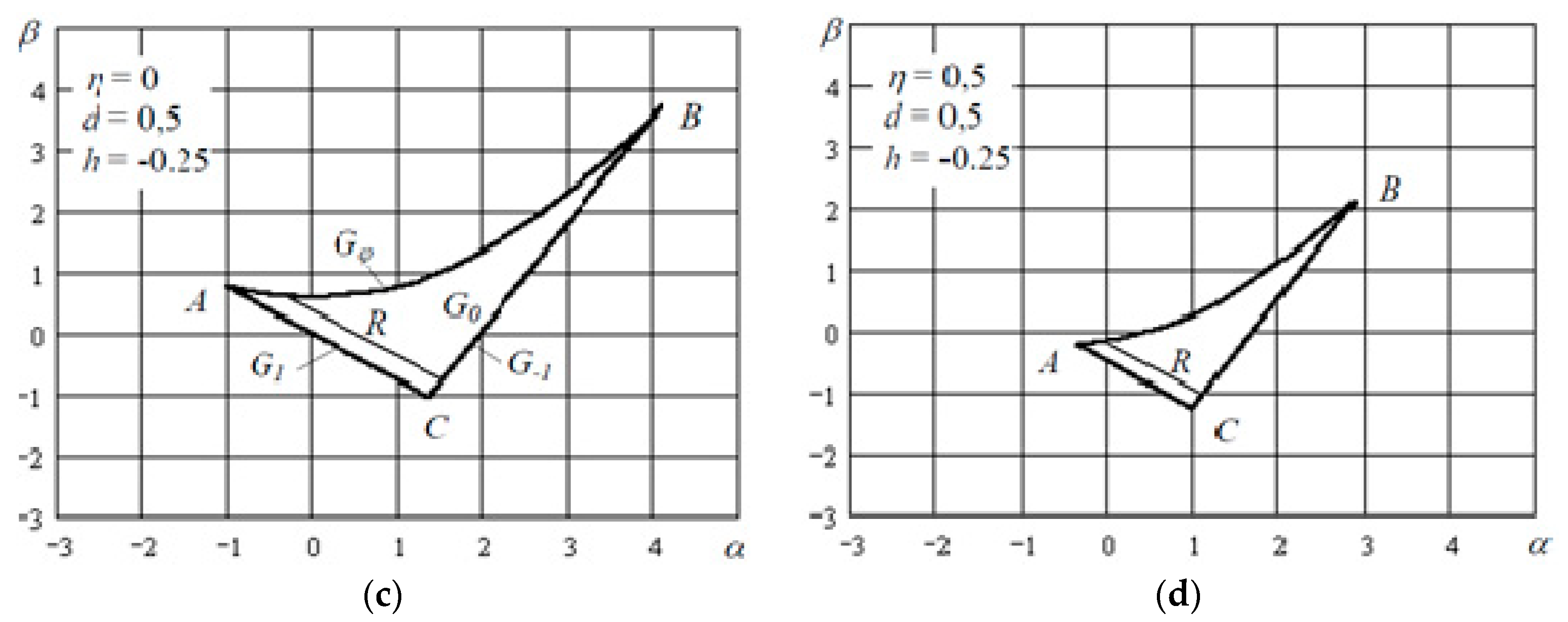
The cross sections of the local stability body of the mapping (Equation (1)) for various values of the generalized parameter n have a shape close to a triangular one. They are bounded by the curves G 1 , G 1 , G φ corresponding to the transition of one of the eigenvalues of the linearized matrix of the map (Equation (1)) through the values ± 1 or e ± j φ . The line R on the sections bounds the region of existence of a simple fixed point. Its equation is obtained from Equation (1) and it is written as follows:
β = g ( 1 d h ) α η .
The singularity of the transition of stability boundaries, in the case of a third order mapping, consists of a large variety of possible combinations of the eigenvalues of the linearized matrix A corresponding to the boundary.
In accordance with Table 1, when the boundary G 1 is crossed, there are also three types of nodes and with the transition of the vibrational boundary G φ , there are four types of foci. The transition through the boundaries G φ , G 1 occurs in the linear sections of the functions F 1 ( φ ) and F c ( φ ) . It is accompanied respectively by such bifurcations as a stable focus-complex saddle and a stable node, i.e. a real saddle. As in the case of second order mappings, the bifurcation data leads to the appearance of invariant closed curves, which are quasiperiodic motions. By virtue of the existence of a boundary R (for g 0 ) that does not coincide with G 1 for piecewise linear mappings, in the general case the bifurcations of the appearance of both simple and k-fold fixed points occur on this boundary. In this case, a fixed point (one of the types of a stable node or focus) is generated simultaneously with one of the types of a saddle fixed point. The disappearance of a fixed stable point also occurs at the boundary R because of the fusion of a stable node or focus with a saddle point, followed by the formation of a stream of densified trajectories. The condition for the appearance of a pair of fixed points on the boundaries of piecewise linear mappings will be laid down below as the basis for the method of calculating bifurcation parameters.
In Figure 1, sections of the local stability body of the mapping (Equation (1)) for various values of the generalized parameter n are given on the plane of generalized parameters a, b.
The formation of quasiperiodic motions under the conditions of the existence of fixed points is determined by the mutual arrangement of invariant separatrix manifolds of a simple or k-fold saddle fixed point. The difference from the second order mapping consists of a greater number of typical phase portraits near the saddle point, determined by the variety of the point itself.

3. SPS Model with Saw-Tooth Nonlinearity

The proposed method for calculating the bifurcation parameters of piecewise linear mappings of the third order is based on the assertions that fixed points on the boundaries of the linear sections of the functions F c ( φ ) and F 1 ( φ ) can arise. For the occurrence of simple fixed points of data, the assertions are sufficient. For the appearance of k-fold fixed points, the formulated assertions appear as necessary ones.
Let F ( φ ) = F 1 ( φ ) . Since F 1 ( φ ) is periodic, the phase space of the mapping (Equation (1)) is a three-dimensional cylinder, whose scan cross-sections are shown in Figure 2.
Figure 2 shows the section of the phase space by the plane y n = 0 . The lines L φ , 0 ( A B ) , L x , 0 ( C D ) and L y , 0 are sections of the surfaces of the map preserving the coordinates φ , x and y, respectively. The equations of these surfaces can be obtained from (Equation (1)) respectively with φ n + 1 = φ n , x n + 1 = x n , y n + 1 = y n :
L φ , 0 : x = α φ , L φ , 0 : x = ( y γ φ + g ) / ( 1 d ) , L φ , 0 : y = h x σ φ .
The mapping (display) surface with the preserved coordinate y is defined under the condition x n = x 01 . It should be noted that the coordinate y is not included in the equation for L φ , 0 , so the surface under consideration is perpendicular to the plane y = 0 . Moreover, the surface b passes through the origin of coordinates, and like in the second order system, it does not depend on the normalized initial detuning g. The point of intersection of these surfaces is the equilibrium state of the system (at the same time, the conditions φ n + 1 = φ n , x n + 1 = x n and y n + 1 = y n are satisfied, and has the coordinates O ( φ 01 , x 01 , y 01 ) .
By analogy with a system of the second order, domains of space can be found starting from which the solution (Equation (1)) falls on the boundary of the nonlinearity period F 1 ( φ ) φ n = 1 and φ n = 1 . The required domains are a set of planes G Q . m (the index m is the number of the period F 1 ( φ ) ) on whose boundary the solution falls) whose equations are written as follows [11,12,13,14,15,16,17]:
G Q . m : x = ( α 1 ) φ + 2 m 1 , m = 1 , 2 , 3
And
G Q . m : x = ( α 1 ) φ + 2 m + 1 , m = 1 , 2 , 3
In Equations (5) and (6), like in the expression for L φ , 0 , the coordinate y is not included, and consequently these planes are perpendicular to the plane y n = 0 .
The arrows show the directions of the motion of the state vector q n ( φ n , x n , y n ) along the directions φ n and x n under the mapping, in each of the four zones formed by the segments AB and CD. For some saddle points shown in Figure 2, quasiperiodic motions do not take place.
In Figure 2, the domains of the nonlinear mapping are shaded with output correspondingly to the boundaries φ n = + 1 and φ n = 1 of the phase cylinder scan Q 1 and Q 1 . On both sides, the domains Q 1 and Q 1 are bounded by the planes φ n = ± 1 , with the third one, by the plane x = 1 ( 1 α ) φ for Q 1 (mapping in the direction of increasing x n ) and the plane x = 1 ( 1 α ) φ for Q 1 (the mapping in the direction of decreasing φ n ). In the directions y n and one of the directions x n , the domains Q 1 and Q 1 are unbounded. Between the domains Q 1 and Q 1 there is a domain Q 0 , the map from which occurs linearly.
For a nonlinear mapping, the domain Q 1 passes to the domain Q 1 . Moreover, the point B ( 1 , α , 0 ) is mapped to the point B ( 1 ,    α d β + g ,    α h σ ) ; L ( 1 , 2 α , 0 ) to the point L ( 1 , d ( 2 α ) + β + g ,    h ( 2 α ) σ ) , and so on.
Changing the coordinate [ q n ] y of the state vector in the Q 1 , a domain leads to a change in the coordinate of the vector [ q n + 1 ] x in Q 1 : With increasing (decreasing) [ q n ] y increases (decreases) [ q n + 1 ] x . Thus, the entire domain Q 1 is mapped into an infinite strip along the x n -axis bounded along the φ n axis by the planes φ n = ± 1 and, in addition, by two parallel planes that are mappings of the planes φ n = ± 1 . Analogous arguments lead to the construction of the domain Q 1 , which is a mapping of Q 1 . It should be noted that there is an intersection of the domains Q 1 and Q 1 , as well as Q 1 and Q 1 , which fundamentally distinguishes the considered system from the second order system.
Let us consider iterations with initial conditions from an arbitrary state vector q 0 = ( φ 0 , x 0 , y 0 ) . According to (Equation (1)) vector q n may be expressed by means of q 0 as follows:
q n = A n q 0 + j = 0 n 1 A j ( r + p n j 1 )
where A is linearized matrix corresponding to (Equation (1)) under the linear mapping p j = ( 0 , 0 , 0 ) T , in the case of a nonlinear mapping p j = ( ± 2 , 0 , 0 ) T , with this, the sign "+" corresponds to going abroad φ = 1 , the sign "-" corresponds to going abroad x = + 1 . The vector p j returns the state vector of the system to the ( j + 1 ) -step in the interval [−1; 1] for the coordinate x. We rewrite (Equation (7)) as:
q n = A n q 0 + ( E A n ) ( E A ) 1 r + j = 0 n 1 A j p n j 1
For a cycle of period k existing, it is necessary that the closure condition q k = q 0 be satisfied. Taking this condition into account, the expression for the initial point of the cycle follows from (Equation (8)):
q n = ( E A k ) 1 ( j = 0 k 1 A j p k j 1 ) + ( E A ) 1 r
The expression (Equation (9)) may be considered as the first necessary condition for the existence of a cycle, or the closure condition. The second condition is to find all the state vectors of a cycle of a required structure within the interval | φ | 1 (i.e., the structural condition). Implementation of this condition means that all state vectors of the cycle are in the corresponding domains Q 1 , Q 0 , Q 1 . Otherwise, Equation (9) can formally lead to some state that is not a point of the cycle. The formulated conditions are necessary and sufficient for the existence of a cycle with a certain structure.
Similar to a discrete SPS of the second order, it can be shown that an arbitrary cycle existing in a system with nonlinearity F 1 ( φ ) is stable under the conditions of local stability of the mapping (Equation (1)).
Consider the structure cycle ( u / k ) , where u is the number of nonlinear mappings on the cycle period, k is the cycle period. For the limit cycle of the first kind u = 0 , for the limit cycle of the second kind in the case of rotation along the coordinate p in the direction of increasing u > 0 , in the case of rotation in the direction of decreasing the coordinate φ u < 0 . In accordance with (9), the vector of an arbitrary point of the cycle can be represented as follows:
q j = l j + g b , j = 1 , , k
where l j = ( E A k ) 1 ( j = 0 k 1 A j p k j 1 ) , b = ( E A ) 1 ( 0 , 1 , 0 ) T ; l j is a vector, depending on the structure of the cycle and the choice of the starting point, b is a vector depending neither on the structure of the cycle nor its initial state.
When g is changed, all points of the cycle in the phase domain are displaced along the vector b . This can lead to both the occurrence and destruction of the cycle due to the transition of cycle points between the domains Q 1 , Q 0 , Q 1 , and also when the points of the plane cycle φ n = ± 1 intersect the vectors.
Let us find conditions for the generalized detuning g for which there exists a cycle of a certain structure ( u / κ ) . To do this, we use the above conditions for the existence of a cycle. From (7–9) we assess the values of the generalized detuning g j and g + j for which the state vector q j intersects the boundaries φ n = 1 and φ n = + 1 , respectively:
g j = 1 [ l j ] 1 [ b j ] 1 , g + j = 1 [ l j ] 1 [ b j ] 1
All points of the cycle intersect the plane φ n = 1 if the condition g > max j = 1 k ( g j ) is satisfied, at least one cycle point intersects the plane φ n = 1 for g < min j = 1 k ( g j + ) . A cycle can exist when:
max j = 1 k ( g j ) < min j = 1 k ( g j + ) ,
in the detuning range max j = 1 k ( g j ) < g < min j = 1 k ( g j + ) .

4. Algorithm for Determining the Acquisition Bandwidth

We constructed an algorithm for determining the acquisition band. It is based on the condition of the occurrence of the simplest limit cycles of the first and second kind. In the general case, it is necessary to determine two values of the initial detuning γ min , γ max . With γ < γ max all PC2 disappear, with γ > γ min all PC1 disappear [16,17,18,19,20,21,22].
Let us find γ max , for this we define the value of γ k , at which the PC2 structures ( 1 / k ) appear. To be exact, we consider the initial state on the cycle to be the state into which the system comes after the nonlinear mapping through the boundary φ n = 1 . For this case p j = ( 0 , 0 , 0 ) T , 0   j   < k 1 ; p k 1 = ( 2 , 0 , 0 ) T . According to Equations (10)–(12), the initial state vector q 0 will be as follows [11,12,13,14,15,16,17]:
q 0 = P k 1 E A k + r E A
The cycle of the second kind of period k will exist when conditions (Equation (13)) are fulfilled and will occur, taking into account Equations (1) and (5) with frequency detuning
γ 2 k = 1 + 2 [ ( E A k ) 1 ] 11 ξ [ ( E A ) 1 ] 12
The boundary of the cycle generation may be expressed as follows:
γ = γ max = min k = 1 k max ( γ 2 k ) .
It remains to find k , for which the founded value of the initial detuning will be the smallest, which determines the boundary condition for the occurrence of PC2. The algorithm proposes the assignment of some k max , which obviously exceeds the desired value. Recommendations for choosing k max are similar to the second order system and are as follows. In the case of complex eigenvalues of the matrix A , the behavior of the vector l is oscillatory in parameter k (the end of the vector with an increase in the cycle period k describes a twisting spiral around a point ( 2 , 0 , 0 ) and it is enough to take half the oscillation period as k max .
The analysis of the above dependencies from the standpoint of global stability of the FAS leads to the following conclusions:
  • With increasing α 1 ,   α 2 , the stability domains with respect to the amplification D expand. The most significant increase is observed for large m 1 . For example, for m 1 = 0.8 with increasing α 1 ,   α 2 from values 0.5–0.8 (Figure 3) to values 2–4 (Figure 3), the stability domains in parameter D increase 2–4 times.
  • The boundary of the areas with global stability on the initial mismatch β also expands significantly with increasing α 1 ,   α 2 . However, dependence on m 1 is more complex. A decrease in the upper bound β with increasing m 1 is observed near the limits of the local stability. On the contrary, in the farther zone from the boundary of local stability (medium D ), there is a significant increase in the upper boundary β with increasing m 1 .
  • Limiting the stability of the bottom of the frequency detuning (limiting with the cycles of the first kind) is most expressed with small m 1 and, as stated above, is non-monotonous. The most significant restriction is observed for large D (Figure 3) and can reach values of 0.3–0.4.

5. SPS Model with a Triangular Nonlinearity

Let F ( φ ) = F c ( φ ) . The basic laws of the appearance of periodic motions of the second kind and quasiperiodic motions in a third order system with a triangular nonlinearity repeat at a qualitative level in the results obtained for a second order system [12,19,21,22,23,24,25]. In this case, both the final dependencies and the mechanisms explaining them are qualitatively repeated. In this regard, we will not dwell on them in detail below. The quantitative differences will be demonstrated on a number of graphs devoted to the analysis of the acquisition band.
The situation with cycles of the first kind, whose existence has been established in a system with a saw-tooth nonlinearity, is completely different. Their analysis is important because they have occurred with small initial detuning and limit the acquisition domain in frequency from below.
A quantitative estimate of the boundary of first kind cycles can be obtained by considering the change in the area of their existence in the parameter space with a change in the shape of the characteristic. Figure 5 shows the region of existence of PC1 on the plane D , γ for different values of c . The boundaries of the areas are almost straight lines, the slope of which depends only on the filter parameters ( α 1 ,   m 1 ,   α 2 ,   m 2 ). Changing c does not change the shape of these curves, but shifts them along the abscissa. PC1 cycles disappear in two cases: Firstly, at a certain maximum value of the parameter c max ; and secondly, with a saw-tooth characteristic of the detector and certain filter parameters (Figure 4).
The authors can note the strong influence of parameters on these dependencies.
From a practical point of view, the filter parameters are of a certain interest. Limit cycles of the first kind (quasi-synchronism mode) are impossible for them. Figure 5 shows the regions of existence of PC1 on the plane α 1 ,   α 2 with equal forcing coefficients m 1 ,   m 2 . For m 1 = m 2 = 0 , there is a boundary close to a straight line, above which there are no cycles. With increasing m 1 ,   m 2 , the area of existence of cycles is symmetrically limited by α 1 ,   α 2 , and disappears when m 1 =   m 2 0.165 .
Analysis of the above results shows that the existence of cycles of the first kind with a saw-tooth-like, or close to it, detector characteristic is determined only by the filter parameters and is not related to the gain of the system.
The dependencies in Figure 5 allow us to analyze the acquisition band when changing the duration of the stable branch of the detector characteristics and to answer the question about its optimal value. As in the case of pulsed DSC of the second order, for small D , a weak dependence of the acquisition band on the shape of the characteristics is observed. There is some loss for F c ( φ ) , increasing with the steepness of the stable branch.
With increasing D (to the boundary of local stability) due to a shift in the boundary of the onset of quasiperiodic motions towards large β , the maximum of the acquisition band is provided in the case of F c ( φ ) . With different ratios of filter parameters, the gain in the acquisition band can reach up to 50% as compared with F c ( φ ) . Figure 5 also shows the limitations of the acquisition area from below due to PC1. It is possible to get rid of such restrictions by increasing the steepness (decreasing the duration) of a stable part of the characteristics.

6. Results

The dual-ring synthesizer was simulated. The computer model made it possible to take into account a number of factors additionally, which were not considered in the mathematical model. They included the inconstancy of the discretization periods and the difference between the detector model and the zero order extrapolator.
Allowance for variations of the sampling period (epoch) resulted in corrections of the dynamic characteristics, primarily the stability domain. However, this applied mainly to the range of large gains (α > 1, β > 1). For operating gains, the results of mathematical and computer simulation coincided with high accuracy [25,26,27,28].
Figure 6 shows the dependences of the capture band and the transient time of the dual-ring SPS, taking into account the variable nature of the sampling periods, for k1 / k2 = 8. To compare, Figure 6a shows the results for a constant sampling period (upper curves). With positive detuning, allowance for the variations led to a certain decrease in the capture band, repeating the known result for single-ring systems. A change in the capture band as a function of μ repeated similar changes for a model with a constant sampling period. A decrease in the capture band with increasing μ was observed. Changing the sign of μ to the opposite, resulted in an increase in the capture band, partially offsetting the loss from the variations in the sampling period.
An analysis of the average time for the frequency settling in a dual-ring SPS (Figure 6b–d) suggested a qualitative coincidence with the results of the model analysis [6,8].
In particular, there is was a fairly wide range of parameters (shown in the Figure for gains), where the frequency setting time was rather small and almost invariable. It confirmed the stabilizing effect of mutual bonds (the results are given to establish the frequency with an accuracy of 0.01 F). A certain range shift to the left was explained by an increase in the equivalent gain due to the variable sampling period. According to the above results, for filter parameters that provided suppression at a sampling frequency close to 10 dB (m = 0.5, αΦ = 0.5–1.0), the time for setting the frequency did not exceed 10 samples of the output ring in a wide range of gains.

7. Conclusions

Based on the general provisions of the theory of bifurcations, the directions for analyzing the conditions for the occurrence of periodic and quasiperiodic motions in a third order DCS with a piecewise linear characteristic of the detector are defined. As in the case of the second order DCS, the basis for the occurrence and loss of stability of k-multiple fixed points is the condition that the linear sections fall on the boundaries of linear sections. The mandatory requirement for the occurrence of quasiperiodic motions is the contact of the incoming and outgoing separatrix manifolds by a saddle point. The difference from the second order systems is in a large number of different types of saddle points and, accordingly, the number of possible scenarios of motions in the neighborhood of separatrix manifolds.
The method of estimating the bifurcation parameters of piecewise linear mappings of the third order has been developed. This makes it possible to find the boundaries of areas of the existence of various types of periodic and quasiperiodic motions. The method is based on the mandatory and sufficient conditions for the occurrence of a k-multiple fixed point through the formation of an intermediate complex point node-saddle or focus-saddle and the conditions for tangency of the incoming and outgoing separatrix manifolds at the boundaries of the linear sections of the characteristics.

Author Contributions

S.S. investigated the mathematical structure of the model; A.Z. described mathematical models and their formalization; S.C. carried out the analysis of mathematical structures and components and analysis of references; A.N. described and analyzed the analysis of mathematical components of algorithmization; D.M. investigated graphic structures and components.

Funding

This research was funded by Admiral Makarov State University of Maritime and Inland Shipping.

Conflicts of Interest

The authors declare no conflict of interest.

References

  1. Li, S.; Chen, G.; Mou, X. On the Dynamical Degradation of Digital Piecewise Linear Chaotic Maps. Int. J. Bifurc. Chaos 2005, 15, 3119–3151. [Google Scholar] [CrossRef]
  2. Nie, X.; Coca, D. A matrix-based approach to solving the inverse Frobenius–Perron problem using sequences of density functions of stochastically perturb e d dynamical systems. Commun. Nonlinear Sci. Numer. Simulat. 2018, 54, 248–266. [Google Scholar] [CrossRef] [PubMed]
  3. Guariglia, E. Harmonic symmetry of the Riemann zeta fractional derivative. AIP Conf. Proc. 2018, 2046, 020035. [Google Scholar]
  4. Guido, R.C.; Addison, P.; Walker, J. Introducing wavelets and time-frequency analysis. IEEE Eng. Biol. Med. Mag. 2009, 28, 13. [Google Scholar] [CrossRef] [PubMed]
  5. Guido, R.C. Effectively interpretating discrete wavelet transforms signals. IEEE Signal Process. Mag. 2017, 34, 89–100. [Google Scholar] [CrossRef]
  6. Gutkin, L.S. Designing Radio Systems and Radio Devices: Proc. Manual for Universities. Radio and Communication. 1986. Available online: https://www.rsl.ru/Gutkin/14579_ls (accessed on 10 April 2018).
  7. Shahgildyan, V.V. Radio Transmitting Devices. Radio and Communication. 1990. Available online: https:// publ.lib.ru/ARCHIVES/SH/SHAHGIL’DYAN_Vagan (accessed on 15 April 2018).
  8. Akimov, V.N. Phase-synchronization Systems. Radio and Communication. 1982. Available online: https://www.rsl.ru/127 (accessed on 11 May 2018).
  9. Best, R.E. Phase-Locked Loops: Design, Simulation, and Application, 3rd ed.; McGrow-Hill: New York, NY, USA, 1997; 360p. [Google Scholar]
  10. Kazakov, L.N.; Paley, D.E.; Ponomarev, N.Y. Comparative Analysis of the Nonlinear Dynamics of Discrete Autonomous SPS of the 2nd and 3rd Orders. 1999. Available online: https: //www.elar.uniyar.ac.ru/jspui/bitstream/19/kln_5 (accessed on 20 January 2017).
  11. Kazakov, L.N.; Paley, D.E. Analysis of the Capture Band of a Third-order Pulse Phase-locking System with a Sawtooth Characteristic of the Detector. Radiotekhnika. 1998. Available online: https: //www.elar.uniyar.ac.ru/jspui/bitstream/129/1/kln_1_a (accessed on 10 March 2017).
  12. Fomin, A.F.; Khoroshavin, A.I.; Shelukhin, O.I. Analog and Digital Synchronous-phase Meters and Demodulators. Radio and communication. 1987. Available online: https://www.bsuir.by/m/12_119786_1_86932 (accessed on 30 April 2018).
  13. Manchur, G.; Erven, C. Development of a Mode1 for Predicting Flicker from Electric Are Fumaces. IEEE Trans. Power Deliv. 1992, 7, 416–426. [Google Scholar] [CrossRef]
  14. Zhilenkov, A.; Chernyi, S. Investigation performance of marine equipment with specialized information technology. Procedia Eng. 2015, 100, 1247–1252. [Google Scholar] [CrossRef]
  15. Zhilenkov, A.; Chernyi, S. Models and Algorithms of the Positioning and Trajectory Stabilization System with Elements of Structural Analysis for Robotic Applications. Int. J. Embed. Syst. 2019, in press. [Google Scholar]
  16. Chernyi, S.; Zhilenkov, A. Modeling of complex structures for the ship’s power complex using XILINX system. Transp. Telecommun. 2015, 16, 73–82. [Google Scholar] [CrossRef]
  17. IEEE Working Group on Power System Harmonic. Bibliography of Power System Harmonics, Part 1 and Ii. Papers 84WM 214-3. In Proceedings of the IEEE PES Winter Meeting, Dallas, TX, USA, 29 January–3 February 1984. [Google Scholar]
  18. IEEE Working Group on Power System Harmonic. Power System Harmonics: An Overview. IEEE Trans. Power Appar. Syst. 1983, PAS-102, 2455–2460. [Google Scholar] [CrossRef]
  19. Singh, B.; Al-Haddad, K.; Chandra, A. A Review of Active Filters for Power Quality Improvements. IEEE Trans. Ind. Electron. 1999, 46, 960–971. [Google Scholar] [CrossRef]
  20. Govindarajan, S.N. Survey of Harmonic Levels on the Southwestern Electric power Company System. IEEE Trans. Power Deliv. 1991, 6, 1869–1873. [Google Scholar] [CrossRef]
  21. Ding, Q.; Yang, Z.H. Secure Communication System Based on Hardware Logic Encryption; Posts & Telecom Press: Beijing, China, 2015. [Google Scholar]
  22. Sokolov, S.; Zhilenkov, A.; Chernyi, S.; Nyrkov, A. Assessment of the Impact of Destabilizing Factors in the Main Engine Shaft of the Adaptive Speed Controller. Procedia Comput. Sci. 2018, 125, 420–426. [Google Scholar] [CrossRef]
  23. Malioutov, D.; Corum, A.; Cetin, M. Covariance Matrix Estimation for Interest-Rate Risk Modeling via Smooth and Monotone Regularization. IEEE J. Sel. Top. Signal Process. 2016, 10, 1006–1014. [Google Scholar] [CrossRef]
  24. Chaudhuri, A.; Stenger, H. Survey Sampling Theory and Methods. 2005. Available online: https://www.rsl.ru/ (accessed on 2 March 2018).
  25. Nyrkov, A.; Zhilenkov, A.; Sokolov, S.; Chernyi, S. Hard- and Software Implementation of Emergency Prevention System for Maritime Transport. Autom. Remote Control 2018, 79, 195–202. [Google Scholar] [CrossRef]
  26. Alekseev, G.D.; Karpovich, V.A. Power installations of fishing vessels. Shipbuilding. 1972. Available online: https://www.taylorfrancis.com/books/9781420028638 (accessed on 5 May 2017).
  27. Sokolov, S.; Zhilenkov, A.; Nyrkov, A.; Chernyi, S. The Use Robotics for Underwater Research Complex Objects. Adv. Intell. Syst. Comput. 2017, 556, 421–427. [Google Scholar]
  28. Chernyi, S.; Zhilenkov, A.; Sokolov, S.; Nyrkov, A. Algorithmic approach of destabilizing factors of improving the technical systems efficiency. Vibroengineering PROCEDIA 2017, 13, 261–265. [Google Scholar] [CrossRef] [Green Version]
Figure 1. Cross-sections of the body with the local stability synchronization systems of the third order ((a) η = 1.2 ; (b) η = 0.6 ; (c) η = 0 ; (d) η = 0.5 ).
Symmetry 11 00236 g001aSymmetry 11 00236 g001b
Figure 2. Phase cylinder cross section.
Symmetry 11 00236 g002
Figure 3. Acquisition band SFS of the third ((a) α 1 = 0.5 ; (b) α 1 = 1 ) order with F 1 ( φ ) .
Symmetry 11 00236 g003
Figure 4. Shows the dependences of c max on the time constant of one of the links of the filter.
Symmetry 11 00236 g004
Figure 5. The acquisition band of the pulsed SPS ((a) α 1 = 1 ; (b) α 1 = 10 ) with F c ( φ ) .
Symmetry 11 00236 g005
Figure 6. Dependencies of the capture band and the settling time in the dual-ring SPS ((a) μ = 0.1 ; (b) μ = 0.1 ; (c) m 1 = 0 ; (d) m 1 = 0.5 ).
Symmetry 11 00236 g006
Table 1. Parameters for solving.
The Eigenvalues of the Matrix AType of a Stable Point
1) 0 < p < 1, 0 < p2 < 1, 0 < p3 < 1, p1, p2, p3 are real-valuedstable node of the 1st type
2) −1 < p3 < 0, p1, p2, p3 are real-valued.stable node of the 2nd type
3) 0 < p < 1, are real-valuedstable node of the 3rd type
4) 0 < p < 1, 0 < p2 < 1, −1 < pb < 0, pl, p2, p3 are real-valuedstable node of the 4th type
5) 0 < Re < l are real-valued, p2, p3stable focus of the 1st type
6) −l < Re < 0stable focus of the 2nd type
7) 0 < R < l; px are real-valued, p2, p3stable focus of the 3rd type
8) −1 < p < 0, are real-valued, p2, p3 stable focus of the 4th type

