A Novel Computational Technique for Impulsive Fractional Differential Equations

Abstract

A computational technique for impulsive fractional differential equations is proposed in this paper. Adomian decomposition method plays an efficient role for approximate analytical solutions for ordinary or fractional calculus. Semi-analytical method is proposed by use of the Adomian polynomials. The method successively updates the initial values and gives the numerical solutions on different impulsive intervals. As one of the numerical examples, an impulsive fractional logistic differential equation is given to illustrate the method.

1. Introduction

Fractional calculus appears frequently in various applied topics [1,2,3,4,5,6,7] and pure mathematics [8,9,10,11,12]. They are employed to depict the long-interaction of different statues of the systems. The fractional order controls the amount of dependence on past information and shows the quantity of the memory. On the other hand, as a result, it holds both quantitative and qualitative aspects. It shows some features that are not present in other tools. This is the main reason for the popularity of the fractional calculus as a modeling tool for the memory process.

Impulse theory is often used in control methods of differential equations. The impulsive point changes dynamics of continuous time systems locally. Then, the solution has a jump and becomes a piecewise continuous function on the whole interval, and impulsive points are the endpoints of each short interval. A differential equation containing impulses is also called a system with a jump. Hence, the impulsive differential equation is not a continuous time system but the one combining both continuous and discrete point information. It depicts the impact of external conditions which may be negative or positive. Impulsive fractional differential equations have received much attention recently [13,14,15,16,17,18,19]. It can illustrate totally distinct dynamics in comparison to standard fractional systems, and this property has often been adopted in fractional impulsive control. Many analytical methods have been efficiently developed for differential equations [20,21,22,23,24,25,26,27]. However, the less numerical method and analytical method were developed for impulsive fractional differential equations. In this study, our main purpose is to extend methods from the integer order to the fractional order.

The Adomian decomposition method (ADM) has been applied in various nonlinear problems, and the Adomian polynomials play a crucial role in the treatment of the nonlinear terms in fractional differential equations. Recently, Duan et al. proposed a new way to calculate the polynomials which can derive the same results but greatly improve computational speed and save time in comparison with the classical one. Hence, various novel algorithms based on the new Adomian polynomials can be considered now. It was successfully used in fractional differential equations [28] where a semi-analytical method was developed.

In this paper, a novel computational technique is proposed for the following equation by use of new Adomian polynomials [21,22,23]:

$$\{\begin{array}{l}{}_{t_0}{}^{\mathrm{C}}D_t^{\alpha }x(t)=F(t,x),t\in J\prime :=J\backslash \left[t_{N_1},\cdots ,t_{N_M}\right],J:=\left[t_0,T\right],\\ \Delta x_{N_k}=I_k\left(x_{N_k}^{-}\right)=x\left(t_{N_k}^{+}\right)-x\left(t_{N_k}^{-}\right)=y_k,1\le k\le M,\\ x_k=x(t_k),x\left(t_{N_k}^{+}\right)=\underset{\hslash \to \infty }{\lim }x\left(t_{N_k}+\hslash \right),x\left(t_k^{-}\right)=\underset{\hslash \to 0}{\lim }x\left(t_{N_k}-\hslash \right),\\ \hslash >0,x(t_0)=x_0.\end{array}$$

(1)

The Adomian polynomials are used in fractional differential equations. However, to the best of our knowledge, we did not find any work on semi-analytical solutions for impulsive fractional differential equations. This paper combines both analytical and numerical solutions’ features to develop a semi-analytical method.

2. Preliminaries

2.1. Definitions and Properties of Fractional Calculus

The fractional calculus is defined as the following:

Definition 1

[1]. The Riemann–Liouville (R-L) integral of $\mathsf{\alpha }$ order is defined by

$${}_{t_0}{I}_t^{\alpha }f(t)=\frac{1}{\mathsf{\Gamma }(\alpha )}{\displaystyle {\int }_{\hspace{0.17em}{t}_0}^{\hspace{0.17em}t}}{(t-\mathsf{\tau })}^{\alpha -1}f(\mathsf{\tau })\hspace{0.17em}d\mathsf{\tau },\hspace{0.17em}0<t,0<\mathsf{\alpha }.$$

(2)

Definition 2

[1]. The R–L derivative is defined as

$$\begin{array}{l}{}_{t_0}D_t^{\alpha }f=\frac{1}{\mathsf{\Gamma }(m-\alpha )}\frac{d^m}{d{t}^m}{\displaystyle {\int }_{\hspace{0.17em}{t}_0}^{\hspace{0.17em}t}}\frac{1}{{(t-\mathsf{\tau })}^{\alpha -m+1}}f(\mathsf{\tau })\hspace{0.17em}d\mathsf{\tau },\hspace{0.17em}\\ \hspace{0.17em}{t}_0<t,0<\mathsf{\alpha },\hspace{0.17em}m=[\mathsf{\alpha }]+1,\end{array}$$

(3)

where Γ is the Gamma function.

Definition 3

[1]. The Caputo derivative is defined as

$$\begin{array}{l}{}_{t_0}{}^{C}D_t^{\alpha }f={}_{t_0}D_t^{\alpha }(f(t)-{\displaystyle \sum _{k=0}^{m-1}\frac{{(t-t_0)}^k}{k!}}{f}^{(k)}(t_0)),\hspace{0.17em}\\ \hspace{0.17em}0<t,0<\mathsf{\alpha },\hspace{0.17em}m=[\mathsf{\alpha }]+1.\end{array}$$

(4)

Remarks:

For Definition 3, the Caputo derivative of a constant is zero;

If $f(t)\in C^m([t_0,\infty ),R)$, then the Caputo derivative can be rewritten as

$${}_{t_0}{}^{C}D_t^{\alpha }f=\frac{1}{\mathsf{\Gamma }(m-\alpha )}{\displaystyle {\int }_{\hspace{0.17em}{t}_0}^{\hspace{0.17em}t}}\frac{1}{{(t-\mathsf{\tau })}^{\alpha -m+1}}\frac{d^m}{d{\mathsf{\tau }}^m}f(\mathsf{\tau })\hspace{0.17em}d\mathsf{\tau }.$$

(5)

In Definition 3, the function $f(t)$ can be discrete if it is integrable such that the fractional impulsive equation makes sense at the impulsive point.

In the sequel, we all use the definition of the Caputo derivative. We need the integral transform so that the fractional differential equation can be reduced to an integral one and the integral methods can be applied straightforward.

Property 1.

The Leibniz integral law holds

$$\begin{array}{l}{}_{t_0}{I}_t^{\alpha }{}_{t_0}{}^{C}D_t^{\alpha }f(t)=f(t)-f(t_0),\\ \hspace{0.17em}{t}_0\le t,0<\mathsf{\alpha }\le 1.\end{array}$$

(6)

Lemma 1

[14].The impulsive fractional differential Equation (1) is equivalent to the following integral equation of fractional order

$$\{\begin{array}{c}x(t)=x_0+{}_{t_0}I_t^{\alpha }F(t,x),\hspace{0.17em}t\in [t_0,t_{N_1}],\hfill \\ x(t)=x_0+y_1+{}_{t_0}I_t^{\alpha }F(t,x),\hspace{0.17em}t\in (t_{N_1},t_{N_2}],\hfill \\ x(t)=x_0+y_1+y_2+{}_{t_0}I_t^{\alpha }F(t,x),\hspace{0.17em}t\in (t_{N_2},t_{N_3}],\hfill \\ ⋮\\ x(t)=x_0+{\displaystyle \sum _{j=1}^k{y}_j}+{}_{t_0}I_t^{\alpha }F(t,x),\hspace{0.17em}\hspace{0.17em}t\in (t_{N_k},t_{N_{k+1}}],\hfill \\ ⋮\\ x(t)=x_0+{\displaystyle \sum _{j=1}^M{y}_j}+{}_{t_0}I_t^{\alpha }F(t,x),\hspace{0.17em}t\in (t_{N_M},T],\hspace{0.17em}1<N_M.\hfill \end{array}$$

(7)

2.2. Adomian Polynomials

Considering a nonlinear equation

$$x(t)=G(x(t))$$

(8)

for the nonlinear term $G(x(t))$, the Adomian polynomial named after G. Adomian [29] can be obtained by

$$A_n=\frac{1}{n!}\frac{{\partial }^n}{\partial {\lambda }^n}(G[{\displaystyle \sum _{k=0}^{\infty }{x}_k{\lambda }^k}]){|}_{\lambda =0}.$$

(9)

With the known values of $x_0,\cdots ,x_n$, we can successively obtain $A_n$.

Duan [21,22,23] newly proposed a fast Adomian polynomial as the following

$$A_n=\frac{1}{n}{\displaystyle \sum _{k=0}^{n-1}(k+1)x_{k+1}\frac{\partial A_{n-1-k}}{\partial x_0}},A_0=G(x_0)$$

(10)

Generally, the one of the z-variable is calculated by

$$A_n=\frac{1}{n}{\displaystyle \sum _{i=1}^z{\displaystyle \sum _{k=0}^{n-1}(k+1)x_{i,k+1}\frac{\partial A_{n-1-k}}{\partial x_{i,0}}}},i=1,\dots ,z.$$

(11)

Although both lead to the same analytical solution, the new one is given in a more concise form and saves computational time. This is very important for solutions of the fractional calculus since the fractional derivative has the memory effects and can possess a large storage space.

3. Semi-Analytical Method Based on Adomian Polynomials

Consider the following fractional system with impulse (1). Using the idea by Duan [21], we give steps of a novel algorithm for impulsive fractional differential equations.

• Assume the solution in a series form as

  $$x(t)={\displaystyle \sum _{i=0}^{\infty }{c}_i{(t-t_0)}^{i\mathsf{\alpha }}}$$

  (12)

  and $x_n$ is assumed as ${\displaystyle \sum _{i=0}^n{c}_i{(t-t_0)}^{i\mathsf{\alpha }}}$ accordingly.
• Substituting (12) into (8), with Adomian polynomials, the coefficients of $c_i$ are obtained as

  $$\{\begin{array}{l}{c}_{n+1}=\frac{\mathsf{\Gamma }(1+n\mathsf{\alpha })}{\mathsf{\Gamma }(1+(n+1)\mathsf{\alpha })}{A}_n[c_0,c_1,\dots ,c_n],0\le n,\\ c_0=x_0+{\displaystyle \sum _{j=1}^k{y}_{ j}}.\end{array}$$

  (13)
• $x_n$ can be obtained as

  $$x_n=\psi (c_0,t_0,{\displaystyle \sum _{j=1}^k{y}_{ j},t}),t\in (t_{N_k},t_{N_{k+1}}].$$

  (14)
• Set $t\in [t_0,T]$, $t=ih$, $H=\frac{T}{N}$, $h=\frac{H}{K}$, $i=0,1,\dots ,NK$ and let $x_i^{*}=\psi (x_{i-1}^{*},t_{i-1},{\displaystyle \sum _{j=1}^k{y}_j,\hspace{0.17em}}{t}_i),$ where $x_0^{*}=c_0$. We can obtain the numerical solutions $x_0^{*},\dots ,x_i^{*}$.

4. Numerical Solutions based on Adomian Polynomials

In this section, we consider an application of the method to Caputo fractional differential equations with impulses

$$\{\begin{array}{l}{}_{t_0}{}^{C}D_t^{\alpha }x(t)=\mu x(t)(1-x(t)),\\ t\in J\prime :=J\backslash [t_{N_1},\dots ,t_{N_M}],J:=[t_0,T]\\ \Delta x_k=y_k,x_k=x(t_k),y_k=0.1\\ x(t_0)=x_0=0.2,t_0=0.\end{array}$$

(15)

By use of Lemma 1, we have an integral equation as

$$\{\begin{array}{c}x(t)=x_0+{\mu }_{t_0}{I}_t^{\alpha }x(t)(1-x(t)),\hspace{0.17em}\hspace{0.17em}t\in [t_0,t_{N_1}],\hfill \\ x(t)=x_0+y_1+{\mu }_{t_0}{I}_t^{\alpha }x(t)(1-x(t)),\hspace{0.17em}\hspace{0.17em}t\in (t_{N_1},t_{N_2}],\hfill \\ x(t)=x_0+y_1+y_2+{\mu }_{t_0}{I}_t^{\alpha }x(t)(1-x(t)),\hspace{0.17em}\hspace{0.17em}t\in (t_{N_2},t_{N_3}],\hfill \\ ⋮\\ x(t)=x_0+{\displaystyle \sum _{j=1}^k{y}_j}+{\mu }_{t_0}{I}_t^{\alpha }x(t)(1-x(t)),\hspace{0.17em}t\in (t_{N_k},t_{N_{k+1}}],\hfill \\ ⋮\\ x(t)=x_0+{\displaystyle \sum _{j=1}^M{y}_j}+{\mu }_{t_0}{I}_t^{\alpha }x(t)(1-x(t)),\hspace{0.17em}\hspace{0.17em}t\in (t_{N_M},T],\hspace{0.17em}1<N_M.\hfill \end{array}$$

(16)

Adopt the semi-analytical method in Section 3. We have the recurrence relationship of the coefficients as

$$\{\begin{array}{l}{c}_{n+1}=\frac{\mathsf{\Gamma }(1+n\mathsf{\alpha })}{\mathsf{\Gamma }(1+(n+1)\mathsf{\alpha })}{A}_n[c_0,c_1,\dots ,c_n],0\le n,\\ c_0=x_0+{\displaystyle \sum _{j=1}^k{y}_k},1\le k\le M.\end{array}$$

(17)

We give the first few coefficients here

$$\{\begin{array}{l}{c}_1=\frac{\mathsf{\Gamma }(1)}{\mathsf{\Gamma }(1+\mathsf{\alpha })}(\mu c_0-\mu c_0^2),\\ c_2=\frac{\mathsf{\Gamma }(1+\mathsf{\alpha })}{\mathsf{\Gamma }(1+2\mathsf{\alpha })}({\mu }^2{c}_0-3{\mu }^2{c}_0^2+2{\mu }^2{c}_0^3),\\ c_3=\frac{\mathsf{\Gamma }(1+2\mathsf{\alpha })}{\mathsf{\Gamma }(1+3\mathsf{\alpha })}(-6{\mu }^3{c}_0^2+10{\mu }^3{c}_0^3-5{\mu }^3{c}_0^4+{\mu }^3{c}_0^{}),\\ \hspace{0.17em}\hspace{0.17em}\hspace{0.17em}\hspace{0.17em}\hspace{0.17em}\hspace{0.17em}\hspace{0.17em}\hspace{0.17em}\hspace{0.17em}\hspace{0.17em}\hspace{0.17em}\hspace{0.17em}\hspace{0.17em}\hspace{0.17em}\hspace{0.17em}\hspace{0.17em}\hspace{0.17em}\hspace{0.17em}\hspace{0.17em}\hspace{0.17em}\hspace{0.17em}⋮\end{array}$$

(18)

such that we determine the approximate analytical expression of series solutions.

We vary the parameters $\mathsf{\alpha }$ and $M$ to observe the behavior. In Figure 1, the fractional order $\mathsf{\alpha }=0.9$ and the number of impulsive points is set to 5. We can see that, with the increase in $M$ (See Figure 2 and Figure 3), the solutions’ values also increase if all of the impulse is positive. Figure 4 illustrates the stable solution without an impulse in the same fractional case. From all of the figures, we can observe that our semi-analytical solutions are plotted on the interval [0,10] which holds a longer time domain than the standard one.

Figure 1. Numerical simulation:$\mathsf{\alpha }=0.9,M=5$.

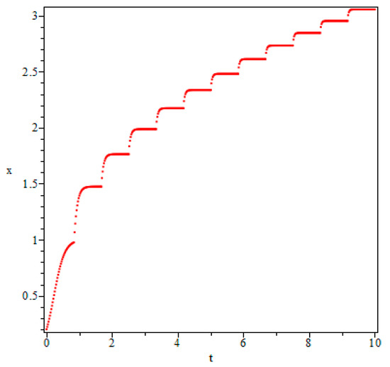
Figure 2. Numerical simulation:$\mathsf{\alpha }=0.9,M=11$.

Figure 3. Numerical simulation:$\mathsf{\alpha }=0.9,M=19$.

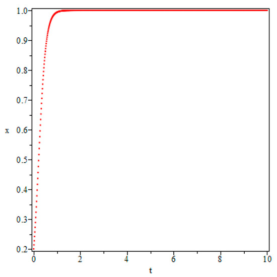
Figure 4. Numerical simulation: $\mathsf{\alpha }=0.9,$ without impulse.

5. Conclusions

Impulsive fractional differential equation has recently become an important topic, but less work has focused on numerical or analytical methods. In this paper, we develop an efficient method for nonlinear equations. New Adomian polynomials are adopted to treat the nonlinear terms, and a semi-analytical method is developed. Firstly, the impulsive fractional differential equation is given equivalently in an integral equation. Fractional Taylor series is implemented to derive a recurrence relationship. Since there is no differential or integral calculus, it becomes very quick and saves computational time to derive the analytical or numerical solutions in comparison with classical ADM. The semi-analytical solution shows that the method is very efficient. However, there are still some difficulties that we need to overcome in future. The following topics are also disadvantages that we will try to address:

• It is still challenging work to do error analysis. For many nonlinear cases, the exact solution is unknown and numerical errors cannot be obtained. We will pay attention to this topic in the near future;
• In this method, we generally adopt a fractional series expansion which is a fractional analogy of the Taylor series. What about other expansions which satisfy the features of the new polynomials? For example, how can series solutions be found for boundary value problems? Hence, it is very important to develop new ideas for this topic.

References

- Kilbas, A.A.; Srivastava, H.M.; Trujillo, J.J. Theory and Applications of the Fractional Differential Equations; North-Holland Mathematics Studies; Elsevier Science Limited: New York, NY, USA, 2006. [Google Scholar]
- Diethelm, K. The Analysis of Fractional Differential Equations; Springer: New York, NY, USA, 2010. [Google Scholar]
- Machado, J.T.; Kiryakova, V.; Mainardi, F. Recent history of fractional calculus. Commun. Nonlinear Sci. Numer. Simul. 2011, 16, 1140–1153. [Google Scholar] [CrossRef]
- Agarwal, R.; Hristova, S.; O’Regan, D. A survey of Lyapunov functions, stability and impulsive Caputo fractional differential equations. Fract. Calc. Appl. Anal. 2016, 19, 290–318. [Google Scholar] [CrossRef]
- Baleanu, D.; Diethelm, K.; Scalas, E.; Trujillo, J.J. Fractional Calculus: Models and Numerical Methods; World Scientific: Singapore, 2012. [Google Scholar]
- Mohammadi, F.; Cattani, C. A generalized fractional-order Legendre wavelet Tau method for solving fractional differential equations. J. Comput. Appl. Math. 2018, 339, 306–316. [Google Scholar] [CrossRef]
- Cattani, C. Sinc-Fractional Operator on Shannon Wavelet Space. Front. Phys. 2018, 6, 118. [Google Scholar] [CrossRef]
- Li, C.; Dao, X.; Guo, P. Fractional derivatives in complex planes. Nonlinear Anal. 2009, 71, 1857–1869. [Google Scholar] [CrossRef]
- Guariglia, E. Fractional Derivative of the Riemann Zeta Function. In Fractional Dynamics; Cattani, C., Srivastava, H.M., Yang, X.J., Eds.; De GruyterOpen: Warsaw/Berlin, Germany, 2015; pp. 357–368. [Google Scholar]
- Atangana, A.; Baleanu, D. New Fractional Derivatives with Nonlocal and Non-Singular Kernel: Theory and Application to Heat Transfer Model. Thermal Sci. 2016, 20, 1–7. [Google Scholar] [CrossRef]
- Guariglia, E.; Silvestrov, S. A functional equation for the Riemann zeta fractional derivative. AIP Conf. Proc. 2017, 1798, 020063. [Google Scholar]
- Ortigueira, M.D.; Rodríguez-Germá, L.; Trujillo, J.J. Complex Grünwald-Letnikov, Liouville, Riemann-Liouville, and Caputo derivatives for analytic functions. Commun. Nonlinear Sci. Numer. Simul. 2011, 16, 4174–4182. [Google Scholar] [CrossRef]
- Mophou, G.M. Existence and uniqueness of mild solutions to impulsive fractional differential equations. Nonlinear Anal. TMA 2010, 72, 1604–1615. [Google Scholar] [CrossRef]
- Feckan, M.; Zhou, Y.; Wang, J. On the concept and existence of solution for impulsive fractional differential equations. Commun. Nonlinear Sci. Numer. Simul. 2012, 17, 3050–3060. [Google Scholar] [CrossRef]
- Stamova, I.; Stamov, G. Stability analysis of impulsive functional systems of fractional order. Commun. Nonlinear Sci. Numer. Simul. 2014, 19, 702–709. [Google Scholar] [CrossRef]
- Wang, J.R.; Feckan, M.; Zhou, Y. On the new concept of solutions and existence results for impulsive fractional evolution equations. Dyn. Part. Differ. Equ. 2011, 8, 345–361. [Google Scholar]
- Wang, J.R.; Zhou, Y.; Feckan, M. Nonlinear impulsive problems for fractional differential equations and Ulam stability. Comput. Math. Appl. 2012, 64, 3389–3405. [Google Scholar] [CrossRef]
- Zhang, X.M. On the concept of general solution for impulsive differential equations of fractional-order q is an element of (1,2). Appl. Math. Comput. 2015, 268, 103–120. [Google Scholar]
- Zhang, X.M. On impulsive partial differential equations with Caputo-Hadamard fractional derivatives. Adv. Differ. Equ. 2016, 2016, 281. [Google Scholar] [CrossRef]
- He, J.H. Approximate analytical solution for seepage flow with fractional derivatives in porous media, Comput. Method. Appl. Mech. Eng. 1998, 167, 57–68. [Google Scholar] [CrossRef]
- Duan, J.S. An efficient algorithm for the multivariable Adomian polynomials. Appl. Math. Comput. 2010, 217, 2456–2467. [Google Scholar] [CrossRef]
- Duan, J.S. Recurrence triangle for Adomian polynomials. Appl. Math. Comput. 2010, 216, 1235–1241. [Google Scholar] [CrossRef]
- Duan, J.S. Convenient analytic recurrence algorithms for the Adomian polynomials. Appl. Math. Comput. 2011, 217, 6337–6348. [Google Scholar] [CrossRef]
- He, W. Adomian decomposition method for fractional differential equations of Caputo-Hadamard type. J. Comput. Complex. Appl. 2016, 2, 160–162. [Google Scholar]
- Wu, G.C.; Baleanu, D.; Deng, Z.G. Variational iteration method as a kernel constructive technique. Appl. Math. Model 2015, 39, 4378–4384. [Google Scholar] [CrossRef]
- Zeng, Y. Approximate solutions of three integral equations by the new Adomian decomposition method. J. Comput. Complex. Appl. 2016, 2, 38–43. [Google Scholar]
- Daftardar-Gejji, V.; Jafari, H. Adomian decomposition: A tool for solving a system of fractional differential equations. J. Math. Anal. Appl. 2005, 301, 508–518. [Google Scholar] [CrossRef]
- Duan, J.S. The Adomian decomposition method with convergence acceleration techniques for nonlinear fractional differential equations. Comput. Math. Appl. 2013, 66, 728–736. [Google Scholar] [CrossRef]
- Adomian, G. Solving Frontier Problems of Physics: The Decomposition Method; Kluwer Academic Publishers: Dordrecht, The Netherlands, 1994. [Google Scholar]
© 2019 by the author. Licensee MDPI, Basel, Switzerland. This article is an open access article distributed under the terms and conditions of the Creative Commons Attribution (CC BY) license (http://creativecommons.org/licenses/by/4.0/).