Improved Hydrodynamic Analysis of 3-D Hydrofoil and Marine Propeller Using the Potential Panel Method Based on B-Spline Scheme

Abstract

In this paper, the hydrodynamic performance of lift-body marine propellers and hydrofoils is analyzed using a B-spline potential-based panel method. The potential panel method, based on a combination of two singularity elements, is proposed, and a B-spline curve interpolation method is integrated with the interpolation of the corner points and collocation points to ensure accuracy and continuity of the interpolation points. The B-spline interpolation is used for the distribution of the singularity elements on a complex surface to ensure continuity of the results for the intensity of the singular points and to reduce the possibility of abrupt changes in the surface velocity potential to a certain extent. A conventional cubic spline method is also implemented as a comparison of the proposed method. The surface pressure coefficient and lift the performance of 2-D and 3-D hydrofoils of sweepback and dihedral type with different aspect ratios are analyzed to verify the rationality and feasibility of the present method. The surface pressure distribution and coefficients of thrust and torque are calculated for different marine propellers and compared with the experimental data. A parametric study on the propeller wake model was carried out. The validated results show that it is practical to improve the accuracy of hydrodynamic performance prediction using the improved potential panel method proposed.

1. Introduction

The panel method has been widely used as a powerful tool in the aerodynamic and hydrodynamic fields since the successful work presented by Hess and Smith in 1967 [1]. The velocity potential method transforms the Laplace equation using the Green formula, which transforms an integral problem into a surface integral problem of the object, and the velocity potential is used as the unknown quantity. Brandner [2] and Baltazar et al. [3] first proposed this basic principle and compared the results obtained using the panel method and the RANS equation method. Moreover, applications of Green’s function method to the frontier science field and engineering problems include the analysis of the stress gradient of nanobeams in nanotechnology with a possible loss of symmetry of Green’s function for nonlocal boundary conditions [4], to predict accurately dynamic behavior of vibroacoustic systems [5], and to solve transmission loss problems [5,6], radiation, diffraction problems [7,8], etc.

For three-dimensional objects that generate lift, such as hydrofoils and propeller blades, apart from the basic objective of providing lift, we considered that there should be some attached vortices on the blades and that the additional wake vortices are assumed at the wake line, hence, all the vortices form a closed interval or the equal strength of an infinitely long vortex line. The panel method based on the velocity potential normally requires the Dirichlet boundary condition (B.C.) to solve the governing equation matrix, and the Dirichlet boundary condition requires the virtual velocity potential in the interior region of the object to be constant. Based on the results reported by Belibassakis et al. [9], it was assumed in the present research that the internal velocity potential of a three-dimensional object is equal to the perturbation velocity potential at infinity, hence, the intensity distribution of the source on the surface of the object can be determined, and then the governing equation, i.e., the Laplace equation, for each collocation point can be solved.

For hydrofoils with a continuous slope, there is no suitable additional condition. Because the slope at the trailing edge of a two-dimensional hydrofoil is discontinuous, it is possible to find a definite loop in which the velocity at the trailing edge of the hydrofoil is infinite. This additional constraint is the Kutta condition [10], i.e., zero velocity at the trailing edge. However, this condition is not directly suitable for performing numerical calculations. To meet the Kutta condition, Kinnas and Hsin [11] applied a simplex iterative method. This method can meet the equal pressure at the trailing edge of the hydrofoil, but it requires several iterative operations to reach convergence. Another approach, the Newton–Raphson method [12], has been proposed to satisfy the Kutta condition; however, it is difficult to reach convergence by this method when the pressures at the trailing edge are equal. Therefore, Srivastava and Roychowdhury [13] presented an improved Newton–Raphson iteration method for enhanced stability and reliability of the Kutta condition in numerical calculations. With this method, the computation efficiency is greatly improved.

For a specific problem, the panel method should be used according to the specific conditions. Mantia and Dabnichki [14] and Eça and Vaz [15] studied two-dimensional wings using the panel method based on velocity and based on velocity potential, respectively. They found that the panel method based on velocity and/or velocity potential can be applied to estimate the irrotational potential flow around 3-D hydrodynamic shapes with a certain thickness. However, for thin objects, the velocity potential panel method can provide more accurate results. The influence of the source and doublet combination elements on the velocity potential of the collocation point leads to a lower-order singularity than the velocity influence coefficient.

For a continuous geometric surface, Kanemaru and Ando [16] applied flat rectangular panels that are simple and easy to calculate; however, there will always be gaps between adjacent rectangular panels. Tarafder and Suzuki [17] applied surface modelling with discretized hyperboloid panels, where the gap between the panels can be narrow. The accuracy of the discretized form directly influences the accuracy of the calculations. If the difference in the strengths of the adjacent source and doublet is relatively large, a discontinuous situation will arise, leading to inaccuracy in the velocity potential derivative.

Based on this consideration, the grid meshing method based on the B-spline scheme was adopted in this study to make the spatial interpolation of the singular point of the panel elements more accurate and generate a reasonable surface mesh. The B-spline scheme based on the Bezier scheme [18] uses fewer control vertices to generate the high-order curves and surfaces and enables curve control over local deformation without affecting the global deformation. Hence, it is considered one of the most important geometric modelling methods [19]. The B-spline scheme is widely applied in vehicle design [20,21], aerodynamic optimization [22], submarine guidance systems with path planning [23], etc.

Prediction of hydrodynamic performance of hydrofoil and marine propeller using B-spline high-order panel method has been studied in the literature [24,25,26,27]. The lower number of panels and high computational efficiency were experienced in the high-order panel methods. However, the effect of the singularity war [28,29] on numerical instability is still difficult to overcome in the high-order methods whereas the low-order panel method [2,9,11,28,30,31], i.e., the constant potential strength with an equal singularity density on a panel, is more stable to numerical computation for the analysis of a smooth hydrodynamic shape [25]. To improve the accuracy of high- or low-order panel method, the integrated trailing wake surface shall be an improved wake modelling [24,30,32].

In this study, we propose a method by integrating the B-spline geometry representation with the low-order panel method so as to obtain a smoother and continuous discretized surface integrated with an analyzed trailing wake model for the purpose of enhancing the accuracy and numerical stability in the hydrodynamic analysis. Extending the earlier research work [21], the surface pressure coefficient and lift forces on a hydrofoil and propeller were calculated and analyzed using the cubic B-spline low-order panel method.

The potential panel method based on a combination of two singularity elements was proposed and a B-spline curve interpolation method was integrated with the interpolation of the corner points and collocation points to ensure the accuracy and continuity of the interpolation points. The B-spline interpolation was used for distribution of the singularity elements on a complex surface to ensure continuity of the results of the intensity of the singular points and to reduce the possibility of abrupt changes in the surface velocity potential to a certain extent.

Control polygon and control points of the B-spline interpolation were inversely calculated by the basis function for fitting and smoothing 3-D hydrofoil and propeller discreted panels integrated with a low-order panel method for efficient and effective hydrodynamic prediction improved in this study. The hydrodynamic performance of the 3-D hydrofoil, sweepback hydrofoil, and dihedral hydrofoil with different aspect ratios was analyzed to verify the rationality and feasibility of the method. Finally, the results of pressure distribution and the coefficients of thrust and torque for different 3-D screw propellers were obtained and compared with the experimental data. The comparison results were found to be satisfactory. National Advisory Committee for Aeronautics (NACA) airfoils [33,34,35] and David Taylor Model Basin (DTMB) propellers [2,36,37,38] have been extensively adopted for the validation of the numerical schemes thanks to the availability of the experimental data for several different foil profiles and propeller models.

2. Methodology

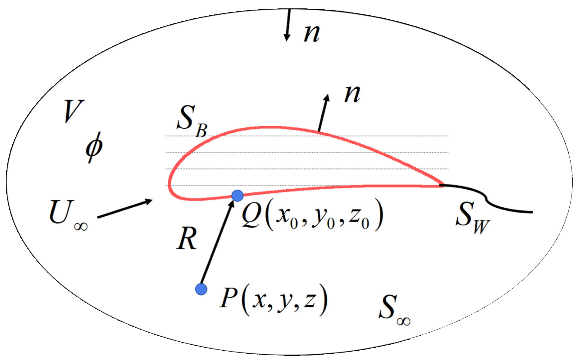
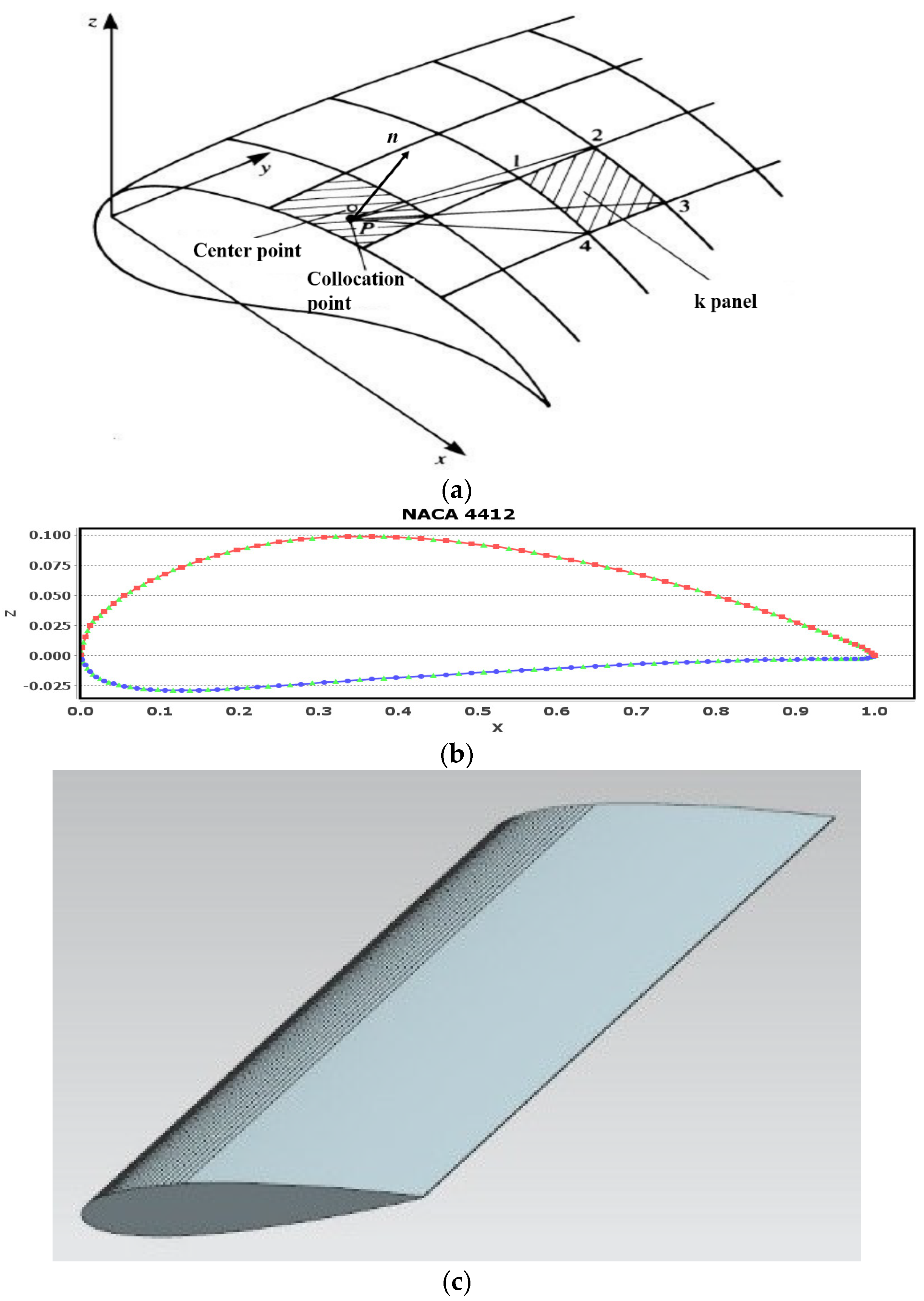
2.1. Surface Panel Method

Panel methods involve numerical models based on simplified assumptions regarding inviscid and incompressible flow problems. In principle, if a problem can be solved by distributing the unknown quantities on the boundary surface surrounding a foil under simplified potential flow, the characteristic coefficients of the foil can be obtained. Under these assumptions, the velocity vector that describes the flow field can be represented as the gradient of a scalar velocity potential. A statement of conservation of mass in the flow field leads to Laplace’s equation as the governing equation for the velocity potential. If the flow in the fluid region is considered to be incompressible and irrotational, the continuity equation can be expressed as follows [1]:

$${\nabla }^2\phi =0$$

(1)

where ${\nabla }^2$ is the Laplacian and $\varphi$ is the velocity potential. The solution of Equation (1) is based on the Green formula, a well-known function method, which can be derived from Gauss’s law and the divergence theorem. For a finite fluid domain V, the Green formula can be obtained using the divergence theorem [9]:

$${\displaystyle \underset{S}{\iint }\left(\varphi \frac{\partial \phi }{\partial n}-\phi \frac{\partial \varphi }{\partial n}\right)dS={\displaystyle \underset{V}{\iiint }\left(\varphi {\nabla }^2\phi -\phi {\nabla }^2\varphi \right)}}dV$$

(2)

where $\phi (x,y,z)$ and $\varphi (x,y,z)$ can represent any function in the finite field that has a continuous first-order partial derivative. The velocity field function in the fluid domain is represented in the calculation of the surface element, where S represents the outer boundary of the volume V and n is the outer normal vector of the boundary. By Green’s third formula for hydrofoil and propeller problems, the velocity potential at point $P(x,y,z)$ can be expressed as [32]:

$$4\pi E\varphi \left(P\right)={\displaystyle \underset{S}{\iint }\left[\varphi \left(Q\right)\frac{\partial }{\partial n}\left(\frac{1}{R}\right)-\frac{1}{R}\frac{\partial \varphi \left(Q\right)}{\partial n}\right]dS,\hspace{1em}E=\{\begin{array}{l}0\hspace{1em} P\notin V\\ 1/2 P\in S\\ 1\hspace{1em} P\in V\end{array}}$$

(3)

where Q represents the singularity point in the field and R is the distance between the collocation point P and the singularity point Q. Hence, the basic assumptions of the potential panel method for a lifting body can be illustrated as in Figure 1.

In the nonpenetrating and perturbation velocity potential attenuation conditions, the integral equation for the surface of the object can be expressed as [28,29]

$$\begin{array}{l}2\pi \varphi \left(P\right)-{\displaystyle \underset{S_B}{\iint }\varphi \left(Q\right)}\frac{\partial }{\partial n}\left(\frac{1}{R}\right)dS-{\displaystyle \underset{S_W}{\iint }\Delta \varphi \left(Q\right)}\frac{\partial }{\partial n}\left(\frac{1}{R}\right)dS\\ =-{\displaystyle \underset{S_B}{\iint }\frac{\partial \varphi \left(Q\right)}{\partial n}}\left(\frac{1}{R}\right)dS=-{\displaystyle \underset{S_B}{\iint }\frac{n\cdot \Delta \varphi \left(Q\right)}{R}}dS\end{array}$$

(4)

where $\Delta \phi$ represents the distribution of the doublet of the object’s wake surface $S_W$ and $n\cdot \nabla \phi (q)$ represents the distribution of the source of the object surface $S_B$. Equation (4) is the Fredholm integral equation of the second kind, and the velocity potential $\phi$ can be obtained from this equation. The doublet strength on the wake surface can be determined by the Kutta condition and the wake surface, and the perturbation velocity potential of the object surface can then be obtained. The perturbation velocity can be obtained by differentiating the perturbation velocity potential, and then the hydrodynamic performance can be obtained. So far, the main symbolic relationship of the above-mentioned potential flow theory is shown in Figure 1.

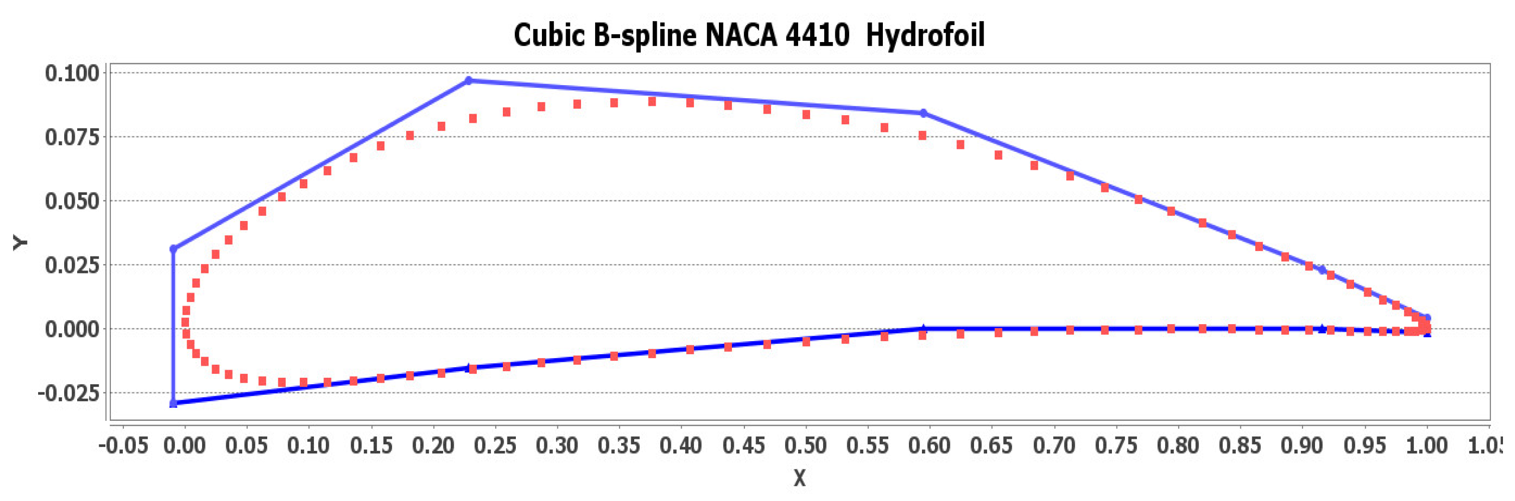
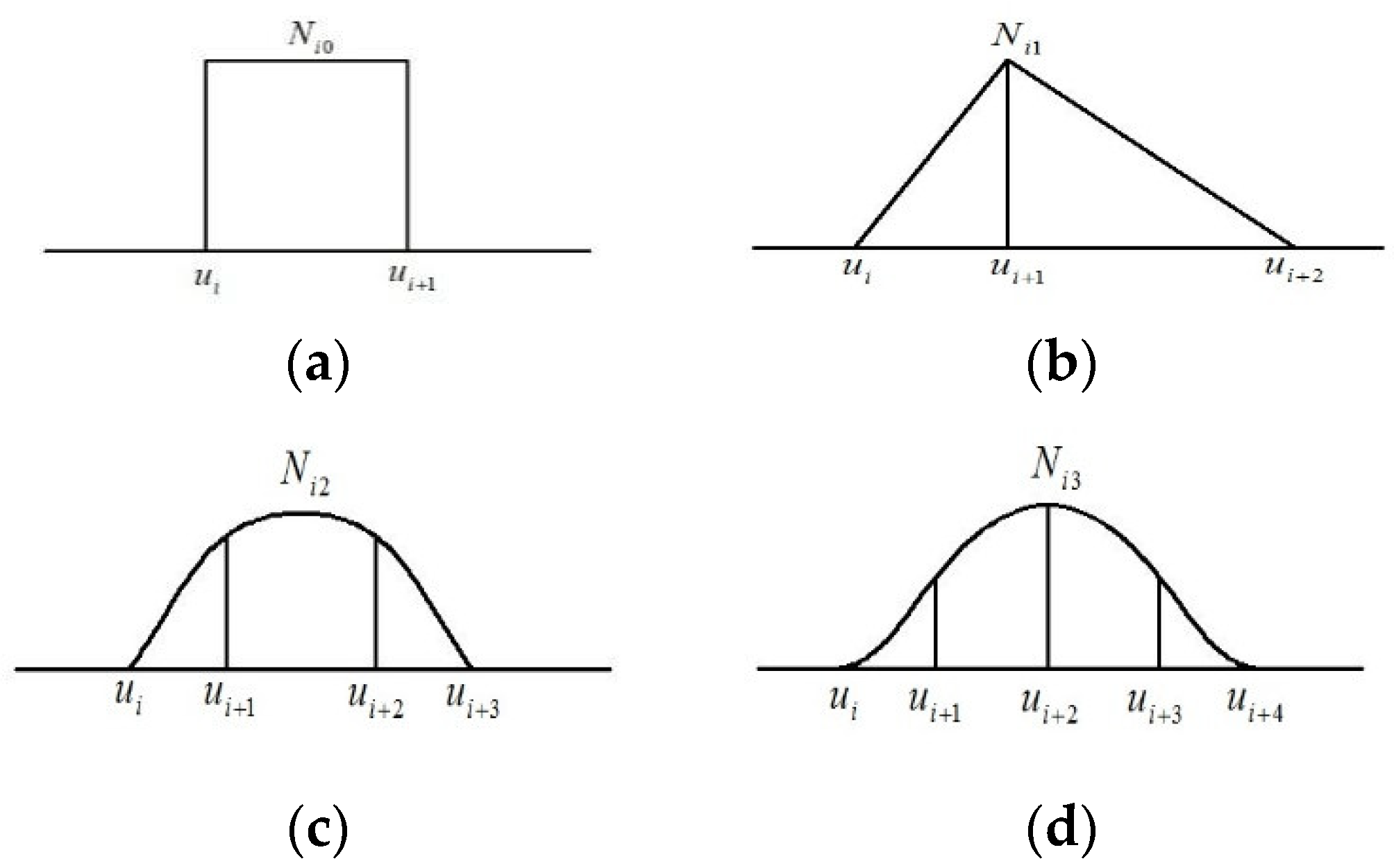
2.2. B-Spline Model Scheme

The motivation for using B-splines is to ensure that the B-spline curved panels have at least C² continuity and the B-splines can be provided with local control, i.e., changing a single point does not affect the entire curve. While natural cubic splines provide that level of continuity, they are also subject to global control, i.e., changing a single point affects the entire curve.

The B-spline curve method inherits the advantages of the Bezier curve method, preserving the basic modelling features such as defining the vertices of curves and surfaces. The B-spline curve uses a set of basic functions that is different from the one used in the Bezier curve.

The B-spline curve is expressed as follows [19]:

$$p\left(u\right)={\displaystyle \sum _{i=0}^n{d}_i{N}_{i,k}\left(u\right)}$$

(5)

where $d_i\left(i=0,1,2,\cdots ,n\right)$ is the de Boor point, which is the control point of the curve. The polygon defined by all of the control vertices is defined as the control polygon, for instance, a control polygon covering the NACA4410 hydrofoil geometry [33] can be calculated to generate a discreted cubic B-Spline curve or surface as shown in Figure 2.

In Equation (5), $N_{i,k}\left(u\right)\left(i=0,1,2,\cdots ,m\right)$ is a base function of order k. Every base function is a polynomial of order k, consisting of increasing vector nodes u. The base function can be expressed using the de Boor–Cox recursive formula [19,24] as follows:

$$N_{i,0}\left(u\right)=\{\begin{array}{l}1,\hspace{1em}\hspace{1em}{u}_i\le u\le u_{i+1}\\ 0,\hspace{1em}\hspace{1em}else\end{array}$$

(6)

$$N_{i,k}\left(u\right)=\frac{u-u_i}{u_{i+k-1}}{N}_{i,k-1}\left(u\right)+\frac{u_{i+k+1}-u}{u_{i+k+1}-u_{i+1}}{N}_{i+1,k-1}\left(u\right)$$

(7)

$$\frac{d}{du}{N}_{i,k}\left(u\right)=k\left[\frac{N_{i,k-1}\left(u\right)}{u_{i+k}-u_i}-\frac{N_{i+1,k-1}\left(u\right)}{u_{i+k+1}-u_{i+1}}\right]$$

(8)

In practice, the calculation of the entire curve is rarely performed in the application of the B-spline curve. To calculate a series of normalized B-spline basis function from Equations (6)–(8), a B-spline function of a specific order can be obtained; some of the curves are shown in Figure 3.

The number of control vertices $d_{i,j}\left(i=0,1,2,\cdots ,m;j=0,1,2,\cdots ,n\right)$ is $(m+1)\times (n+1)$, and all the control vertices constitute the control surface grid. The order of u is k, and that of v is l. The corresponding node vectors are $U=\left[\begin{array}{cccc}{u}_0,& u_1,& \cdots & ,u_{m+k+1}\end{array}\right]$ and $V=\left[\begin{array}{cccc}{v}_0,& v_1,& \cdots ,& v_{n+l+1}\end{array}\right]$. The $k\times l$ order tensor product B-spline surface can be expressed as [19]:

$$\begin{array}{l}p(u,v)={\displaystyle \sum _{i=0}^m{\displaystyle \sum _{j=0}^n{d}_{i,j}}}{N}_{i,k}(u)N_{j,l}(v)\\ u_k\le u\le u_{m+1},v_l\le v\le u_{n+1}\end{array}$$

(9)

where the basic functions $N_{i,k}\left(u\right)\left(i=0,1,2,\cdots ,m\right)$ and $N_{j,l}\left(v\right)\left(i=0,1,2,\cdots ,m\right)$ are determined by the de Boor–Cox recursion formula corresponding to the node vectors $U=\left[\begin{array}{cccc}{u}_0,& u_1,& \cdots ,& u_{m+k+1}\end{array}\right]$ and $V=\left[\begin{array}{cccc}{v}_0,& v_1,& \cdots ,& v_{n+l+1}\end{array}\right]$. For the surface problem, the inverse solution process involves calculating the inverse of the tensor product. Therefore, the inverse of the surface can be expressed by 2 inverse curves. The B-spline surface equation that needs to be inversed can be expressed as follows [19]:

$$p\left(u,v\right)={\displaystyle \sum _{i=0}^m\left[{\displaystyle \sum _{j=0}^n{d}_{i,j}{N}_{j,l}\left(v\right)}\right]}{N}_{i,k}\left(u\right)$$

(10)

where an equation similar to the curve equation [19] is constructed as given below:

$$p\left(u,v\right)={\displaystyle \sum _{i=0}^m{c}_i\left(v\right)}{N}_{i,k}\left(u\right)$$

(11)

The inverse of the applied base function is used to obtain the control vertices on the isoparametric lines. The B-spline curve is defined by the resulting control vertices. The control vertices of the required curves can be solved using the control vertices obtained as the initial points.

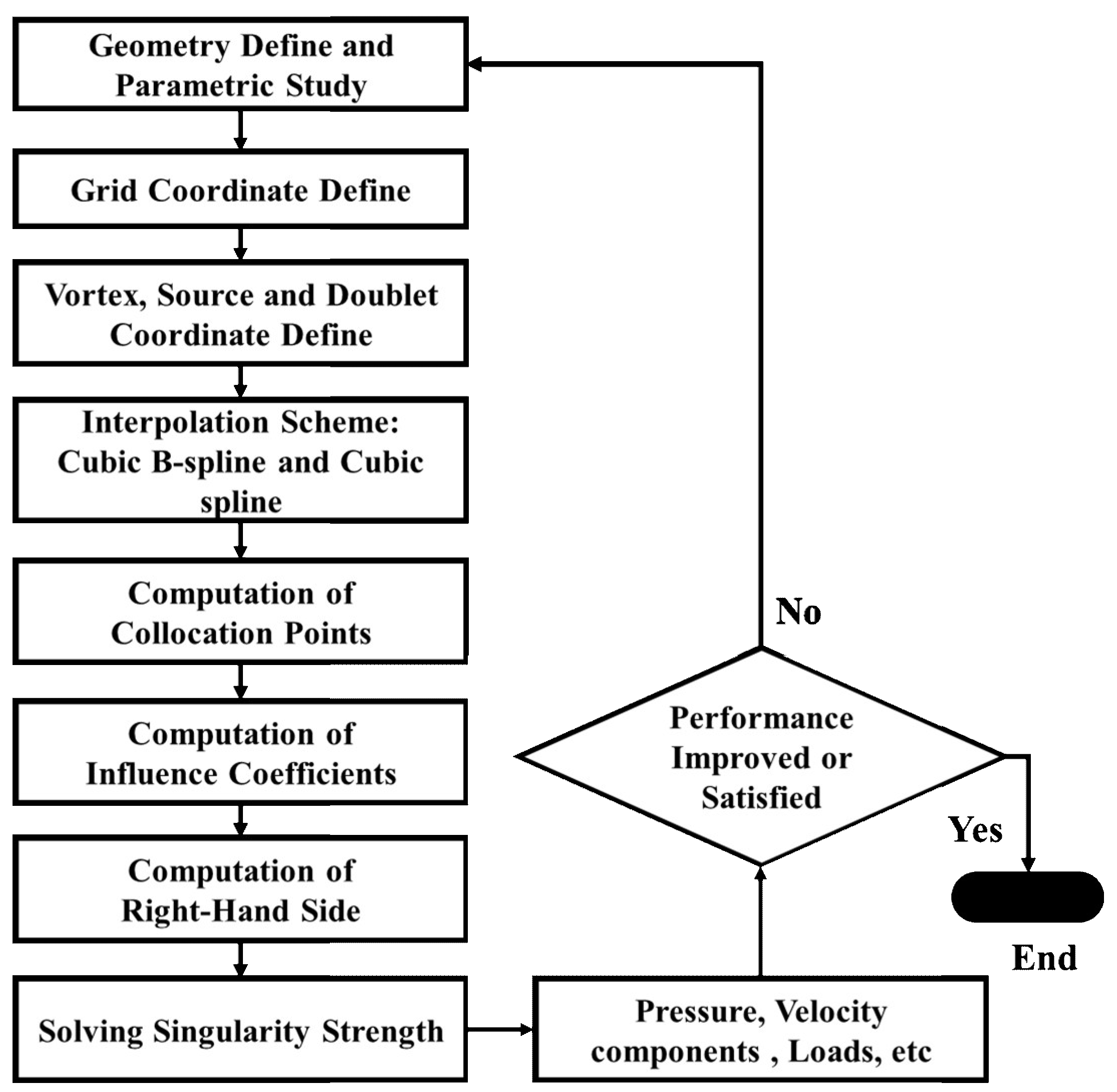
2.3. Numerical Representation of Surface Panel Method

The numerical calculation process for a surface panel method is shown in Figure 4. First, the hydrodynamic surface is defined to generate grid coordinates and points to discretize the hydrodynamic surface into N panels. Second, the number and type of singularities (solutions of the Laplace equation), such as the source, doublet, and vortex, are chosen. Third, the collocation points are placed on the curved panels to satisfy the surface-tangency condition by using the cubic B-spline interpolation scheme. Fourth, the Kutta condition is imposed and the influence of all of the singularities and the freestream at a fixed collocation point is summed. Fifth, solving the singularity strength from the system of equations generated by step 4, i.e., the zero normal flow boundary condition on each of the collocation points resulting in the set of algebraic equations as shown in Equations (12)–(14), is carried out. Finally, the estimated performance to be improved or satisfied is determined, including pressure, velocity, and load. The related numerical representation of the panel method can be referenced in Appendix A.

Modelling of 3-D Hydrofoil

The Dirichlet boundary condition is used for a hydrofoil with a certain thickness. The governing equation can be expressed as follows (the internal disturbance potential of the object is equal to zero) [28]:

$${\displaystyle \sum _{k=1}^N{c}_k{\mu }_k+{\displaystyle \sum _{l=1}^{N_W}{c}_l{\mu }_l}+{\displaystyle \sum _{k=1}^N{b}_k{\sigma }_k}=0}$$

(12)

Equation (12) is applied to every collocation point P. In the equation, l and k are the count numbers of the singularity elements. The geometry of the hydrofoil is shown in Figure 5. The influence coefficients of the doublets $c_k$, the wake doublets $c_l$, and the source $b_k$ can be calculated. The Kutta condition is expressed by the relationship between the strength of the doublets on the upper and lower surfaces and the doublet strength on the wake surface [28,32]:

$$\left({\mu }_1-{\mu }_N\right)+{\mu }_W=0$$

(13)

The matrix equation under the Kutta condition can be expressed as follows:

$${\displaystyle \sum _{i=1}^{N=1}{\displaystyle \sum _{j=1}^{N=1}{c}_{ij}{\mu }_j=\left[\begin{array}{cccccc}{c}_{11}& c_{12}& \cdots & \cdots & c_{1N}& c_{1W}\\ c_{21}& c_{22}& \cdots & \cdots & c_{2N}& c_{2W}\\ \cdots & \cdots & \cdots & \cdots & \cdots & \cdots \\ c_{N1}& c_{N2}& \cdots & \cdots & c_{NN}& c_{NW}\\ 1& 0& 0& \cdots & -1& 1\end{array}\right]}}\left[\begin{array}{c}{\mu }_1\\ {\mu }_2\\ \cdots \\ {\mu }_N\\ {\mu }_W\end{array}\right]$$

(14)

In this case, μ_w is replaced with μ_N – μ₁. Therefore, the order will be reduced to N. Only the first and the Nth columns will change because of the term ±c_iw. Hence, the influence of the doublet can be expressed as follows:

$$\{\begin{array}{ll}{a}_{ij}=c_{ij}& j\ne 1,N\\ a_{i1}=c_{i1}-c_{iW}& j=1\\ a_{iN}=c_{iN}+c_{iW}& j=N\end{array}$$

(15)

After the known matrix multiplication is moved to the right-hand side (RHS) of this equation, the RHS vector can be obtained. Based on the theory of the panel method shown above, a program based on MATLAB was developed to calculate the strength of the singularities. Then, the coefficient of pressure on the surface of the foil can be obtained. The external potential ${\varphi }_u$ can be represented as the internal potential ${\varphi }_i$ plus the doublet strength μ. Then, the local external tangential velocity component at each collocation point can be expressed by the following equations:

$${\varphi }_u={\varphi }_i+\mu$$

(16)

$$Q_t=\frac{\partial {\varphi }_u}{\partial l}$$

(17)

$$C_{pj}=1-\frac{Q_{tj}^2}{Q_{\infty }}$$

(18)

where l is the distance between 2 adjacent collocation points.

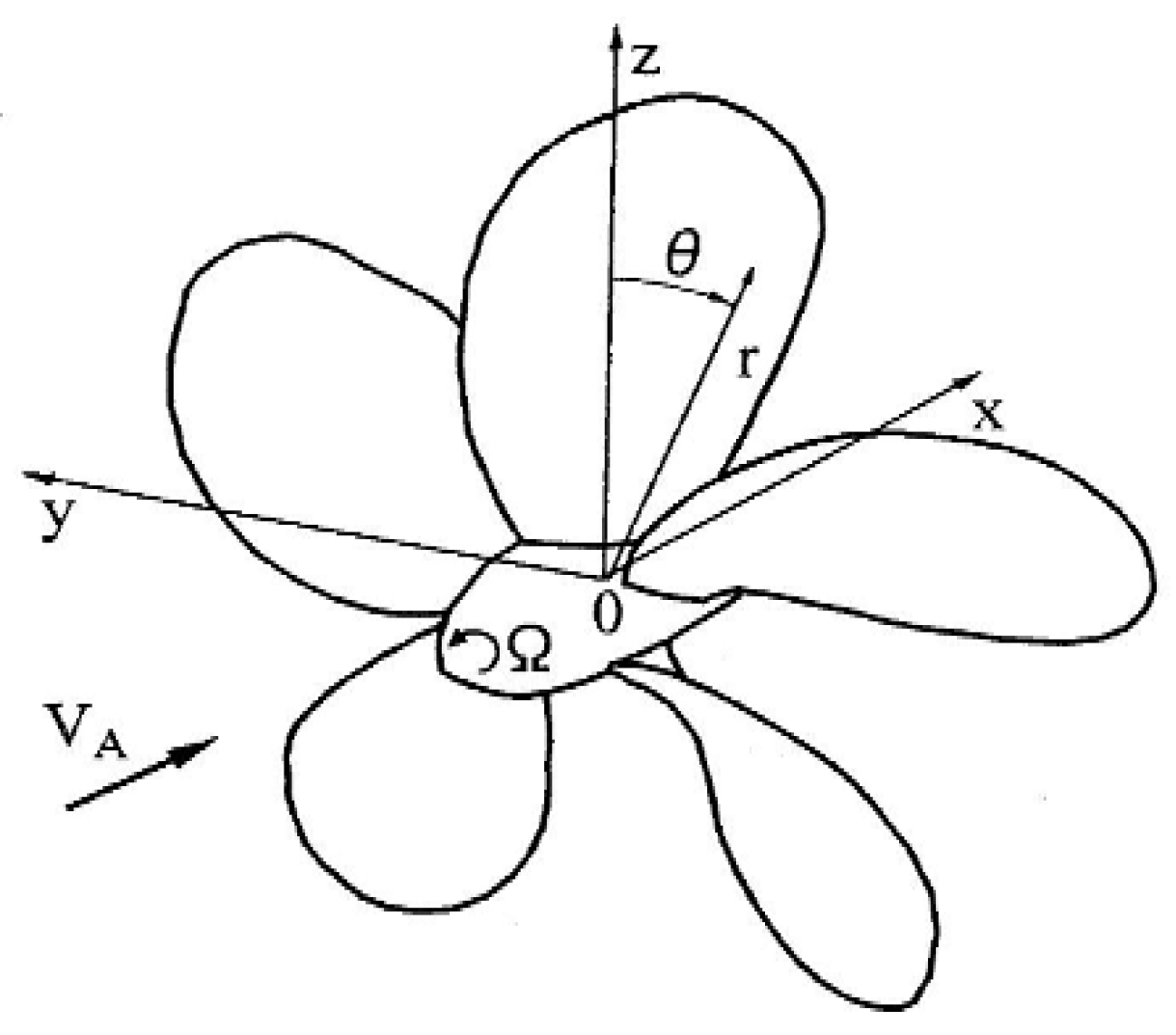
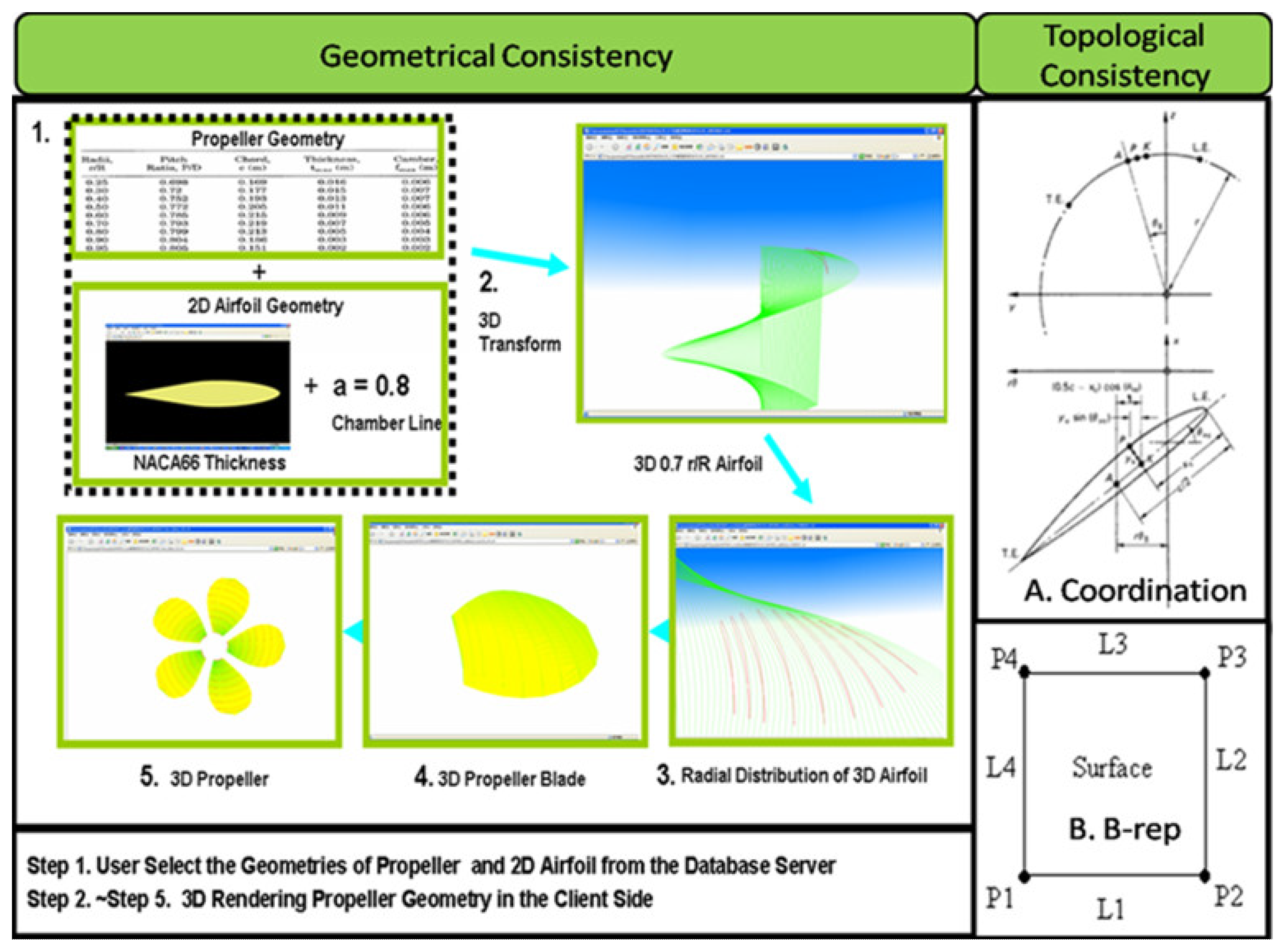
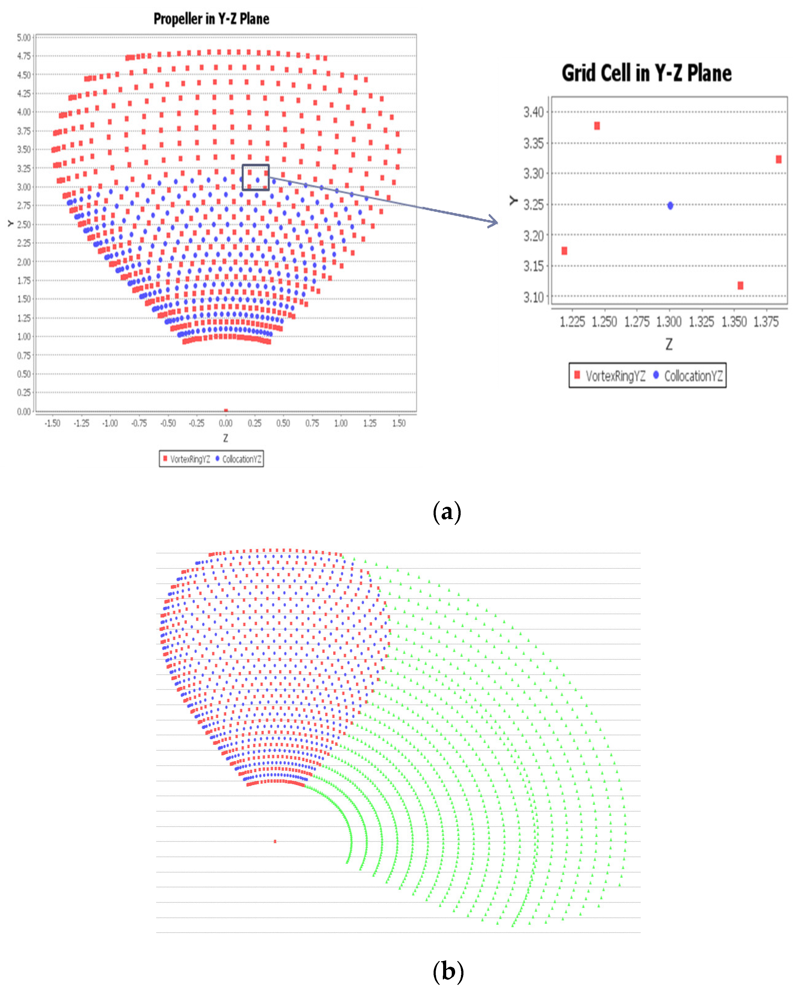
2.4. Numerical Modelling of 3-D Propeller

For geometric boundary discretization and the motion of the propeller, 2 sets of coordinate systems are established to describe the propeller geometry accurately. The rectangular coordinate system and the cylindrical coordinate system are defined as shown in Figure 6. The conversion between the 2 sets of coordinate systems is as follows [32]:

$$\{\begin{array}{l}x=x\\ y=r\cos \theta \\ z=r\sin \theta \end{array},$$

(19)

The key point in this step is the definition of the propeller coordinates. The Cartesian and cylindrical coordinates of a point on the camber surface with radial coordinate r and chordwise coordinate s can be expressed in terms of the skew (${\theta }_s$), rake ($x_m$), chord (c), and camber ($f$) [29]. With this definition, the coordinates of a point on the camber surface of the key blade can be written as [29,36]:

$$\{\begin{array}{l}{x}_c=x_m+c\left(s-1/2\right)\sin \varphi -f\cos \varphi \\ {\theta }_c={\theta }_m+c\left(s-1/2\right)\frac{\cos \varphi }{r}+f\frac{\sin \varphi }{r}\\ y_c=r\cos {\theta }_c\\ z_c=r\sin {\theta }_c\end{array},$$

(20)

The above equation expresses the coordinates of any point on the camber surface of the propeller blade. If we use $f\pm 1/2t$ to replace $f$ in the equation, we can obtain the numerical expression for the upper and lower surfaces of the propeller blade. Figure 7 shows the 3-D propeller generation process for the surface panel method.

The surface of the propeller blade is discretized using hyperbolic quadrilateral panels. Each propeller blade is divided into $N_R\times 2M_C$ panels; $N_R$ is the number of radial panels and $M_C$ is the number of spanwise panels. This method of discretization is called the cosine-clustering method. The coordinates of the corner points of the panels can be expressed as [39]:

$$\{\begin{array}{c}{r}_m=\frac{1}{2}\left[\left(1+r_h-\frac{\delta r_1}{4}\right)-\left(1-r_h-\frac{\delta r_1}{4}\right)\frac{\cos \left(\alpha +{\beta }_m\right)}{\cos \alpha }\right]\\ \alpha =\frac{\arcsin \left(\frac{\delta r_1}{\delta r_{\max }}\right)N_R-\frac{\pi }{2}}{N_R}\\ \beta =\frac{\left(\pi -2\alpha \right)\left(m-1\right)}{N_R},m=1,2,3\dots N_R+1\end{array},$$

(21)

where $\delta r_{\max }$ and $\delta r_1$ are the radial distribution of the panel with a maximum radial dimension and the first panel, respectively. At any given radius r, the propeller blade is discretized in the chordwise direction using the cosine-clustering method. From the leading edge to the trailing edge, the coordinates of the corner points are expressed as [39]:

$$\{\begin{array}{c}{s}_n=\frac{1}{2}\left(1-\frac{\cos \left(\alpha +{\beta }_m\right)}{\cos \alpha }\right)\\ \alpha =\frac{\arcsin \left(\frac{\delta s_1}{\delta s_{\max }}\right)\left(M_C+1\right)-\frac{\pi }{2}}{M_C+1}\\ \beta =\frac{\left(\pi -2\alpha \right)\left(m-1\right)}{M_C},m=1,2,3\dots M_C+1\end{array},$$

(22)

where $\delta s_{\max }$ and $\delta s_1$ are the spanwise dimensions of the panel with the maximum spanwise dimension and the first panel, respectively. The cosine-clustering method was adopted to optimize the sparse density of the discrete surfaces of the propeller panels.

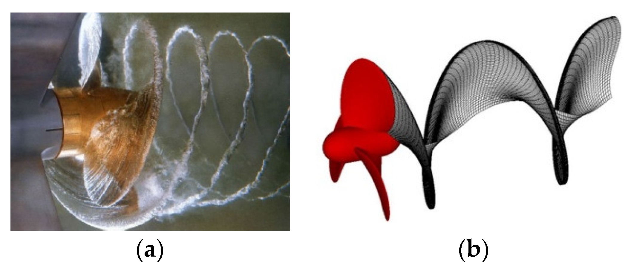
Propeller Wake Model

The propeller wake model has an influence on the perturbation velocity potential flow of the propeller. The helical spiral surface can be used to model the wake surface of a propeller. The propeller pitch angle can be expressed by a linear combination of the blade pitch angle and that based on lift-line theory. Greeley and Kerwin [36] proposed a model of radial shrinkage in the wake region and achieved good results. In this wake model, the radius of the wake surface decreases and eventually shrinks into 2 vortices, the hub vortex and the tip vortex. Kanemaru and Ando [16] improved the geometry of the wake surface by making it more refined, combining Gaschler’s experimental results [40] on the wake surface into the modelling.

In this study, a wake shrinkage model was applied to improve the prediction of the performance of a propeller in which the pitch of the wake surface changes with shrinkage (Figure 8). To obtain a more reasonable panel distribution on the wake surface, the discrete coordinates of the wake surface can be calculated using Equations (21)–(25). Specifically, when a downstream coordinate is given, the region from the blade to the downstream coordinate ${\theta }_w$ is the near-wake region, and the region farther than the downstream coordinate ${\theta }_w$ is the far-wake region. The distance from the angular coordinate ${\theta }_{TE}$ of the trailing edge to the downstream coordinate ${\theta }_w$ is defined by s, and the radius of the wake is contracted to $r_w$ at $s=1$. It is assumed that the wake radius of the central part changes smoothly, and that the pitch angle of the wake surface changes smoothly in the direction of the blade radius and wake flow. The radius of the far-wake region at $s>1$ does not shrink, while the pitch angle does not change in the direction of the wake flow. The geometric parameters of the wake surface are defined as follows:

(1) Tip vortex radius [39]:

$$r_{tip}\left(s\right)=\{\begin{array}{ll}{r}_{TE}^{}+\left(r_w-r_{TE}\right)\cdot \left(3s-3s^2+s^3\right)& 0\le s\le 1\\ r_{rw}& s>1\end{array}$$

(23)

(2) Wake radius at other locations [41]:

$$r\left(s\right)=\{\begin{array}{ll}\sqrt{r_h^2+\left(r_{TE}^2-r_h^2\right)\cdot \left(\frac{r_{tip}^2\left(s\right)-r_h^2}{r_{tip}^2\left(s\right)-r_h^2}\right)}& 0\le s\le 1\\ C_{rw}=0.625+0.05{\theta }_s{/90}^{\circ }& s>1\end{array}$$

(24)

where $r_{TE}$ represents the blade radius at the trailing edge, $r_h$ represents the radius of the propeller hub, and $r_w$ represents the radius of the shrinking tip vortex and satisfies the following conditions [29,31]:

$$\{\begin{array}{l}{r}_w=C_{rw}+\frac{J}{P_{0.7R}/D}\left(0.475-0.255\frac{J}{P_{0.7R}/D}\right)\\ C_{rw}=0.625+0.05{\theta }_s{/90}^{\circ }\end{array}$$

(25)

The pitch angle of the wake surface changes as the following equation [39,42]:

$${\beta }_w\left(s\right)=\{\begin{array}{ll}{\beta }_w\left(0\right)+\left({\beta }_w\left(1\right)-{\beta }_w\left(0\right)\right)\cdot \left(3s-3s^2+s^3\right)& 0\le s\le 1\\ {\beta }_w\left(1\right)={\beta }_G\left(r\right)& s>1\end{array}$$

(26)

Figure 9 shows discrete panels on a propeller and wake surface for the surface panel method. The geometric model of the wake surface can be constructed accurately using the characteristic quantities of the wake surface. Because the influence of the panels at the trailing edge is greater, the cosine-clustering method was applied for the wake surface at a given radial profile. The corner point coordinates of the panels in the wake transition region were determined using the following equation [37]:

$$\{\begin{array}{l}\theta \left(s\right)={\theta }_{TE}+s\left(i\right)\cdot \left({\theta }_w-{\theta }_{TE}\right)\\ s\left(i\right)=\frac{1}{2}\left(1-\cos \frac{i-1}{N_w}\pi \right),i=1,2,\cdots ,N_w+1\end{array}$$

(27)

3. Results

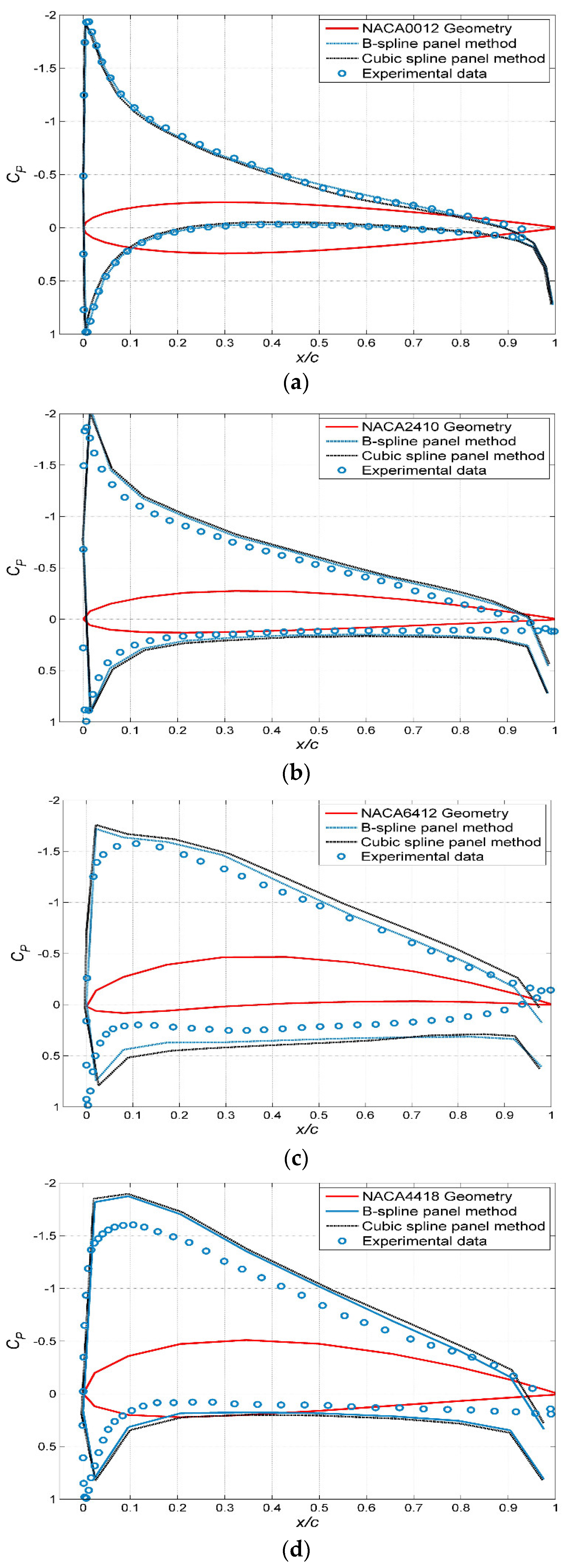
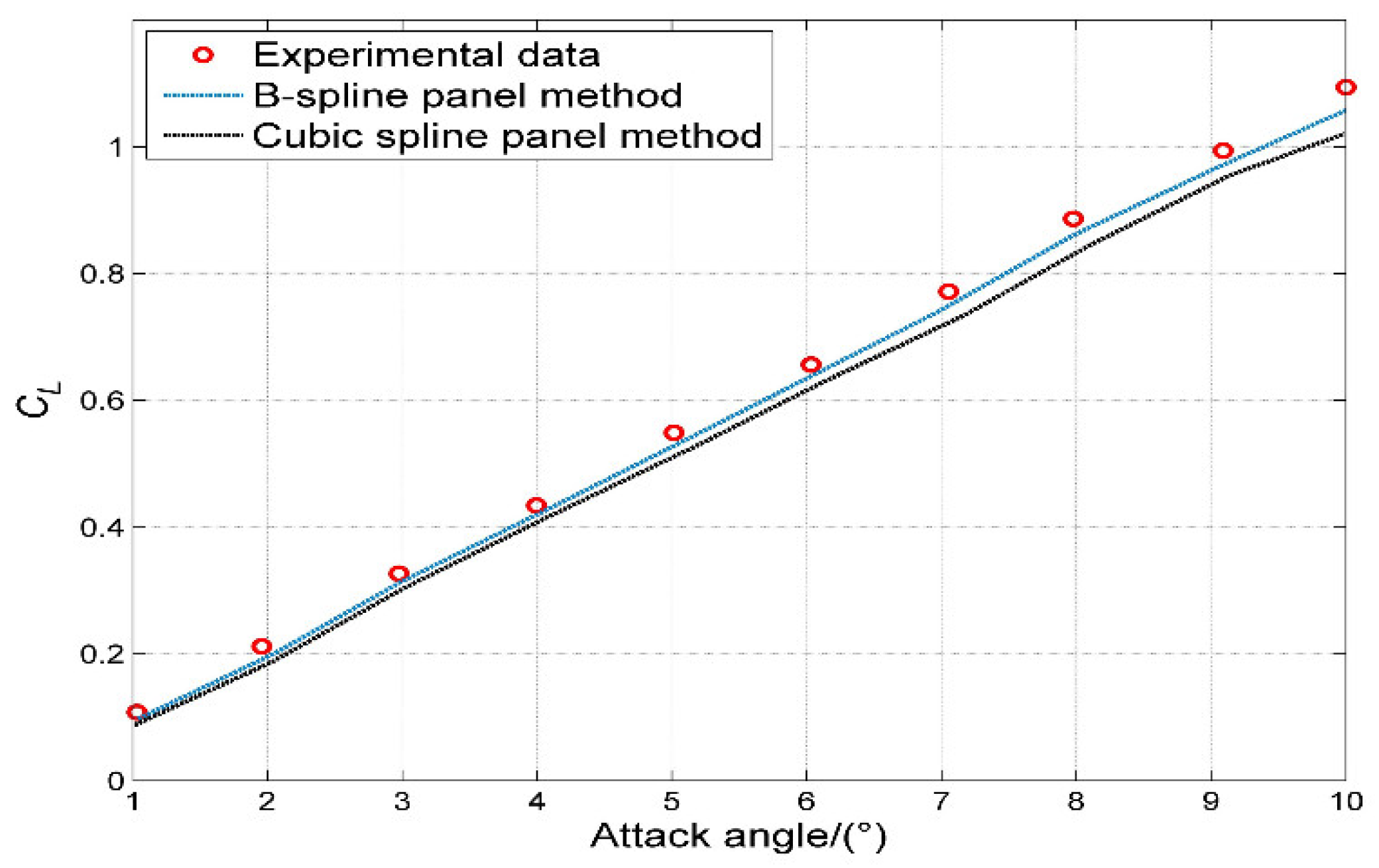
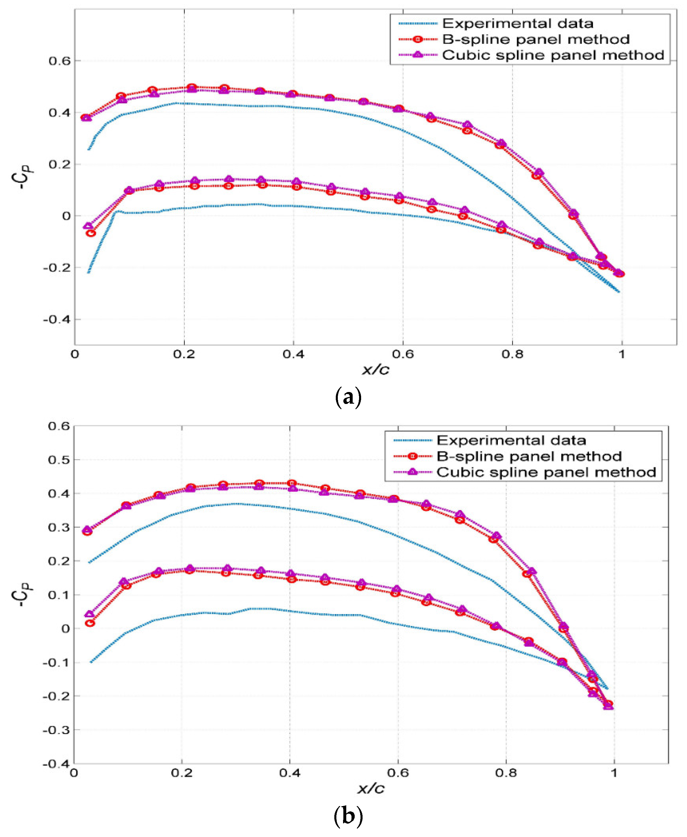
3.1. Validation of the Panel Method Using 2-D Hydrofoil Performance

To validate the two-dimensional hydrofoil panel method, the hydrofoil profiles NACA0012, NACA2410, NACA6412, and NACA4418 [33] were selected for calculation. The lift coefficient of NACA0012 was calculated at different angles of attack using the two-dimensional hydrofoil panel method and compared with the experimental data; the results are shown in Figure 10a–d.

Figure 10a–d show that the calculated results are in good agreement with the experimental data [33], and the average error using the B-spline panel method is within 6.3% whereas the average error was 7.1% using the cubic spline panel method. The results for NACA0012 and NACA2410 have the highest degree of agreement. There are some differences between the calculated results and experimental data for NACA6412 and NACA4418, but the trend of the pressure coefficient curve obtained through calculation is in good agreement with the experimental data [33]. The higher the degree of the camber line, the greater the effect on the calculation accuracy; the number of panels also has some influence on the calculation results. For the two-dimensional hydrofoil, the number of panels should be controlled in the range of 40–80. A lower grid density would lead to less accuracy. Figure 11 shows a comparison of the calculated and experimental results of lift coefficient for NACA0012 at different angles of attack using the B-spline and cubic spline panel methods. The calculated results using the B-spline panel method show a higher degree of agreement with the experimental data.

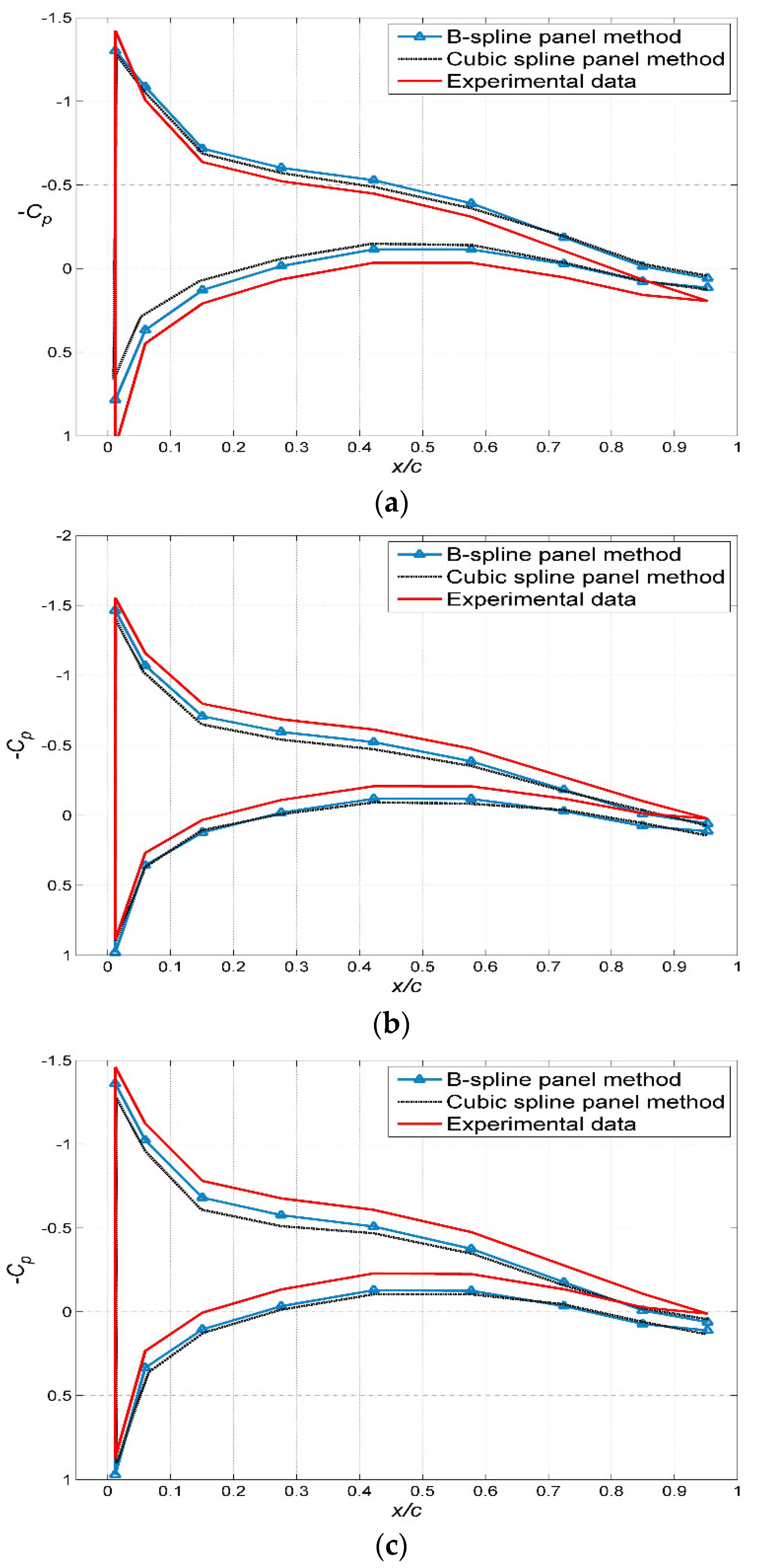
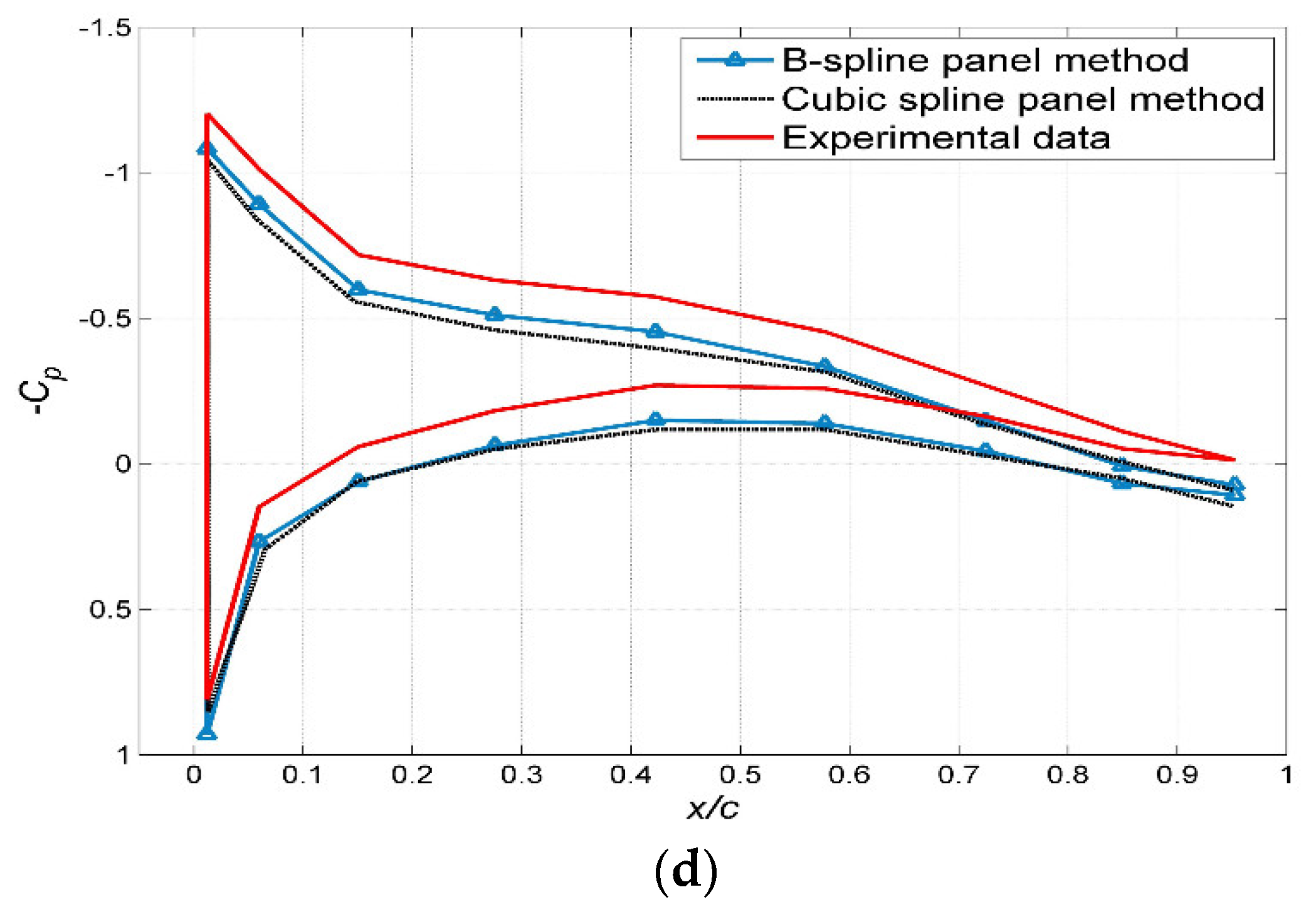
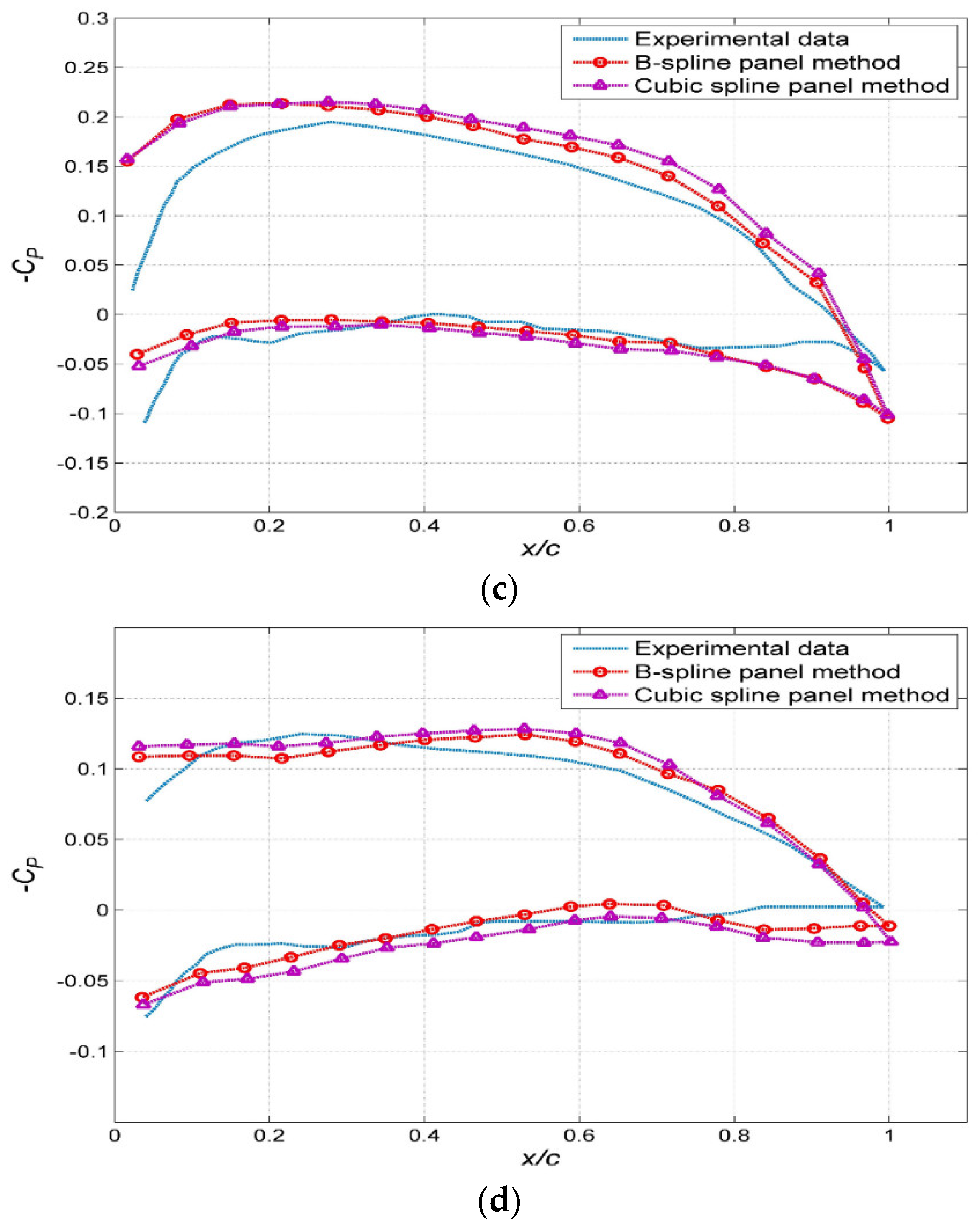
3.2. Validation of the Panel Method Using 3-D Hydrofoil Performance

In this study, a three-dimensional rectangular hydrofoil was selected for calculation using the panel method. The hydrofoil type selected was NACA0012 [33]. The aspect ratio was set to 10, the angle of attack was set to 5°, and the number of panels was 180. The surface pressure distribution on the hydrofoil is shown in Figure 12.

The surface pressure distribution of the hydrofoil can be directly compared with the experimental data reported by Lee and Jang [34]. In the present study, the number of chordwise panels per section is 18, and the number of spanwise panels per section is 10. With this discretization method, it is possible that some regions of the panel shape become relatively slender, resulting in a lower calculation accuracy. It is necessary to develop some algorithm to judge the size of the panels to ensure that they are not very slender. The results obtained using the hydrofoil panel method are compared with the experimental results for the sections defined by a span fraction (s) to the wing span (S) as s/S = 0.25, 0.5, 0.65, and 0.85 as shown in Figure 13a–d, respectively.

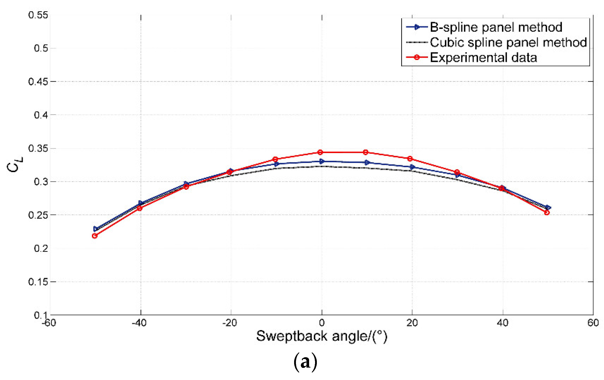
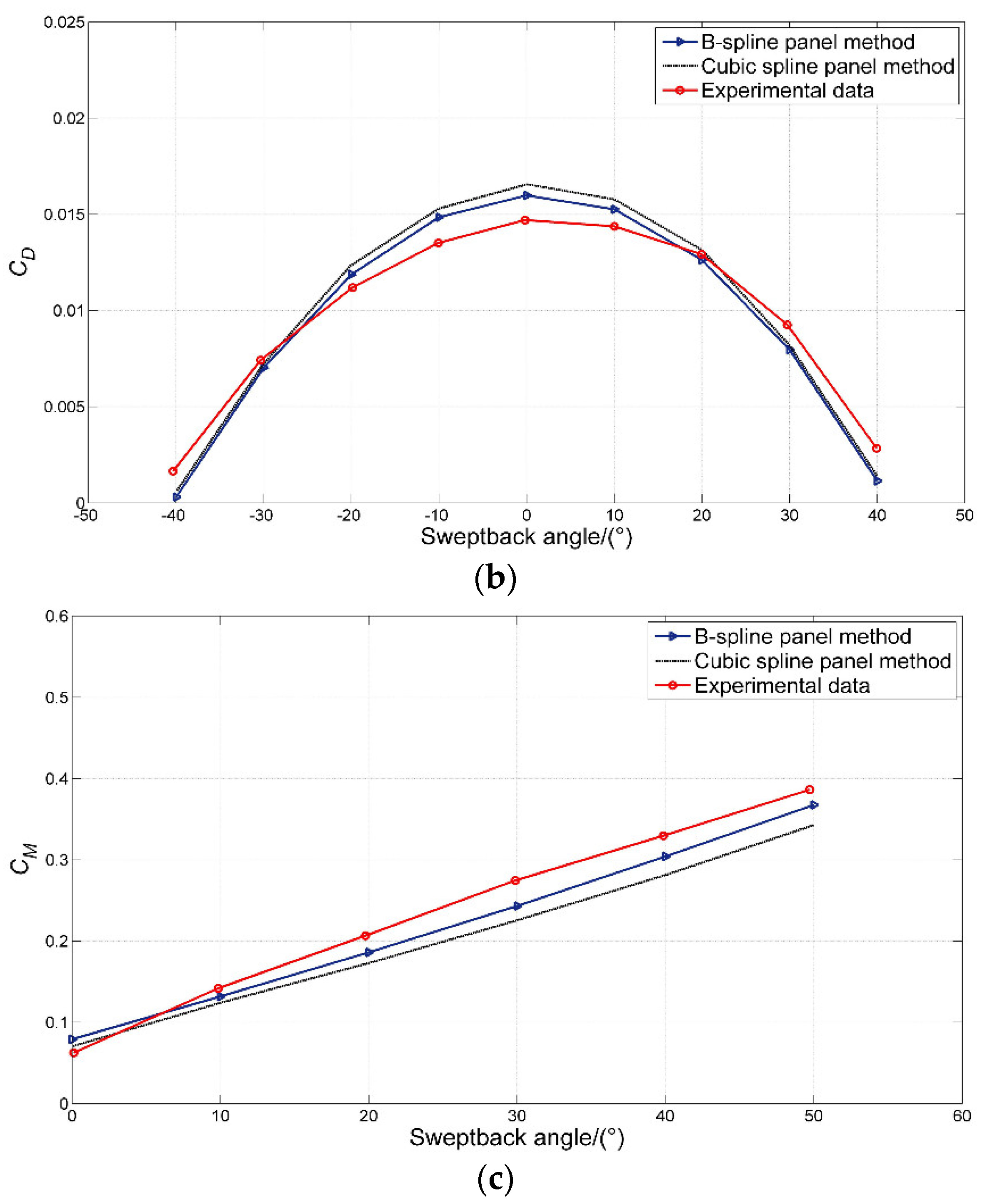
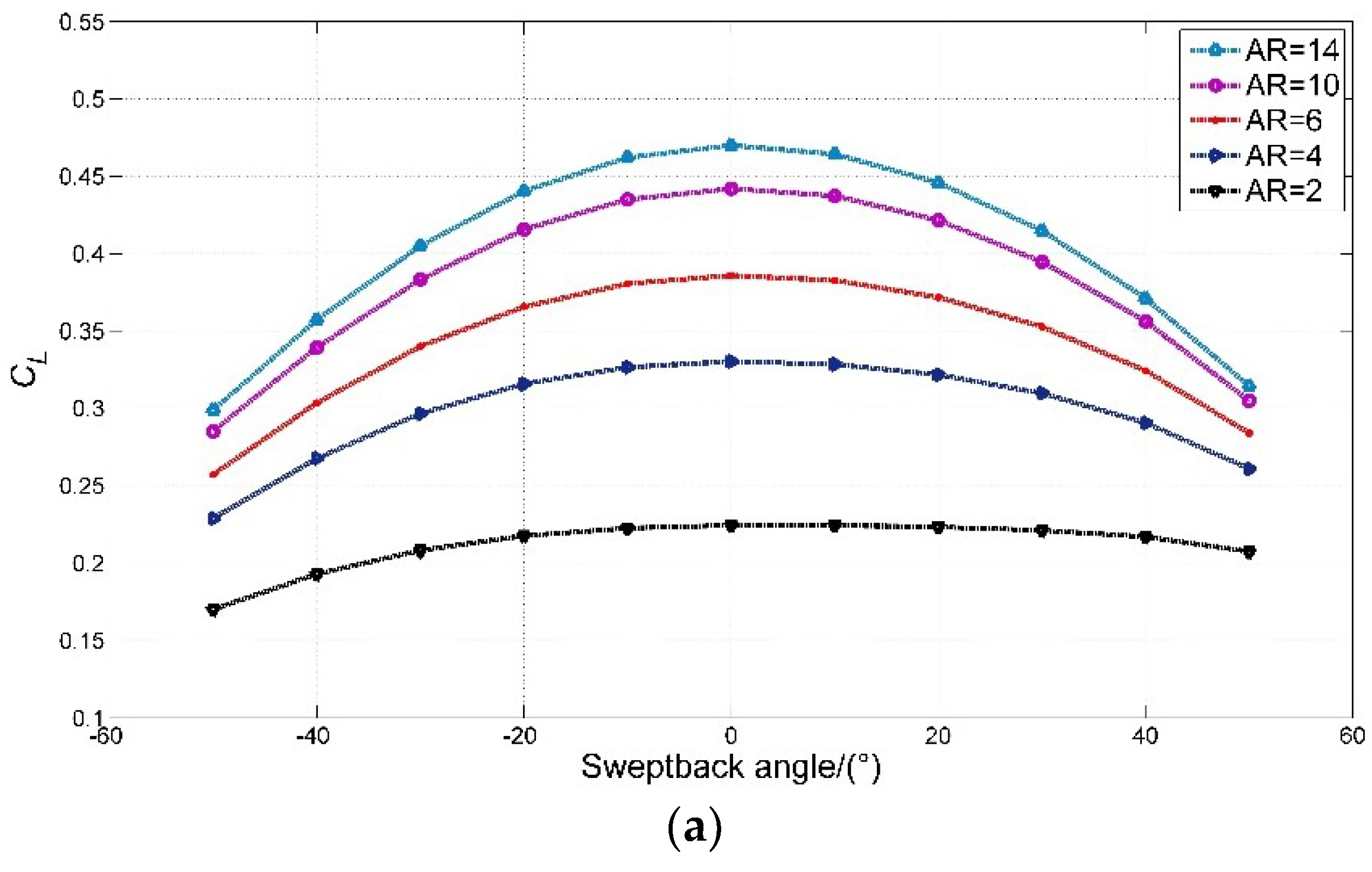
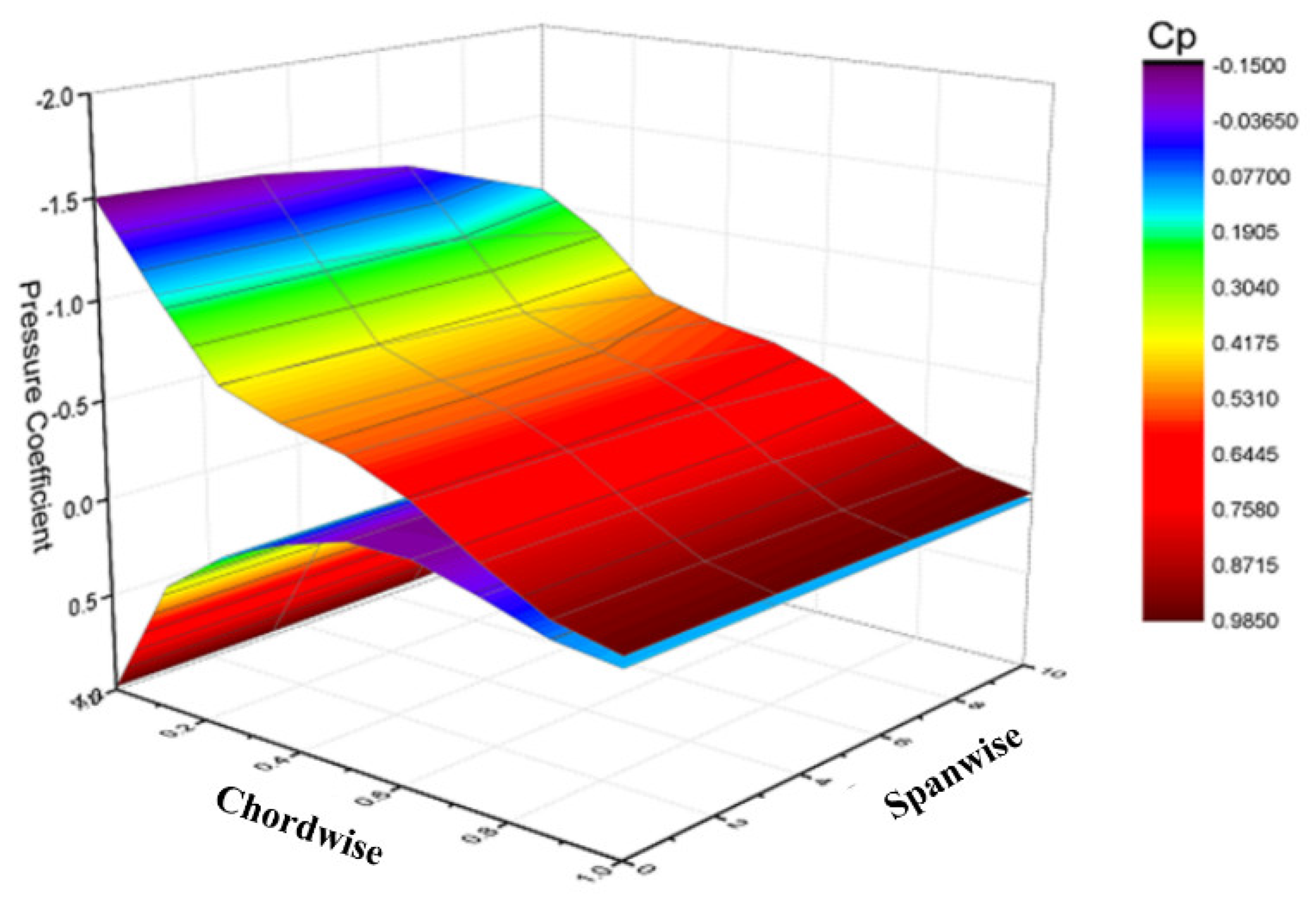
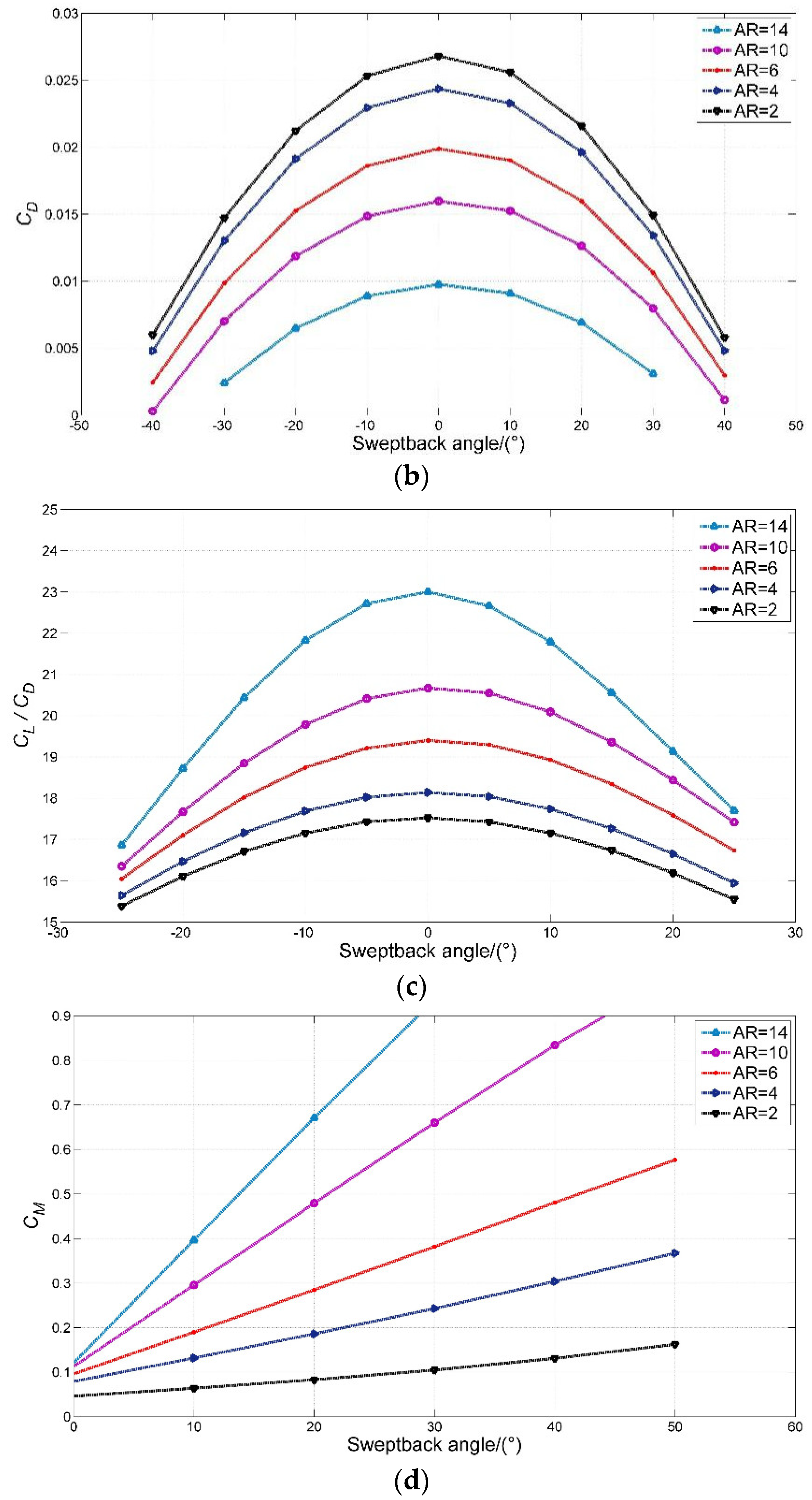
3.3. Hydrodynamic Analysis of Sweptback and Sweptforward Hydrofoils

Compared with the straight rectangular hydrofoil, the sweptback hydrofoil can effectively reduce the impact force of the flow and improve the hydrodynamic performance. To test the adaptability and stability of the panel method, rectangular hydrofoils with different sweptback and sweptforward angles were selected for analysis. The hydrodynamic performance was calculated with different sweepback angles at a limited angle of attack using the panel method. Discretization of the hydrofoil was performed using the cosine-clustering method. The aspect ratio was set to 6 and the angle of attack was set to 5°. A comparison of the calculation results and the experimental data of the sweptback hydrofoil performance [41] is given in Figure 14. The experimental data considered the ground effect on the sweptback hydrofoils whereas the prediction of the sweptback hydrofoil performance in the present panel method did not consider the ground effect, hence, the value of the experimental lift coefficient at the zero sweptback angle is greater than those of the panel methods as shown in Figure 14a.

Figure 14a–c show that the lift coefficients, induced drag coefficients, and moment coefficients calculated by the B-spline and cubic spline panel methods are in good agreement with the experimental data. The average error based on the cubic B-spline method is within 4% whereas the cubic spline one is 5.9%. The calculated results using the B-spline panel method show a higher degree of agreement with the experimental data. Hence, a better superiority was experienced in the cubic B-spline panel method compared to the cubic spline one. The lift coefficient and induced drag coefficient of the hydrofoil reach the maximum value when the sweptback angle is near zero and decrease with the increased sweep angle. A comparison of the calculation results of hydrofoil performance with different aspect ratios based on the cubic B-spline panel method is given in Figure 13 and Figure 15.

Figure 15a–d show that the lift coefficient and the lift-to-drag ratio increase with the increased aspect ratio of the sweptback hydrofoil, while the induced drag coefficient and moment coefficient decrease.

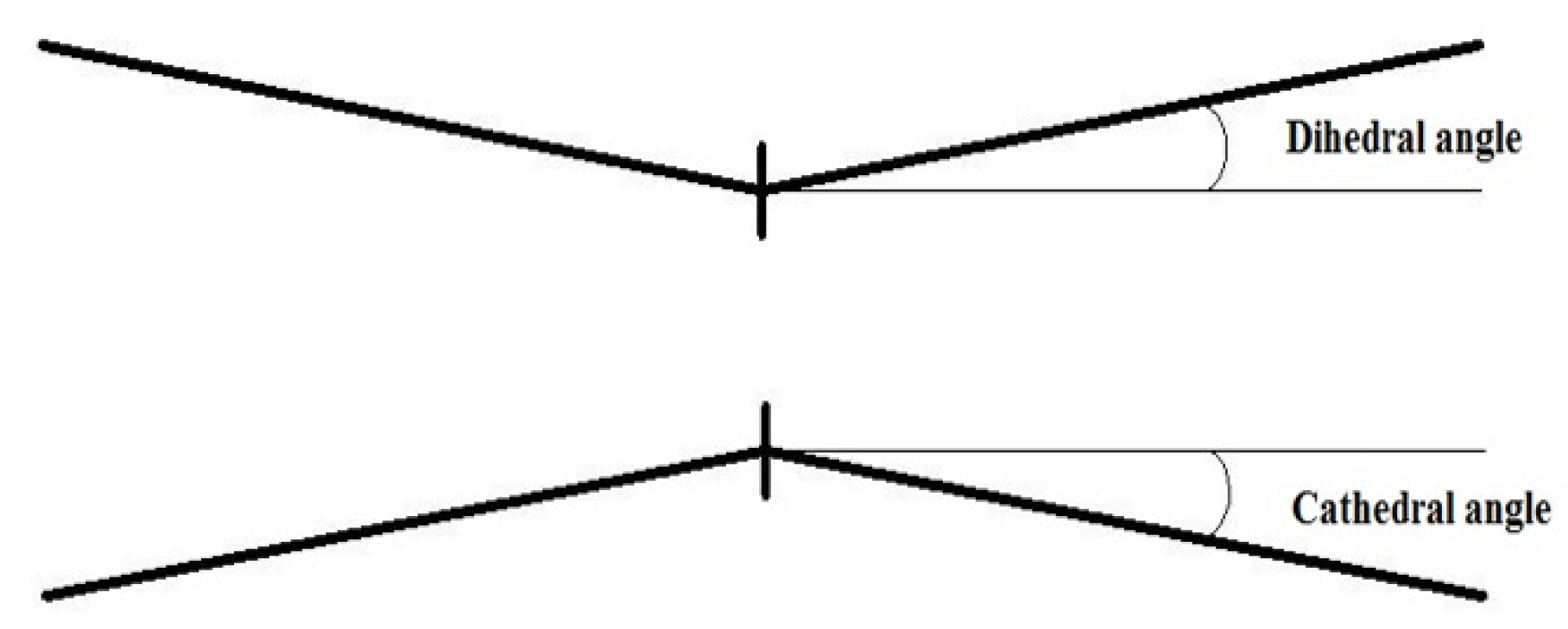
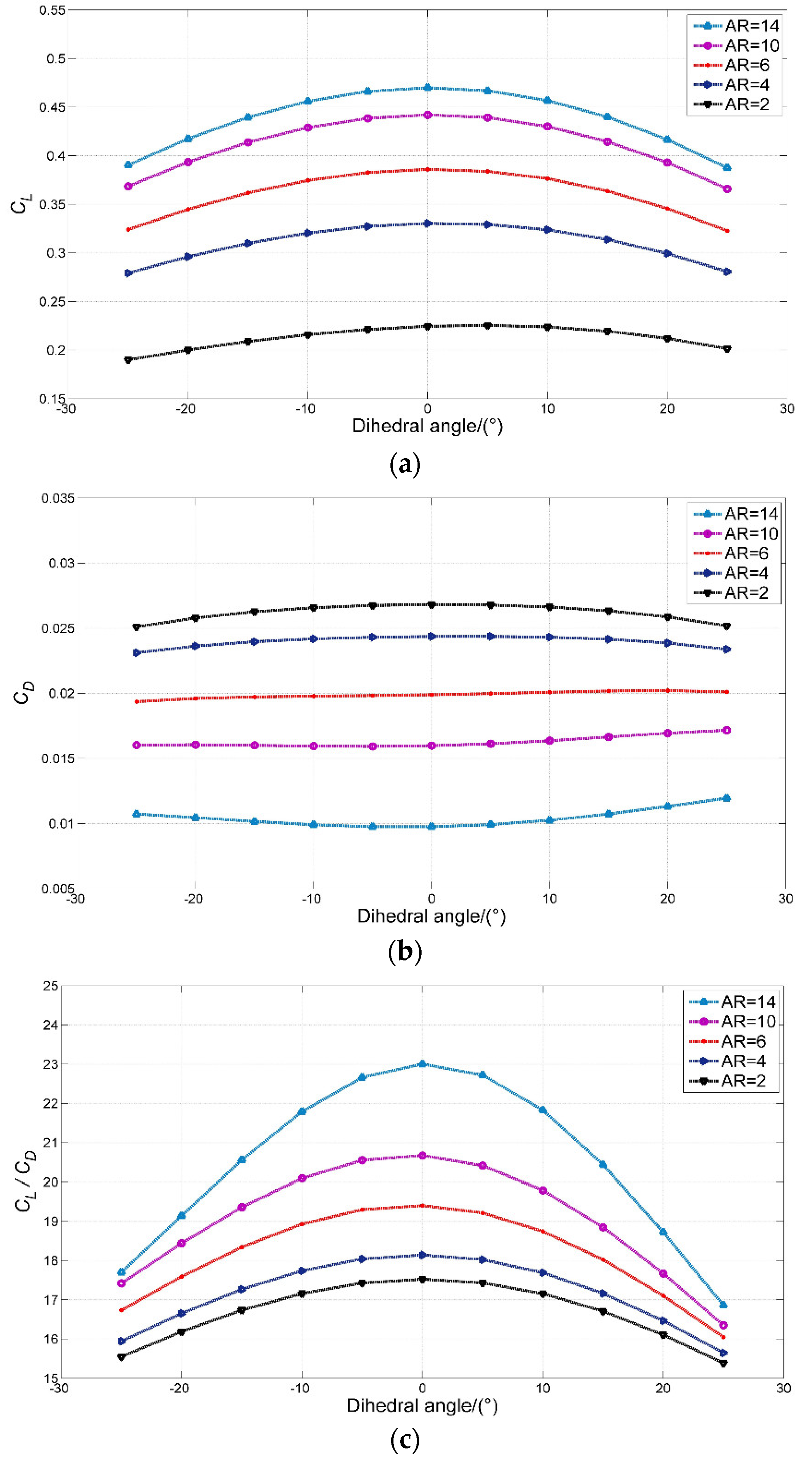
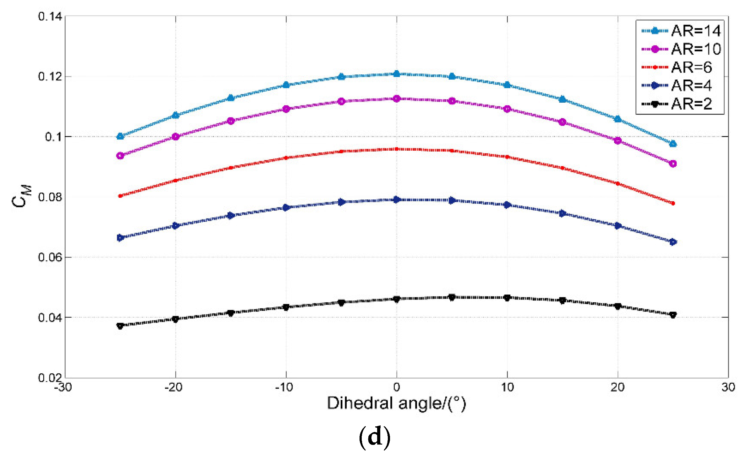
3.4. Hydrodynamic Analysis of Dihedral Hydrofoils

The stability of the hydrofoil can be improved by using a dihedral hydrofoil as shown in Figure 16. The calculation results of the hydrodynamic performance of the dihedral hydrofoil with different aspect ratios based on the cubic B-spline panel method are shown in Figure 17.

Figure 17a–d show that with the increased dihedral angle, the lift coefficient, lift-to-drag ratio, and moment coefficient decrease, and the induced drag coefficient changes with the aspect ratio.

For low-speed hydrofoils, the hydrodynamic performance can be improved by increasing the lift coefficient and the lift-to-drag ratio; in this case, it is possible to increase the hydrofoil aspect ratio, reduce the sweptback angle, and keep the hydrofoil as straight as possible. At higher speeds, the hydrofoil must not only have a good hydrodynamic performance, but it may also be resistant to stress fatigue; hence, it is not appropriate to reduce the aspect ratio and increase the sweptback angle.

3.5. Results of Propeller Performance

In this study, the DTMB series propellers with different values of rake and skew were selected for calculation of hydrodynamic performance using the panel methods with the present method and the conventional cubic spline scheme. The selected propellers were DTMB4119, DTMB4497, DTMB4498, DTMB4381, DTMB4382, DTMB4383, and DTMB4384.

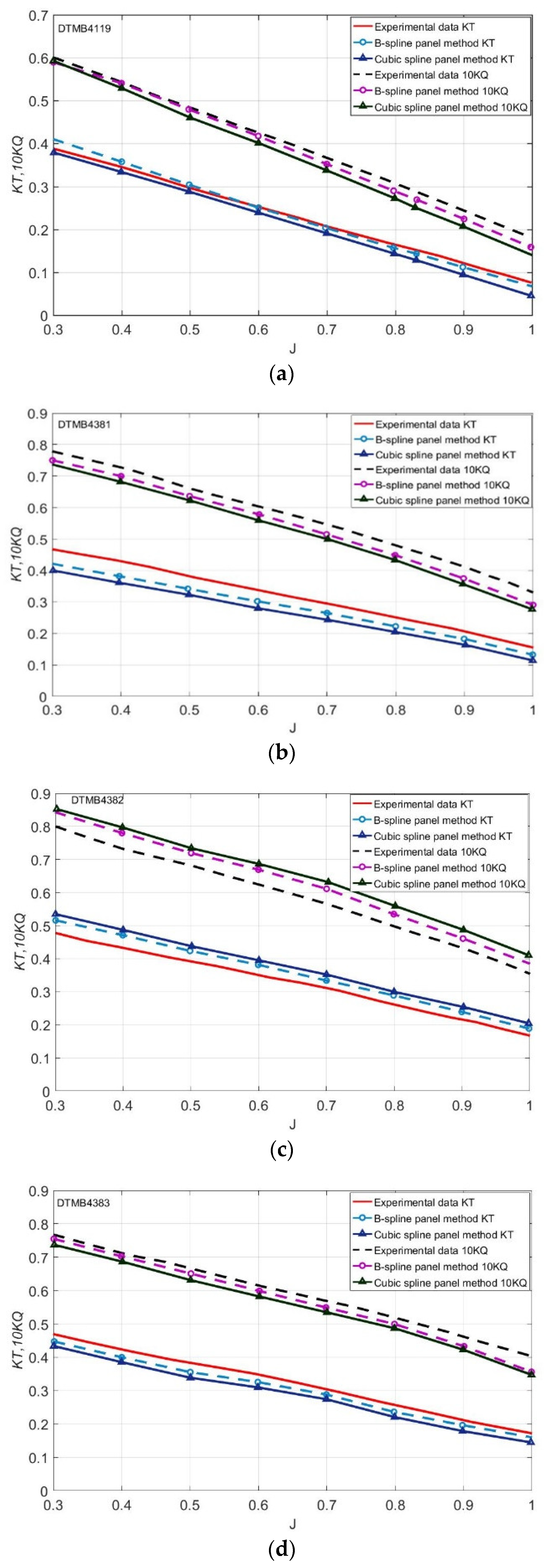
3.5.1. Validation of the Panel Method Using DTMB4119 Propeller Performance

DTMB4119 was approved by the 20th International Towing Tank Conference as a standard propeller to verify the accuracy of the panel method. The geometric parameters of the propeller and the experimental data pertaining to DTMB4119 were taken from the conference reports [2,37], and the corresponding details for the other propellers were taken from previously published documents [29,36,43].

The propeller blade surface was discretized in the chordwise direction using the cosine-clustering method. The DTMB4119 propeller panel discretization model is shown below (Figure 18) and the relative characteristics of the DTMB4119 are shown in

Table 1. The geometric parameters of propeller DTMB4119 [37].

Number of blades, Z: 3 Hub diameter ratio: 0.2 Expanded area ratio: 0.6 Section mean line: NACA a = 0.8 Section thickness distribution: NACA66 (modified) Design advance coefficient, J = 0.833
r/R	c/D	P/D	${\mathit{\theta }}_{\mathit{s}}$	${\mathbf{x}}_{\mathbf{m}}/\mathbf{D}$	$\mathbf{t}/\mathbf{D}$	${\mathbf{f}}_{\mathbf{0}}/\mathbf{c}$
0.200	0.321	1.105	0	0	0.200	0.014
0.250	0.343	1.103	0	0	0.180	0.019
0.300	0.361	1.102	0	0	0.161	0.023
0.400	0.405	1.098	0	0	0.113	0.023
0.500	0.443	1.093	0	0	0.093	0.021
0.600	0.463	1.087	0	0	0.074	0.020
0.700	0.465	1.083	0	0	0.052	0.020
0.800	0.436	1.081	0	0	0.043	0.019
0.900	0.363	1.078	0	0	0.032	0.018
0.950	0.286	1.077	0	0	0.034	0.016
1.000	0.031	1.075	0	0	0.001	0

[37].

The literature [2,37] offers the experimental data of the pressure coefficient distribution for DTMB4119 at different sections at a speed factor of J = 0.833. A comparison of the pressure coefficients obtained from the experimental data and the calculated results is shown in Figure 19a–d.

In general, the calculated results of the surface pressure coefficient of the DTMB4119 propeller blade are in agreement with the experimental results [2,37], and the average error is within 7.3%. The selection of the wake model has some influence on the calculation results. The model selected in this study is the empirical wake model, which is different from the actual wake. Therefore, the wake model is not the main factor in the calculation results.

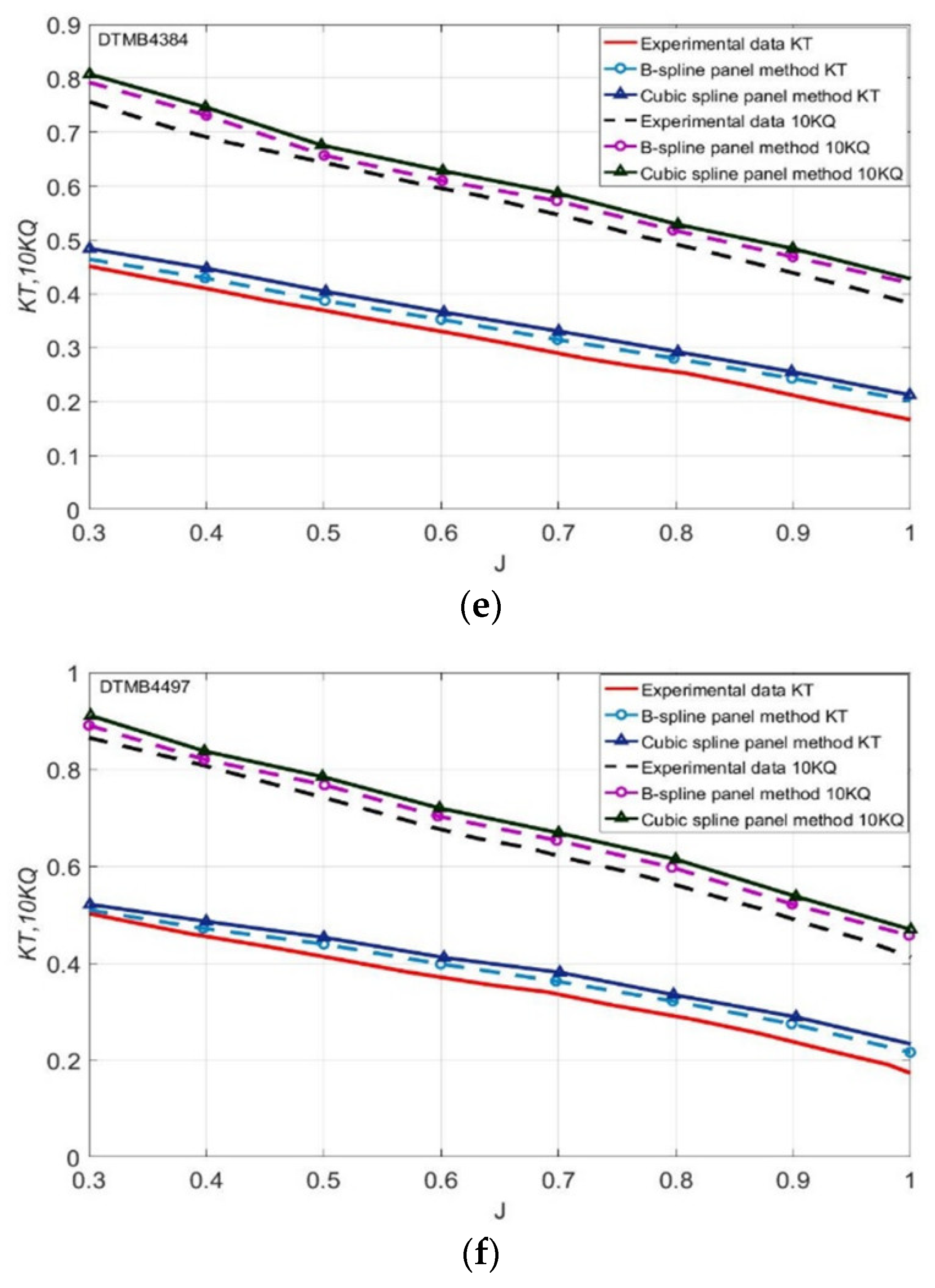
3.5.2. Results of Propeller Thrust and Toque

A comparison of the hydrodynamic coefficients for the propellers obtained from the calculation results and experimental results [2,36,38] is shown in Figure 20a–f. The number of panels is 280. Based on the cosine clustering method together with cubic B-spline interpolation, these panels were clustered more tightly and smoothly near leading and trailing edges of 3-D propeller hydrofoils placed on the propeller helix lines for the best results.

Figure 20a–f show that the hydrodynamic performance of the propellers is in good agreement with the experimental data, and the average error is within 7.3% based on the cubic B-spline panel method whereas the average error 8.2% using the conventional cubic spline panel method. Especially for the DTMB4119 propeller, the accuracy of the hydrodynamic performance calculation is high, and the average error is within 6% based on the proposed method.

4. Conclusions

A computational technique using the B-spline panel method and the cubic spline panel method to predict the performance of a hydrofoil and propeller is presented in this paper. The surface pressure coefficient and lift performance of a two-dimensional hydrofoil are calculated and analyzed by the above numerical methods. The results are compared with the experimental data. In addition, the hydrodynamic performance of a three-dimensional hydrofoil and of a sweepback hydrofoil and a dihedral hydrofoil with different aspect ratios are analyzed, and the average error is within 4% in the present method, whereas it is 5.9% of the cubic spline method. The results confirm the rationality and feasibility of the method. The surface pressure distribution and the coefficients of thrust and torque of different propellers are calculated and compared with the experimental data, and the average error is within 7.3% in the present method whereas it is 8.2% using the conventional method. The comparison results are found satisfactory. In conclusion, the validity of all the calculated results from the cases studied in this paper was proved by comparing them to the available studies in the literature. Additionally, the calculated results using the proposed B-spline panel method show a higher degree of agreement with the experimental data than the cubic spline one. In the future, the panel method can be used for the inverse design based on the required load and modelling predictions of hydrofoil cavitation.

References

1. Hess, J.L.; Smith AM, O. Calculation of potential flow about arbitrary bodies. Prog. Aerosp. Sci. 1967, 8, 1–138. [Google Scholar] [CrossRef]
2. Brandner, P. Calculation Results for the 22nd ITTC Propulsor Committee Workshop on Propeller RANS/PANEL Methods Steady Panel Method Analysis of DTMB 4119 Propeller. Available online: https://www.researchgate.net/publication/237730350_Calculation_Results_for_the_22nd_ITTC_Propulsor_Committee_Workshop_on_Propeller_RANSPANEL_Methods_Steady_Panel_Method_Analysis_of_DTMB_4119_Propeller (accessed on 8 February 2019).
3. Baltazar, J.; Campos, J.; Bosschers, J. A Comparison of Panel Method and RANS Calculations for a Ducted Propeller System in Open-Water. In Proceedings of the International Symposium on Marine Propulsors, Launceston, Tasmania, Australia, 5–8 May 2013; pp. 334–343. [Google Scholar]
4. Hozhabrossadati, S.M.; Challamel, N.; Rezaiee-Pajand, M.; Sani, A.A. Application of Green’s function method to bending of stress gradient nanobeams. Int. J. Solids Struct. 2018, 143, 209–217. [Google Scholar] [CrossRef]
5. Kesour, K.; Atalla, N. A hybrid patch transfer-Green functions method to solve transmission loss problems of flat single and double walls with attached sound packages. J. Sound Vib. 2018, 429, 1–17. [Google Scholar] [CrossRef]
6. Esfahani, J.A.; Vahidhosseini, S.M.; Barati, E. Three-dimensional analytical solution for transport problem during convection drying using Green’s function method (GFM). Appl. Therm. Eng. 2015, 85, 264–277. [Google Scholar] [CrossRef]
7. Datta, R.; Sen, D. A B-spline-based method for radiation and diffraction problems. Ocean Eng. 2006, 33, 2240–2259. [Google Scholar] [CrossRef]
8. Datta, R.; Rodrigues, J.M. Guedes Soares C. Study of the motions of fishing vessels by a time domain panel method. Ocean Eng. 2011, 38, 782–792. [Google Scholar] [CrossRef]
9. Belibassakis, K.A.; Politis, G.K.; Thens, A. Analysis of Unsteady Propeller Performance by a Surface Vorticity Panel Method. Ship Technol. Res. 2002, 35, 342–355. [Google Scholar]
10. Katz, J.; Weihs, D. Wake Rollup and the Kutta Condition for Airfoils Oscillating at High Frequency. AIAA J. 2015, 19, 1604–1606. [Google Scholar] [CrossRef]
11. Kinnas, S.A.; Hsin, C. Boundary element method for the analysis of the unsteady flow around extreme propeller geometries. AIAA J. 1992, 30, 688–696. [Google Scholar] [CrossRef]
12. Hartmann, S. A remark on the application of the Newton-Raphson method in non-linear finite element analysis. Comput. Mech. 2005, 36, 100–116. [Google Scholar] [CrossRef]
13. Srivastava, S.; Roychowdhury, J. Independent and Interdependent Latch Setup/Hold Time Characterization via Newton–Raphson Solution and Euler Curve Tracking of State-Transition Equations. IEEE Trans. Comput. Aided Des. Integr. Circ. Syst. 2008, 27, 817–830. [Google Scholar] [CrossRef]
14. Mantia, M.L.; Dabnichki, P. Unsteady panel method for flapping foil. Eng. Anal. Bound. Elem. 2009, 33, 572–580. [Google Scholar] [CrossRef]
15. Eça, L.; Vaz, G.B.; Campos, J.F.D. Verification Study of Low and Higher-Order Potential Based Panel Methods for 2D Foils. In Proceedings of the AIAA Fluid Dynamics Conference and Exhibit, St. Louis, MI, USA, 24–26 June 2002; pp. 197–208. [Google Scholar]
16. Kanemaru, T.; Ando, J. Numerical analysis of cavitating propeller and pressure fluctuation on ship stern using a simple surface panel method “SQCM”. J. Mar. Sci. Technol. 2013, 18, 294–309. [Google Scholar] [CrossRef]
17. Tarafder, M.S.; Suzuki, K. Numerical calculation of free-surface potential flow around a ship using the modified Rankine source panel method. Ocean Eng. 2008, 35, 536–544. [Google Scholar] [CrossRef]
18. Huang, Q.; Huang, Y.; Hu, W. Bezier Interpolation for 3-D Freehand Ultrasound. IEEE Trans. Hum. Mach. Syst. 2015, 45, 385–392. [Google Scholar] [CrossRef]
19. Catmull, E.; Clark, J. Recursively generated B-spline surfaces on arbitrary topological meshes. Comput. Aided Des. 2010, 10, 350–355. [Google Scholar] [CrossRef]
20. Chen, C.W.; Kang, D.D.; Leng, J.X.; Lin, H.T.; Wang, J.; Jiao, L. Numerical analysis on the wake field of fast container ship stern with novel propeller duct. In Proceedings of the International Symposium on Fluid Machinery and Fluid Engineering—IET, Wuhan, China, 22 October 2014; pp. 1–7. [Google Scholar]
21. Chen, C.W.; Ning, P. Prediction and analysis of 3D hydrofoil and propeller under potential flow using panel method. EDP Sciences 2016, 77, 01013. [Google Scholar] [CrossRef]
22. Lee, C.; Koo, D.; Zingg, D.W. Comparison of B-spline surface and free-form deformation geometry control for aerodynamic optimization. AIAA J. 2017, 55, 228–240. [Google Scholar] [CrossRef]
23. Chen, C.W.; Tsai, J.S.K.J.F. Modeling and Simulation of an AUV Simulator With Guidance System. IEEE J. Ocean. Eng. 2013, 38, 211–225. [Google Scholar] [CrossRef]
24. Kim, G.-D.; Lee, C.-S.; Kerwin, J.E. A B-spline higher order panel method for analysis of steady flow around marine propellers. Ocean Eng. 2007, 34, 2045–2060. [Google Scholar] [CrossRef]
25. Kim, G.; Ahn, B.; Kim, J.; Lee, C. Improved hydrodynamic analysis of marine propellers using a B-spline-based higher-order panel method. J. Mar. Sci. Technol. 2015, 20, 670–678. [Google Scholar] [CrossRef]
26. Lee, C.-S.; Kerwin, J.E. A B-spline higher order panel method applied to two-dimensional lifting problem. J. Ship Res. 2003, 47, 290–298. [Google Scholar]
27. Hsin, C.Y.; Kerwin, J.E.; Newman, J.N. A higher-order panel method based on B-splines. In Proceedings of the 6th International Conference on Numerical Ship Hydrodynamics, Iowa City, IA, USA, 2–5 August 1993. [Google Scholar]
28. Plotkin, A.; Katz, J. Low-Speed Aerodynamics; Cambridge University Press: Cambridge, UK, 2001. [Google Scholar]
29. Kerwin, J.E.; Hadler, J.B. Principles of Naval Architecture Series: Propulsion; The Society of Naval Architects and Marine Engineers (SNAME): Alexandria, VA, USA, 2010. [Google Scholar]
30. Su, Y.; Kim, S.; Kinnas, S.A. Prediction of propeller-induced hull pressure fluctuations via a potential-based method: Study of the effects of different wake alignment methods and of the rudder. J. Mar. Sci. Eng. 2018, 6, 52. [Google Scholar] [CrossRef]
31. Kanemaru, T.; Ando, J. Calculation of Propeller Cavitation and Pressure Fluctuation on Ship Stern Using a Simple Surface Panel Method. J. Soc. Naval Arch. Japan 2009, 10, 1–10. [Google Scholar]
32. Politis, G.K. Simulation of unsteady motion of a propeller in a fluid including free wake modeling. Eng. Anal. Bound. Elem. 2004, 28, 633–653. [Google Scholar] [CrossRef]
33. von Doenhoff, H.A.A. Theory of Wing Sections: Including a Summary of Airfoil Data; Dover Publications: New York, NY, USA, 1959. [Google Scholar]
34. Lee, S.J.; Jang, Y.G. Control of flow around a NACA 0012 airfoil with a micro-riblet film. J. Fluids Struct. 2005, 20, 659–672. [Google Scholar] [CrossRef]
35. Wang Yang, Wu Weiwei, Li Zhiguo, Investigation on Aerodynamic Characteristics of Forward/Backward Swept Wing in Ground Effect. Adv. Aeronaut. Sci. Eng. 2015, 6, 412–418.
36. Greeley, D.S.; Kerwin, J.E. Numerical methods for propeller design and analysis in steady flow. Trans. SNAME 1982, 90, 415–453. [Google Scholar]
37. The Propulsion Committee. Final Report and Recommendations to the 20th ITTC; ITTC: San Francisco, CA, USA, 1993; Volume 5, pp. 111–142. [Google Scholar]
38. Jessup, S.D. An Experimental Investigation of Viscous Aspects of Propeller Blade Flow. Ph.D. Thesis, The Catholic University of America, Washington, DC, USA, 1989. [Google Scholar]
39. Tachmindji, A.J. The Potential Problem of the Optimum Propeller with Finite Number of Blades Operating in a Cylindrical Duct; Navy Department, David Taylor Model Basin: Bethesda, MD, USA, 1958. [Google Scholar]
40. Gaschler, M.; Abdel-Maksoud, M. Computation of hydrodynamic mass and damping coefficients for a cavitating marine propeller flow using a panel method. J. Fluids Struct. 2014, 49, 574–593. [Google Scholar] [CrossRef]
41. Koyama, K. Relation between the lifting surface theory and the lifting line theory in the design of an optimum screw propeller. J. Mar. Sci. Technol. 2013, 18, 145–165. [Google Scholar] [CrossRef]
42. Pyo, S.; Kinnas, S.A. Propeller wake sheet roll-up modeling in three dimensions. J. Ship Res. 1997, 41, 81–92. [Google Scholar]
43. Carmichael, R.; Erickson, L. PAN AIR—A higher order panel method for predicting subsonic or supersonic linear potential flows about arbitrary configurations. In Proceedings of the 14th Fluid and Plasma Dynamics Conference, Palo Alto, CA, USA, 23–25 June 1981. [Google Scholar]
44. Ramsey, W.D. Boundary Integral Methods for Lifting Bodies with Vortex Wakes. Ph.D. Thesis, Department of Ocean Engineering, MIT, Cambridge, MA, USA, 1995. [Google Scholar]
Figure 1. Potential flow over a lifting body.
Symmetry 11 00196 g001
Figure 2. The control polygon for generating the discreted cubic B-Spline NACA4410 curve.
Symmetry 11 00196 g002
Figure 3. The B-spline first- to fourth-order base function curves: (a) first-order base function, (b) second-order base function, (c) third-order base function, (d) fourth-order base function.
Symmetry 11 00196 g003
Figure 4. The numerical calculation process for the surface panel method.
Symmetry 11 00196 g004
Figure 5. The discrete panels on the hydrofoil surface: (a) definitions of collocation point P and panel k for calculation of the influence coefficient of panel k on collocation point P; (b) cosine distribution of singularity on the upper surface (red line denoted with square points) and on the lower surface (blue line with circular points) and collocation point (green triangle points); (c) resolution of panels.
Symmetry 11 00196 g005
Figure 6. The cartesian coordinate system and the cylindrical coordinate system.
Symmetry 11 00196 g006
Figure 7. The three-dimensional propeller generation process for surface panel method.
Symmetry 11 00196 g007
Figure 8. The wake surface model of a propeller: (a) experimental results [38], (b) numerical model.
Symmetry 11 00196 g008
Figure 9. The discrete panels on the DTMB4381 propeller surface: (a) definitions of collocation point and panel for calculation of the influence coefficient of the panel on collocation point P; (b) cosine distribution of singularity, collocation point, and propeller wake chordwise and spanwise.
Symmetry 11 00196 g009
Figure 10. The comparison of calculated and experimental results of the surface pressure coefficient at a 5° angle of attack for (a) NACA0012, (b) NACA2410, (c) NACA6412, (d) NACA4418.
Symmetry 11 00196 g010
Figure 11. The comparison of calculated and experimental results of the lift coefficient for NACA0012 at different angles of attack.
Symmetry 11 00196 g011
Figure 12. The NACA0012 3-D hydrofoil surface pressure coefficient distribution.
Symmetry 11 00196 g012
Figure 13. The chordwise distribution of the surface pressure coefficient of 3-D hydrofoil at different spanwise fractions: (a) s/S = 0.25, (b) s/S = 0.5, (c) s/S = 0.65, (d) s/S = 0.85.
Symmetry 11 00196 g013aSymmetry 11 00196 g013b
Figure 14. The comparison of the B-spline and cubic spline results and experimental data for the hydrodynamic performance of a sweptback wing in a range of sweptback angles: (a) lift coefficients, (b) drag coefficients, (c) pitch moment coefficients.
Symmetry 11 00196 g014aSymmetry 11 00196 g014b
Figure 15. The comparison of sweptback hydrofoil with different aspect ratios and sweptback angles: (a) lift coefficient, (b) drag coefficient, (c) lift-to-drag ratio, (d) pitch moment coefficient.
Symmetry 11 00196 g015aSymmetry 11 00196 g015b
Figure 16. Dihedral hydrofoil geometry.
Symmetry 11 00196 g016
Figure 17. The comparison of dihedral hydrofoil with different aspect ratios and dihedral angles: (a) lift coefficient, (b) induced drag coefficient, (c) lift-to-drag ratio, (d) pitch moment coefficient.
Symmetry 11 00196 g017aSymmetry 11 00196 g017b
Figure 18. The DTMB4119 propeller panel discretization model.
Symmetry 11 00196 g018
Figure 19. The comparison of the calculated and experimental results of the surface pressure coefficient of DTMB4119. The propeller at different radius fractions using the cubic B-spline and cubic spline panel methods: (a) r/R = 0.3, (b) r/R = 0.5, (c) r/R = 0.7, (d) r/R = 0.9.
Symmetry 11 00196 g019aSymmetry 11 00196 g019b
Figure 20. The comparison of the calculated and experimental results of hydrodynamic coefficients for different marine propeller types using the cubic B-spline and cubic spline panel methods: (a) DTMB4119 propeller, (b) DTMB4381 propeller, (c) DTMB4382 propeller, (d) DTMB4383 propeller, (e) DTMB4384 propeller, (f) DTMB4497 propeller.
Symmetry 11 00196 g020aSymmetry 11 00196 g020b