Certain Results of q -Sheffer–Appell Polynomials

Abstract

In this paper, the class of $\mathfrak{q}$-Sheffer–Appell polynomials is introduced. The generating function, series definition, determinant definition and some other identities of this class are established. Certain members of $\mathfrak{q}$-Sheffer–Appell polynomials are investigated and some properties of these members are derived. In addition, the class of 2D $\mathfrak{q}$-Sheffer–Appell polynomials is introduced. Further, the graphs of some members of $\mathfrak{q}$-Sheffer–Appell polynomials and 2D $\mathfrak{q}$-Sheffer–Appell polynomials are plotted for different values of indices by using Matlab.

1. Introduction and Preliminaries

The subject of $\mathfrak{q}$-calculus leads to a new method for computations and classifications of $\mathfrak{q}$-special functions. It was launched in the 1920s. However, it has gained importance and considerable popularity during the last three decades [1,2,3,4,5,6,7,8,9]. In the last decades, $\mathfrak{q}$-calculus has been developed into an interdisciplinary subject and served as a bridge between physics and mathematics. The recent interest in the subject is due to the fact that $\mathfrak{q}$-series has popped in such various areas as quantum groups, statistical mechanics, transcendental number theory, etc. The definitions and notations of $\mathfrak{q}$-calculus reviewed here are taken from [10] (see also [11,12]).

The $\mathfrak{q}$-analog of the Pochhammer symbol ${(\delta )}_{\kappa }$, also called a $\mathfrak{q}$-shifted factorial, are defined by

$${(\delta ;\mathfrak{q})}_0=1,{(\delta ;\mathfrak{q})}_{\kappa }=\prod _{r=0}^{\kappa -1}(1-\delta {\mathfrak{q}}^r),\kappa \in \mathbb{N},\delta \in \mathbb{C}.$$

(1)

The $\mathfrak{q}$-analogs of a complex number $\delta$ and of the factorial function are given as follows:

$${\left[\delta \right]}_{\mathfrak{q}}=\frac{1-{\mathfrak{q}}^{\delta }}{1-\mathfrak{q}},\mathfrak{q}\in \mathbb{C}-\left\{1\right\},\delta \in \mathbb{C},$$

(2)

$${\left[\kappa \right]}_{\mathfrak{q}}=\sum _{\nu =1}^{\kappa }{\mathfrak{q}}^{\nu -1},{\left[0\right]}_{\mathfrak{q}}=0,{\left[\kappa \right]}_{\mathfrak{q}}!=\prod _{\nu =1}^{\kappa }{\left[\nu \right]}_{\mathfrak{q}}={\left[1\right]}_{\mathfrak{q}}{\left[2\right]}_{\mathfrak{q}}{\left[3\right]}_{\mathfrak{q}}\dots {\left[\kappa \right]}_{\mathfrak{q}},{\left[0\right]}_{\mathfrak{q}}!=1,\kappa \in \mathbb{N},\mathfrak{q}\in \mathbb{C}\setminus \{0,1\}.$$

(3)

The $\mathfrak{q}$-binomial coefficients ${\left[\genfrac{}{}{0pt}{}{\kappa }{\nu }\right]}_{\mathfrak{q}}$ are defined by

$${\left[\genfrac{}{}{0pt}{}{\kappa }{\nu }\right]}_{\mathfrak{q}}=\frac{{(\mathfrak{q};\mathfrak{q})}_{\kappa }}{{(\mathfrak{q};\mathfrak{q})}_{\nu }{(\mathfrak{q};\mathfrak{q})}_{\kappa -\nu }}=\frac{{\left[\kappa \right]}_{\mathfrak{q}}!}{{\left[\nu \right]}_{\mathfrak{q}}!{[\kappa -\nu ]}_{\mathfrak{q}}!},\nu =0,1,2,\dots ,\kappa .$$

(4)

The $\mathfrak{q}$-analog of the classical derivative $Du$ of a function u at a point $0\ne \tau \in \mathbb{C}$ is given as

$$D_{\mathfrak{q}}u(\tau )=\frac{u(\tau )-u(\mathfrak{q}\tau )}{\tau -\mathfrak{q}\tau },0<\left|\mathfrak{q}\right|<1,\tau \ne 0.$$

(5)

In addition, we note that

$$\begin{array}{cc}(i)& \underset{\mathfrak{q}\to 0}{lim}{D}_{\mathfrak{q}}u(\tau )=\frac{du(\tau )}{d\tau },\mathrm{where}\frac{d}{d\tau }\mathrm{denotes}\mathrm{the}\mathrm{classical}\mathrm{ordinary}\mathrm{derivative},\hfill \end{array}$$

(6)

$$\begin{array}{cc}(ii)& D_{\mathfrak{q}}(a_{1}u(\tau )+a_{2}v(\tau ))=a_1{D}_{\mathfrak{q}}u(\tau )+a_2{D}_{\mathfrak{q}}v(\tau ),\hfill \end{array}$$

(7)

$$\begin{array}{cc}(iii)& D_{\mathfrak{q}}(uv)(\tau )=u(\mathfrak{q}\tau )D_{\mathfrak{q}}v(\tau )+v(\tau )D_{\mathfrak{q}}u(\tau )=u(\tau )D_{\mathfrak{q}}v(\tau )+D_{\mathfrak{q}}u(\tau )v(\mathfrak{q}\tau ),\hfill \end{array}$$

(8)

$$\begin{array}{cc}(vi)& D_{\mathfrak{q}}\left(\frac{u(\tau )}{v(\tau )}\right)=\frac{v(\tau )D_{\mathfrak{q}}u(\tau )-u(\tau )D_{\mathfrak{q}}v(\tau )}{v(\tau )v(\mathfrak{q}\tau )}=\frac{v(\mathfrak{q}\tau )D_{\mathfrak{q}}u(\tau )-u(\mathfrak{q}\tau )D_{\mathfrak{q}}v(\tau )}{v(\tau )v(\mathfrak{q}\tau )}.\hfill \end{array}$$

(9)

The $\mathfrak{q}$-exponential functions $e_{\mathfrak{q}}(\tau )$ and $E_{\mathfrak{q}}(\tau )$ are defined as:

$$e_{\mathfrak{q}}(\tau )=\sum _{\kappa =0}^{\infty }\frac{{\tau }^{\kappa }}{{\left[\kappa \right]}_{\mathfrak{q}}!}:=\frac{1}{{((1-\mathfrak{q})\tau ;\mathfrak{q})}_{\infty }}{,0<\left|\mathfrak{q}\right|<1,\left|\tau \right|<|1-\mathfrak{q}|}^{-1},$$

(10)

$$E_{\mathfrak{q}}(\tau )=\sum _{\kappa =0}^{\infty }{\mathfrak{q}}^{\frac{1}{2}\kappa (\kappa -1)}\frac{{\tau }^{\kappa }}{{\left[\kappa \right]}_{\mathfrak{q}}!}:={(-(1-\mathfrak{q});\mathfrak{q})}_{\infty },0<\left|\mathfrak{q}\right|<1,\tau \in \mathbb{C}.$$

(11)

which satisfy the following properties:

$$\begin{array}{c}\hfill D_{\mathfrak{q}}{e}_{\mathfrak{q}}(\tau )=e_{\mathfrak{q}}(\tau ),D_{\mathfrak{q}}{E}_{\mathfrak{q}}(\tau )=E_{\mathfrak{q}}(\mathfrak{q}\tau ),\end{array}$$

(12)

$$\begin{array}{c}\hfill e_{\mathfrak{q}}(\tau )E_{\mathfrak{q}}(-\tau )=E_{\mathfrak{q}}(\tau )e_{\mathfrak{q}}(-\tau )=1.\end{array}$$

(13)

The class of Appell polynomials was introduced and characterized completely by Appell [13]. Further, Throne [14], Sheffer [15] and Varma [16] studied this class of polynomials from different point of views. Sharma and Chak [17] introduced a $\mathfrak{q}$-analog for the class of Appell polynomials and called this sequence of polynomials as $\mathfrak{q}$-Harmonic. Later, Al-Salam [1] established the class of $\mathfrak{q}$-Appell polynomials ${\left\{{\mathcal{A}}_{\kappa ,\mathfrak{q}}(z)\right\}}_{\kappa =0}^{\infty }$ and investigated some of its properties. These polynomials appear in several problems of theoretical physics, applied mathematics, approximation theory and many other branches of mathematics. The polynomials ${\mathcal{A}}_{\kappa ,\mathfrak{q}}(z)$ (of degree $\kappa$) are called $\mathfrak{q}$-Appell polynomials provided that they satisfy the following $\mathfrak{q}$-differential equation

$$D_{\mathfrak{q},z}\left\{{\mathcal{A}}_{\kappa ,\mathfrak{q}}(z)\right\}={\left[\kappa \right]}_{\mathfrak{q}}{\mathcal{A}}_{\kappa -1,\mathfrak{q}}(z),\kappa =0,1,2,3,\dots ;\mathfrak{q}\in \mathbb{C},0<\left|\mathfrak{q}\right|<1.$$

(14)

The generating function for the $\mathfrak{q}$-Appell polynomials ${\mathcal{A}}_{\kappa ,\mathfrak{q}}(z)$ is given as:

$${\mathcal{A}}_{\mathfrak{q}}(\tau )e_{\mathfrak{q}}(z\tau )=\sum _{\kappa =0}^{\infty }{\mathcal{A}}_{\kappa ,\mathfrak{q}}(z)\frac{{\tau }^{\kappa }}{{\left[\kappa \right]}_{\mathfrak{q}}!},$$

(15)

where

$${\mathcal{A}}_{\mathfrak{q}}(\tau )=\sum _{\kappa =0}^{\infty }{\mathcal{A}}_{\kappa ,\mathfrak{q}}\frac{{\tau }^{\kappa }}{{\left[\kappa \right]}_{\mathfrak{q}}!},{\mathcal{A}}_{\mathfrak{q}}(\tau )\ne 0;{\mathcal{A}}_{0,\mathfrak{q}}=1,$$

(16)

is an analytic function at $\tau =0$ and ${\mathcal{A}}_{\kappa ,\mathfrak{q}}:={\mathcal{A}}_{\kappa ,\mathfrak{q}}(0)$ denotes the $\mathfrak{q}$-Appell numbers.

We note that the function ${\mathcal{A}}_{\mathfrak{q}}(\tau )$ is called the determining function for the set ${\mathcal{A}}_{\kappa ,\mathfrak{q}}(z)$. Based on suitable selection for the function ${\mathcal{A}}_{\mathfrak{q}}(\tau )$, different members belonging to the family of $\mathfrak{q}$-Appell polynomial ${\mathcal{A}}_{\kappa ,\mathfrak{q}}(z)$ can be obtained. These members along with their notations, names and generating functions are listed in Table 1.

Table 1. Certain members of $\mathfrak{q}$-Appell family.

S. No.	${\mathbf{A}}_{\mathfrak{q}}(\mathit{\tau })$	Generating Functions	Polynomials
I.	$A_{\mathfrak{q}}(\tau )=\frac{\tau }{(e_{\mathfrak{q}}(\tau )-1)}$	$\frac{\tau }{(e_{\mathfrak{q}}(\tau )-1)}{e}_{\mathfrak{q}}(z\tau )={\sum }_{\kappa =0}^{\infty }{\mathfrak{B}}_{\kappa ,\mathfrak{q}}(z)\frac{{\tau }^{\kappa }}{{\left[\kappa \right]}_{\mathfrak{q}}!}$	The $\mathfrak{q}$-Bernoulli polynomials [2,18,19]
II.	$A_{\mathfrak{q}}(\tau )=\frac{{\left[2\right]}_{\mathfrak{q}}}{(e_{\mathfrak{q}}(\tau )+1)}$	$\frac{{\left[2\right]}_{\mathfrak{q}}}{(e_{\mathfrak{q}}(\tau )+1)}{e}_{\mathfrak{q}}(z\tau )={\sum }_{\kappa =0}^{\infty }{\mathcal{E}}_{\kappa ,\mathfrak{q}}(z)\frac{{\tau }^{\kappa }}{{\left[\kappa \right]}_{\mathfrak{q}}!}$	The $\mathfrak{q}$-Euler polynomials [3,19,20]
III.	$A_{\mathfrak{q}}(\tau )=\frac{{\left[2\right]}_{\mathfrak{q}}\tau }{(e_{\mathfrak{q}}(\tau )+1)}$	$\frac{{\left[2\right]}_{\mathfrak{q}}\tau }{(e_{\mathfrak{q}}(\tau )+1)}{e}_{\mathfrak{q}}(z\tau )={\sum }_{\kappa =0}^{\infty }{\mathcal{G}}_{\kappa ,\mathfrak{q}}(z)\frac{{\tau }^{\kappa }}{{\left[\kappa \right]}_{\mathfrak{q}}!},$	The $\mathfrak{q}$-Genocchi polynomials [7,19,21]

In 1978, Roman and Rota [22] used the umbral calculus to define the sequence of Sheffer polynomials whose their characteristics proved that this new proposed family of polynomials is equivalent to the family of polynomials of type zero, which was previously introduced by Sheffer [23]. Later, Roman [24] proposed a similar umbral approach under the area of nonclassical umbral calculus which is called $\mathfrak{q}$-umbral calculus. Recently, Kim et al. [5] introduced the $\mathfrak{q}$-Sheffer polynomials (qSP) ${\mathtt{s}}_{\kappa ,\mathfrak{q}}(z)$ for $(v(\tau ),u(\tau ))$ by means of the following generation function:

$$\frac{1}{v(u^{-1}(\tau ))}{e}_{\mathfrak{q}}(z{u}^{-1}(\tau ))=\sum _{\kappa =0}^{\infty }{\mathtt{s}}_{\kappa ,\mathfrak{q}}(z)\frac{{\tau }^{\kappa }}{{\left[\kappa \right]}_{\mathfrak{q}}!},\mathrm{for}\mathrm{all}z\in \mathbb{C},$$

(17)

where $u^{-1}(\tau )$ is the compositional inverse of $u(\tau )$.

In addition, the $\mathfrak{q}$-Sheffer polynomials may be alternatively defined as:

$${\varphi }_{\mathfrak{q}}(\tau )e_{\mathfrak{q}}(zH(\tau ))=\sum _{\kappa =0}^{\infty }{\mathtt{s}}_{\kappa ,\mathfrak{q}}(z)\frac{{\tau }^{\kappa }}{{\left[\kappa \right]}_{\mathfrak{q}}!},$$

(18)

where

$${\varphi }_{\mathfrak{q}}(\tau )=\sum _{\kappa =0}^{\infty }{\varphi }_{\kappa ,\mathfrak{q}}\frac{{\tau }^{\kappa }}{{\left[\kappa \right]}_{\mathfrak{q}}!}\mathrm{and}H(\tau )=\sum _{\kappa =0}^{\infty }{H}_{\kappa ,\mathfrak{q}}\frac{{\tau }^{\kappa }}{{\left[\kappa \right]}_{\mathfrak{q}}!}.$$

(19)

In view of Equations (17) and (18), we have

$${\varphi }_{\mathfrak{q}}(\tau )=\frac{1}{v(u^{-1}(\tau ))}\mathrm{and}H(\tau )=u^{-1}(\tau ).$$

(20)

The $\mathfrak{q}$-Sheffer polynomials for the pair ${(\varphi (\tau ),\tau )}_{\mathfrak{q}}$ is called the $\mathfrak{q}$-Appell polynomials ${\mathcal{A}}_{\kappa ,\mathfrak{q}}(z)$ and for the pair ${(1,H(\tau ))}_{\mathfrak{q}}$ becomes the $\mathfrak{q}$-associated Sheffer polynomials ${\mathsf{s}}_{\kappa ,\mathfrak{q}}(z)$.

Recently, Duran et al. [25] introduced the $\mathfrak{q}$-Hermite polynomials (qHP) ${\mathcal{H}}_{\kappa ,\mathfrak{q}}(z)$ by means of the following generating function:

$$e_{\mathfrak{q}}({\left[2\right]}_{\mathfrak{q}}z\tau )e_{\mathfrak{q}}(-{\tau }^2)=\sum _{\kappa =0}^{\infty }{\mathcal{H}}_{\kappa ,\mathfrak{q}}(z)\frac{{\tau }^{\kappa }}{{\left[\kappa \right]}_{\mathfrak{q}}!}.$$

(21)

In [25], $(\mathfrak{p},\mathfrak{q})$-number is defined by ${\left[x\right]}_{\mathfrak{p},\mathfrak{q}}=\frac{{\mathfrak{p}}^x-{\mathfrak{q}}^x}{\mathfrak{p}-\mathfrak{q}}$. It is worth noting that ${\left[x\right]}_{\mathfrak{p},\mathfrak{q}}=c{\left[x\right]}_{\mathfrak{q}}$ for some constant c in $\mathfrak{p}$. Thus, there is no need to deal with the family of $(\mathfrak{p},\mathfrak{q})$-Sheffer–Appell polynomials.

In the present article, a new family of $\mathfrak{q}$-Sheffer–Appell polynomials (qSAP) is introduced by means of generating functions, series and determinant definitions. Further, some results are obtained for some members of this family. In the next section, the $\mathfrak{q}$-Sheffer–Appell polynomials are introduced by means of the generating functions and series definition. In addition, the determinant definition and many interesting properties of these $\mathfrak{q}$-hybrid special polynomials are derived. In Section 3, we consider some members of $\mathfrak{q}$-Sheffer–Appell polynomials and obtain the determinant definitions and some other properties of these members. In Section 4, the class of 2D $\mathfrak{q}$-Sheffer–Appell polynomials (2DqSAP) is also introduced. In Section 5, the graphs of some members of $\mathfrak{q}$-Sheffer–Appell polynomials and 2D $\mathfrak{q}$-Sheffer–Appell polynomials are plotted for different values of indices by using Matlab.

2. $\mathfrak{q}$-Sheffer–Appell Polynomials

In this section, the generating function, series definition and determinant definition for the $\mathfrak{q}$-Sheffer–Appell polynomials ${}_{\mathtt{s}}{\mathcal{A}}_{\kappa ,\mathfrak{q}}(z)$ are introduced.

To establish the generating function for the qSAP by making use of replacement technique, the following result is proved:

Theorem 1.

The following generating function for the $\mathfrak{q}$-Sheffer–Appell polynomials ${}_{\mathtt{s}}{\mathcal{A}}_{\kappa ,\mathfrak{q}}(z)$ holds true:

$${\mathcal{A}}_{\mathfrak{q}}(\tau ){\varphi }_{\mathfrak{q}}(\tau )e_{\mathfrak{q}}(zH(\tau ))=\sum _{\kappa =0}^{\infty }{}_{\mathtt{s}}{\mathcal{A}}_{\kappa ,\mathfrak{q}}(z)\frac{{\tau }^{\kappa }}{{\left[\kappa \right]}_{\mathfrak{q}}!}.$$

(22)

Proof. 

By expanding the $\mathfrak{q}$-exponential function $e_{\mathfrak{q}}(z\tau )$ in the left hand side of Equation (15) and then replacing the powers of z, i.e., $z^0,z,z^2,\dots ,z^{\kappa }$, by the corresponding polynomials ${\mathtt{s}}_{0,\mathfrak{q}}(z),{\mathtt{s}}_{1,\mathfrak{q}}(z),{\mathtt{s}}_{2,\mathfrak{q}}(z),\dots ,{\mathtt{s}}_{\kappa ,\mathfrak{q}}(z)$ in the left hand side and z by ${\mathtt{s}}_{1,\mathfrak{q}}(z)$ in the right hand side of the resultant equation, we have

$${\mathcal{A}}_{\mathfrak{q}}(\tau )\left(1+{\mathtt{s}}_{1,\mathfrak{q}}(z)\frac{\tau }{{\left[1\right]}_{\mathfrak{q}}!}+{\mathtt{s}}_{2,\mathfrak{q}}(z)\frac{{\tau }^2}{{\left[2\right]}_{\mathfrak{q}}!}+\dots +{\mathtt{s}}_{\kappa ,\mathfrak{q}}(z)\frac{{\tau }^{\kappa }}{{\left[\kappa \right]}_{\mathfrak{q}}!}+\dots \right)=\sum _{\kappa =0}^{\infty }{\mathcal{A}}_{\kappa ,\mathfrak{q}}({\mathtt{s}}_{1,\mathfrak{q}}(z))\frac{{\tau }^{\kappa }}{{\left[\kappa \right]}_{\mathfrak{q}}!}.$$

(23)

Further, summing up the series in left hand side and then using Equation (18) in the resultant equation, we get

$${\mathcal{A}}_{\mathfrak{q}}(\tau ){\varphi }_{\mathfrak{q}}(\tau )e_{\mathfrak{q}}(zH(\tau ))=\sum _{\kappa =0}^{\infty }{\mathcal{A}}_{\kappa ,\mathfrak{q}}({\mathtt{s}}_{1,\mathfrak{q}}(z))\frac{{\tau }^{\kappa }}{{\left[\kappa \right]}_{\mathfrak{q}}!}.$$

(24)

Finally, indicating resultant qSAP by ${}_{\mathtt{s}}{\mathcal{A}}_{\kappa ,\mathfrak{q}}(z)$, that is

$${\mathcal{A}}_{\kappa ,\mathfrak{q}}({\mathtt{s}}_{1,\mathfrak{q}}(z))={}_{\mathtt{s}}{\mathcal{A}}_{\kappa ,\mathfrak{q}}(z),$$

(25)

the assertion in Equation (22) is proved. □

Next, we introduce the series definition for the qSAP ${}_{\mathtt{s}}{\mathcal{A}}_{\kappa ,\mathfrak{q}}(z)$ by proving the following result:

Theorem 2.

The $\mathfrak{q}$-Sheffer–Appell polynomials ${}_{\mathtt{s}}{\mathcal{A}}_{\kappa ,\mathfrak{q}}(z)$ are defined by the following series definition:

$${}_{\mathtt{s}}{\mathcal{A}}_{\kappa ,\mathfrak{q}}(z)=\sum _{\nu =0}^{\kappa }{\left[\genfrac{}{}{0pt}{}{\kappa }{\nu }\right]}_{\mathfrak{q}}{\mathcal{A}}_{\nu ,\mathfrak{q}}{\mathtt{s}}_{\kappa -\nu ,\mathfrak{q}}(z).$$

(26)

Proof. 

In view of Equations (16) and (18), Equation (22) can be written as:

$$\sum _{\nu =0}^{\infty }{\mathcal{A}}_{\nu ,\mathfrak{q}}\frac{{\tau }^{\nu }}{{\left[\nu \right]}_{\mathfrak{q}}!}\sum _{\kappa =0}^{\infty }{\mathtt{s}}_{\kappa ,\mathfrak{q}}(z)\frac{{\tau }^{\kappa }}{{\left[\kappa \right]}_{\mathfrak{q}}!}=\sum _{\kappa =0}^{\infty }{}_{\mathtt{s}}{\mathcal{A}}_{\kappa ,\mathfrak{q}}(z)\frac{{\tau }^{\kappa }}{{\left[\kappa \right]}_{\mathfrak{q}}!},$$

(27)

which on using the Cauchy product rule [26] gives

$$\sum _{\kappa =0}^{\infty }\sum _{\nu =0}^{\kappa }{\left[\genfrac{}{}{0pt}{}{\kappa }{\nu }\right]}_{\mathfrak{q}}{\mathcal{A}}_{\nu ,\mathfrak{q}}{\mathtt{s}}_{\kappa -\nu ,\mathfrak{q}}(z)\frac{{\tau }^{\kappa }}{{\left[\kappa \right]}_{\mathfrak{q}}!}=\sum _{\kappa =0}^{\infty }{}_{\mathtt{s}}{\mathcal{A}}_{\kappa ,\mathfrak{q}}(z)\frac{{\tau }^{\kappa }}{{\left[\kappa \right]}_{\mathfrak{q}}!}.$$

(28)

Now, comparing the coefficients of identical powers of $\tau$ in above equation, we arrive at our assertion in Equation (26). □

Theorem 3.

The $\mathfrak{q}$-Sheffer–Appell polynomials ${}_{\mathtt{s}}{\mathcal{A}}_{\kappa ,\mathfrak{q}}(z)$ satisfy the following linear homogeneous recurrence relation:

$${}_{\mathtt{s}}{\mathcal{A}}_{\kappa ,\mathfrak{q}}(z)=\frac{1}{{\left[\kappa \right]}_{\mathfrak{q}}}\sum _{\nu =0}^{\kappa }{\left[\genfrac{}{}{0pt}{}{\kappa }{\nu }\right]}_{\mathfrak{q}}({\alpha }_{\nu }+z{\beta }_{\nu }){}_{\mathtt{s}}{\mathcal{A}}_{\kappa -\nu ,\mathfrak{q}}(z),$$

(29)

where

$$\begin{array}{c}\tau \frac{{\mathcal{A}}_{\mathfrak{q}}(\mathfrak{q}\tau )\left(D_{\mathfrak{q},\tau }{\varphi }_{\mathfrak{q}}(\tau )\right)+{\varphi }_{\mathfrak{q}}(\tau )\left(D_{\mathfrak{q},\tau }{\mathcal{A}}_{\mathfrak{q}}(\tau )\right)}{{\mathcal{A}}_{\mathfrak{q}}(\tau ){\varphi }_{\mathfrak{q}}(\tau )}=\sum _{\kappa =0}^{\infty }{\alpha }_{\kappa }\frac{{\tau }^{\kappa }}{{\left[\kappa \right]}_{\mathfrak{q}}!},\\ \tau \frac{{\mathcal{A}}_{\mathfrak{q}}(\mathfrak{q}\tau ){\varphi }_{\mathfrak{q}}(\mathfrak{q}\tau )\left(D_{\mathfrak{q},\tau }H(\tau )\right)}{{\mathcal{A}}_{\mathfrak{q}}(\tau ){\varphi }_{\mathfrak{q}}(\tau )}=\sum _{\kappa =0}^{\infty }{\beta }_{\kappa }\frac{{\tau }^{\kappa }}{{\left[\kappa \right]}_{\mathfrak{q}}!}.\end{array}$$

(30)

Proof. 

Consider the generating function

$${\mathsf{F}}_{\mathfrak{q}}(z,\tau )={\mathcal{A}}_{\mathfrak{q}}(\tau ){\varphi }_{\mathfrak{q}}(\tau )e_{\mathfrak{q}}(zH(\tau ))=\sum _{\kappa =0}^{\infty }{}_{\mathtt{s}}{\mathcal{A}}_{\kappa ,\mathfrak{q}}(z)\frac{{\tau }^{\kappa }}{{\left[\kappa \right]}_{\mathfrak{q}}!}.$$

(31)

Taking the $\mathfrak{q}$-derivative of Equation (31) partially with respect to $\tau$, we get

$$\begin{array}{c}\hfill D_{\mathfrak{q},\tau }({\mathsf{F}}_{\mathfrak{q}}(z,\tau ))=\{{\mathcal{A}}_{\mathfrak{q}}(\mathfrak{q}\tau )\left(D_{\mathfrak{q},\tau }{\varphi }_{\mathfrak{q}}(\tau )\right)+{\varphi }_{\mathfrak{q}}(\tau )\left(D_{\mathfrak{q},\tau }{\mathcal{A}}_{\mathfrak{q}}(\tau )\right)\}{e}_{\mathfrak{q}}(zH(\tau ))\\ \hfill +z{\mathcal{A}}_{\mathfrak{q}}(\mathfrak{q}\tau ){\varphi }_{\mathfrak{q}}(\mathfrak{q}\tau )\left(D_{\mathfrak{q},\tau }H(\tau )\right)e_{\mathfrak{q}}(zH(\tau ))\end{array}$$

(32)

Now, factorizing ${\mathsf{F}}_{\mathfrak{q}}(z,\tau )$ from its left hand side and after that multiplying both sides by $\tau$, it follows that

$$\begin{array}{c}\hspace{1em}\hspace{1em}\hspace{1em}\hspace{1em}\hspace{1em}\tau D_{\mathfrak{q},\tau }({\mathsf{F}}_{\mathfrak{q}}(z,\tau ))\hfill \\ \hfill ={\mathsf{F}}_{\mathfrak{q}}(z,\tau )\left\{\tau \frac{{\mathcal{A}}_{\mathfrak{q}}(\mathfrak{q}\tau ){\varphi }_{\mathfrak{q}}(\tau )\left(D_{\mathfrak{q},\tau }{\mathcal{A}}_{\mathfrak{q}}(\tau )\right)\left(D_{\mathfrak{q},\tau }{\varphi }_{\mathfrak{q}}(\tau )\right)}{{\mathcal{A}}_{\mathfrak{q}}(\tau ){\varphi }_{\mathfrak{q}}(\tau )}+z\tau \frac{{\mathcal{A}}_{\mathfrak{q}}(\mathfrak{q}\tau ){\varphi }_{\mathfrak{q}}(\mathfrak{q}\tau )\left(D_{\mathfrak{q},\tau }H(\tau )\right)}{{\mathcal{A}}_{\mathfrak{q}}(\tau ){\varphi }_{\mathfrak{q}}(\tau )}\right\}.\end{array}$$

(33)

In view of the assumption in Equations (30) and (31), Equation (33) can be expressed as

$$\begin{array}{c}\hfill \sum _{\kappa =0}^{\infty }{\left[\kappa \right]}_{\mathfrak{q}}{}_{\mathtt{s}}{\mathcal{A}}_{\kappa ,\mathfrak{q}}(z)\frac{{\tau }^{\kappa }}{{\left[\kappa \right]}_{\mathfrak{q}}!}=\sum _{\kappa =0}^{\infty }{}_{\mathtt{s}}{\mathcal{A}}_{\kappa ,\mathfrak{q}}(z)\frac{{\tau }^{\kappa }}{{\left[\kappa \right]}_{\mathfrak{q}}!}\left\{\sum _{\kappa =0}^{\infty }{\alpha }_{\kappa }\frac{{\tau }^{\kappa }}{{\left[\kappa \right]}_{\mathfrak{q}}!}+z\sum _{\kappa =0}^{\infty }{\beta }_{\kappa }\frac{{\tau }^{\kappa }}{{\left[\kappa \right]}_{\mathfrak{q}}!}\right\},\end{array}$$

(34)

which on using the Cauchy product rule, gives

$$\begin{array}{c}\hfill \sum _{\kappa =0}^{\infty }{\left[\kappa \right]}_{\mathfrak{q}}{}_{\mathtt{s}}{\mathcal{A}}_{\kappa ,\mathfrak{q}}(z)\frac{{\tau }^{\kappa }}{{\left[\kappa \right]}_{\mathfrak{q}}!}=\sum _{\kappa =0}^{\infty }\sum _{\nu =0}^{\kappa }{\left[\genfrac{}{}{0pt}{}{\kappa }{\nu }\right]}_{\mathfrak{q}}({\alpha }_{\nu }+z{\beta }_{\nu }){}_{\mathtt{s}}{\mathcal{A}}_{\kappa -\nu ,\mathfrak{q}}(z)\frac{{\tau }^{\kappa }}{{\left[\kappa \right]}_{\mathfrak{q}}!}.\end{array}$$

(35)

Finally, equating the coefficients of identical powers of $\tau$ in above equation and after that dividing both sides of the resultant equation by ${\left[\kappa \right]}_{\mathfrak{q}}$, we get the assertion in Equation (29). □

Due to the importance of determinant form for the computational and applied purposes, we derive the determinant definition for the qSAP ${}_{\mathtt{s}}{\mathcal{A}}_{\kappa ,\mathfrak{q}}(z)$.

Theorem 4.

The $\mathfrak{q}$-Sheffer–Appell polynomials ${}_{\mathtt{s}}{\mathcal{A}}_{\kappa ,\mathfrak{q}}(z)$ of degree κ are defined by

$$\begin{array}{c}\hfill {}_{\mathtt{s}}{\mathcal{A}}_{0,\mathfrak{q}}(z)=\frac{1}{{\mathcal{B}}_{0,\mathfrak{q}}},\end{array}$$

(36)

$$\begin{array}{c}\hfill \begin{array}{c}\hfill {}_{\mathtt{s}}{\mathcal{A}}_{\kappa ,\mathfrak{q}}(z)=\frac{{(-1)}^{\kappa }}{{({\mathcal{B}}_{0,\mathfrak{q}})}^{\kappa +1}}\left|\begin{array}{cccccc}1& {\mathtt{s}}_{1,\mathfrak{q}}(z)& {\mathtt{s}}_{2,\mathfrak{q}}(z)& \dots & {\mathtt{s}}_{\kappa -1,\mathfrak{q}}(z)& {\mathtt{s}}_{\kappa ,\mathfrak{q}}(z)\\ {\mathcal{B}}_{0,\mathfrak{q}}& {\mathcal{B}}_{1,\mathfrak{q}}& {\mathcal{B}}_{2,\mathfrak{q}}& \dots & {\mathcal{B}}_{\kappa -1,\mathfrak{q}}& {\mathcal{B}}_{\kappa ,\mathfrak{q}}\\ 0& {\mathcal{B}}_{0,\mathfrak{q}}& {\left[\genfrac{}{}{0pt}{}{2}{1}\right]}_{\mathfrak{q}}{\mathcal{B}}_{1,\mathfrak{q}}& \dots & {\left[\genfrac{}{}{0pt}{}{\kappa -1}{1}\right]}_{\mathfrak{q}}{\mathcal{B}}_{\kappa -2,\mathfrak{q}}& {\left[\genfrac{}{}{0pt}{}{\kappa }{1}\right]}_{\mathfrak{q}}{\mathcal{B}}_{\kappa -1,\mathfrak{q}}\\ 0& 0& {\mathcal{B}}_{0,\mathfrak{q}}& \dots & {\left[\genfrac{}{}{0pt}{}{\kappa -1}{2}\right]}_{\mathfrak{q}}{\mathcal{B}}_{\kappa -3,\mathfrak{q}}& {\left[\genfrac{}{}{0pt}{}{\kappa }{2}\right]}_{\mathfrak{q}}{\mathcal{B}}_{\kappa -2,\mathfrak{q}}\\ .& .& .& \dots & .& .\\ .& .& .& \dots & .& .\\ 0& 0& 0& \dots & {\mathcal{B}}_{0,\mathfrak{q}}& {\left[\genfrac{}{}{0pt}{}{\kappa }{\kappa -1}\right]}_{\mathfrak{q}}{\mathcal{B}}_{1,\mathfrak{q}}\end{array}\right|,\end{array}\\ \hfill {\mathcal{B}}_{\kappa ,\mathfrak{q}}=-\frac{1}{{\mathcal{A}}_{0,\mathfrak{q}}}\left(\sum _{\nu =1}^{\kappa }{\left[\genfrac{}{}{0pt}{}{\kappa }{\nu }\right]}_{\mathfrak{q}}{\mathcal{A}}_{\nu ,\mathfrak{q}}{\mathcal{B}}_{\kappa -\nu ,\mathfrak{q}}\right),\kappa =1,2,3,\dots ,\end{array}$$

(37)

where ${\mathcal{B}}_{0,\mathfrak{q}}\ne 0$, ${\mathcal{B}}_{0,\mathfrak{q}}=\frac{1}{{\mathcal{A}}_{0,\mathfrak{q}}}$ and ${\mathtt{s}}_{\kappa ,\mathfrak{q}}(z)(\kappa =0,1,2,\dots ,)$ are the $\mathfrak{q}$-Sheffer polynomials of degree $\kappa$.

Proof. 

Consider ${}_{\mathtt{s}}{\mathcal{A}}_{\kappa ,\mathfrak{q}}(z)$ to be a sequence of the qSAP defined by Equation (22) and ${\mathcal{A}}_{\kappa ,\mathfrak{q}}$, ${\mathcal{B}}_{\kappa ,\mathfrak{q}}$ be two numerical sequences (the coefficients of $\mathfrak{q}$-Taylor’s series expansions of functions) such that

$${\mathcal{A}}_{\mathfrak{q}}(\tau )={\mathcal{A}}_{0,\mathfrak{q}}+{\mathcal{A}}_{1,\mathfrak{q}}\frac{\tau }{{\left[1\right]}_{\mathfrak{q}}!}+{\mathcal{A}}_{2,\mathfrak{q}}\frac{{\tau }^2}{{\left[2\right]}_{\mathfrak{q}}!}+\dots +{\mathcal{A}}_{\kappa ,\mathfrak{q}}\frac{{\tau }^{\kappa }}{{\left[\kappa \right]}_{\mathfrak{q}}!}+\dots ,\kappa =0,1,2,3,\dots ;{\mathcal{A}}_{0,\mathfrak{q}}\ne 0,$$

(38)

$${\widehat{\mathcal{A}}}_{\mathfrak{q}}(\tau )={\mathcal{B}}_{0,\mathfrak{q}}+{\mathcal{B}}_{1,\mathfrak{q}}\frac{\tau }{{\left[1\right]}_{\mathfrak{q}}!}+{\mathcal{B}}_{2,\mathfrak{q}}\frac{{\tau }^2}{{\left[2\right]}_{\mathfrak{q}}!}+\dots +{\mathcal{B}}_{\kappa ,\mathfrak{q}}\frac{{\tau }^{\kappa }}{{\left[\kappa \right]}_{\mathfrak{q}}!}+\dots ,\kappa =0,1,2,3,\dots ;{\mathcal{B}}_{0,\mathfrak{q}}\ne 0,$$

(39)

satisfying

$${\mathcal{A}}_{\mathfrak{q}}(\tau ){\widehat{\mathcal{A}}}_{\mathfrak{q}}(\tau )=1.$$

(40)

On using Cauchy product rule for the two series production ${\mathcal{A}}_{\mathfrak{q}}(\tau ){\widehat{\mathcal{A}}}_{\mathfrak{q}}(\tau )$, we get

$$\begin{array}{ccc}\hfill {\mathcal{A}}_{\mathfrak{q}}(\tau ){\widehat{\mathcal{A}}}_{\mathfrak{q}}(\tau )& =& \sum _{\kappa =0}^{\infty }{\mathcal{A}}_{\kappa ,\mathfrak{q}}\frac{{\tau }^{\kappa }}{{\left[\kappa \right]}_{\mathfrak{q}}!}\sum _{\kappa =0}^{\infty }{\mathcal{B}}_{\kappa ,\mathfrak{q}}\frac{{\tau }^{\kappa }}{{\left[\kappa \right]}_{\mathfrak{q}}!}\hfill \\ & =& \sum _{\kappa =0}^{\infty }\sum _{\nu =0}^{\kappa }{\left[\genfrac{}{}{0pt}{}{\kappa }{\nu }\right]}_{\mathfrak{q}}{\mathcal{A}}_{\nu ,\mathfrak{q}}{\mathcal{B}}_{\kappa -\nu ,\mathfrak{q}}\frac{{\tau }^{\kappa }}{{\left[\kappa \right]}_{\mathfrak{q}}!}.\hfill \end{array}$$

Consequently,

$$\sum _{\nu =0}^{\kappa }{\left[\genfrac{}{}{0pt}{}{\kappa }{\nu }\right]}_{\mathfrak{q}}{\mathcal{A}}_{\nu ,\mathfrak{q}}{\mathcal{B}}_{\kappa -\nu ,\mathfrak{q}}=\left\{\begin{array}{c}1,if\kappa =0,\hfill \\ 0,if\kappa >0.\hfill \end{array}\right.$$

(41)

That is,

$$\left\{\begin{array}{c}{\mathcal{B}}_{0,\mathfrak{q}}=\frac{1}{{\mathcal{A}}_{0,\mathfrak{q}}},\hfill \\ {\mathcal{B}}_{\kappa ,\mathfrak{q}}=-\frac{1}{{\mathcal{A}}_{0,\mathfrak{q}}}\left\{{\sum }_{\nu =1}^{\kappa }{\left[\genfrac{}{}{0pt}{}{\kappa }{\nu }\right]}_{\mathfrak{q}}{\mathcal{A}}_{\nu ,\mathfrak{q}}{\mathcal{B}}_{\kappa -\nu ,\mathfrak{q}}\right\},\kappa =0,1,2,\dots \hfill \end{array}\right.$$

(42)

Next, multiplying both sides of Equation (22) by ${\widehat{\mathcal{A}}}_{\mathfrak{q}}(t)$, we get

$${\mathcal{A}}_{\mathfrak{q}}(\tau ){\widehat{\mathcal{A}}}_{\mathfrak{q}}(\tau ){\varphi }_{\mathfrak{q}}(\tau )e_{\mathfrak{q}}(zH(\tau ))={\widehat{\mathcal{A}}}_{\mathfrak{q}}(\tau )\sum _{\kappa =0}^{\infty }{}_{\mathtt{s}}{\mathcal{A}}_{\kappa ,\mathfrak{q}}(z)\frac{{\tau }^{\kappa }}{{\left[\kappa \right]}_{\mathfrak{q}}!}.$$

(43)

Further, in view of Equations (18), (39) and (40), the above equation can be expressed as

$$\sum _{\kappa =0}^{\infty }{\mathtt{s}}_{\kappa ,\mathfrak{q}}(z)\frac{{\tau }^{\kappa }}{{\left[\kappa \right]}_{\mathfrak{q}}!}=\sum _{\kappa =0}^{\infty }{\mathcal{B}}_{\kappa ,\mathfrak{q}}\frac{{\tau }^{\kappa }}{{\left[\kappa \right]}_{\mathfrak{q}}!}\sum _{\kappa =0}^{\infty }{}_{\mathtt{s}}{\mathcal{A}}_{\kappa ,\mathfrak{q}}(z)\frac{{\tau }^{\kappa }}{{\left[\kappa \right]}_{\mathfrak{q}}!}.$$

(44)

Now, on using Cauchy product rule for the two series in the right hand side of Equation (44), we obtain the following infinite system for the unknowns ${}_{\mathtt{s}}{\mathcal{A}}_{\kappa ,\mathfrak{q}}(z)$:

$$\left\{\begin{array}{c}{\mathcal{B}}_{0,\mathfrak{q}}{}_{\mathtt{s}}{\mathcal{A}}_{0,\mathfrak{q}}(z)=1,\hfill \\ {\mathcal{B}}_{1,\mathfrak{q}}{}_{\mathtt{s}}{\mathcal{A}}_{0,\mathfrak{q}}(z)+{\mathcal{B}}_{0,\mathfrak{q}}{}_{\mathtt{s}}{\mathcal{A}}_{1,\mathfrak{q}}(z)={\mathtt{s}}_{1,\mathfrak{q}}(z)\hfill \\ {\mathcal{B}}_{2,\mathfrak{q}}{}_{\mathtt{s}}{\mathcal{A}}_{0,\mathfrak{q}}(z)+{\left[\genfrac{}{}{0pt}{}{2}{1}\right]}_{\mathfrak{q}}{\mathcal{B}}_{1,\mathfrak{q}}{}_{\mathtt{s}}{\mathcal{A}}_{1,\mathfrak{q}}(z)+{\mathcal{B}}_{0,\mathfrak{q}}{}_{\mathtt{s}}{\mathcal{A}}_{2,\mathfrak{q}}(z)={\mathtt{s}}_{2,\mathfrak{q}}(z),\hfill \\ ⋮\hfill \\ {\mathcal{B}}_{\kappa -1,\mathfrak{q}}{}_{\mathtt{s}}{\mathcal{A}}_{0,\mathfrak{q}}(z)+{\left[\genfrac{}{}{0pt}{}{\kappa -1}{1}\right]}_{\mathfrak{q}}{\mathcal{B}}_{\kappa -2,\mathfrak{q}}{}_{\mathtt{s}}{\mathcal{A}}_{1,\mathfrak{q}}(z)+\dots +{\mathcal{B}}_{0,\mathfrak{q}}{}_{\mathtt{s}}{\mathcal{A}}_{\kappa -1,\mathfrak{q}}(z)={\mathtt{s}}_{\kappa -1,\mathfrak{q}}(z),\hfill \\ {\mathcal{B}}_{\kappa ,\mathfrak{q}}{}_{\mathtt{s}}{\mathcal{A}}_{0,\mathfrak{q}}(z)+{\left[\genfrac{}{}{0pt}{}{\kappa }{1}\right]}_{\mathfrak{q}}{\mathcal{B}}_{\kappa -1,\mathfrak{q}}{}_{\mathtt{s}}{\mathcal{A}}_{1,\mathfrak{q}}(z)+\dots +{\mathcal{B}}_{0,\mathfrak{q}}{}_{\mathtt{s}}{\mathcal{A}}_{\kappa ,\mathfrak{q}}(z)={\mathtt{s}}_{\kappa ,\mathfrak{q}}(z),\hfill \\ ⋮\hfill \end{array}\right.$$

(45)

Obviously, the first equation of the system in Equation (45) leads to our first assertion in Equation (36). The coefficient matrix of the system in Equation (45) is lower triangular, thus this assist us to obtain the unknowns ${}_{\mathtt{s}}{\mathcal{A}}_{\kappa ,\mathfrak{q}}(z)$ by applying Cramer rule to the first $\kappa +1$ equations of the system in Equation (45). According to this, we can obtain

$${}_{\mathtt{s}}{\mathcal{A}}_{\kappa ,\mathfrak{q}}(z)=\frac{\left|\begin{array}{cccccc}{\mathcal{B}}_{0,\mathfrak{q}}& 0& 0& \dots & 0& 1\\ {\mathcal{B}}_{1,\mathfrak{q}}& {\mathcal{B}}_{0,\mathfrak{q}}& 0& \dots & 0& {\mathtt{s}}_{1,\mathfrak{q}}(z)\\ {\mathcal{B}}_{2,\mathfrak{q}}& {\left[\genfrac{}{}{0pt}{}{2}{1}\right]}_{\mathfrak{q}}{\mathcal{B}}_{1,\mathfrak{q}}& {\mathcal{B}}_{0,\mathfrak{q}}& \dots & 0& {\mathtt{s}}_{2,\mathfrak{q}}(z)\\ .& .& .& \dots & .& .\\ .& .& .& \dots & .& .\\ {\mathcal{B}}_{\kappa -1,\mathfrak{q}}& {\left[\genfrac{}{}{0pt}{}{\kappa -1}{1}\right]}_{\mathfrak{q}}{\mathcal{B}}_{\kappa -2,\mathfrak{q}}& {\left[\genfrac{}{}{0pt}{}{\kappa -1}{2}\right]}_{\mathfrak{q}}{\mathcal{B}}_{\kappa -3,\mathfrak{q}}& \dots & {\mathcal{B}}_{0,\mathfrak{q}}& {\mathtt{s}}_{\kappa -1,\mathfrak{q}}(z)\\ {\mathcal{B}}_{\kappa ,\mathfrak{q}}& {\left[\genfrac{}{}{0pt}{}{\kappa }{1}\right]}_{\mathfrak{q}}{\mathcal{B}}_{\kappa -1,\mathfrak{q}}& {\left[\genfrac{}{}{0pt}{}{\kappa }{2}\right]}_{\mathfrak{q}}{\mathcal{B}}_{\kappa -2,\mathfrak{q}}& \dots & {\left[\genfrac{}{}{0pt}{}{\kappa }{\kappa -1}\right]}_{\mathfrak{q}}{\mathcal{B}}_{1,\mathfrak{q}}& {\mathtt{s}}_{\kappa ,\mathfrak{q}}(z)\end{array}\right|}{\left|\begin{array}{cccccc}{\mathcal{B}}_{0,\mathfrak{q}}& 0& 0& \dots & 0& 1\\ {\mathcal{B}}_{1,\mathfrak{q}}& {\mathcal{B}}_{0,\mathfrak{q}}& 0& \dots & 0& 0\\ {\mathcal{B}}_{2,\mathfrak{q}}& {\left[\genfrac{}{}{0pt}{}{2}{1}\right]}_{\mathfrak{q}}{\mathcal{B}}_{1,\mathfrak{q}}& {\mathcal{B}}_{0,\mathfrak{q}}& \dots & 0& 0\\ .& .& .& \dots & .& .\\ .& .& .& \dots & .& .\\ {\mathcal{B}}_{\kappa -1,\mathfrak{q}}& {\left[\genfrac{}{}{0pt}{}{\kappa -1}{1}\right]}_{\mathfrak{q}}{\mathcal{B}}_{\kappa -2,\mathfrak{q}}& {\left[\genfrac{}{}{0pt}{}{\kappa -1}{2}\right]}_{\mathfrak{q}}{\mathcal{B}}_{\kappa -3,\mathfrak{q}}& \dots & {\mathcal{B}}_{0,\mathfrak{q}}& 0\\ {\mathcal{B}}_{\kappa ,\mathfrak{q}}& {\left[\genfrac{}{}{0pt}{}{\kappa }{1}\right]}_{\mathfrak{q}}{\mathcal{B}}_{\kappa -1,\mathfrak{q}}& {\left[\genfrac{}{}{0pt}{}{\kappa }{2}\right]}_{\mathfrak{q}}{\mathcal{B}}_{\kappa -2,\mathfrak{q}}& \dots & {\left[\genfrac{}{}{0pt}{}{\kappa }{\kappa -1}\right]}_{\mathfrak{q}}{\mathcal{B}}_{1,\mathfrak{q}}& {\mathcal{B}}_{0,\mathfrak{q}}\end{array}\right|}$$

(46)

where $\kappa =1,2,3,\dots$, which on expanding the determinant in the denominator and taking the transpose of the determinant in the numerator, yields to

$$\begin{array}{c}\hfill {}_{\mathtt{s}}{\mathcal{A}}_{\kappa ,\mathfrak{q}}(z)=\frac{1}{{({\mathcal{B}}_{0,\mathfrak{q}})}^{\kappa +1}}\left|\begin{array}{cccccc}{\mathcal{B}}_{0,\mathfrak{q}}& {\mathcal{B}}_{1,\mathfrak{q}}& {\mathcal{B}}_{2,\mathfrak{q}}& \dots & {\mathcal{B}}_{\kappa -1,\mathfrak{q}}& {\mathcal{B}}_{\kappa ,\mathfrak{q}}\\ 0& {\mathcal{B}}_{0,\mathfrak{q}}& {\left[\genfrac{}{}{0pt}{}{2}{1}\right]}_{\mathfrak{q}}{\mathcal{B}}_{1,\mathfrak{q}}& \dots & {\left[\genfrac{}{}{0pt}{}{\kappa -1}{1}\right]}_{\mathfrak{q}}{\mathcal{B}}_{\kappa -2,\mathfrak{q}}& {\left[\genfrac{}{}{0pt}{}{\kappa }{1}\right]}_{\mathfrak{q}}{\mathcal{B}}_{\kappa -1,\mathfrak{q}}\\ 0& 0& {\mathcal{B}}_{0,\mathfrak{q}}& \dots & {\left[\genfrac{}{}{0pt}{}{\kappa -1}{2}\right]}_{\mathfrak{q}}{\mathcal{B}}_{\kappa -3,\mathfrak{q}}& {\left[\genfrac{}{}{0pt}{}{\kappa }{2}\right]}_{\mathfrak{q}}{\mathcal{B}}_{\kappa -2,\mathfrak{q}}\\ .& .& .& \dots & .& .\\ .& .& .& \dots & .& .\\ 0& 0& 0& \dots & {\mathcal{B}}_{0,\mathfrak{q}}& {\left[\genfrac{}{}{0pt}{}{\kappa }{\kappa -1}\right]}_{\mathfrak{q}}{\mathcal{B}}_{1,\mathfrak{q}}\\ 1& {\mathtt{s}}_{1,\mathfrak{q}}(z)& {\mathtt{s}}_{2,\mathfrak{q}}(z)& \dots & {\mathtt{s}}_{\kappa -1,\mathfrak{q}}(z)& {\mathtt{s}}_{\kappa ,\mathfrak{q}}(z)\end{array}\right|.\end{array}$$

(47)

Finally, after $\kappa$ circular row exchanges, i.e., after moving the jth row to the $(j+1)$th position for $j=1,2,3,\dots ,\kappa -1$, we arrive at our assertion in Equation (37). □

Theorem 5.

The following identity for the qSAP ${}_{\mathtt{s}}{\mathcal{A}}_{\kappa ,\mathfrak{q}}(z)$ holds true:

$${}_{\mathtt{s}}{\mathcal{A}}_{\kappa ,\mathfrak{q}}(z)=\frac{1}{{\mathcal{B}}_{0,\mathfrak{q}}}\left({\mathtt{s}}_{\kappa ,\mathfrak{q}}(z)-\sum _{\nu =0}^{\kappa -1}{\left[\genfrac{}{}{0pt}{}{\kappa }{\nu }\right]}_{\mathfrak{q}}{\mathcal{B}}_{\kappa -\nu ,\mathfrak{q}}{}_{\mathtt{s}}{\mathcal{A}}_{\nu ,\mathfrak{q}}(z)\right),\kappa =1,2,\dots .$$

(48)

Proof. 

Expanding the determinant in Equation (37) with respect to the $(\kappa +1)$th row and using a similar approach used in ([27], Theorem 3.1), the assertion in Equation (48) is proved. □

3. Examples

Several members belonging to the $\mathfrak{q}$-Sheffer–Appell family ${}_{\mathtt{s}}{\mathcal{A}}_{\kappa ,\mathfrak{q}}(z)$ can be derived by making suitable selections for the functions ${\mathcal{A}}_{\mathfrak{q}}(\tau )$, ${\varphi }_{\mathfrak{q}}(\tau )$ and $H(\tau )$. The $\mathfrak{q}$-Hermite polynomials (qHP) ${\mathcal{H}}_{\kappa ,\mathfrak{q}}(z)$[25] are one of the important members of $\mathfrak{q}$-Sheffer family. In addition, the $\mathfrak{q}$-Bernoulli polynomials ${\mathfrak{B}}_{\kappa ,\mathfrak{q}}(z)$, $\mathfrak{q}$-Euler polynomials ${\mathcal{E}}_{\kappa ,\mathfrak{q}}(z)$ and $\mathfrak{q}$-Genocchi polynomials ${\mathcal{G}}_{\kappa ,\mathfrak{q}}(z)$ are considerable members of the $\mathfrak{q}$-Appell family. In this section, we introduce the $\mathfrak{q}$-Hermite–Bernoulli polynomials ${}_{\mathcal{H}}{\mathfrak{B}}_{\kappa ,\mathfrak{q}}(z)$, $\mathfrak{q}$-Hermite–Euler polynomials ${}_{\mathcal{H}}{\mathcal{E}}_{\kappa ,\mathfrak{q}}(z)$ and $\mathfrak{q}$-Hermite–Genocchi polynomials ${}_{\mathcal{H}}{\mathcal{G}}_{\kappa ,\mathfrak{q}}(z)$ by means of the generating functions, series definitions and also explore other properties of these members.

3.1. $\mathfrak{q}$-Hermite–Bernoulli Polynomials

Since, for ${\mathcal{A}}_{\mathfrak{q}}(\tau )=\frac{\tau }{e_{\mathfrak{q}}(\tau )-1}$, the qAP ${\mathcal{A}}_{\kappa ,\mathfrak{q}}(z)$ reduce to the qBP ${\mathfrak{B}}_{\kappa ,\mathfrak{q}}(z)$ (Table 1(I)) and for ${\varphi }_{\mathfrak{q}}(\tau )=e_{\mathfrak{q}}(-{\tau }^2),H(\tau )={\left[2\right]}_{\mathfrak{q}}\tau$ the qSP ${\mathtt{s}}_{\kappa ,\mathfrak{q}}(z)$ reduce to qHP ${\mathcal{H}}_{\kappa ,\mathfrak{q}}(z)$, for the same choices of $A_{\mathfrak{q}}(\tau ),{\varphi }_{\mathfrak{q}}(\tau )$ and $H(\tau )$, the qSAP ${}_{\mathtt{s}}{\mathcal{A}}_{\kappa ,\mathfrak{q}}(z)$ reduce to qHBP ${}_{\mathcal{H}}{\mathfrak{B}}_{\kappa ,\mathfrak{q}}(z)$. In view of Equation (22), the generating function for the qHBP ${}_{\mathcal{H}}{\mathfrak{B}}_{\kappa ,\mathfrak{q}}(z)$ is given as:

$$\frac{\tau }{e_{\mathfrak{q}}(\tau )-1}{e}_{\mathfrak{q}}({\left[2\right]}_{\mathfrak{q}}z\tau )e_{\mathfrak{q}}(-{\tau }^2)=\sum _{\kappa =0}^{\infty }{}_{\mathcal{H}}{\mathfrak{B}}_{\kappa ,\mathfrak{q}}(z)\frac{{\tau }^{\kappa }}{{\left[\kappa \right]}_{\mathfrak{q}}!}.$$

(49)

In view of Equation (26), the qHBP ${}_{\mathcal{H}}{\mathfrak{B}}_{\kappa ,\mathfrak{q}}(z)$ of degree $\kappa$ are defined by the series:

$${}_{\mathcal{H}}{\mathfrak{B}}_{\kappa ,\mathfrak{q}}(z)=\sum _{\nu =0}^{\kappa }{\left[\genfrac{}{}{0pt}{}{\kappa }{\nu }\right]}_{\mathfrak{q}}{\mathfrak{B}}_{\nu ,\mathfrak{q}}{\mathcal{H}}_{\kappa -\nu ,\mathfrak{q}}(z).$$

(50)

In view of Equation (48), the following identity for the qHBP ${}_{\mathcal{H}}{\mathfrak{B}}_{\kappa ,\mathfrak{q}}(z)$ holds true:

$${}_{\mathcal{H}}{\mathfrak{B}}_{\kappa ,\mathfrak{q}}(z)=\frac{1}{{\mathcal{B}}_{0,\mathfrak{q}}}\left({\mathcal{H}}_{\kappa ,\mathfrak{q}}(z)-\sum _{\nu =0}^{\kappa -1}{\left[\genfrac{}{}{0pt}{}{\kappa }{\nu }\right]}_{\mathfrak{q}}{\mathcal{B}}_{\kappa -\nu ,\mathfrak{q}}{}_{\mathcal{H}}{\mathfrak{B}}_{\nu ,\mathfrak{q}}(z)\right),\kappa =1,2,\dots .$$

(51)

Further, by taking ${\mathtt{s}}_{\kappa ,\mathfrak{q}}(z)={\mathcal{H}}_{\kappa ,\mathfrak{q}}(z)$, ${\mathcal{B}}_{0,\mathfrak{q}}=1$ and ${\mathcal{B}}_{j,\mathfrak{q}}=\frac{1}{{[j+1]}_{\mathfrak{q}}}(j=1,2,3,\dots )$ in Equations (36) and (37), we obtain the determinant definition of the qHBP ${}_{\mathcal{H}}{\mathfrak{B}}_{\kappa ,\mathfrak{q}}(z)$ given as:

Definition 1.

The $\mathfrak{q}$-Hermite–Bernoulli polynomials${}_{\mathcal{H}}{\mathfrak{B}}_{\kappa ,\mathfrak{q}}(z)$ of degree κ are defined by

$$\begin{array}{c}{}_{\mathcal{H}}{\mathfrak{B}}_{0,\mathfrak{q}}(z)=1,\hfill \end{array}$$

(52)

$$\begin{array}{c}\hfill \begin{array}{c}\hfill {}_{\mathcal{H}}{\mathfrak{B}}_{\kappa ,\mathfrak{q}}(z)={(-1)}^{\kappa }\left|\begin{array}{cccccc}1& {\mathcal{H}}_{1,\mathfrak{q}}(z)& {\mathcal{H}}_{2,\mathfrak{q}}(z)& \dots & {\mathcal{H}}_{\kappa -1,\mathfrak{q}}(z)& {\mathcal{H}}_{\kappa ,\mathfrak{q}}(z)\\ 1& \frac{1}{{\left[2\right]}_{\mathfrak{q}}}& \frac{1}{{\left[3\right]}_{\mathfrak{q}}}& \dots & \frac{1}{{\left[\kappa \right]}_{\mathfrak{q}}}& \frac{1}{{[\kappa +1]}_{\mathfrak{q}}}\\ 0& 1& {\left[\genfrac{}{}{0pt}{}{2}{1}\right]}_{\mathfrak{q}}\frac{1}{{\left[2\right]}_{\mathfrak{q}}}& \dots & {\left[\genfrac{}{}{0pt}{}{\kappa -1}{1}\right]}_{\mathfrak{q}}\frac{1}{{[\kappa -1]}_{\mathfrak{q}}}& {\left[\genfrac{}{}{0pt}{}{\kappa }{1}\right]}_{\mathfrak{q}}\frac{1}{{\left[\kappa \right]}_{\mathfrak{q}}}\\ 0& 0& 1& \dots & {\left[\genfrac{}{}{0pt}{}{\kappa -1}{2}\right]}_{\mathfrak{q}}\frac{1}{{[\kappa -2]}_{\mathfrak{q}}}& {\left[\genfrac{}{}{0pt}{}{\kappa }{2}\right]}_{\mathfrak{q}}\frac{1}{{[\kappa -1]}_{\mathfrak{q}}}\\ .& .& .& \dots & .& .\\ .& .& .& \dots & .& .\\ 0& 0& 0& \dots & 1& {\left[\genfrac{}{}{0pt}{}{\kappa }{\kappa -1}\right]}_{\mathfrak{q}}\frac{1}{{\left[2\right]}_{\mathfrak{q}}}\end{array}\right|,\end{array}\\ \hfill \kappa =1,2,3,\dots ,\end{array}$$

(53)

where ${\mathcal{H}}_{\kappa ,\mathfrak{q}}(z)(\kappa =0,1,2,3,\dots )$ are the $\mathfrak{q}$-Hermite polynomials of degree κ.

Theorem 6.

The $\mathfrak{q}$-Hermite–Bernoulli polynomials ${}_{\mathcal{H}}{\mathfrak{B}}_{\kappa ,\mathfrak{q}}(z)$ satisfy the following $\mathfrak{q}$-recurrence relations:

$$\begin{array}{c}\hfill D_{\mathfrak{q},z}{}_{\mathcal{H}}{\mathfrak{B}}_{\kappa ,\mathfrak{q}}(z)={\left[2\right]}_{\mathfrak{q}}{\left[\kappa \right]}_{\mathfrak{q}}{}_{\mathcal{H}}{\mathfrak{B}}_{\kappa -1,\mathfrak{q}}(z),\end{array}$$

(54)

$$\begin{array}{c}\hfill D_{\mathfrak{q},z}^{(k)}{}_{\mathcal{H}}{\mathfrak{B}}_{\kappa ,\mathfrak{q}}(z)=\frac{{\left[2\right]}_{\mathfrak{q}}^k{\left[\kappa \right]}_{\mathfrak{q}}!}{{[\kappa -k]}_{\mathfrak{q}}!}{}_{\mathcal{H}}{\mathfrak{B}}_{\kappa -k,\mathfrak{q}}(z).\end{array}$$

(55)

Proof. 

Applying the $\mathfrak{q}$-derivative with respect to z to both sides of Equation (49), we get

$$\begin{array}{c}\hfill \sum _{\kappa =0}^{\infty }{D}_{\mathfrak{q},z}{}_{\mathcal{H}}{\mathfrak{B}}_{\kappa ,\mathfrak{q}}(z)\frac{{\tau }^{\kappa }}{{\left[\kappa \right]}_{\mathfrak{q}}!}={\left[2\right]}_{\mathfrak{q}}\tau \frac{\tau }{e_{\mathfrak{q}}(t)-1}{e}_{\mathfrak{q}}({\left[2\right]}_{\mathfrak{q}}z\tau )e_{\mathfrak{q}}(-{\tau }^2)\\ \hfill ={\left[2\right]}_{\mathfrak{q}}\sum _{\kappa =0}^{\infty }{\left[\kappa \right]}_{\mathfrak{q}}{}_{\mathcal{H}}{\mathfrak{B}}_{\kappa -1,\mathfrak{q}}(z)\frac{{\tau }^{\kappa }}{{\left[\kappa \right]}_{\mathfrak{q}}!}.\end{array}$$

(56)

Now, equating the coefficient of like powers of $\tau$ in both sides of the above equation, we get the assertion in Equation (54). Similarly, on applying the $\mathfrak{q}$-derivative with respect to z to both sides of Equation (49) k times, we get the assertion in Equation (55). □

3.2. $\mathfrak{q}$-Hermite–Euler Polynomials

Since, for ${\mathcal{A}}_{\mathfrak{q}}(\tau )=\frac{{\left[2\right]}_{\mathfrak{q}}}{e_{\mathfrak{q}}(\tau )+1}$, the qAP ${\mathcal{A}}_{\kappa ,\mathfrak{q}}(z)$ reduce to the qEP ${\mathcal{E}}_{\kappa ,\mathfrak{q}}(z)$ (Table 1(II)) and for ${\varphi }_{\mathfrak{q}}(\tau )=e_{\mathfrak{q}}(-{\tau }^2),H(t)={\left[2\right]}_{\mathfrak{q}}\tau$ the qSP ${\mathtt{s}}_{\kappa ,\mathfrak{q}}(z)$ reduce to qHP ${\mathcal{H}}_{\kappa ,\mathfrak{q}}(z)$, for the same choices of $A_{\mathfrak{q}}(\tau ),{\varphi }_{\mathfrak{q}}(\tau )$ and $H(\tau )$, the qSAP ${}_{\mathtt{s}}{\mathcal{A}}_{\kappa ,\mathfrak{q}}(z)$ reduce to qHEP ${}_{\mathcal{H}}{\mathcal{E}}_{\kappa ,\mathfrak{q}}(z)$. In view of Equation (22), the generating function for the qHEP ${}_{\mathcal{H}}{\mathcal{E}}_{\kappa ,\mathfrak{q}}(z)$ is given as:

$$\frac{{\left[2\right]}_{\mathfrak{q}}}{e_{\mathfrak{q}}(\tau )+1}{e}_{\mathfrak{q}}({\left[2\right]}_{\mathfrak{q}}z\tau )e_{\mathfrak{q}}(-{\tau }^2)=\sum _{\kappa =0}^{\infty }{}_{\mathcal{H}}{\mathcal{E}}_{\kappa ,\mathfrak{q}}(z)\frac{{\tau }^{\kappa }}{{\left[\kappa \right]}_{\mathfrak{q}}!}.$$

(57)

In view of Equation (26), the qHEP ${}_{\mathcal{H}}{\mathcal{E}}_{\kappa ,\mathfrak{q}}(z)$ of degree $\kappa$ are defined by the series:

$${}_{\mathcal{H}}{\mathcal{E}}_{\kappa ,\mathfrak{q}}(z)=\sum _{\nu =0}^{\kappa }{\left[\genfrac{}{}{0pt}{}{\kappa }{\nu }\right]}_{\mathfrak{q}}{\mathcal{E}}_{\nu ,\mathfrak{q}}{\mathcal{H}}_{\kappa -\nu ,\mathfrak{q}}(z).$$

(58)

In view of Equation (48), the following identity for the qHEP ${}_{\mathcal{H}}{\mathcal{E}}_{\kappa ,\mathfrak{q}}(z)$ holds true:

$${}_{\mathcal{H}}{\mathcal{E}}_{\kappa ,\mathfrak{q}}(z)=\frac{1}{{\mathcal{B}}_{0,\mathfrak{q}}}\left({\mathcal{H}}_{\kappa ,\mathfrak{q}}(z)-\sum _{\nu =0}^{\kappa -1}{\left[\genfrac{}{}{0pt}{}{\kappa }{\nu }\right]}_{\mathfrak{q}}{\mathcal{B}}_{\kappa -\nu ,\mathfrak{q}}{}_{\mathcal{H}}{\mathcal{E}}_{\nu ,\mathfrak{q}}(z)\right),\kappa =1,2,\dots .$$

(59)

Further, by taking ${\mathtt{s}}_{\kappa ,\mathfrak{q}}(z)={\mathcal{H}}_{\kappa ,\mathfrak{q}}(z)$, ${\mathcal{B}}_{0,\mathfrak{q}}=1$ and ${\mathcal{B}}_{j,\mathfrak{q}}=\frac{1}{2}(j=1,2,3,\dots )$ in Equations (36) and (37), we obtain the determinant definition of the qHEP ${}_{\mathcal{H}}{\mathcal{E}}_{\kappa ,\mathfrak{q}}(z)$ given as:

Definition 2.

The $\mathfrak{q}$-Hermite–Euler polynomials${}_{\mathcal{H}}{\mathcal{E}}_{\kappa ,\mathfrak{q}}(z)$ of degree κ are defined by

$$\begin{array}{c}{}_{\mathcal{H}}{\mathcal{E}}_{0,\mathfrak{q}}(z)=1,\hfill \end{array}$$

(60)

$$\begin{array}{c}\hfill \begin{array}{c}\hfill {}_{\mathcal{H}}{\mathcal{E}}_{\kappa ,\mathfrak{q}}(z)={(-1)}^{\kappa }\left|\begin{array}{cccccc}1& {\mathcal{H}}_{1,\mathfrak{q}}(z)& {\mathcal{H}}_{2,\mathfrak{q}}(z)& \dots & {\mathcal{H}}_{\kappa -1,\mathfrak{q}}(z)& {\mathcal{H}}_{\kappa ,\mathfrak{q}}(z)\\ 1& \frac{1}{2}& \frac{1}{2}& \dots & \frac{1}{2}& \frac{1}{2}\\ 0& 1& {\left[\genfrac{}{}{0pt}{}{2}{1}\right]}_{\mathfrak{q}}\frac{1}{2}& \dots & {\left[\genfrac{}{}{0pt}{}{\kappa -1}{1}\right]}_{\mathfrak{q}}\frac{1}{2}& {\left[\genfrac{}{}{0pt}{}{\kappa }{1}\right]}_{\mathfrak{q}}\frac{1}{2}\\ 0& 0& 1& \dots & {\left[\genfrac{}{}{0pt}{}{\kappa -1}{2}\right]}_{\mathfrak{q}}\frac{1}{2}& {\left[\genfrac{}{}{0pt}{}{\kappa }{2}\right]}_{\mathfrak{q}}\frac{1}{2}\\ .& .& .& \dots & .& .\\ .& .& .& \dots & .& .\\ 0& 0& 0& \dots & 1& {\left[\genfrac{}{}{0pt}{}{\kappa }{\kappa -1}\right]}_{\mathfrak{q}}\frac{1}{2}\end{array}\right|,\end{array}\\ \hfill \kappa =1,2,3,\dots ,\end{array}$$

(61)

where ${\mathcal{H}}_{\kappa ,\mathfrak{q}}(z)(\kappa =0,1,2,3,\dots )$ are the $\mathfrak{q}$-Hermite polynomials of degree κ.

Theorem 7.

The $\mathfrak{q}$-Hermite–Euler polynomials ${}_{\mathcal{H}}{\mathcal{E}}_{\kappa ,\mathfrak{q}}(z)$ satisfy the following $\mathfrak{q}$-recurrence relations:

$$\begin{array}{c}\hfill D_{\mathfrak{q},z}{}_{\mathcal{H}}{\mathcal{E}}_{\kappa ,\mathfrak{q}}(z)={\left[2\right]}_{\mathfrak{q}}{\left[\kappa \right]}_{\mathfrak{q}}{}_{\mathcal{H}}{\mathcal{E}}_{\kappa -1,\mathfrak{q}}(z),\end{array}$$

(62)

$$\begin{array}{c}\hfill D_{\mathfrak{q},z}^{(k)}{}_{\mathcal{H}}{\mathcal{E}}_{\kappa ,\mathfrak{q}}(z)=\frac{{\left[2\right]}_{\mathfrak{q}}^k{\left[\kappa \right]}_{\mathfrak{q}}!}{{[\kappa -k]}_{\mathfrak{q}}!}{}_{\mathcal{H}}{\mathcal{E}}_{\kappa -k,\mathfrak{q}}(z).\end{array}$$

(63)

Proof. 

Using a similar approach used in the proof of Theorem 6, we are led to the assertions in Equations (62) and (63). □

3.3. $\mathfrak{q}$-Hermite–Genocchi Polynomials

Since, for ${\mathcal{A}}_{\mathfrak{q}}(\tau )=\frac{{\left[2\right]}_{\mathfrak{q}}\tau }{e_{\mathfrak{q}}(\tau )+1}$, the qAP ${\mathcal{A}}_{\kappa ,\mathfrak{q}}(z)$ reduce to the qGP ${\mathcal{G}}_{\kappa ,\mathfrak{q}}(z)$ (Table 1(III)) and for ${\varphi }_{\mathfrak{q}}(\tau )=e_{\mathfrak{q}}(-{\tau }^2),H(t)={\left[2\right]}_{\mathfrak{q}}\tau$ the qSP ${\mathtt{s}}_{\kappa ,\mathfrak{q}}(z)$ reduce to qHP ${\mathcal{H}}_{\kappa ,\mathfrak{q}}(z)$, for the same choices of $A_{\mathfrak{q}}(\tau ),{\varphi }_{\mathfrak{q}}(\tau )$ and $H(\tau )$, the qSAP ${}_{\mathtt{s}}{\mathcal{A}}_{\kappa ,\mathfrak{q}}(z)$ reduce to qHGP ${}_{\mathcal{H}}{\mathcal{G}}_{\kappa ,\mathfrak{q}}(z)$ which in view of Equation (22) can be defined by means of following generating functions:

$$\frac{{\left[2\right]}_{\mathfrak{q}}\tau }{e_{\mathfrak{q}}(\tau )+1}{e}_q({\left[2\right]}_{\mathfrak{q}}z\tau )e_{\mathfrak{q}}(-{\tau }^2)=\sum _{\kappa =0}^{\infty }{}_{\mathcal{H}}{\mathcal{G}}_{\kappa ,\mathfrak{q}}(z)\frac{{\tau }^{\kappa }}{{\left[\kappa \right]}_{\mathfrak{q}}!}.$$

(64)

In view of Equation (26), the qHGP ${}_{\mathcal{H}}{\mathcal{G}}_{\kappa ,\mathfrak{q}}(z)$ of degree $\kappa$ are defined by the series:

$${}_{\mathcal{H}}{\mathcal{G}}_{\kappa ,\mathfrak{q}}(z)=\sum _{\nu =0}^{\kappa }{\left[\genfrac{}{}{0pt}{}{\kappa }{\nu }\right]}_{\mathfrak{q}}{\mathcal{G}}_{\nu ,\mathfrak{q}}{\mathcal{H}}_{\kappa -\nu ,\mathfrak{q}}(z).$$

(65)

In view of Equation (48), the following identity for the qHGP ${}_{\mathcal{H}}{\mathcal{G}}_{\kappa ,\mathfrak{q}}(z)$ holds true:

$${}_{\mathcal{H}}{\mathcal{G}}_{\kappa ,\mathfrak{q}}(z)=\frac{1}{{\mathcal{B}}_{0,\mathfrak{q}}}\left({\mathcal{H}}_{\kappa ,\mathfrak{q}}(z)-\sum _{\nu =0}^{\kappa -1}{\left[\genfrac{}{}{0pt}{}{\kappa }{\nu }\right]}_{\mathfrak{q}}{\mathcal{B}}_{\kappa -\nu ,\mathfrak{q}}{}_{\mathcal{H}}{\mathcal{G}}_{\nu ,\mathfrak{q}}(z)\right),\kappa =1,2,\dots .$$

(66)

Further, by taking ${\mathtt{s}}_{\kappa ,\mathfrak{q}}(z)={\mathcal{H}}_{\kappa ,\mathfrak{q}}(z)$, ${\mathcal{B}}_{0,\mathfrak{q}}=1$ and ${\mathcal{B}}_{j,\mathfrak{q}}=\frac{1}{2{[j+1]}_{\mathfrak{q}}}(j=1,2,3,\dots )$ in Equations (36) and (37), we obtain the determinant definition of the qHGP ${}_{\mathcal{H}}{\mathcal{G}}_{\kappa ,\mathfrak{q}}(z)$ given as:

Definition 3.

The $\mathfrak{q}$-Hermite–Genocchi polynomials ${}_{\mathcal{H}}{\mathcal{G}}_{\kappa ,\mathfrak{q}}(z)$ of degree κ are defined by

$$\begin{array}{c}{}_{\mathcal{H}}{\mathcal{G}}_{0,\mathfrak{q}}(z)=1,\hfill \end{array}$$

(67)

$$\begin{array}{c}\hfill \begin{array}{c}\hfill {}_{\mathcal{H}}{\mathcal{G}}_{\kappa ,\mathfrak{q}}(z)={(-1)}^{\kappa }\left|\begin{array}{cccccc}1& {\mathcal{H}}_{1,\mathfrak{q}}(z)& {\mathcal{H}}_{2,\mathfrak{q}}(z)& \dots & {\mathcal{H}}_{\kappa -1,\mathfrak{q}}(z)& {\mathcal{H}}_{1,\mathfrak{q}}(z)\\ 1& \frac{1}{2{\left[2\right]}_{\mathfrak{q}}}& \frac{1}{2{\left[3\right]}_{\mathfrak{q}}}& \dots & \frac{1}{2{\left[\kappa \right]}_{\mathfrak{q}}}& \frac{1}{2{[\kappa +1]}_{\mathfrak{q}}}\\ 0& 1& {\left[\genfrac{}{}{0pt}{}{2}{1}\right]}_{\mathfrak{q}}\frac{1}{2{\left[2\right]}_{\mathfrak{q}}}& \dots & {\left[\genfrac{}{}{0pt}{}{\kappa -1}{1}\right]}_{\mathfrak{q}}\frac{1}{2{[\kappa -1]}_{\mathfrak{q}}}& {\left[\genfrac{}{}{0pt}{}{\kappa }{1}\right]}_{\mathfrak{q}}\frac{1}{2{\left[\kappa \right]}_{\mathfrak{q}}}\\ 0& 0& 1& \dots & {\left[\genfrac{}{}{0pt}{}{\kappa -1}{2}\right]}_{\mathfrak{q}}\frac{1}{2{[\kappa -2]}_{\mathfrak{q}}}& {\left[\genfrac{}{}{0pt}{}{\kappa }{2}\right]}_{\mathfrak{q}}\frac{1}{2{[\kappa -1]}_{\mathfrak{q}}}\\ .& .& .& \dots & .& .\\ .& .& .& \dots & .& .\\ 0& 0& 0& \dots & 1& {\left[\genfrac{}{}{0pt}{}{\kappa }{\kappa -1}\right]}_{\mathfrak{q}}\frac{1}{2{\left[2\right]}_{\mathfrak{q}}}\end{array}\right|,\end{array}\\ \hfill \kappa =1,2,3,\dots ,\end{array}$$

(68)

where ${\mathcal{H}}_{\kappa ,\mathfrak{q}}(z)(\kappa =0,1,2,3,\dots )$ are the $\mathfrak{q}$-Hermite polynomials of degree κ.

Theorem 8.

The $\mathfrak{q}$-Hermite–Genocchi polynomials ${}_{\mathcal{H}}{\mathcal{G}}_{\kappa ,\mathfrak{q}}(z)$ satisfy the following $\mathfrak{q}$-recurrence relations:

$$\begin{array}{c}\hfill D_{\mathfrak{q},z}{}_{\mathcal{H}}{\mathcal{G}}_{\kappa ,\mathfrak{q}}(z)={\left[2\right]}_{\mathfrak{q}}{\left[\kappa \right]}_{\mathfrak{q}}{}_{\mathcal{H}}{\mathcal{G}}_{\kappa -1,\mathfrak{q}}(z),\end{array}$$

(69)

$$\begin{array}{c}\hfill D_{\mathfrak{q},z}^{(k)}{}_{\mathcal{H}}{\mathcal{G}}_{\kappa ,\mathfrak{q}}(z)=\frac{{\left[2\right]}_{\mathfrak{q}}^k{\left[\kappa \right]}_{\mathfrak{q}}!}{{[\kappa -k]}_{\mathfrak{q}}!}{}_{\mathcal{H}}{\mathcal{G}}_{\kappa -k,\mathfrak{q}}(z).\end{array}$$

(70)

Proof. 

Using a similar approach used in the proof of Theorem 6, we are led to the assertions in Equations (69) and (70). □

In the next section, we introduce a new class of the 2D $\mathfrak{q}$-Sheffer–Appell polynomials by means of generating function and series representation.

4. 2D $\mathfrak{q}$-Sheffer–Appell Polynomials

Recently, Keleshteri and Mahmudov [27] introduced the 2D q-Appell polynomials (2DqAP) ${\left\{{\mathcal{A}}_{\kappa ,\mathfrak{q}}(z_1,z_2)\right\}}_{\kappa =0}^{\infty }$, which are defined by means of the generating functions:

$${\mathcal{A}}_{\mathfrak{q}}(\tau )e_{\mathfrak{q}}(z_1\tau )E_{\mathfrak{q}}(z_2\tau )=\sum _{\kappa =0}^{\infty }{\mathcal{A}}_{\kappa ,\mathfrak{q}}(z_1,z_2)\frac{{\tau }^{\kappa }}{{\left[\kappa \right]}_{\mathfrak{q}}!},0<\mathfrak{q}<1,$$

(71)

where

$${\mathcal{A}}_{\mathfrak{q}}(\tau )=\sum _{\kappa =0}^{\infty }{\mathcal{A}}_{\kappa ,\mathfrak{q}}\frac{{\tau }^{\kappa }}{{\left[\kappa \right]}_{\mathfrak{q}}!},{\mathcal{A}}_{\mathfrak{q}}(\tau )\ne 0;{\mathcal{A}}_{0,\mathfrak{q}}=1$$

(72)

and ${\mathcal{A}}_{\kappa ,\mathfrak{q}}:={\mathcal{A}}_{\kappa ,\mathfrak{q}}(0,0)$ denotes the 2D q-Appell numbers.

Some members of the 2D $\mathfrak{q}$-Appell polynomials are listed in Table 2.

Table 2. Some members of 2D $\mathfrak{q}$-Appell polynomials.

S. No.	${\mathbf{A}}_{\mathfrak{q}}(\mathit{\tau })$	Generating Functions	Polynomials
I.	$A_{\mathfrak{q}}(\tau )=\frac{\tau }{(e_{\mathfrak{q}}(\tau )-1)}$	$\frac{\tau }{(e_{\mathfrak{q}}(\tau )-1)}{e}_{\mathfrak{q}}(z_1\tau )E_{\mathfrak{q}}(z_2\tau )={\sum }_{\kappa =0}^{\infty }{\mathfrak{B}}_{\kappa ,\mathfrak{q}}(z_1,z_2)\frac{{\tau }^{\kappa }}{{\left[\kappa \right]}_{\mathfrak{q}}!}$	The 2D $\mathfrak{q}$-Bernoulli polynomials [21,28]
II.	$A_{\mathfrak{q}}(\tau )=\frac{{\left[2\right]}_{\mathfrak{q}}}{(e_{\mathfrak{q}}(\tau )+1)}$	$\frac{{\left[2\right]}_{\mathfrak{q}}}{(e_{\mathfrak{q}}(\tau )+1)}{e}_{\mathfrak{q}}(z_1\tau )E_{\mathfrak{q}}(z_2\tau )={\sum }_{\kappa =0}^{\infty }{\mathcal{E}}_{\kappa ,\mathfrak{q}}(z_1,z_2)\frac{{\tau }^{\kappa }}{{\left[\kappa \right]}_{\mathfrak{q}}!}$	The 2D $\mathfrak{q}$-Euler polynomials [21,28]
III.	$A_{\mathfrak{q}}(\tau )=\frac{{\left[2\right]}_{\mathfrak{q}}\tau }{(e_{\mathfrak{q}}(\tau )+1)}$	$\frac{{\left[2\right]}_{\mathfrak{q}}\tau }{(e_{\mathfrak{q}}(\tau )+1)}{e}_{\mathfrak{q}}(z_1\tau )E_{\mathfrak{q}}(z_2\tau )={\sum }_{\kappa =0}^{\infty }{\mathcal{G}}_{\kappa ,\mathfrak{q}}(z_1,z_2)\frac{{\tau }^{\kappa }}{{\left[\kappa \right]}_{\mathfrak{q}}!},$	The 2D $\mathfrak{q}$-Genocchi polynomials [21,28]

The approach used in the previous section is further exploited to introduce the 2D $\mathfrak{q}$-Sheffer–Appell polynomials (2DqSAP) and the focus is on deriving its generating functions and series definitions.

To establish the generating function for the 2DqSAP, the following result is proved:

Theorem 9.

The following generating function for the 2D $\mathfrak{q}$-Sheffer–Appell polynomials ${}_{\mathtt{s}}{\mathcal{A}}_{\kappa ,\mathfrak{q}}(z_1,z_2)$ holds true:

$${\mathcal{A}}_{\mathfrak{q}}(\tau ){\varphi }_{\mathfrak{q}}(\tau )e_{\mathfrak{q}}(z_{1}H(\tau ))E_{\mathfrak{q}}(z_2\tau )=\sum _{\kappa =0}^{\infty }{}_{\mathtt{s}}{\mathcal{A}}_{\kappa ,\mathfrak{q}}(z_1,z_2)\frac{{\tau }^{\kappa }}{{\left[\kappa \right]}_{\mathfrak{q}}!}.$$

(73)

Proof. 

By expanding the first $\mathfrak{q}$-exponential function $e_{\mathfrak{q}}(z_1\tau )$ in the left hand side of Equation (71) and then replacing the powers of $z_1$ i.e., $z_1^0,z_1,z_1^2,\dots ,z_1^{\kappa }$ by the corresponding polynomials ${\mathtt{s}}_{0,\mathfrak{q}}(z_1),{\mathtt{s}}_{1,\mathfrak{q}}(z_1),{\mathtt{s}}_{2,\mathfrak{q}}(z_1),\dots ,{\mathtt{s}}_{\kappa ,\mathfrak{q}}(z_1)$ in the left hand side and $z_1$ by ${\mathtt{s}}_{1,\mathfrak{q}}(z_1)$ in the right hand side of the resultant equation, we have

$${\mathcal{A}}_{\mathfrak{q}}(\tau )\left(1+{\mathtt{s}}_{1,\mathfrak{q}}(z_1)\frac{\tau }{{\left[1\right]}_{\mathfrak{q}}!}+{\mathtt{s}}_{2,\mathfrak{q}}(z_1)\frac{{\tau }^2}{{\left[2\right]}_{\mathfrak{q}}!}+\dots +{\mathtt{s}}_{\kappa ,\mathfrak{q}}(z_1)\frac{{\tau }^{\kappa }}{{\left[\kappa \right]}_{\mathfrak{q}}!}+\dots \right)E_{\mathfrak{q}}(z_2\tau )=\sum _{\kappa =0}^{\infty }{\mathcal{A}}_{\kappa ,\mathfrak{q}}({\mathtt{s}}_{1,\mathfrak{q}}(z_1),z_2)\frac{{\tau }^{\kappa }}{{\left[\kappa \right]}_{\mathfrak{q}}!}.$$

(74)

Further, summing up the series in left hand side and then using Equation (18) in the resultant equation, we get

$${\mathcal{A}}_{\mathfrak{q}}(\tau ){\varphi }_{\mathfrak{q}}(\tau )e_{\mathfrak{q}}(z_{1}H(\tau ))E_{\mathfrak{q}}(z_2\tau )=\sum _{\kappa =0}^{\infty }{\mathcal{A}}_{\kappa ,\mathfrak{q}}({\mathtt{s}}_{1,\mathfrak{q}}(z_1),z_2)\frac{{\tau }^{\kappa }}{{\left[\kappa \right]}_{\mathfrak{q}}!}.$$

(75)

Finally, denoting the resultant qSAP in the right hand side of the above equation by ${}_{\mathtt{s}}{\mathcal{A}}_{\kappa ,\mathfrak{q}}(z_1,z_2)$, that is

$${\mathcal{A}}_{\kappa ,\mathfrak{q}}({\mathtt{s}}_{1,\mathfrak{q}}(z_1),z_2)={}_{\mathtt{s}}{\mathcal{A}}_{\kappa ,\mathfrak{q}}(z_1,z_2),$$

(76)

the assertion in Equation (22) is proved. □

Theorem 10.

The 2D $\mathfrak{q}$-Sheffer–Appell polynomials ${}_{\mathtt{s}}{\mathcal{A}}_{\kappa ,\mathfrak{q}}(z_1,z_2)$ are defined by the following series definitions:

$$\begin{array}{c}\hfill {}_{\mathtt{s}}{\mathcal{A}}_{\kappa ,\mathfrak{q}}(z_1,z_2)=\sum _{\nu =0}^{\kappa }{\left[\genfrac{}{}{0pt}{}{\kappa }{\nu }\right]}_{\mathfrak{q}}{\mathfrak{q}}^{\frac{\nu (\nu -1)}{2}}{z}_2^{\nu }{}_{\mathtt{s}}{\mathcal{A}}_{\kappa ,\mathfrak{q}}(z_1).\end{array}$$

(77)

Proof. 

Using Equations (11) and (1) in Equation (73), we get

$$\sum _{\kappa =0}^{\infty }{}_{\mathtt{s}}{\mathcal{A}}_{\kappa ,\mathfrak{q}}(z_1)\frac{{\tau }^{\kappa }}{{\left[\kappa \right]}_{\mathfrak{q}}!}\sum _{\nu =0}^{\infty }{\mathfrak{q}}^{\frac{\nu (\nu -1)}{2}}{z}_2^{\nu }\frac{{\tau }^{\nu }}{{\left[\nu \right]}_{\mathfrak{q}}!}=\sum _{\kappa =0}^{\infty }{}_{\mathtt{s}}{\mathcal{A}}_{\kappa ,\mathfrak{q}}(z_1,z_2)\frac{{\tau }^{\kappa }}{{\left[\kappa \right]}_{\mathfrak{q}}!}.$$

(78)

Now, using the Cauchy product rule in the left hand side of the above equation and then equating the coefficients of like powers of $\tau$ in both sides of the resultant equation, we get the assertion in Equation (77). □

Since for ${\varphi }_{\mathfrak{q}}(\tau )=e_{\mathfrak{q}}(-{\tau }^2),H(\tau )={\left[2\right]}_{\mathfrak{q}}\tau$ the qSP ${\mathtt{s}}_{\kappa ,\mathfrak{q}}(z)$ reduce to qHP ${\mathcal{H}}_{\kappa ,\mathfrak{q}}(z)$, by making same choices for the functions ${\varphi }_{\mathfrak{q}}(\tau )$ and $H(\tau )$ in Equations (73) and (77), we get

$$\begin{array}{c}\hfill {\mathcal{A}}_{\mathfrak{q}}(\tau )e_{\mathfrak{q}}({\left[2\right]}_{\mathfrak{q}}{z}_1\tau )e_{\mathfrak{q}}(-{\tau }^2)E_{\mathfrak{q}}(z_2\tau )=\sum _{\kappa =0}^{\infty }{}_{\mathcal{H}}{\mathcal{A}}_{\kappa ,\mathfrak{q}}(z_1,z_2)\frac{{\tau }^{\kappa }}{{\left[\kappa \right]}_{\mathfrak{q}}!},\end{array}$$

(79)

$$\begin{array}{c}{}_{\mathcal{H}}{\mathcal{A}}_{\kappa ,\mathfrak{q}}(z_1,z_2)=\sum _{\nu =0}^{\kappa }{\left[\genfrac{}{}{0pt}{}{\kappa }{\nu }\right]}_{\mathfrak{q}}{\mathfrak{q}}^{\frac{\nu (\nu -1)}{2}}{z}_2^{\nu }{}_{\mathcal{H}}{\mathcal{A}}_{\kappa ,\mathfrak{q}}(z_1).\end{array}$$

(80)

Certain members belonging to the 2D $\mathfrak{q}$-Appell family are given in Table 2. By making suitable choices for the functions ${\mathcal{A}}_{\mathfrak{q}}(t)$ in Equations (79) and (80), the generating functions and series definitions for the corresponding member belonging to the 2D $\mathfrak{q}$-Hermite–Appell family can be obtained. The resultant 2D $\mathfrak{q}$-Hermite–Appell polynomials (2DqHAP) along with their generating functions and series definitions are given in Table 3.

Table 3. Certain members belonging to the 2DqHAP ${}_{\mathcal{H}}{\mathcal{A}}_{\kappa ,\mathfrak{q}}(z_1,z_2)$.

S. No.	${\mathbf{A}}_{\mathfrak{q}}(\mathit{\tau })$	Generating Functions	Series Definition	Polynomials
I.	$\frac{\tau }{(e_{\mathfrak{q}}(\tau )-1)}$	$\frac{\tau }{(e_{\mathfrak{q}}(\tau )-1)}{e}_{\mathfrak{q}}({\left[2\right]}_{\mathfrak{q}}{z}_1\tau )e_{\mathfrak{q}}(-{\tau }^2)E_{\mathfrak{q}}(z_2\tau )$	${}_{\mathcal{H}}{\mathfrak{B}}_{\kappa ,\mathfrak{q}}(z_1,z_2)$	The 2D $\mathfrak{q}$-Hermite–Bernoulli
		$={\sum }_{\kappa =0}^{\infty }{}_{\mathcal{H}}{\mathfrak{B}}_{\kappa ,\mathfrak{q}}(z_1,z_2)\frac{{\tau }^{\kappa }}{{\left[\kappa \right]}_{\mathfrak{q}}!}$	$={\sum }_{\nu =0}^{\kappa }{\left[\genfrac{}{}{0pt}{}{\kappa }{\nu }\right]}_{\mathfrak{q}}{q}^{\frac{\nu (\nu -1)}{2}}{z}_2^{\nu }{}_{\mathcal{H}}{\mathfrak{B}}_{\kappa -\nu ,\mathfrak{q}}(z_1)$	polynomials
II.	$\frac{{\left[2\right]}_{\mathfrak{q}}}{(e_{\mathfrak{q}}(\tau )+1)}$	$\frac{{\left[2\right]}_{\mathfrak{q}}}{(e_{\mathfrak{q}}(\tau )+1)}{e}_{\mathfrak{q}}({\left[2\right]}_{\mathfrak{q}}{z}_1\tau )e_{\mathfrak{q}}(-{\tau }^2)E_{\mathfrak{q}}(z_2\tau )$	${}_{\mathcal{H}}{\mathcal{E}}_{\kappa ,\mathfrak{q}}(z_1,z_2)$	The 2D $\mathfrak{q}$-Hermite–Euler
		$={\sum }_{\kappa =0}^{\infty }{}_{\mathcal{H}}{\mathcal{E}}_{\kappa ,\mathfrak{q}}(z_1,z_2)\frac{{\tau }^{\kappa }}{{\left[\kappa \right]}_{\mathfrak{q}}!}$	$={\sum }_{\nu =0}^{\kappa }{\left[\genfrac{}{}{0pt}{}{\kappa }{\nu }\right]}_{\mathfrak{q}}{q}^{\frac{\nu (\nu -1)}{2}}{z}_2^{\nu }{}_{\mathcal{H}}{\mathcal{E}}_{\kappa -\nu ,\mathfrak{q}}(z_1)$	polynomials
III.	$\frac{{\left[2\right]}_{\mathfrak{q}}\tau }{(e_{\mathfrak{q}}(\tau )+1)}$	$\frac{{\left[2\right]}_{\mathfrak{q}}\tau }{(e_{\mathfrak{q}}(\tau )+1)}{e}_{\mathfrak{q}}({\left[2\right]}_{\mathfrak{q}}{z}_1\tau )e_{\mathfrak{q}}(-{\tau }^2)E_{\mathfrak{q}}(z_2\tau )$	${}_{\mathcal{H}}{\mathcal{G}}_{\kappa ,\mathfrak{q}}(z_1,z_2)$	The 2D $\mathfrak{q}$-Hermite–Genocchi
		$={\sum }_{\kappa =0}^{\infty }{}_{\mathcal{H}}{\mathcal{G}}_{\kappa ,\mathfrak{q}}(z_1,z_2)\frac{{\tau }^{\kappa }}{{\left[\kappa \right]}_{\mathfrak{q}}!},$	$={\sum }_{\nu =0}^{\kappa }{\left[\genfrac{}{}{0pt}{}{\kappa }{\nu }\right]}_{\mathfrak{q}}{q}^{\frac{\nu (\nu -1)}{2}}{z}_2^{\nu }{}_{\mathcal{H}}{\mathcal{G}}_{\kappa -\nu ,\mathfrak{q}}(z_1)$	polynomials

5. Graphical Representation

In this section, the shapes of some members of the $\mathfrak{q}$-Sheffer–Appell polynomials and 2D $\mathfrak{q}$-Sheffer–Appell polynomials are displayed with the help of Matlab.

To draw the graphs of qHBP ${}_{\mathcal{H}}{\mathfrak{B}}_{\kappa ,\mathfrak{q}}(z)$, qHEP ${}_{\mathcal{H}}{\mathcal{E}}_{\kappa ,\mathfrak{q}}(z)$ and qHGP ${}_{\mathcal{H}}{\mathcal{G}}_{\kappa ,\mathfrak{q}}(z)$, we considered the first four values of $\mathfrak{q}$-Hermite polynomials ${\mathcal{H}}_{\kappa ,\mathfrak{q}}(z)$ [25]; the expressions of these polynomials are listed in Table 4.

Table 4. Expressions of the first four ${\mathcal{H}}_{\kappa ,\mathfrak{q}}(z)$.

$\mathit{\kappa }$	0	1	2	3
${\mathcal{H}}_{\kappa ,\mathfrak{q}}(z)$	1	${\left[2\right]}_{\mathfrak{q}}z$	${\left[2\right]}_{\mathfrak{q}}^2{z}^2-{\left[2\right]}_{\mathfrak{q}}$	${\left[2\right]}_{\mathfrak{q}}^3{z}^3-{\left[3\right]}_{\mathfrak{q}}{\left[2\right]}_{\mathfrak{q}}^{2}z$

Next, setting $\kappa =3$ in the determinant definitions in Equations (53), (61) and (68), we have

$$\begin{array}{c}\hfill {}_{\mathcal{H}}{\mathfrak{B}}_{3,\mathfrak{q}}(z)={(-1)}^3\left|\begin{array}{cccc}1& {\mathcal{H}}_{1,\mathfrak{q}}(z)& {\mathcal{H}}_{2,\mathfrak{q}}(z)& {\mathcal{H}}_{3,\mathfrak{q}}(z)\\ 1& \frac{1}{{\left[2\right]}_{\mathfrak{q}}}& \frac{1}{{\left[3\right]}_{\mathfrak{q}}}& \frac{1}{{\left[4\right]}_{\mathfrak{q}}}\\ 0& 1& {\left[\genfrac{}{}{0pt}{}{2}{1}\right]}_{\mathfrak{q}}\frac{1}{{\left[2\right]}_{\mathfrak{q}}}& {\left[\genfrac{}{}{0pt}{}{3}{1}\right]}_{\mathfrak{q}}\frac{1}{{\left[3\right]}_{\mathfrak{q}}}\\ 0& 0& 1& {\left[\genfrac{}{}{0pt}{}{3}{2}\right]}_{\mathfrak{q}}\frac{1}{{\left[2\right]}_{\mathfrak{q}}}\end{array}\right|,\end{array}$$

(81)

$$\begin{array}{c}\hfill {}_{\mathcal{H}}{\mathcal{E}}_{3,\mathfrak{q}}(z)={(-1)}^3\left|\begin{array}{cccc}1& {\mathcal{H}}_{1,\mathfrak{q}}(z)& {\mathcal{H}}_{2,\mathfrak{q}}(z)& {\mathcal{H}}_{3,\mathfrak{q}}(z)\\ 1& \frac{1}{2}& \frac{1}{2}& \frac{1}{2}\\ 0& 1& {\left[\genfrac{}{}{0pt}{}{2}{1}\right]}_{\mathfrak{q}}\frac{1}{2}& {\left[\genfrac{}{}{0pt}{}{3}{1}\right]}_{\mathfrak{q}}\frac{1}{2}\\ 0& 0& 1& {\left[\genfrac{}{}{0pt}{}{3}{2}\right]}_{\mathfrak{q}}\frac{1}{2}\end{array}\right|\end{array}$$

(82)

and

$$\begin{array}{c}\hfill {}_{\mathcal{H}}{\mathcal{G}}_{3,\mathfrak{q}}(z)={(-1)}^3\left|\begin{array}{cccc}1& {\mathcal{H}}_{1,\mathfrak{q}}(z)& {\mathcal{H}}_{2,\mathfrak{q}}(z)& {\mathcal{H}}_{3,\mathfrak{q}}(z)\\ 1& \frac{1}{2{\left[2\right]}_{\mathfrak{q}}}& \frac{1}{2{\left[3\right]}_{\mathfrak{q}}}& \frac{1}{2{\left[4\right]}_{\mathfrak{q}}}\\ 0& 1& {\left[\genfrac{}{}{0pt}{}{2}{1}\right]}_{\mathfrak{q}}\frac{1}{2{\left[2\right]}_{\mathfrak{q}}}& {\left[\genfrac{}{}{0pt}{}{3}{1}\right]}_{\mathfrak{q}}\frac{1}{2{\left[3\right]}_{\mathfrak{q}}}\\ 0& 0& 1& {\left[\genfrac{}{}{0pt}{}{3}{2}\right]}_{\mathfrak{q}}\frac{1}{2{\left[2\right]}_{\mathfrak{q}}}\end{array}\right|.\end{array}$$

(83)

Now, taking $\mathfrak{q}=\frac{1}{3}$ and using the expressions of the ${\mathcal{H}}_{\kappa ,\mathfrak{q}}(z)$ in Table 4, Equations (81)–(83) become

$$\begin{array}{c}\hfill {}_{\mathcal{H}}{\mathfrak{B}}_{3,\frac{1}{3}}(z)=\frac{64}{27}{z}^3-\frac{52}{27}{z}^2-\frac{103}{9}z+\frac{1049}{720},\end{array}$$

(84)

$$\begin{array}{c}\hfill {}_{\mathcal{H}}{\mathcal{E}}_{3,\frac{1}{3}}(z)=\frac{64}{27}{z}^3-\frac{104}{81}{z}^2-\frac{26}{9}z+\frac{17}{18},\end{array}$$

(85)

$$\begin{array}{c}\hfill {}_{\mathcal{H}}{\mathcal{G}}_{3,\frac{1}{3}}(z)=\frac{64}{27}{z}^3+\frac{11}{27}{z}^2-\frac{931}{324}z-\frac{2129}{5760}.\end{array}$$

(86)

Similarly, we can obtain the values of ${}_{\mathcal{H}}{\mathfrak{B}}_{\kappa ,\mathfrak{q}}(z),{}_{\mathcal{H}}{\mathcal{E}}_{\kappa ,\mathfrak{q}}(z)$ and ${}_{\mathcal{H}}{\mathcal{G}}_{\kappa ,\mathfrak{q}}(z)$ for $\kappa =1,2$ and $\mathfrak{q}=\frac{1}{3}$ as:

For $\kappa =2$, we get

$$\begin{array}{c}\hfill {}_{\mathcal{H}}{\mathfrak{B}}_{2,\frac{1}{3}}(z)=\frac{16}{9}{z}^2-\frac{4}{3}z-\frac{199}{156},\end{array}$$

(87)

$$\begin{array}{c}\hfill {}_{\mathcal{H}}{\mathcal{E}}_{2,\frac{1}{3}}(z)=\frac{16}{9}{z}^2-\frac{8}{9}z-\frac{3}{2},\end{array}$$

(88)

$$\begin{array}{c}\hfill {}_{\mathcal{H}}{\mathcal{G}}_{2,\frac{1}{3}}(z)=\frac{16}{9}{z}^2-\frac{2}{3}z-\frac{931}{624}.\end{array}$$

(89)

For $\kappa =1$, we get

$$\begin{array}{c}\hfill {}_{\mathcal{H}}{\mathfrak{B}}_{1,\frac{1}{3}}(z)=-\frac{3}{4}+\frac{4}{3}z,\end{array}$$

(90)

$$\begin{array}{c}\hfill {}_{\mathcal{H}}{\mathcal{E}}_{1,\frac{1}{3}}(z)=-\frac{1}{2}+\frac{4}{3}z,\end{array}$$

(91)

$$\begin{array}{c}\hfill {}_{\mathcal{H}}{\mathcal{G}}_{1,\frac{1}{3}}(z)=-\frac{3}{8}+\frac{4}{3}z.\end{array}$$

(92)

Further, setting $\kappa =3,\mathfrak{q}=\frac{1}{3}$ in the series definitions of ${}_{\mathcal{H}}{\mathfrak{B}}_{\kappa ,\mathfrak{q}}(z_1,z_2),{}_{\mathcal{H}}{\mathcal{E}}_{\kappa ,\mathfrak{q}}(z_1,z_2)$ and ${}_{\mathcal{H}}{\mathcal{G}}_{\kappa ,\mathfrak{q}}(z_1,z_2)$ given in Table 3 and using the expressions of ${}_{\mathcal{H}}{\mathfrak{B}}_{\kappa ,\mathfrak{q}}(z)$, ${}_{\mathcal{H}}{\mathcal{E}}_{\kappa ,\mathfrak{q}}(z)$ and ${}_{\mathcal{H}}{\mathcal{G}}_{\kappa ,\mathfrak{q}}(z)$ for $\kappa =1,2,3$ from Equations (84)–(92), we have

$$\begin{array}{c}\hfill {}_{\mathcal{H}}{\mathfrak{B}}_{3,\frac{1}{3}}(z_1,z_2)=\frac{64}{27}{z}_1^3-\frac{52}{27}{z}_1^2-\frac{103}{9}{z}_1+\frac{1049}{720}+\frac{304}{27}{z}_1^2{z}_2-\frac{76}{9}{z}_1{z}_2-\frac{3781}{468}{z}_2\\ \hfill -\frac{19}{36}{z}_2^2+\frac{76}{81}{z}_1{z}_2^2+\frac{1}{729}{z}_2^3,\end{array}$$

(93)

$$\begin{array}{c}\hfill {}_{\mathcal{H}}{\mathcal{E}}_{3,\frac{1}{3}}(z_1,z_2)=\frac{64}{27}{z}_1^3-\frac{104}{81}{z}_1^2-\frac{26}{9}{z}_1+\frac{17}{18}+\frac{304}{27}{z}_1^2{z}_2-\frac{152}{27}{z}_1{z}_2-\frac{19}{2}{z}_2-\frac{19}{54}{z}_2^2\\ \hfill +\frac{76}{81}{z}_1{z}_2^2+\frac{1}{729}{z}_2^3,\end{array}$$

(94)

$$\begin{array}{c}\hfill {}_{\mathcal{H}}{\mathcal{G}}_{3,\frac{1}{3}}(z_1,z_2)=\frac{64}{27}{z}_1^3+\frac{11}{27}{z}_1^2-\frac{931}{324}{z}_1-\frac{2129}{5760}+\frac{304}{27}{z}_1^2{z}_2-\frac{38}{9}{z}_1{z}_2-\frac{17689}{1872}{z}_2\\ \hfill -\frac{19}{72}{z}_2^2+\frac{76}{81}{z}_1{z}_2^2+\frac{1}{729}{z}_2^3.\end{array}$$

(95)

Now, with the help of Matlab and using Equations (52), (60), (67), (84)–(95), we get the following Figure 1, Figure 2, Figure 3, Figure 4, Figure 5 and Figure 6.

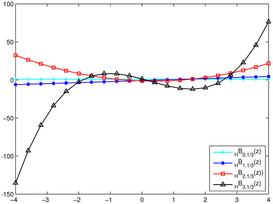
Figure 1. Graph of ${}_{\mathcal{H}}{\mathfrak{B}}_{\kappa ,\mathfrak{q}}(z)$.

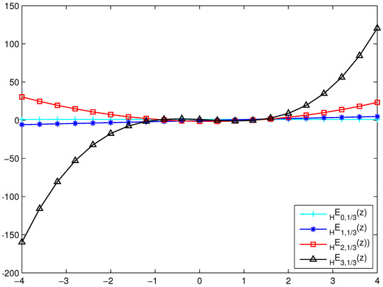
Figure 2. Graph of ${}_{\mathcal{H}}{\mathcal{E}}_{\kappa ,\mathfrak{q}}(z)$.

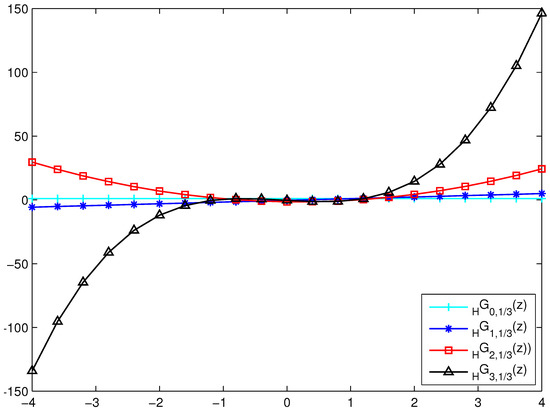
Figure 3. Graph of ${}_{\mathcal{H}}{\mathcal{G}}_{\kappa ,\mathfrak{q}}(z)$.

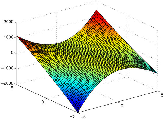
Figure 4. Surface plot of ${}_{\mathcal{H}}{\mathfrak{B}}_{3,\frac{1}{3}}(z_1,z_2)$.

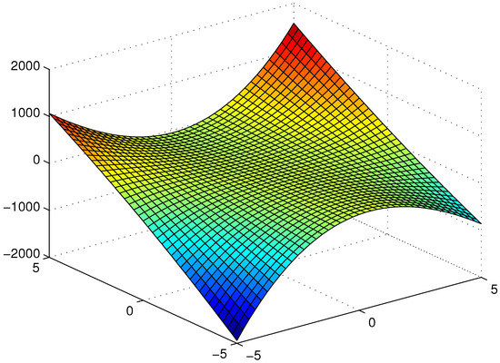
Figure 5. Surface plot of ${}_{\mathcal{H}}{\mathcal{E}}_{3,\frac{1}{3}}(z_1,z_2)$.

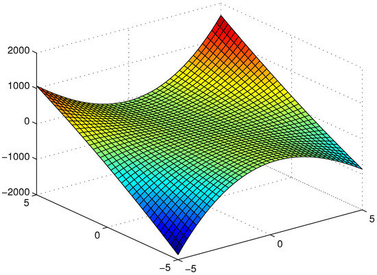
Figure 6. Surface plot of ${}_{\mathcal{H}}{\mathcal{G}}_{3,\frac{1}{3}}(z_1,z_2)$.

6. Further Remarks

It is worth noting that the results derived in the previous sections can be exploited to establish further new relations.

Let us consider the following relation

$${\left[2\right]}_{\mathfrak{q}}^{-\kappa }{D}_{\mathfrak{q},z}^{\kappa }{e}_q(-{\left[2\right]}_{\mathfrak{q}}z\tau )={(-\tau )}^{\kappa }{e}_q(-{\left[2\right]}_{\mathfrak{q}}z\tau ),$$

(96)

which, on replacing $\kappa$ by $2\kappa$ and multiplying both sides of the resultant equation by $\frac{1}{{\left[\kappa \right]}_{\mathfrak{q}}!}$, gives

$$\frac{1}{{\left[\kappa \right]}_{\mathfrak{q}}!}{\left[2\right]}_{\mathfrak{q}}^{-2\kappa }{D}_{\mathfrak{q},z}^{2\kappa }{e}_q(-{\left[2\right]}_{\mathfrak{q}}z\tau )=\frac{1}{{\left[\kappa \right]}_{\mathfrak{q}}!}{(-\tau )}^{2\kappa }{e}_q(-{\left[2\right]}_{\mathfrak{q}}z\tau ).$$

(97)

Now, taking summation on both sides of the above equation and then multiplying both sides of the resultant equation by $\frac{\tau }{e_{\mathfrak{q}}(\tau )-1}$ and using Equation (49), we get

$$\sum _{\kappa =0}^{\infty }{}_{\mathcal{H}}{\mathfrak{B}}_{\kappa ,\mathfrak{q}}(x)\frac{{\tau }^{\kappa }}{{\left[\kappa \right]}_{\mathfrak{q}}!}=\frac{\tau }{e_{\mathfrak{q}}(\tau )-1}\sum _{\kappa =0}^{\infty }\frac{{\left[2\right]}_{\mathfrak{q}}^{-2\kappa }}{{\left[\kappa \right]}_{\mathfrak{q}}!}{D}_{\mathfrak{q},z}^{2\kappa }{e}_q({\left[2\right]}_{\mathfrak{q}}x\tau ),$$

(98)

where $x=-z$.

Similarly, we can obtain the following results:

$$\begin{array}{c}\hfill \sum _{\kappa =0}^{\infty }{}_{\mathcal{H}}{\mathcal{E}}_{\kappa ,\mathfrak{q}}(x)\frac{{\tau }^{\kappa }}{{\left[\kappa \right]}_{\mathfrak{q}}!}=\frac{{\left[2\right]}_{\mathfrak{q}}}{e_{\mathfrak{q}}(\tau )+1}\sum _{\kappa =0}^{\infty }\frac{{\left[2\right]}_{\mathfrak{q}}^{-2\kappa }}{{\left[\kappa \right]}_{\mathfrak{q}}!}{D}_{\mathfrak{q},z}^{2\kappa }{e}_q({\left[2\right]}_{\mathfrak{q}}x\tau ),\end{array}$$

(99)

$$\begin{array}{c}\hfill \sum _{\kappa =0}^{\infty }{}_{\mathcal{H}}{\mathcal{G}}_{\kappa ,\mathfrak{q}}(x)\frac{{\tau }^{\kappa }}{{\left[\kappa \right]}_{\mathfrak{q}}!}=\frac{{\left[2\right]}_{\mathfrak{q}}\tau }{e_{\mathfrak{q}}(\tau )+1}\sum _{\kappa =0}^{\infty }\frac{{\left[2\right]}_{\mathfrak{q}}^{-2\kappa }}{{\left[\kappa \right]}_{\mathfrak{q}}!}{D}_{\mathfrak{q},z}^{2\kappa }{e}_q({\left[2\right]}_{\mathfrak{q}}x\tau ),\end{array}$$

(100)

where $x=-z$.

7. Conclusions

We would like to underline that the $\mathfrak{q}$-series and $\mathfrak{q}$-polynomials have many applications in different fields of mathematics, physics and engineering. In the present article, we demonstrate how a new replacement technique has been adopted to introduce mixed type $\mathfrak{q}$-special polynomials and different method to establish their $\mathfrak{q}$-recurrence relation.

To extend this new and significant approach, the hybrid class of the $\mathfrak{q}$-Sheffer–Appell polynomials and 2D $\mathfrak{q}$-Sheffer–Appell polynomials are introduced by means of series expansion and generating functions. The determinant form related to $\mathfrak{q}$-Sheffer–Appell polynomials are derived, which are important for the computational and applied purposes. This process can be used to establish further a wide variety of formulas and new relations for several other $\mathfrak{q}$-special polynomials.

The $\mathfrak{q}$-difference equation for the two iterated $\mathfrak{q}$-Appell and mixed type $\mathfrak{q}$-Appell polynomials are established in [29,30]. This aspect may be considered in future investigation.

References

- Al-Salam, W.A. q-Appell polynomials. Ann. Mat. Pura Appl. 1967, 4, 31–45. [Google Scholar] [CrossRef]
- Al-Salam, W.A. q-Bernoulli numbers and polynomials. Math. Nachr. 1959, 17, 239–260. [Google Scholar] [CrossRef]
- Araci, S.; Acikgoz, M.; Diagana, T.; Srivastava, H.M. A novel approach for obtaining new identities for the λ extension of q-Euler polynomials arising from the q-umbral calculus. J. Nonlinear Sci. Appl. 2017, 10, 1316–1325. [Google Scholar] [CrossRef]
- Cheon, G.-S.; Jung, J.-H. The q-Sheffer sequences of a new type and associated orthogonal polynomials. Linear Algebra Appl. 2016, 491, 171–186. [Google Scholar] [CrossRef]
- Kim, D.S.; Kim, T.K. q-Bernoulli polynomials and q-umbral calculus. Sci. China Math. 2014, 57, 1867–1874. [Google Scholar] [CrossRef]
- Kim, D.S.; Kim, T.K. Some identities of q-Euler polynomials arising from q-umbral calculus. J. Inequal. Appl. 2014, 2014, 12. [Google Scholar] [CrossRef]
- Kim, T. A note on the q-Genocchi numbers and polynomials. J. Inequal. Appl. 2007, 2007, 071452. [Google Scholar] [CrossRef]
- Kim, D.S.; Kim, T.; Komatsu, T.; Seo, J.-J. An umbral calculus approach to poly-Cauchy polynomials with a q parameter. J. Comput. Anal. Appl. 2015, 18, 762–792. [Google Scholar]
- Kim, D.S.; Kim, T.; Lee, H.Y. p-adic q-integral on Zp associated with Frobenius-type Eulerian polynomials and umbral calculus. Adv. Stud. Contemp. Math. 2013, 23, 243–251. [Google Scholar]
- Andrews, G.E.; Askey, R.; Roy, R. 71th Special Functions of Encyclopedia of Mathematics and Its Applications; Cambridge University Press: Cambridge, UK, 1999. [Google Scholar]
- Aral, A.; Gupta, V.; Agarwal, R.P. Applications of q-Calculus in Operator Theory; Springer: New York, NY, USA, 2013. [Google Scholar]
- Ernst, T. A Comprehensive Treatment of q-Calculus; Springer: Basel, Switzerland; Berlin/Heidelberg, Germany; New York, NY, USA; Dordrecht, The Netherlands; London, UK, 2012. [Google Scholar]
- Appell, P. Sur une classe de polynômes. Ann. Sci. Éc. Norm. Super. 1880, 9, 119–144. [Google Scholar] [CrossRef]
- Thorne, C.J. A property of Appell sets. Am. Math. Mon. 1945, 52, 191–193. [Google Scholar] [CrossRef]
- Sheffer, I.M. Note on Appell polynomials. Bull. Am. Math. Soc. 1945, 51, 739–744. [Google Scholar] [CrossRef]
- Varma, R.S. On Appell polynomials. Proc. Am. Math. Soc. 1951, 2, 593–596. [Google Scholar] [CrossRef]
- Sharma, A.; Chak, A.M. The basic analogue of a class of polynomials. Ann. Probab. Riv. Mat. Univ. Parma 1954, 5, 325–337. [Google Scholar]
- Ernst, T. q-Bernoulli and q-Euler polynomials, an umbral approach. Int. J. Differ. Equ. 2006, 1, 31–80. [Google Scholar]
- Acikgoz, M.; Araci, S.; Duran, U. New extensions of some known special polynomials under the theory of multiple q-calculus. Turkish J. Anal. Number Theory 2015, 3, 128–139. [Google Scholar] [CrossRef]
- Kim, T. q-Generalized Euler numbers and polynomials. Russ. J. Math. Phys. 2006, 13, 293–298. [Google Scholar] [CrossRef]
- Mahmudov, N.I. On a class of q-Bernoulli and q-Euler polynomials. Adv. Differ. Equ. 2013, 4, 108. [Google Scholar] [CrossRef]
- Roman, S.; Rota, G. The umbral calculus. Adv. Math. 1978, 27, 95–188. [Google Scholar] [CrossRef]
- Sheffer, I.M. Some properties of polynomial sets of type zero. Duke Math. J. 1939, 5, 590–622. [Google Scholar] [CrossRef]
- Roman, S. More on the umbral calculus, with emphasis on the q-umbral calculus. J. Math. Anal. Appl. 1985, 107, 222–254. [Google Scholar] [CrossRef]
- Duran, U.; Acikgoz, M.; Esi, A.; Araci, S. A Note on the (p,q)-Hermite Polynomials. Appl. Math. Inf. Sci. 2018, 12, 227–231. [Google Scholar] [CrossRef]
- Hardy, G.H. Divergent Series; American Mathematical Society: Providence, RI, USA, 2000; Volume 334. [Google Scholar]
- Keleshteri, M.E.; Mahmudov, N.I. A study on q-Appell polynomials from determinant point of view. Appl. Math. Comput. 2015, 260, 351–369. [Google Scholar]
- Carlitz, L. q-Bernoulli numbers and polynomials. Duke Math. J. 1948, 15, 987–1000. [Google Scholar] [CrossRef]
- Riyasat, M.; Khan, S.; Nahid, T. q-difference equations for the composite 2D q-Appell polynomials and their applications. Cogent Math. 2017, 4, 1376972. [Google Scholar] [CrossRef]
- Srivastava, H.M.; Khan, S.; Riyasat, M. q-Difference equations for the 2-Iterated q-Appell and mixed type q-Appell Polynomials. Arab. J. Math. 2018, 5, 1–15. [Google Scholar] [CrossRef]
© 2019 by the authors. Licensee MDPI, Basel, Switzerland. This article is an open access article distributed under the terms and conditions of the Creative Commons Attribution (CC BY) license (http://creativecommons.org/licenses/by/4.0/).