Scenario Analysis–Based Decision and Coordination in Supply Chain Management with Production and Transportation Scheduling

Abstract

The production and rail transportation coordinating problem aims to determine a pre-operational timetable for a set of orders. The orders need to be manufactured on a dedicated production line and be delivered to their destination by the pre-planned trains considering traveling routes and time. The connecting trains are an important and even unique chance for orders to reach their final destinations, and earliness and tardiness penalties in the connection and delivery process are closely related to the symmetry and harmony between production procedure decision and train-allocated choice. A scenario analysis method is adopted to reveal the relationships between production collection connecting time (PCCT) and production collection waiting time (PCWT) in the production process. In the delivery process, the relationships between production delivery connecting time (PDCT) and production delivery waiting time (PDWT) are mainly considered. An integrated scheduling coordination model is established to maximize the production connecting time (PCT) and production delivery time (PDT). The GA genetic algorithm is employed to solve this problem. The numerical results show that the coordinated schedule in our method can significantly reduce the number of missed connections when compared with considering delivery timeliness only through a delivery time window. Additionally, it is revealed that the quantitative performances of the delivery timeliness improved by the connecting quality (PCT) are much better than those from the view of the delivery time window (PDT).

1. Introduction

Many studies have involved made-to-order or time-sensitive products (Shen et al. [1], Shu et al. [2], and Federgruen et al. [3]), and finished orders are often delivered to customers immediately or shortly after production. Consequently, production and distribution are very intimately linked and must be scheduled jointly in order to achieve the desired delivery-time performance, at minimum with time-based or cost-based performance measures (Chen [4]). In China, the newest government report noticed that, by 2020, large industrial mining enterprises and newly built logistics parks with an annual volume of over 1.5 million tons will have access to over 80% of dedicated railway lines [5]. This shows that there is a significant benefit in practice in using optimally integrated production–distribution applications (Chen and Variraktarakis [6] and Pundoor and Chen [7]).

The systematic integration of different optimized operation decisions is important for providing better customer service levels at the individual order level. Three types of important challenges are faced in a production–distribution system. One is to coordinate the activities in time and space to determine the production procedure decision and train-allocated choice with the consideration of a line plan and timetable. Rail transportation has a fixed line plan, which specifies the frequency of the line services and their halting patterns (Goossens et al. [8] and Fu et al. [9]). However, air/road transportation uses a point-to-point service mode. Rail transportation is a one-to-many mode, and the service time at each station along the line is defined by a timetable, which specifies the arrival and departure times for each line in the form of a series of trips (Peeters [10]; Zhang and Nie [11]). A train can ship several orders to multiple destinations along the same passage of the railway. This problem is further complicated by the rail timetable coordination between production and rail transportation (Díaz-Madroñero et al. [12] and Sremac et al. [13]). In addition, there is an organizational effort required to measure earliness and tardiness penalties associated with delivery timeliness to restrict the lead times from the production line to the destinations of accessible trips in order to remain within a given time deadline. Compared with applications with fixed delivery departure dates (Li et al. [14,15]; Stecke and Zhao [16]; Wang et al. [17]), the delivery timeliness aspect of the production–rail transportation system is diversifying production procedure decisions and train-allocated choices. Furthermore, the orders must be stowed on the trains within tight time windows imposed by the production procedure decisions and the rail timetable. The importance of tight time windows is illustrated by the scope of urban rail transit (Kang et al. [18]) and by high-speed railway catering services (Wu et al. [19]).

This paper proposes a scheduling model to coordinate production and rail transportation to improve connections and make delivery smoother. The problem was determining the production procedure decision and train-allocated choice with the consideration of the railway timetable. The collection and delivery time analyses are the key details in this paper. The delivery earliness penalty, delivery tardiness penalty and missing connecting train penalty are considered in the optimization objective. The innovations of our study are summarized as follows.

First, a scenario analysis method is used to reveal the relationships between the production collection connecting time (PCCT) and production collection waiting time (PCWT). The time indicators can be employed to distinguish whether one order misses the trains.

Second, a scenario analysis method is used to reveal the relationships between the production delivery connecting time (PDCT) and production delivery waiting time (PDWT). These formulas can be used to estimate the relationship between the order arrival time and delivery time window.

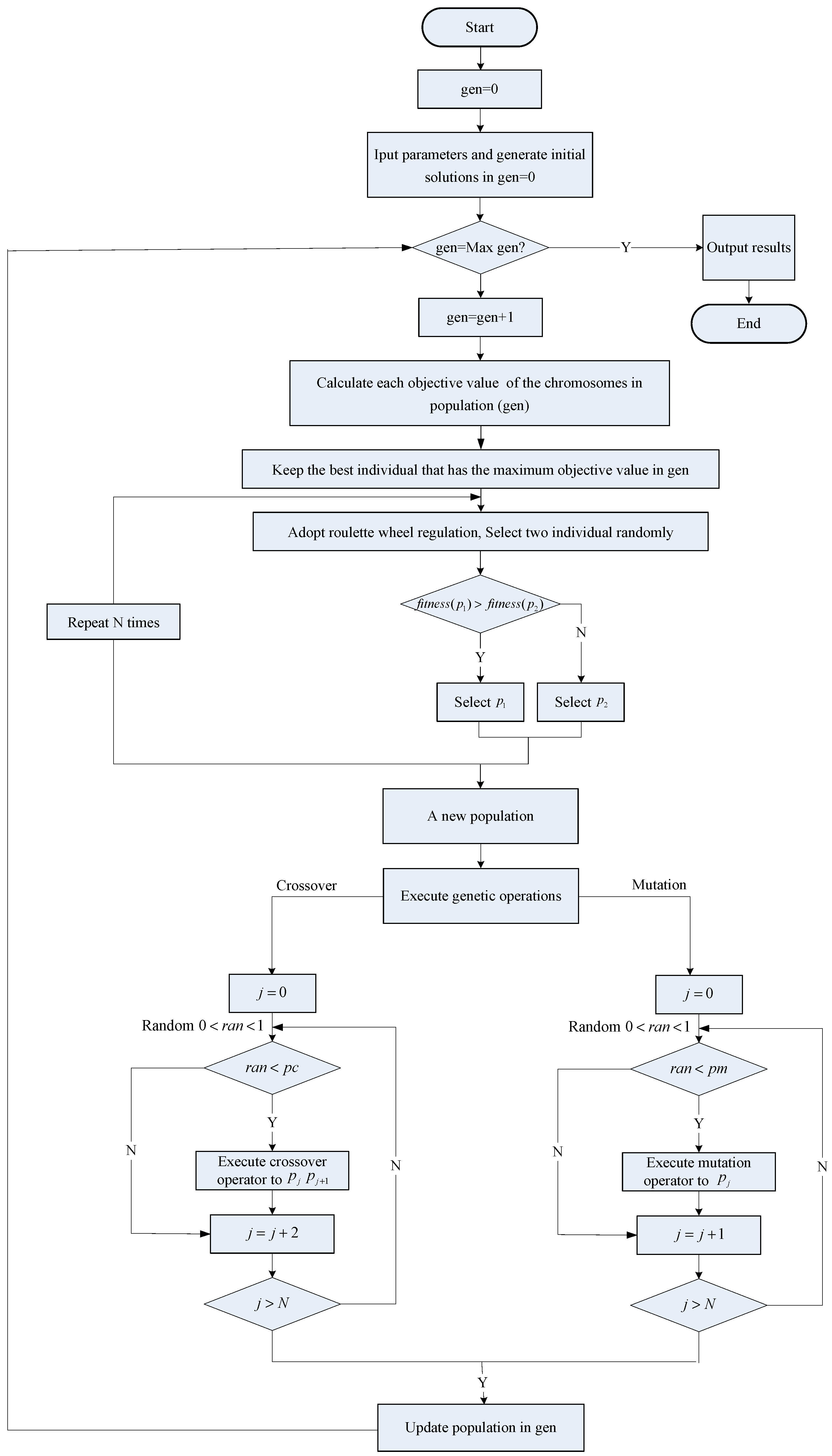
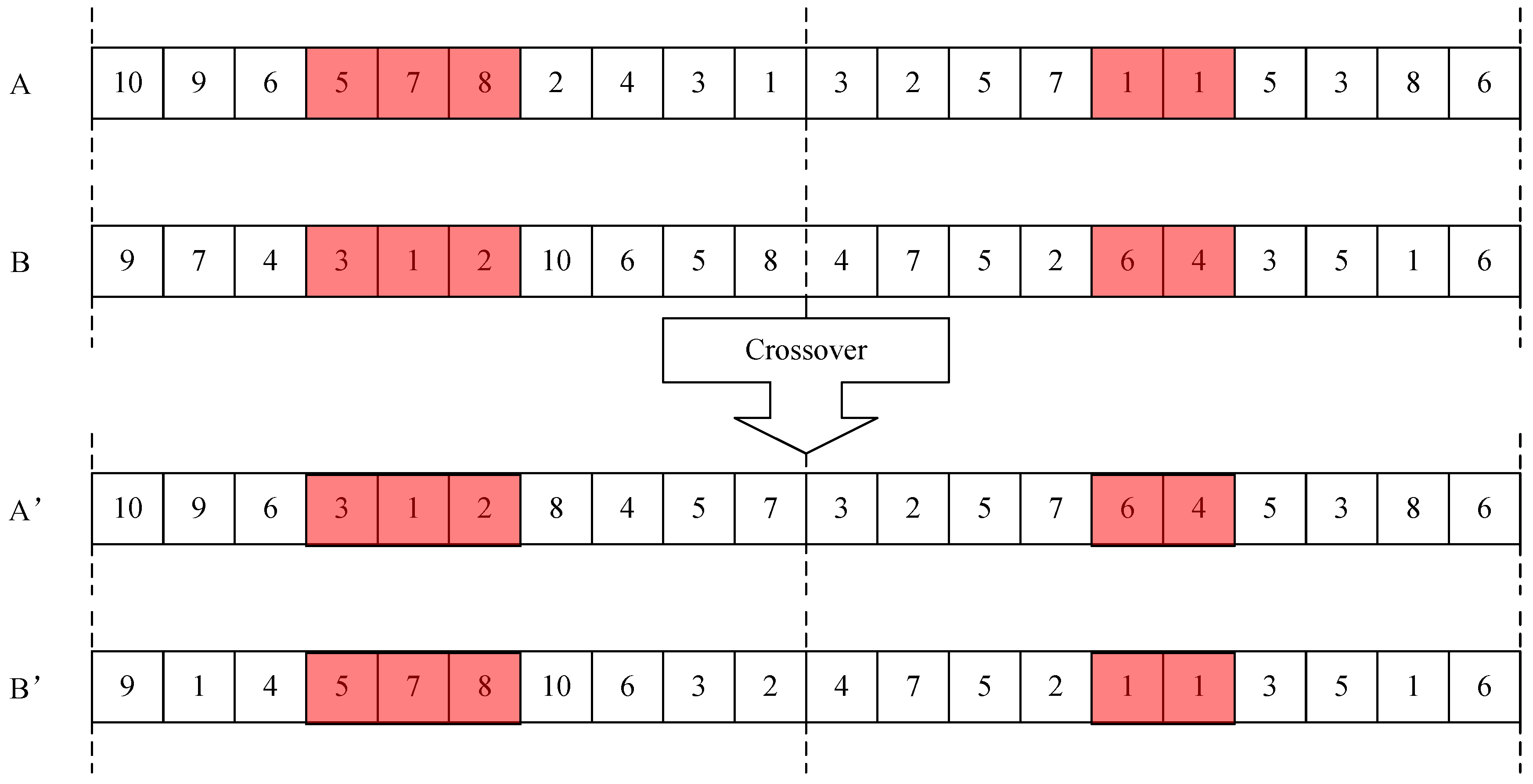
Moreover, a mathematical programming method is developed to solve the problem based on connecting and waiting time. The highlight of our research mainly focused on the time coordination between production and rail transportation. GA is employed to address the model.

2. Literature Review

Research on the integration of scheduling models of production and distribution has been relatively recent and is known as integrated production–distribution planning or scheduling, with studies such as Pundoor et al. [7], Pronsing et al. [20], Zhong et al. [21], Russel et al. [22], Kishimoto et al. [23], and Ma et al. [24]. In many applications including made-to-order or time-sensitive (e.g., perishable, seasonal) products, finished orders are often delivered to customers immediately or shortly after the production. Therefore, the need for integration between supply chain partners is inevitable for these products. Chen [4] summarized the existing integrated production and distribution scheduling models. These models aim to optimize one or a combination of the time-based, cost-based, and revenue-based performance measures [24,25,26,27,28,29,30,31,32] by taking into account relevant fleet size, trucks’ routes, job processing or batching, e.g., Cheng et al. [33], Devapriya et al. [34], and Noroozi et al. [35]. For instance, Hajiaghaei-Keshteli et al. [26] adopt a mathematical modeling method to study the production and transportation system and capacity and cost of rail transportation, which are the highlights of the article. Job delivery and release dates are two importation issues considered in the research by Lu et al. [29]. Ma Y. et al. [24] developed an integrated production–distribution planning model using bi-level programming for supply chain management. Bock [31] addressed time-critical routing on a given path under release dates and deadline restrictions, while the minimization of the total weighted completion time is pursued.

The coordinating and scheduling issues involve both machine scheduling (for order processing) and vehicle scheduling and routing (for order delivery). Delivery in particular is the focus of our article. Trucks are an important transport mode for most orders to reach their destination. A few studies have focused on coordinating the relationship between production and truck scheduling. Chang et al. [25], Chen et al. [4], Zhong et al. [21], Moons [36], Wang et al. [37], Xuan [38], Zhong et al. [39], Seyedhosseini et al. [40], Kang and Lee [41], Ganesan [14], Hajiaghaei-Keshteli et al. [26], Zandieh [42], and Delavar et al. [43] proposed mathematical models to optimize the production and road and air transportation coordinating problem. For instance, an integrated production and distribution scheduling problem is considered by Devapriya et al. [34], and in this research, the trucks’ routes and the fleet size are the important decisions. Moons et al. [36] developed a study on a production and distribution system, and decisions on vehicle routing received considerable attention. Sawik [44] discussed the production and distribution scheduling problem in supply chains with regional and local disruption risks. Azadian et al. [45] researched the order contract producing problem from a manager’s perspective and proposed an integrated scheduling model on the coordination of production and transportation planning. It is not difficult to see that this class of problems define delivery shipments that are allowed to visit multiple customers. Hence, it is necessary to find a route (i.e., sequence of customers to visit) for each delivery shipment. Such a routing problem alone is already intractable in many cases because it contains the strongly NP-hard traveling salesman problem (TSP) as a special case (Chen [4]).

Although there are many works on the study of production–distribution issues as mentioned above, the coordination between production and rail transportation in an operational time dimension is one of the less focused-upon aspects. Several similar versions of this problem, termed the production road/air transportation problem, have been studied in Moons et al. [36] and Li et al. [46]. Compared with the airline transportation problem, air transportation is also apparently affected by the flight plan and aircrafts used (Pemberton [47]; Liang et al. [48]; Ho et al. [49]), but the loading required by each flight is usually satisfied at its origin port. Nevertheless, in the rail transportation problem, a train can either be loaded at a trip’s origin or at its other passing station. At any rate, the difficulty degree of the airline transportation problem is reduced on this point alone. Hence, the distribution system design integrated the knowledge of path selecting, and the time window caused by the rail timetable makes our issue more novel and interesting. In addition to this, according to the schedule, the connecting trains provide a very important as well as unique opportunity for orders to reach their final destinations in time (Kang et al. [18] and Wu et al. [19]). Producers and customers tend to complain more when orders miss the connecting trains to their destinations. These characteristics lead to some difficulties to apply the off-the-shelf technologies in a production–distribution system. To the best of our knowledge, few studies have been conducted to investigate these topics in the context of railway timetables.

In conclusion, our method not only takes relevant accessibility into account, but also takes delivery timeliness as a time window constraint into account. Of course, this is more common in other articles. However, more importantly, not only the delivery timeliness (customer service levels at the individual order level) is guaranteed by the tight delivery time window, but also a comprehensive formula is introduced to measure delivery timeliness or customer service levels at the individual order level. The comprehensive formula can be used to distinguish between the last feasible connecting train and the non-last ones and be used to judge whether the feasible connecting trains will be missed. Meanwhile, the comprehensive formula is employed to improve the connecting relationship between the production line and trains. This comprehensive formula is summarized from the scenario analysis introduced in our research.

3. Integrated Scheduling Coordination Model

3.1. Basic Assumptions

To facilitate the model formulation, we consider the following assumptions throughout this paper:

Assumption 1.

The transfer operating time ($t_{sl{l}^{\prime }}^{Tra}$) and delivery operating time ($t_{e{l}^{\prime }}^{Tra}$) are known and fixed for all orders. Although not all orders have the same quantity, $t_{sl{l}^{\prime }}^{Tra}$ and $t_{e{l}^{\prime }}^{Tra}$ are assumed constant for simplification.

Assumption 2.

It can be assumed that the production line and related rail station are at the same geographical position. The same assumption applies for the order destination and the related train.

Assumption 3.

We regard the production line as a single machine, and no free time is allowed.

3.2. Production Connecting Connection Time (PCCT) and Waiting Time (PCWT)

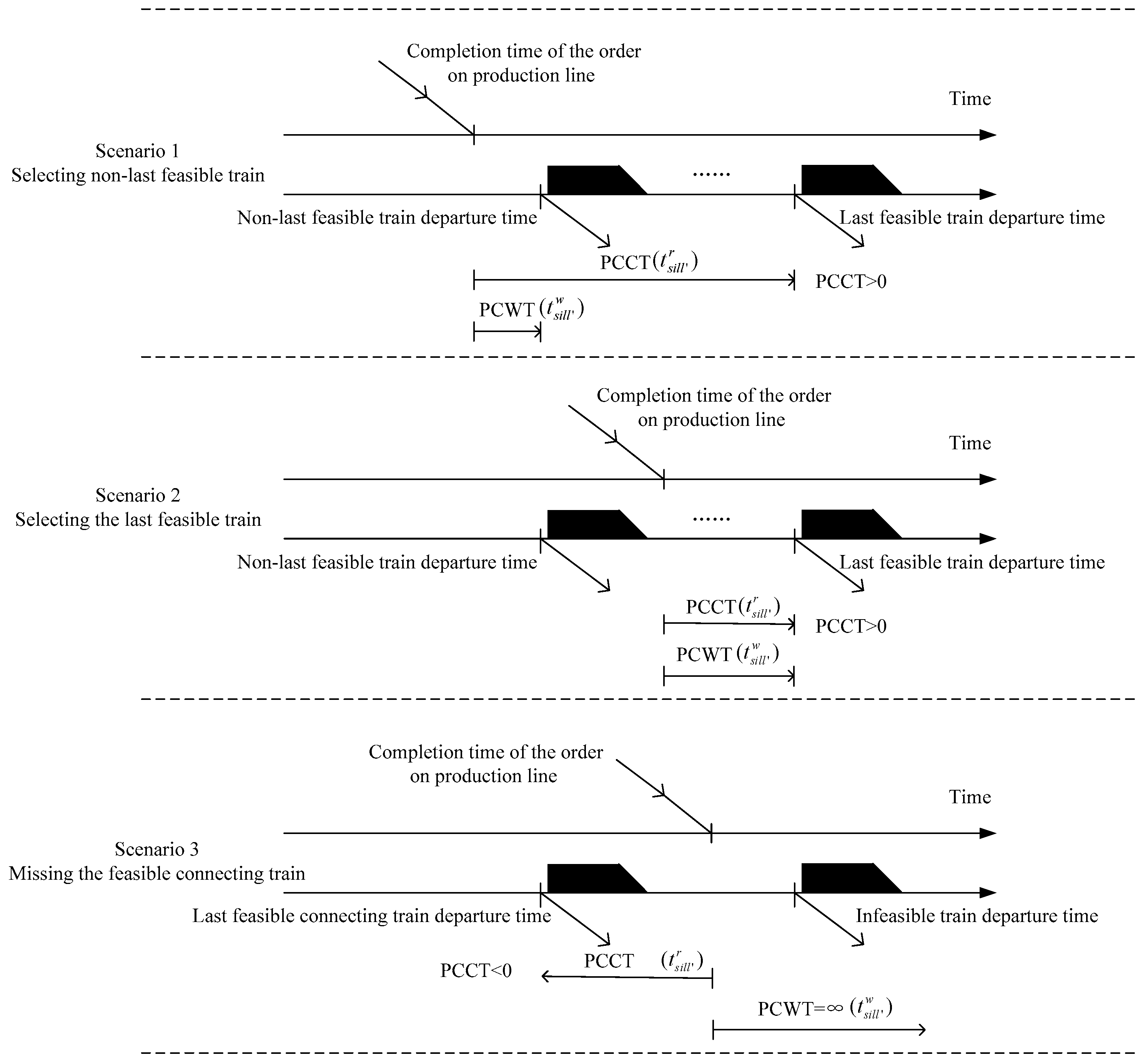
The PCCT could be evaluated by $t_{sil{l}^{\prime }}^r=t_{s{l}^{\prime }}^D-t_{sil}^A-t_{sl{l}^{\prime }}^{Tra}$, where $t_{s{l}^{\prime }}^D$ represents the departure time of the last feasible connecting train $l^{\prime }$ from station $s$; $t_{sil}^A$ represents the completion time of the order $i$ at station $s$ on production line $l$, and it is determined by its production sequence; $t_{sl{l}^{\prime }}^{Tra}$ represents the operating time from $l$ to $l^{\prime }$ at station $s$. If $t_{sil{l}^{\prime }}^r\ge 0$, the order can connect to the feasible train successfully. However, the order fails to connect when $t_{sil{l}^{\prime }}^r<0$.

Regarding the PCWT, $t_{sil{l}^{\prime }}^w$, is defined as the waiting time when the order transfers from the production line $l$ to the selected connecting train $l^{\prime }$. If orders fail to transfer to a feasible connecting train, PCWT is defined as a sufficiently large value.

As mentioned above, $t_{sil{l}^{\prime }}^r$ and $t_{sil{l}^{\prime }}^w$ can be calculated by Equation (1), where $M$ represents a sufficiently large positive value.

$$\{\begin{array}{l}{t}_{sil{l}^{\prime }}^r=t_{s{l}^{\prime }}^D-t_{sil}^A-t_{sl{l}^{\prime }}^{Tra}\\ t_{sil{l}^{\prime }}^w=x_{il{l}^{\prime }}\cdot t_{s{l}^{\prime }}^{D^{\prime }}-t_{sil}^A-t_{sl{l}^{\prime }}^{Tra}+(1-x_{il{l}^{\prime }})\cdot M\end{array}$$

(1)

Three different relationships based on the orders’ completion times and train departure times are shown in Figure 1. The timeline above represents the completion time of the order at station $s$ on production line $l$, while the below timeline captures the departure times of connecting trains at station $s$ on line $l^{\prime }$.

(1)

As scenario 1 shows, if PCCT > PCWT, orders will choose the non-last feasible connecting train instead of the last feasible one, in which $t_{sil{l}^{\prime }}^r-t_{sil{l}^{\prime }}^w>0$.

(2)

As scenario 2 shows, if PCCT = PCWT, orders will choose the last feasible connecting train; that is, $t_{sil{l}^{\prime }}^r-t_{sil{l}^{\prime }}^w=0$.

(3)

However, if no feasible train can be chosen, as shown in scenario 3, PCCT is defined as a negative value, and PCWT is a sufficiently large positive value; that is, PCCT < PCWT. Orders will fail to connect; that is, $t_{sil{l}^{\prime }}^r-t_{sil{l}^{\prime }}^w<0$. We let $t_{sil{l}^{\prime }}^r-t_{sil{l}^{\prime }}^w=-\theta$ to simplify the numerical calculation. $\theta$ is defined as the penalty value of missing the feasible connecting train.

From the above, we propose a composite indicator as production connection time (PCT, $t_{sil{l}^{\prime }}^h$) in Equation (2). Orders can connect successfully between $l$ and $l^{\prime }$ when $t_{sil{l}^{\prime }}^h\ge 0$, otherwise, $t_{sil{l}^{\prime }}^h<0$.

$$t_{sil{l}^{\prime }}^h=\{\begin{array}{l}{t}_{sil{l}^{\prime }}^r-t_{sil{l}^{\prime }}^w>0,\mathrm{when}{t}_{s{l}^{\prime }}^D-(t_{sil}^A+t_{sl{l}^{\prime }}^{Tra})>t_{s{l}^{\prime }}^D-t_{s{l}^{\prime }}^{D^{\prime }}\\ t_{sil{l}^{\prime }}^r-t_{sil{l}^{\prime }}^w=0,\mathrm{when}0\le t_{s{l}^{\prime }}^D-(t_{sil}^A+t_{sl{l}^{\prime }}^{Tra})\le t_{s{l}^{\prime }}^D-t_{s{l}^{\prime }}^{D^{\prime }}\\ t_{sil{l}^{\prime }}^r-t_{sil{l}^{\prime }}^w=-\theta ,\mathrm{when}{t}_{s{l}^{\prime }}^D-(t_{sil}^A+t_{sl{l}^{\prime }}^{Tra})<0\end{array}$$

(2)

3.3. Production Delivery Connection Time (PDCT) and Waiting Time (PDWT)

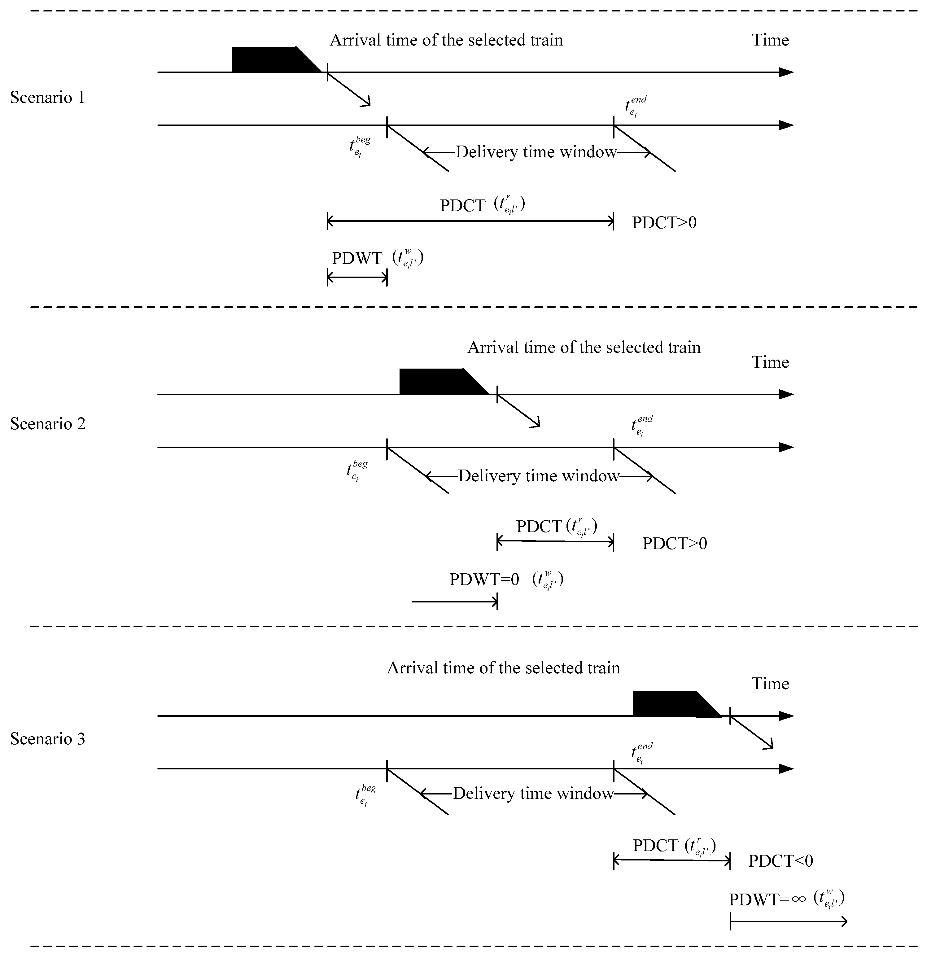
At each delivery destination $e_i$, the PDCT is decided by the selected train arrival time and the end time of the time window for the order $i$ because the delivery time from line $l^{\prime }$ to the customers is constant, as assumed. Thus, PDCT is calculated by $t_{e_i{l}^{\prime }}^r=t_{e_i}^{end}-x_{il{l}^{\prime }}\cdot t_{e_i{l}^{\prime }}^A-t_{e{l}^{\prime }}^{Tra}-(1-x_{il{l}^{\prime }})\cdot M$, where M is a sufficiently large positive value, $t_{e_i{l}^{\prime }}^A$ represents the arrival time of the selected train $l^{\prime }$ to its delivery destination; $t_{e_i}^{end}$ represents the end delivery time for the order $i$; and $t_{e{l}^{\prime }}^{Tra}$ represents the order delivery operating time from line $l^{\prime }$ to customers. Orders can deliver successfully between rail transportation and customers when $t_{e_i{l}^{\prime }}^r\ge 0$. However, orders fail to transfer when $t_{e_i{l}^{\prime }}^r<0$.

The PDWT, $t_{e_i{l}^{\prime }}^w$, is the waiting time for the order until the delivery service allowed by the time window. If the train arrival time is beyond the due time, orders may not successfully be delivered, and PDWT approaches an infinite positive number. Therefore, $t_{e_i{l}^{\prime }}^r$ and $t_{e_i{l}^{\prime }}^w$ can be calculated by Equation (3).

$$\{\begin{array}{l}{t}_{e_i{l}^{\prime }}^r=t_{e_i}^{end}-x_{il{l}^{\prime }}\cdot t_{e_i{l}^{\prime }}^A-t_{e{l}^{\prime }}^{Tra}-(1-x_{il{l}^{\prime }})\cdot M\\ t_{e_i{l}^{\prime }}^w=\max \{t_{e_i}^{beg}-x_{il{l}^{\prime }}\cdot t_{e_i{l}^{\prime }}^A-t_{e{l}^{\prime }}^{Tra}+(1-x_{il{l}^{\prime }})\cdot M,0\}+M\cdot \max \{x_{il{l}^{\prime }}\cdot t_{e_i{l}^{\prime }}^A-t_{e_i}^{end}-(1-x_{il{l}^{\prime }})\cdot M,0\}\end{array}$$

(3)

Three different relationships based on the selected train arrival time and delivery time window are shown in Figure 2. The timeline above shows the selected train arrival time to the order’s destination, while the arrows below capture the delivery time window of the order.

(1)

If PDCT − PDWT > 0 and PDWT > 0 (scenario 1), orders will be delivered early to the destination, in which case $t_{e_i{l}^{\prime }}^r-t_{e_i{l}^{\prime }}^w>0$. We let $t_{e_i{l}^{\prime }}^r-t_{e_i{l}^{\prime }}^w=-\alpha$, and this means the penalty value of delivering early.

(2)

If PDCT − PDWT > 0 and PDWT = 0 (scenario 2), orders can be delivered as soon as the connecting train arrives, in which $t_{e_i{l}^{\prime }}^r-t_{e_i{l}^{\prime }}^w>0$. We let $t_{e_i{l}^{\prime }}^r-t_{e_i{l}^{\prime }}^w=\mu$ to facilitate the numerical calculation.

(3)

However, if PDCT − PDWT < 0, and PDCT < 0 (scenario 3), orders will fail to deliver, and $t_{e_i{l}^{\prime }}^r-t_{e_i{l}^{\prime }}^w<0$. In this case, $t_{e_i{l}^{\prime }}^w$ is a sufficiently large positive value, and $t_{e_i{l}^{\prime }}^r$ is a negative value, implying $t_{e_i{l}^{\prime }}^r-t_{e_i{l}^{\prime }}^w=-M$. We let $t_{e_i{l}^{\prime }}^r-t_{e_i{l}^{\prime }}^w=-\delta$, and the meaning of $\delta$ is the penalty value of delivering late. Let $\left|\delta \right|\gg \left|\alpha \right|$.

Here, we define a production delivery time (PDT,$t_{e_i{l}^{\prime }}^d$) in formula (4).

$$t_{e_i{l}^{\prime }}^d=\{\begin{array}{l}{t}_{e_i{l}^{\prime }}^r-t_{e_i{l}^{\prime }}^w=-\alpha ,\mathrm{when}{x}_{il{l}^{\prime }}\cdot t_{e_i{l}^{\prime }}^A+t_{e{l}^{\prime }}^{Tra}<t_{e_i}^{beg}\\ t_{e_i{l}^{\prime }}^r-t_{e_i{l}^{\prime }}^w=\mu ,\mathrm{when}{t}_{e_i}^{beg}<x_{il{l}^{\prime }}\cdot t_{e_i{l}^{\prime }}^A+t_{e{l}^{\prime }}^{Tra}<t_{e_i}^{end}\\ t_{e_i{l}^{\prime }}^r-t_{e_i{l}^{\prime }}^w=-\delta ,\mathrm{when}{x}_{il{l}^{\prime }}\cdot t_{e_i{l}^{\prime }}^A+t_{e{l}^{\prime }}^{Tra}>t_{e_i}^{end}\end{array}$$

(4)

3.4. Model Formulation

In the integrated scheduling coordination model, the objective function contains two aspects. On one hand, the model is intended to maximize PCCT and PDCT. If PCCT > 0, orders can choose one feasible connecting train successfully. Otherwise, orders fail to connect. Similarly, if PDCT > 0, orders can be delivered successfully. Otherwise, orders fail to deliver. However, some orders may fail to transfer and deliver because of production procedure decisions. On the other hand, the model expects to minimize PCWT and PDWT. From Equations (2) and (4), two integrative variables are defined here (PCT and PDT). Thus, the objective function is to maximize $t_{sil{l}^{\prime }}^h$ and $t_{ei{l}^{\prime }}^d$ to increase successful connections /deliveries and reduce waiting time.

$$\mathrm{MAX}T={\displaystyle \sum _{s\in S}{\displaystyle \sum _{i\in I}{\displaystyle \sum _{l\in L}{\displaystyle \sum _{l^{\prime }\in L^{\prime }}{t}_{sil{l}^{\prime }}^h}}}}+{\displaystyle \sum _{e_i\in E}{\displaystyle \sum _{l^{\prime }\in L^{\prime }}{t}_{e_i{l}^{\prime }}^d}}$$

(5)

(1) For any order $i\in I$ in the production line $l\in L$, Equation (6) is given to determine the completion time of the order $i$ at station $s$ on production line $l$.

$$t_{sil}^A={\displaystyle \sum _{j=1}^k(u_{ij}\cdot (p_i\cdot Q_i+{\displaystyle \sum _{j^{\prime }=1}^{j-1}{\displaystyle \sum _{i^{\prime }=1}^k{u}_{i^{\prime }{j}^{\prime }}\cdot p_{i^{\prime }}\cdot Q_{i^{\prime }}}}))}$$

(6)

$$u_{ij}\in \{0,1\}\forall ij$$

(7)

$${\displaystyle \sum _{i=1}^k{u}_{ij}}=1\forall j$$

(8)

$${\displaystyle \sum _{j=1}^k{u}_{ij}}=1\forall i$$

(9)

(2) Some equipment requirements that set limits on the capacity for connecting trains should be satisfied.

$${\displaystyle \sum _{l\in L}{\displaystyle \sum _{i\in I}{x}_{il{l}^{\prime }}\cdot Q_i}}\le Ca{p}_{l^{\prime }}\forall l^{\prime }$$

(10)

(3) From Equations (2) and (4), we define $t_{sil{l}^{\prime }}^h$ and $t_{e_i{l}^{\prime }}^d$.

$$t_{sil{l}^{\prime }}^h=\{\begin{array}{l}{t}_{sil{l}^{\prime }}^r-t_{sil{l}^{\prime }}^w>0,\mathrm{when}{t}_{s{l}^{\prime }}^D-(t_{sil}^A+t_{sl{l}^{\prime }}^{Tra})>t_{s{l}^{\prime }}^D-t_{s{l}^{\prime }}^{D^{\prime }}\\ t_{sil{l}^{\prime }}^r-t_{sil{l}^{\prime }}^w=0,\mathrm{when}0\le t_{s{l}^{\prime }}^D-(t_{sil}^A+t_{sl{l}^{\prime }}^{Tra})\le t_{s{l}^{\prime }}^D-t_{s{l}^{\prime }}^{D^{\prime }}\\ t_{sil{l}^{\prime }}^r-t_{sil{l}^{\prime }}^w=-\theta ,\mathrm{when}{t}_{s{l}^{\prime }}^D-(t_{sil}^A+t_{sl{l}^{\prime }}^{Tra})<0\end{array}$$

(11)

$$t_{e_i{l}^{\prime }}^d=\{\begin{array}{l}{t}_{e_i{l}^{\prime }}^r-t_{e_i{l}^{\prime }}^w=-\alpha ,\mathrm{when}{x}_{il{l}^{\prime }}\cdot t_{e_i{l}^{\prime }}^A+t_{e{l}^{\prime }}^{Tra}<t_{e_i}^{beg}\\ t_{e_i{l}^{\prime }}^r-t_{e_i{l}^{\prime }}^w=\mu ,\mathrm{when}{t}_{e_i}^{beg}<x_{il{l}^{\prime }}\cdot t_{e_i{l}^{\prime }}^A+t_{e{l}^{\prime }}^{Tra}<t_{e_i}^{end}\\ t_{e_i{l}^{\prime }}^r-t_{e_i{l}^{\prime }}^w=-\delta ,\mathrm{when}{x}_{il{l}^{\prime }}\cdot t_{e_i{l}^{\prime }}^A+t_{e{l}^{\prime }}^{Tra}>t_{e_i}^{end}\end{array}$$

(12)

4. Solution Algorithm and Numerical Experiment

Scheduling production associated with rail transportation is quite complex because it involves a complex combination of relationships. Additionally, the problem is subject to a number of considerations such as successful connections, just-in-time delivery and technical equipment constraints. The integrated problems such as production–distribution and the location-routing problem are NP-hard problems and thus are difficult to solve using exact algorithms (Perl and Daskin [50]). Heuristic approaches generally become more viable alternatives as the problem size increases (Nagy and Salhi [51]). Therefore, it is important in the view of management to develop an effective algorithm for this problem. Intelligent optimization algorithms are usually employed to deal with complex combinations and various types of problems. For example, the genetic algorithm (GA), simulated annealing (SA) algorithm [49], cross entropy method [19], and branch and bound (B&B) method are commonly used, and GA is especially widely used.

4.1. Genetic Algorithm

The production procedure decisions and train-allocated choices are considered to be genes for a chromosome. One chromosome represents a solution, and real number encoding is utilized. The chromosome is arranged as the vector ($u_{i1}$, …, $u_{kj}$; $x_{1l{l}^{\prime }}$, …, $x_{kl{l}^{\prime }}$), where $k$ is the number of orders. Figure 3 is a sample network containing one production line, ten orders and eight train lines. The starting point of all trains is assumed to be the “production facility”. A sample chromosome of the network is shown in Figure 4, which is divided into two sections, and the two sections are the order position and train selection, respectively. For instance, the first ten numbers in Figure 4 represent a stochastic ordering of the orders in the production line. The circled element of the chromosome indicates that the No. 8 order is arranged at position one. Meanwhile, the triangle element represents the No. 8 order being allocated to the No. 3 train after production processing. In this paper, the initial solution is created randomly.

Figure 5 shows the flow of the GA process, and it includes two key steps, which are crossover and mutation. We adopt the replacing method in the crossover operation; i.e., the gene’s values at the same position of the two chromosomes are exchanged (see Figure 6). The mutation operator helps GA to escape from local convergence. The mutation operator just rearranges the structure of the chromosome and makes the population more diverse. The last basic issue in the GA is the algorithm termination criterion. In this paper, if iterations reach the preset number, the GA will terminate its computational process [52].

4.2. Numerical Test

The scheduling model and GA are tested on the sample network shown in Figure 3 which contains one production line, six railway stations associated with the orders destination and eight rail service lines with different running paths. The starting point of all trains is the “production facility”. The rail timetable is listed in

Table 1. Timetable of the sample network.

Station Line	Departure Time	1	2	3	4	5	6
1	1	3.5	-	5	-	7.5	-
2	1.5	-	4.5	-	-	-	-
3	2	3	-	4.5	-	-	6
4	2.5	4.5	-	5.5	-	8	-
5	3	5	-	-	6.5	-	-
6	3.5	4.5	-	6.5		7.5	-
7	4	-	5.5	-	-	-	-
8	4.5	5.5	-	-	7	-	-

. The second column indicates the train departure time, and the others represent the train arrival time to each station.

The nonzero elements in the third to the eighth column in Table 1 describe the track of the rail lines. The order can be allocated to one or multiple trains which reach its destination. For example, we can allocate the order 1 to train 1, 3, 4, or 6 to reach destination 3.

4.2.1. Sample Network Test

We test the model and GA algorithm on a personal computer with Intel Core i5, 2.60 GHz CPU and 4GB RAM. We set the population size to be 100, crossover fraction to be 0.9, mutation rate to be 0.1 and the GA’s maximum number of iterations to be 200. Let $\theta =100$, $\alpha =10$, $\mu =10$ and $\delta =100$. The GA can solve the model in a very short time, and the detailed results are shown in

Table 2. Timetable of the sample network.

Quality/Processing Time	0.3/1	0.4/1	0.2/1	0.2/1	0.1/1	0.1/3	0.1/5	0.1/3	0.4/2	0.2/4
Delivery time window	[1,10]	[1,6]	[1,6]	[1,8]	[1,7]	[1,10]	[1,8]	[1,5]	[1,9]	[1,4]
Production scheduling and train allocated	10	4	2	8	6	7	3	1	9	5
1	√
2		√	√
3				√						√
4					√
5						√	√
6								√
7
8									√
$t_{sil{l}^{\prime }}^r$	2.7	2.8	2.6	0.1	1.5	2.2	1.7	0.4	0.6	−0.2
$t_{sil{l}^{\prime }}^w$	0.2	0.3	0.1	0.1	0.5	0.7	0.2	0.4	0.6	∞
$t_{e_i{l}^{\prime }}^r$	1.5	0.5	0.5	1.0	−0.2	2.5	0.5	−2.5	2.5	0
$t_{e_i{l}^{\prime }}^w$	0	0	0	0	0	0	0	0	0	0

. The PCWT, $t_{sil{l}^{\prime }}^w$, is the key indicator of production success connection. The PCWT of order 5 is a sufficiently large number, so order 5 is unsuccessful at catching train 3. Meanwhile, PDWT > 0 is the only condition of success delivery. Form Table 2, we can see that order 1 and 6 fail to deliver (here, we do not consider the effect of the unsuccessful connection for order 5.). The number of successful deliveries is 8, achieving 90% successful transfer in the sample system.

4.2.2. Performance of GA and Convergence Test

In this section, we adopt the Simulated Annealing (SA), Tabu Srearch (TS), and Particle Swarm Optimization (PSO) algorithms to solve the numerical network again, and compare the performances of them with GA. The results of all algorithms are similar, but the CPU times are different. As shown in

Table 3. Results of coordination by different methods.

Method	Successful Connections	Successful Deliveries	Objective Function	CPU Time (s)
GA	9	8	−207.5	15.6
SA	9	8	−206.5	74.7
TS	9	8	−208.0	16.7
PSO	9	8	−206.5	27.2

, it costs GA 15.6 s to get an optimal solution, and TS takes an approximately equal time. However, the SA approach takes 75 s. Figure 7 compares the solution time of each algorithm, where the x-axis describes the CPU time and the y-axis is the corresponding objective function. In conclusion, the GA is better in both quality and solution time.

The objective value is contributed by PCCT, PCWT, PDCT, and PDWT. By optimizing the objective, the coordinated schedule makes the order connection and delivery in the system among the production line, rail transportation and destination consumers smooth and reasonable. Figure 8 shows the GA convergence curve, and we can obtain the optimal solution with GA at nearly 10 iterations. The circle represents the best objective value at each iteration.

4.2.3. Comparisons of Different Objectives

To verify the proposed model (Max PCT+PDT), the objective functions of Max PCT and Max PDT are tested to compare them with the optimization results of our model. The test is performed under the same conditions and with the same data.

Table 4. Results of different objectives.

Objective	Successful Connections	Successful Deliveries	Total Waiting Time in Both Connection and Delivery Process
Max PCT	9	7	402
Max PDT	4	8	806.6
Max (PCT+PDT)	9	8	302

lists the details of the results. Note that when $t_{sil{l}^{\prime }}^w$ and $t_{e_i{l}^{\prime }}^w$ approach $\infty$, $t_{sil{l}^{\prime }}^w$ and $t_{e_i{l}^{\prime }}^w$ are set to be 100 in this experiment to compare the waiting time easily. There are nine successful connections and seven successful deliveries for Max PCT and the total waiting time is 402. However, for Max PDT, the number of successful connections is reduced to 9. The total waiting time is reduced to 806.6. Compared with Max PCT and Max PDT, Max (PCT+PDT) can obtain an obvious improvement in the number of successful deliveries (8) and successful connections (9).

4.2.4. Analysis of Penalty Parameters and GA Parameters

In addition, the effects of $\theta$, $\alpha$, $\mu$, and $\delta$ on the scheduling coordination are discussed. Taking $\theta$ as an example, the values of $\theta$ are tested from 10 to 100 with 10 intervals, shown as the first column in

Table 5. Analysis of the effects of the penalty parameter.

Penalty θ	Successful Connections	Successful Deliveries	PCCT	PCWT for Successful Connections	PCT for Missing Connections	PDCT	PDWT for Successful Deliveries	PDT for Missing Deliveries	Objective Function
10	9	8	15.5	2.2	−10	6.5	0	−200	−116.5
20	9	8	15.3	2.0	−20	6.5	0	−200	−126.5
30	9	8	15.3	2.0	−30	6.5	0	−200	−136.5
40	9	8	15.5	2.2	−40	6.5	0	−200	−146.5
50	9	8	15.3	2.0	−50	6.5	0	−200	−156.5
60	9	8	15.5	2.2	−60	6.5	0	−200	−166.5
70	9	8	15.5	2.2	−70	6.5	0	−200	−176.5
80	9	8	15.4	2.6	−80	6.5	0	−200	−186.5
90	9	8	15.4	2.6	−90	6.5	0	−200	−197
100	9	8	12.8	3.0	−100	4	0	−200	−206.5

. The model always draws almost the same conclusion that the number of successful deliveries is 8 and the number of successful transfers is 9 in the sample system. This phenomenon can be explained as follows. The connection relation of production and rail transportation is definite when the train timetable is shown as in Table 1. According to equation (2), just one order is in the case of $t_{sil{l}^{\prime }}^r-t_{sil{l}^{\prime }}^w=-\theta$ in the optimal schedule. Thus, the schedule is identical even if the value of $\theta$ is changed from 10 to 100.

Two key GA parameters connected with the problem scale are analyzed in this section. It reveals that the optimal results can achieve a certain improvement when we set a bigger population size ($N$) and a larger generation ($K$). As shown in

Table 6. Different objective values corresponding to varying GA parameters.

N\K	0	50	100	200	300	400	500
0	0	0	0	0	0	0	0
50	0	−207.5	−207.5	−207.5	−207.5	−207.0	−207.0
100	0	−207.5	−207.5	−207.5	−207.5	−207.0	−207.0
200	0	−207.5	−207.5	−207.5	−207.5	−207.0	−207.0
300	0	−207.5	−207.5	−207.5	−207.5	−207.0	−207.0
400	0	−207.5	−207.5	−207.5	−207.0	−207.0	−207.0
500	0	−207.5	−207.5	−207.5	−207.0	−206.5	−206.5

, different problem scales are solved with different combinations with $N$ and $K$. When $N=0$ or $K=0$, GA cannot work.

5. Conclusions

There are many studies on the study of production–distribution issues, but few works focus on the coordinating timetable of rail transportation with the production sequence. This paper focuses on procedure decisions and train-allocated choices with the consideration of railway timetables.

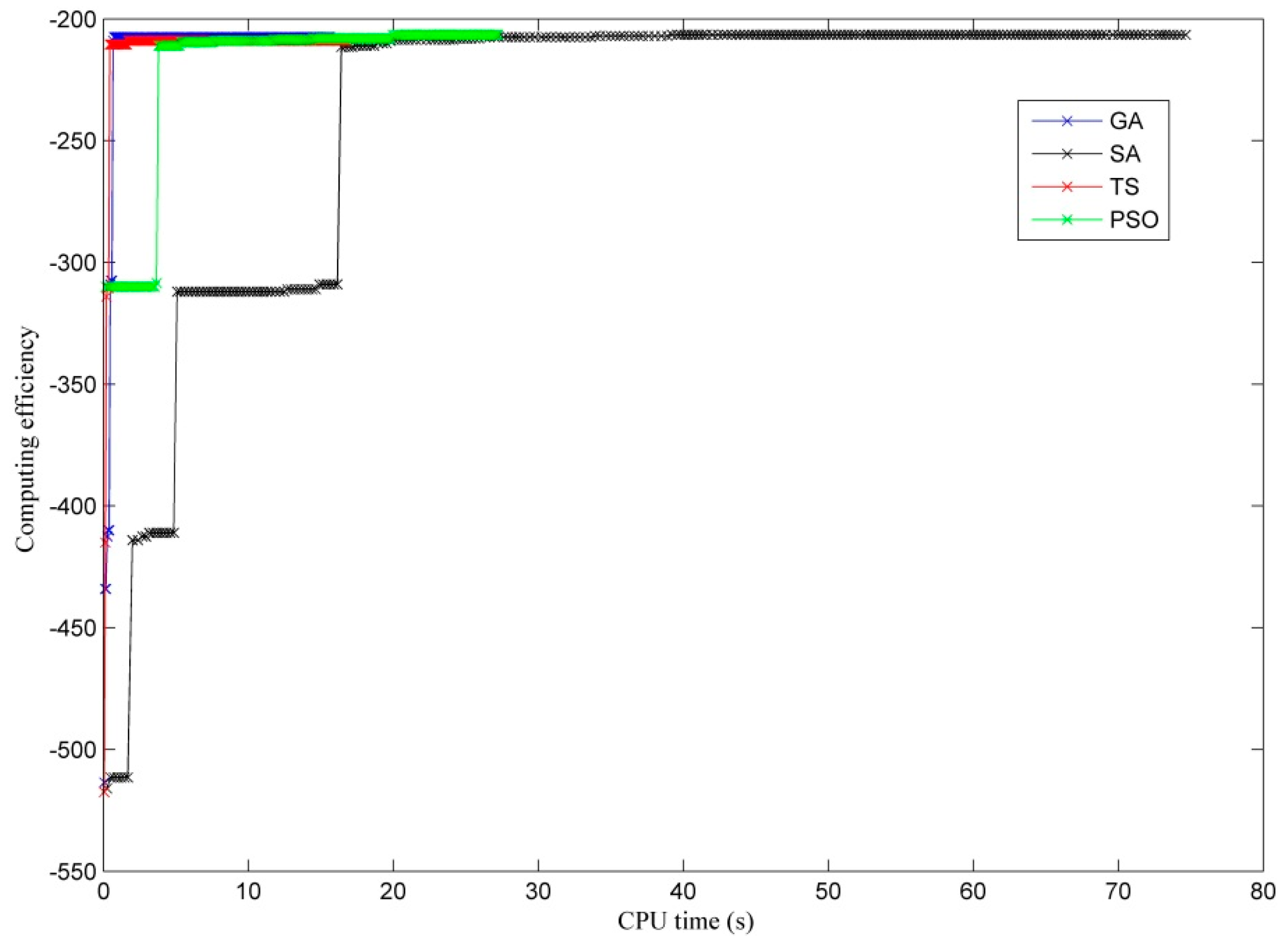
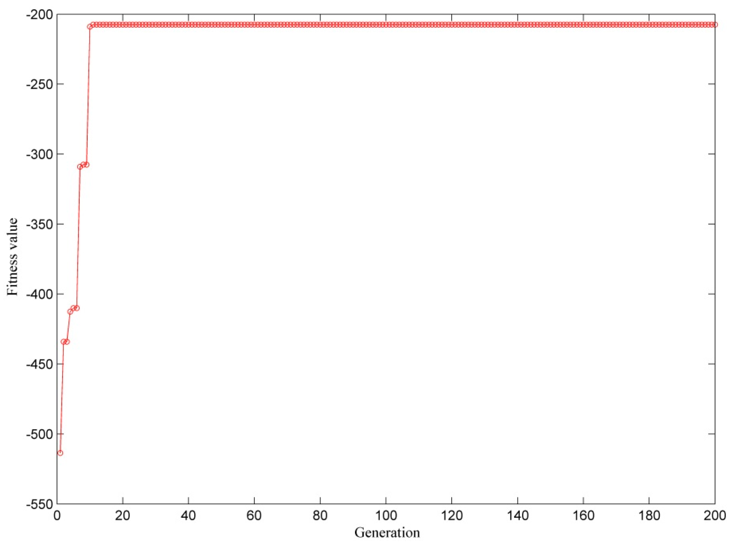
A scenario analysis method is used to reveal the relationships between PCCT and PCWT in the production process and the relationships between PDCT and PDWT in the delivery process. An integrated scheduling coordination model is established to maximize the production connecting time (PCT) and production delivery time (PDT). The model and GA are applicable and easy to implement. The results indicate that the more successful connections and deliveries in the network that are achieved are attributed to our model.

Our research can be furthered in several areas. First, considering both ordinary trains and charter trains in the problem makes the problem more interesting, because the timetable for charter trains can be personalized to meet order demand. Moreover, actual trains in service may miss their scheduling because of unexpected incidents, so it is worth discussing how a dynamic rescheduling strategy which aims to eliminate the negative effects could be made.

References

1. Shen, M.Z.J.; Coullard, C.; Daskin, M.S. A joint location-inventory model. Transport. Sci. 2003, 37, 40–55. [Google Scholar] [CrossRef]
2. Shu, J.; Teo, C.; Shen, Z.M. Stochastic transportation-inventory network design problem. Oper. Res. 2005, 53, 48–60. [Google Scholar] [CrossRef]
3. Federgruen, A.; Prastacos, G.; Zipkin, P.H. An allocation and distribution model for perishable products. Oper. Res. 1986, 34, 75–82. [Google Scholar] [CrossRef]
4. Chen, Z.L. Integrated production and outbound distribution scheduling: Review and extensions. Oper. Res. 2010, 58, 130–148. [Google Scholar] [CrossRef]
5. Three-year action plan for promoting transport structural adjustment (2018–2020). MOT. 2018.
6. Chen, Z.-L.; Vairaktarakis, G.L. Integrated scheduling of production and distribution operations. Manag. Sci. 2005, 51, 614–628. [Google Scholar] [CrossRef]
7. Pundoor, G.; Chen, Z.-L. Scheduling a production-distribution system to optimize the tradeoff between delivery tardiness and total distribution cost. Nav. Res. Logist. 2005, 52, 571–589. [Google Scholar] [CrossRef]
8. Goossens, J.W.; Hoesel, S.V.; Kroon, L. On solving multi-type railway line planning problems. Eur. J. Oper. Res. 2006, 168, 403–424. [Google Scholar] [CrossRef] [Green Version]
9. Fu, H.; Nie, L.; Meng, L.; Sperry, B.R.; He, Z. A hierarchical line planning approach for a large-scale high speed rail network: The China case. Transport. Res. Part A 2015, 75, 61–83. [Google Scholar] [CrossRef]
10. Peeters, L. Cyclic Railway Timetable Optimization. Ph.D. Thesis, Erasmus University Rotterdam, Rotterdam, The Netherlands, 2003. [Google Scholar]
11. Zhang, X.; Nie, L. Integrating capacity analysis with high-speed railway timetabling: A minimum cycle time calculation model with flexible overtaking constraints and intelligent enumeration. Transport. Res. Part C 2016, 68, 509–531. [Google Scholar] [CrossRef]
12. Díaz-Madroñero, M.; Peidro, D.; Mula, J. A review of tactical optimization models for integrated production and transport routing planning decisions. Comput. Ind. Eng. 2015, 88, 518–535. [Google Scholar] [CrossRef]
13. Sremac, S.; Stević, Ž.; Pamučar, D.; Arsić, M.; Matić, B. Evaluation of a Third-Party Logistics (3PL) Provider Using a Rough SWARA–WASPAS Model Based on a New Rough Dombi Aggregator. Symmetry 2018, 10, 305. [Google Scholar] [CrossRef]
14. Li, K.P.; Ganesan, V.K.; Sivakumar, A.I. Synchronized scheduling of assembly and multi-destination air-transportation in a consumer electronics supply chain. Int. J. Prod. Res. 2005, 43, 2671–2685. [Google Scholar] [CrossRef]
15. Li, K.P.; Ganesan, V.K.; Sivakumar, A.I. Scheduling of single stage assembly with air transportation in a consumer electronic supply chain. Comput. Ind. Eng. 2006, 51, 264–278. [Google Scholar] [CrossRef]
16. Stecke, K.E.; Zhao, X. Production and transportation integration for a make-to-order manufacturing company with a commit-to-delivery business mode. Manuf. Serv. Oper. Manag. 2007, 9, 206–224. [Google Scholar] [CrossRef]
17. Wang, H.; Lee, C.-Y. Production and transport logistics scheduling with two transport mode choices. Nav. Res. Logist. 2005, 52, 796–809. [Google Scholar] [CrossRef]
18. Kang, L.J.; Wu, J.J.; Sun, H.J.; Zhu, X.N.; Wang, B. A practical model for last train rescheduling with train delay in urban railway transit networks. Omega 2015, 50, 29–42. [Google Scholar] [CrossRef]
19. Wu, X.; Nie, L.; Xu, M. Designing an integrated distribution system for catering services for high-speed railways: A three-echelon location routing model with tight time windows and time deadlines. Transport. Res. C 2017, 74, 212–244. [Google Scholar] [CrossRef]
20. Pornsing, C.; Tharawetcharak, P.; Jomthong, P.; Tonglim, T. Particle swarm optimization for integrated production-distribution scheduling problem. In Proceedings of the 2017 3rd International Conference on Control, Automation and Robotics (ICCAR), Nagoya, Japan, 24–26 April 2017. [Google Scholar]
21. Zhong, X.; Jiang, D. Integrated Scheduling of Production and Distribution with Release Dates and Capacitated Deliveries. Math. Probl. Eng. 2016, 2016, 9315197. [Google Scholar] [CrossRef]
22. Russel, R.; Chiang, W.C.; Zepeda, D. Integrating multi-product production and distribution in newspaper logistics. Comput. Oper. Res. 2008, 35, 1576–1588. [Google Scholar] [CrossRef]
23. Kishimoto, T.; Fugo, K.; Kiyokawa, T. Integrated production and intermodal transportation planning in large scale production–distribution-networks. Transport. Res. E 2013, 60, 62–78. [Google Scholar]
24. Ma, Y.F.; Yan, F.; Kang, K.; Wei, X.G. A novel integrated production-distribution planning model with conflict and coordination in a supply chain network. Knowl.-Based Syst. 2016, 105, 119–133. [Google Scholar] [CrossRef]
25. Chang, Y.C.; Lee, C.Y. Machine scheduling with job delivery coordination. Eur. J. Oper. Res. 2004, 158, 470–487. [Google Scholar] [CrossRef]
26. Hajiaghaei-Keshteli, M.; Aminnayeri, M.; Ghomi, S.M.T.F. Integrated scheduling of production and rail transportation. Comput. Ind. Eng. 2014, 74, 240–256. [Google Scholar] [CrossRef]
27. Lee, C.Y.; Chen, Z.L. Machine scheduling with transportation considerations. J. Sched. 2001, 4, 3–24. [Google Scholar] [CrossRef] [Green Version]
28. Soukhal, A.; Oulamara, A.; Martineau, P. Complexity of flow shop scheduling problems with transportation constraints. Eur. J. Oper. Res. 2005, 161, 32–41. [Google Scholar] [CrossRef] [Green Version]
29. Lu, L.; Yuan, J.; Zhang, L. Single machine scheduling with release dates and job delivery to minimize the makespan. Theor. Comput. Sci. 2008, 393, 102–108. [Google Scholar] [CrossRef] [Green Version]
30. Tang, L.; Gong, H. The coordination of transportation and batching scheduling. Appl. Math. Model. 2009, 33, 3854–3862. [Google Scholar] [CrossRef]
31. Bock, S. Finding optimal tour schedules on transportation paths under extended time window constraints. J. Sched. 2016, 19, 1–20. [Google Scholar] [CrossRef]
32. Liu, S.; Lin, B.; Wu, J.; Zhao, Y. Modeling the Service Network Design Problem in Railway Express Shipment Delivery. Symmetry 2018, 10, 391. [Google Scholar] [CrossRef]
33. Cheng, B.Y.; Leung, J.Y.T.; Li, K. Integrated scheduling of production and distribution to minimize total cost using an improved ant colony optimization method. Comput. Ind. Eng. 2015, 83, 217–225. [Google Scholar] [CrossRef]
34. Devapriya, P.; Ferrell, W.; Geismar, N. Integrated Production and Distribution Scheduling with a Perishable Product. Eur. J. Oper. Res. 2017, 259, 906–916. [Google Scholar] [CrossRef]
35. Noroozi, A.; Mazdeh, M.M.; Heydari, M.; Rasti-Barzoki, M. Coordinating order acceptance and integrated production-distribution scheduling with batch delivery considering Third Party Logistics distribution. J. Manuf. Syst. 2018, 46, 29–45. [Google Scholar] [CrossRef]
36. Moons, S.; Ramaekers, K.; An, C.; Arda, Y. Integrating production scheduling and vehicle routing decisions at the operational decision level: A review and discussion. Comput. Ind. Eng. 2016, 104, 224–245. [Google Scholar] [CrossRef]
37. Wang, X.; Cheng, T.C.E. Machine scheduling with an availability constraint and job delivery coordination. Nav. Res. Logist. 2007, 54, 11–20. [Google Scholar] [CrossRef]
38. Xuan, H. Hybrid Flowshop Scheduling with Finite Transportation Capacity. Appl. Mech. Mater. 2011, 65, 574–578. [Google Scholar] [CrossRef] [Green Version]
39. Zhong, W.; Dósa, G.; Tan, Z. On the machine scheduling problem with job delivery coordination. Eur. J. Oper. Res. 2015, 182, 1057–1072. [Google Scholar] [CrossRef]
40. Seyedhosseini, S.M.; Ghoreyshi, S.M. An Integrated Model for Production and Distribution Planning of Perishable Products with Inventory and Routing Considerations. Math. Probl. Eng. 2014, 2014, 475606. [Google Scholar] [CrossRef]
41. Kang, H.-Y.; Lee, A.H.I. An Enhanced Approach for the Multiple Vehicle Routing Problem with Heterogeneous Vehicles and a Soft Time Window. Symmetry 2018, 10, 650. [Google Scholar] [CrossRef]
42. Zandieh, M.; Molla-Alizadeh-Zavardehi, S. Synchronizing Production and Air Transportation Scheduling Using Mathematical Programming Models; Elsevier Science Publishers: Amsterdam, The Netherlands, 2009. [Google Scholar]
43. Delavar, M.R.; Hajiaghaei-Keshteli, M.; Molla-Alizadeh-Zavardehi, S. Genetic algorithms for coordinated scheduling of production and air transportation. Expert Syst. Appl. 2010, 37, 8255–8266. [Google Scholar] [CrossRef]
44. Sawik, T. Stochastic versus Deterministic Approach to Coordinated Supply Chain Scheduling. Math. Probl. Eng. 2017, 2017, 3460721. [Google Scholar] [CrossRef]
45. Azadian, F.; Murat, A.; Chinnam, R.B. Integrated production and logistics planning: Contract manufacturing and choice of air/surface transportation. Eur. J. Oper. Res. 2015, 247, 113–123. [Google Scholar] [CrossRef]
46. Li, S.; Li, M. Integrated Production and Distribution Scheduling Problems Related to Fixed Delivery Departure Dates and Weights of Late Orders. Sci. World J. 2015, 2015, 804968. [Google Scholar] [CrossRef] [PubMed]
47. Pemberton, R.G. A lotus 1-2-3 model for airline level of operations planning. Comput. Ind. Eng. 1986, 11, 330–334. [Google Scholar] [CrossRef]
48. Liang, W.; Li, Y. Research on optimization of flight scheduling problem based on the combination of ant colony optimization and genetic algorithm. In Proceedings of the 2014 IEEE 5th International Conference on Software Engineering and Service Science, Beijing, China, 27–29 June 2014; pp. 296–299. [Google Scholar]
49. Ho, S.C.; Leung, J.M.Y. Solving a manpower scheduling problem for airline catering using metaheuristics. Eur. J. Oper. Res. 2010, 202, 903–921. [Google Scholar] [CrossRef]
50. Perl, J.; Daskin, M. A warehouse location-routing problem. Transport. Res. Part. B 1985, 19, 381–396. [Google Scholar] [CrossRef]
51. Nagy, G.; Salhi, S. Location-routing: Issues, models and methods. Eur. J. Oper. Res. 2007, 177, 649–672. [Google Scholar] [CrossRef] [Green Version]
52. Shafahi, Y.; Khani, A. A practical model for transfer optimization in a transit network: Model formulations and solutions. Transport. Res. A 2010, 44, 377–389. [Google Scholar] [CrossRef]
Figure 1. Effects of production connecting time (PCT) on production collection. PCCT: production collection connecting time; PCWT: production collection waiting time.
Symmetry 11 00160 g001
Figure 2. Effects of production delivery time (PDT) on production delivery. PDCT: production delivery connection time; PDWT: production delivery waiting time.
Symmetry 11 00160 g002
Figure 3. Illustration of the sample network.
Symmetry 11 00160 g003
Figure 4. A chromosome for the sample network.
Symmetry 11 00160 g004
Figure 5. Flow of the genetic algorithm (GA) process.
Symmetry 11 00160 g005
Figure 6. Crossover operation.
Symmetry 11 00160 g006
Figure 7. The time required by each algorithm to reach its best solution.
Symmetry 11 00160 g007
Figure 8. GA convergence curve for the sample network.
Symmetry 11 00160 g008