1. Introduction
Verhulst is credited with formulating the ordinary differential equation (ODE)
and coining the name logistic [
1,
2]. Later investigators proposed variations on the Verhulst equation (e.g., difference logistic equation), sometimes continuing to refer to these as logistic models. The first application of ODE (1) was connected with population problems, and more generally, problems in ecology. If the Verhulst model is used for describing change in population size
N over time
t, then in Equation (1)
is the Malthusian parameter (rate of maximum population growth) and
is the carrying capacity (i.e., the maximum sustainable population). Equation (1) is widely used in problems of ecology, economics, chemistry, medicine, pharmacology, epidemiology, etc. [
3,
4,
5,
6,
7,
8]. As a rule, this model is oversimplified for quantitative estimations, but reflects the key qualitative features of processes under consideration.
Equation (1) can be reduced to the form
where
The Cauchy problem (Equations (2) and (3)) has the exact solution
The discrete logistic equation can be written as follows
where parameter
characterizes the rate of reproduction (growth) of the population;
, parameter
defines the time between consecutive measurements.
The nonlinear difference Equation (5) exhibits period doubling to chaos [
5,
6].
We will analyze a slightly different discrete logistic equation
Difference Equation (6) is obtained from ODE (2) using a forward difference scheme for the derivative with the step of discretization h.
Ordinary difference equation (O
E) (6) is close enough in behavior to solutions to the equation [
4,
5]
OE (7) is close enough in behavior to solutions to Equation (6) for .
Initial condition for O
Es (5), (6) or (7) is
The discrete Cauchy problems (5) and (8), (6) and (8) or (7) and (8) for sufficiently large values of the parameter
describe the complex, chaotic behavior of the system [
3,
4,
5,
6,
7,
8]. For O
E (6), as it is shown in [
3] for
the solution starts to oscillate periodically around the value
. This solution is stable as long as
. For
the process comes to steady periodic oscillations with a period of four.
It can be mentioned that the chaotic threshold for O
E (7) is 2.6824 [
4,
5].
After describing the objects of our research, we proceed to the formulation of its goals. Both continuous and discrete logistic equations have been extensively investigated. The results of these studies are described in a large number of research and review books and papers [
4,
5,
6,
7,
8,
9]. Our study focuses on the discretization and continualization of nonlinear ODE and O
E, while the logistic equations serve only as convenient and simple examples.
First problem: is it possible to discretize ODE (6) in such a way that the resulting O
E has only regular solutions? This practically important issue has been studied quite well [
10,
11,
12,
13], and we, in fact, only briefly present the known results.
On the other hand, many researchers point that discrete logistic models are more adequate to the essence of the physical, economic or biological processes precisely because they have chaotic regimes [
3]. In this regard, our second problem is: can such a continualization of the original O
E be proposed that the resulting ODE has a chaotic solution? The practical value of these equations can be considered controversial, but the construction of such continualization procedure is interesting.
It is difficult to expect that standard continualization, based on the Taylor series, will provide the desired result. It remains to be hoped for the techniques based on the use of Padé approximants [
14].
The paper is organized as follows: In
Section 2 we propose discretization of Verhulst ODE without chaotic behavior. Continualization of the discrete Verhulst equation using Padé approximants is described in
Section 3. Then, in
Section 4 we display and discuss some results of numerical integrations. Finally, in
Section 5 some conclusions are presented.
3. Continualization with Padé Approximants
Let us try to construct a continuous model (i.e., ODE), describing the chaotic behavior like original O
E. As it is mentioned in [
9], for generating chaotic behavior nonlinear ODE must have dimension
To construct a logistic-like ODE with chaotic behavior, additional modifications were introduced—piecewise constant argument, delay, and fractional derivative [
15,
16,
17,
18]. We use continualization based on Maclaurin expansion and Padé approximants.
For continualization of O
E (6) let us introduce the continuous coordinate
scaled in such a way that
. Suppose
slightly changing function we use Maclaurin expansion
The third order equation thus obtained
describes completely deterministic trajectories.
Let us consider fluctuations around the second equilibrium position,
. Using changing of variables
one obtains
The initial condition for this difference equation can be written as follows
Suppose
slightly changing function we use Maclaurin expansion
The fifth order ODE can be written as follows
Equation (16) describes deterministic trajectories.
Transform the differential operator in square brackets of Equation (16) into the diagonal Padé approximation [2,2], we obtain:
Then
and after routine transformations one obtains:
Point after (17) must be omitted
Let us formulate initial conditions for the third order ODE (17). From the initial condition for original difference Equation (15) one obtains
Additional initial conditions for Equation (17) we choose in the following form:
Point after (19) must be omitted
Initial value problem (Equations (17) and (19)) can be transformed by going to “dimensionless time”
, to the following form:
4. Numerical Results
Numerical integration of Cauchy problem (Equations (20) and (21)) is carried out using the Adams–Bashforth–Moulton method (a predictor-corrector method), where is found by first applying the Adams–Bashforth method (the predictor), then using the Adams–Bashforth–Moulton method (the corrector).
The calculations were performed in the Maple 18 computing environment. The graphs below are depicted in the original variable .
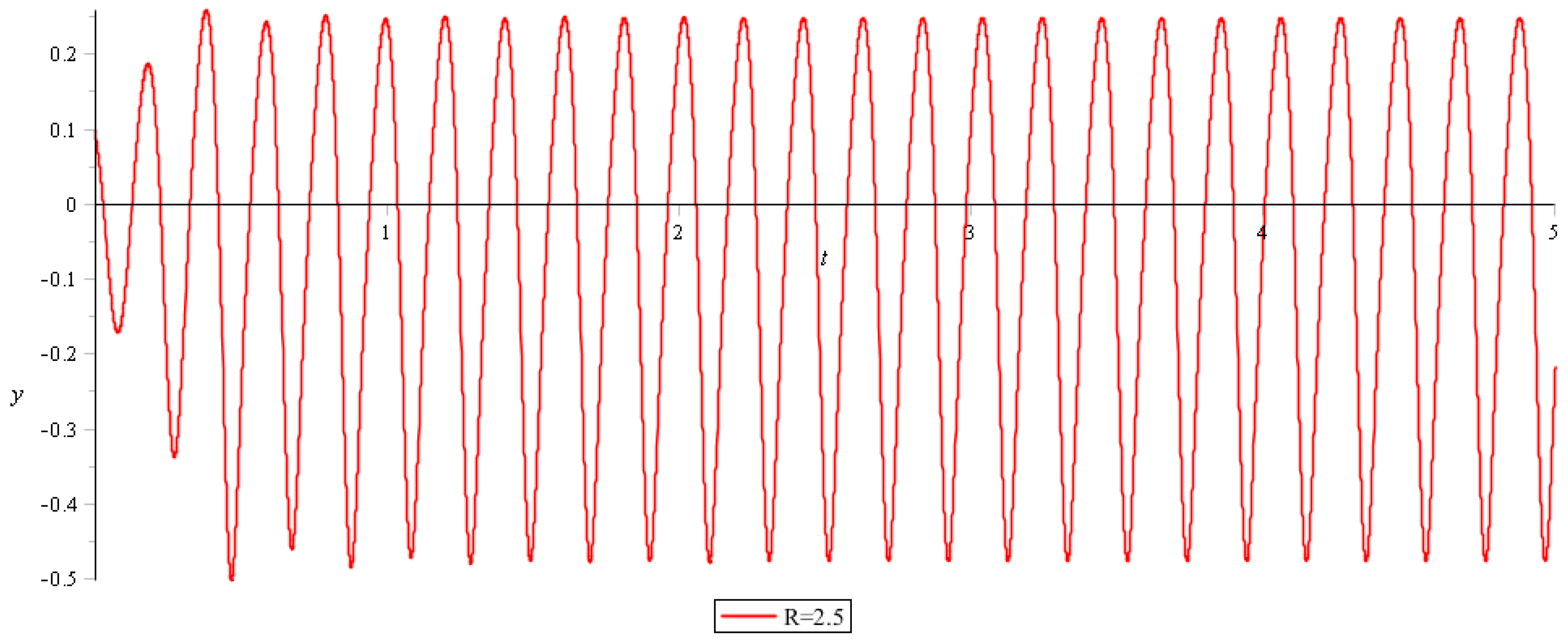
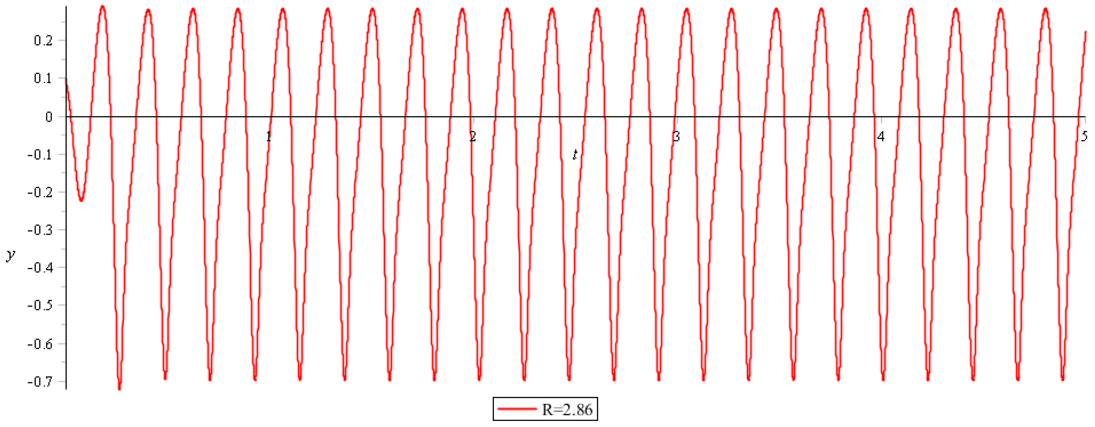
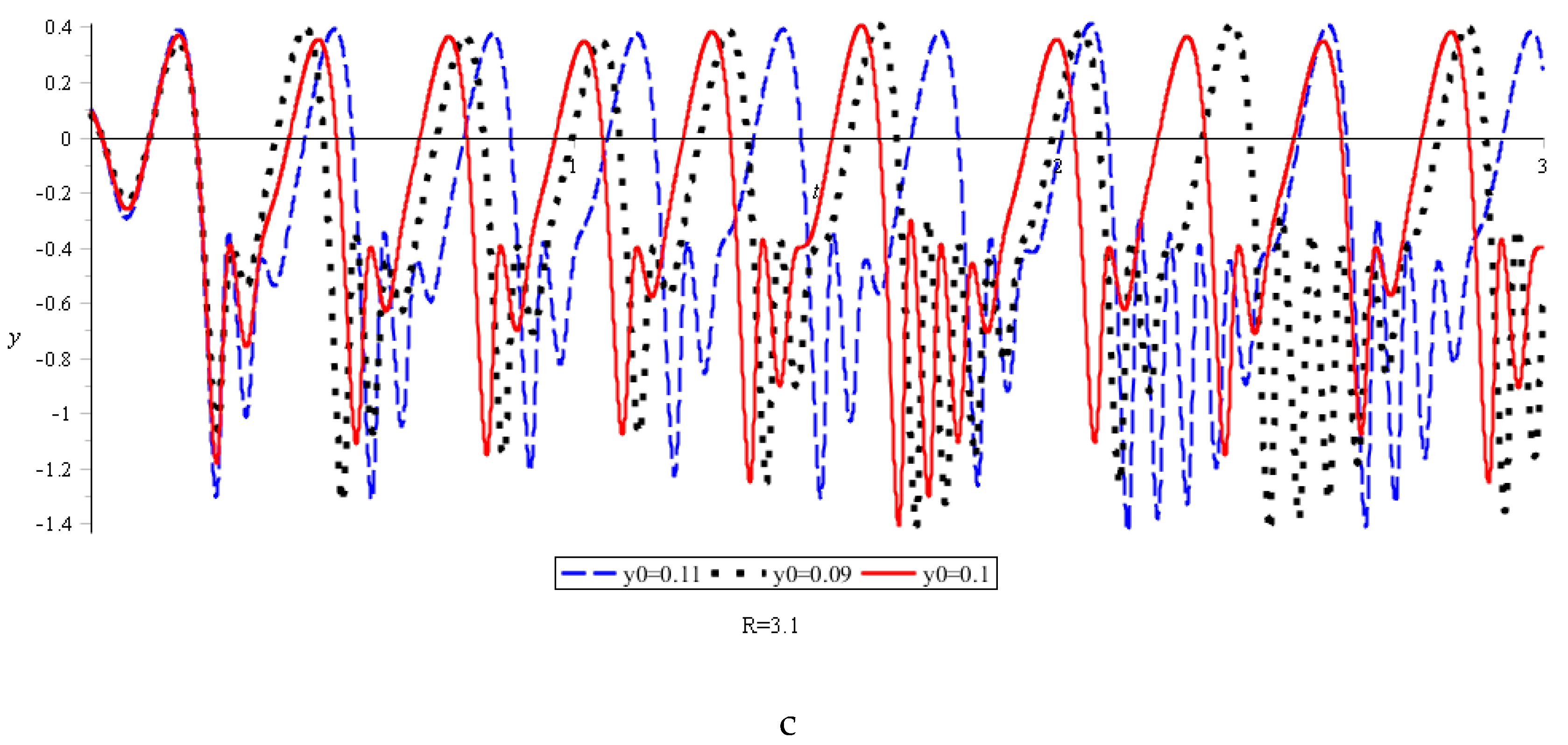
The presented numerical results can be divided into three groups: describing periodic oscillations, periodic oscillations with subharmonics, and the chaotic oscillations. For
one obtains periodic oscillations (
Figure 1,
Figure 2 and
Figure 3).
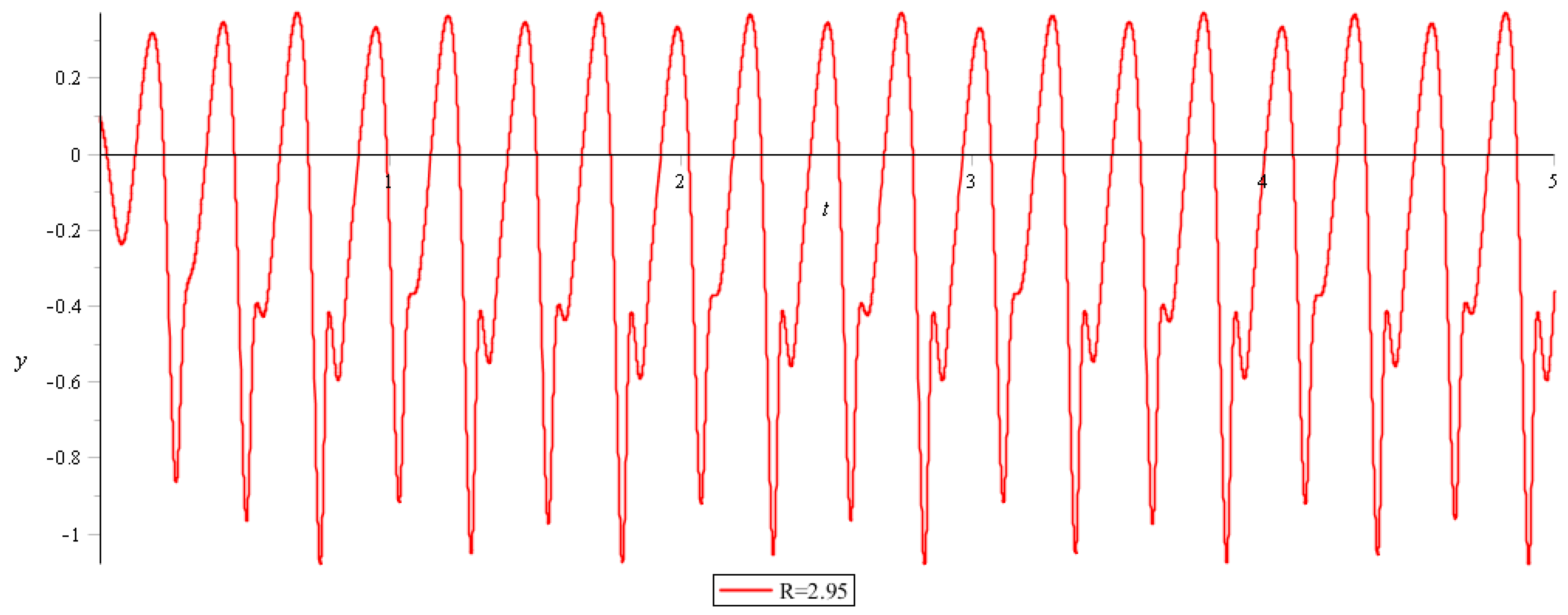
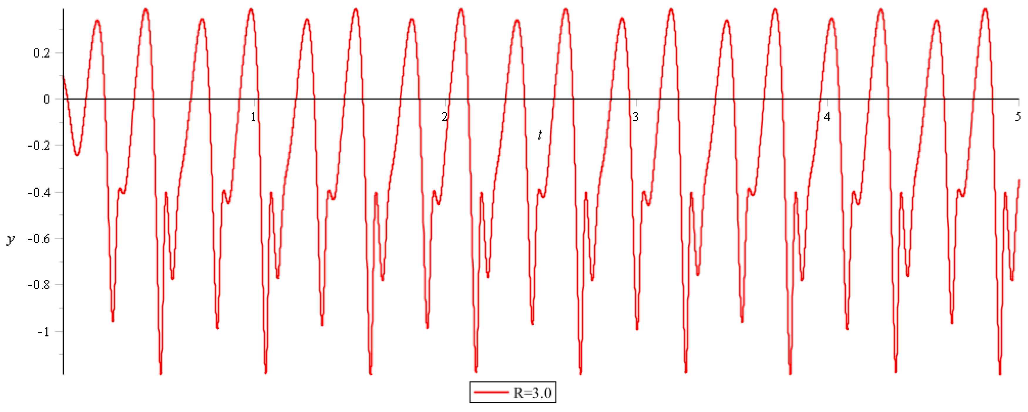
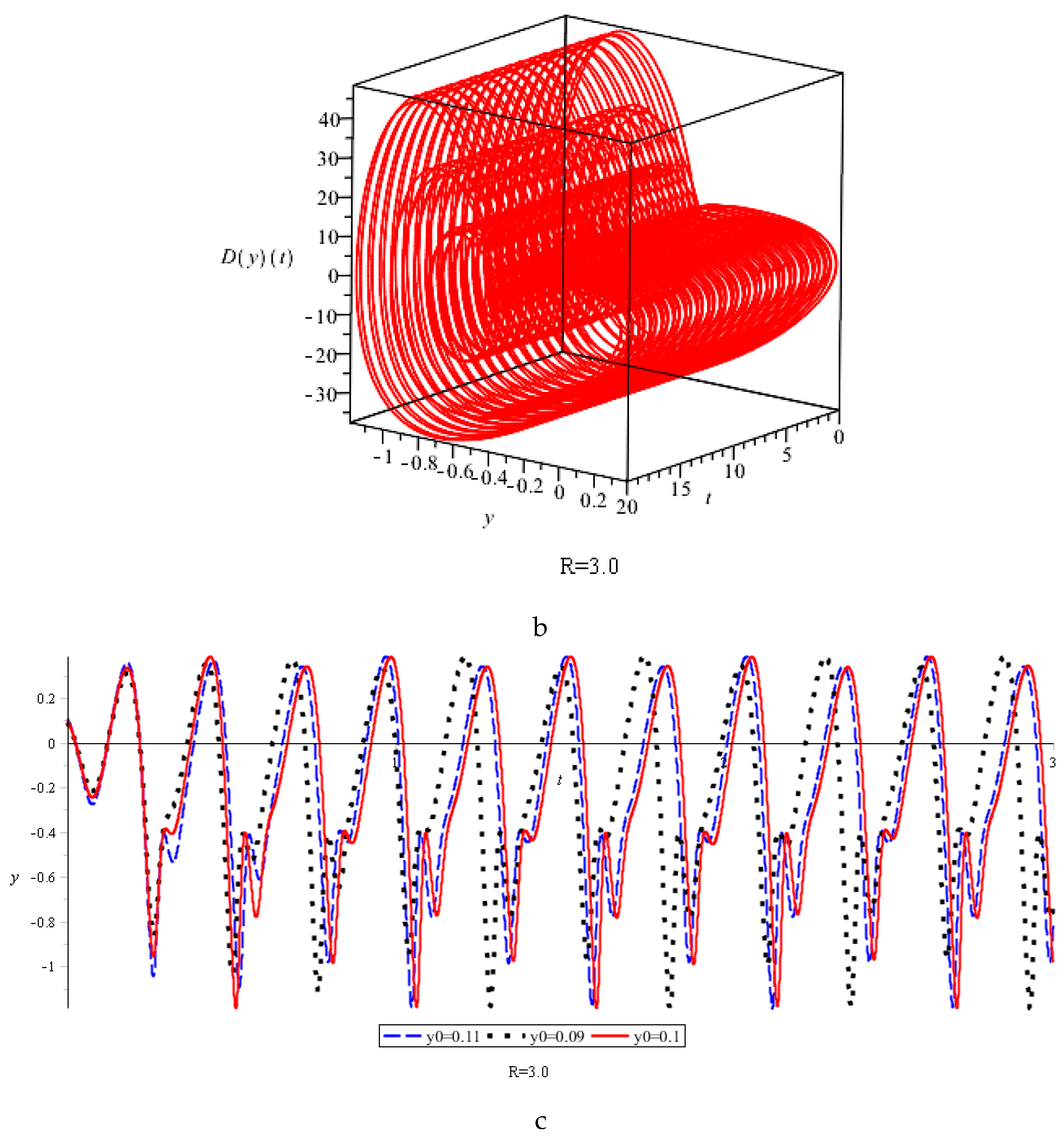
For the values
, a small change in the initial conditions does not lead to a radical change in the behavior of the system. For
in a periodic solution appears subharmonics (
Figure 4,
Figure 5 and
Figure 6).
In this case, with small changes in the initial conditions, the nature of oscillations of the system now undergoes significant changes (
Figure 6c).
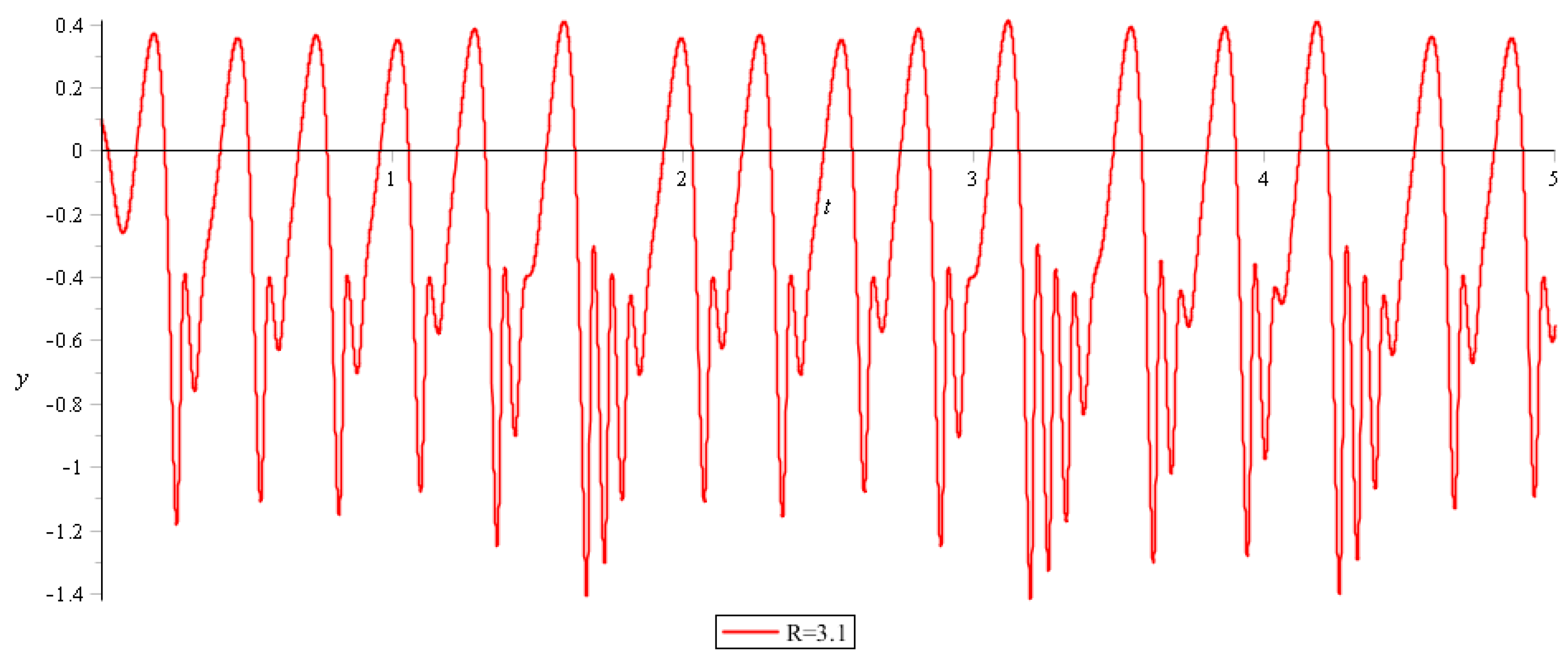
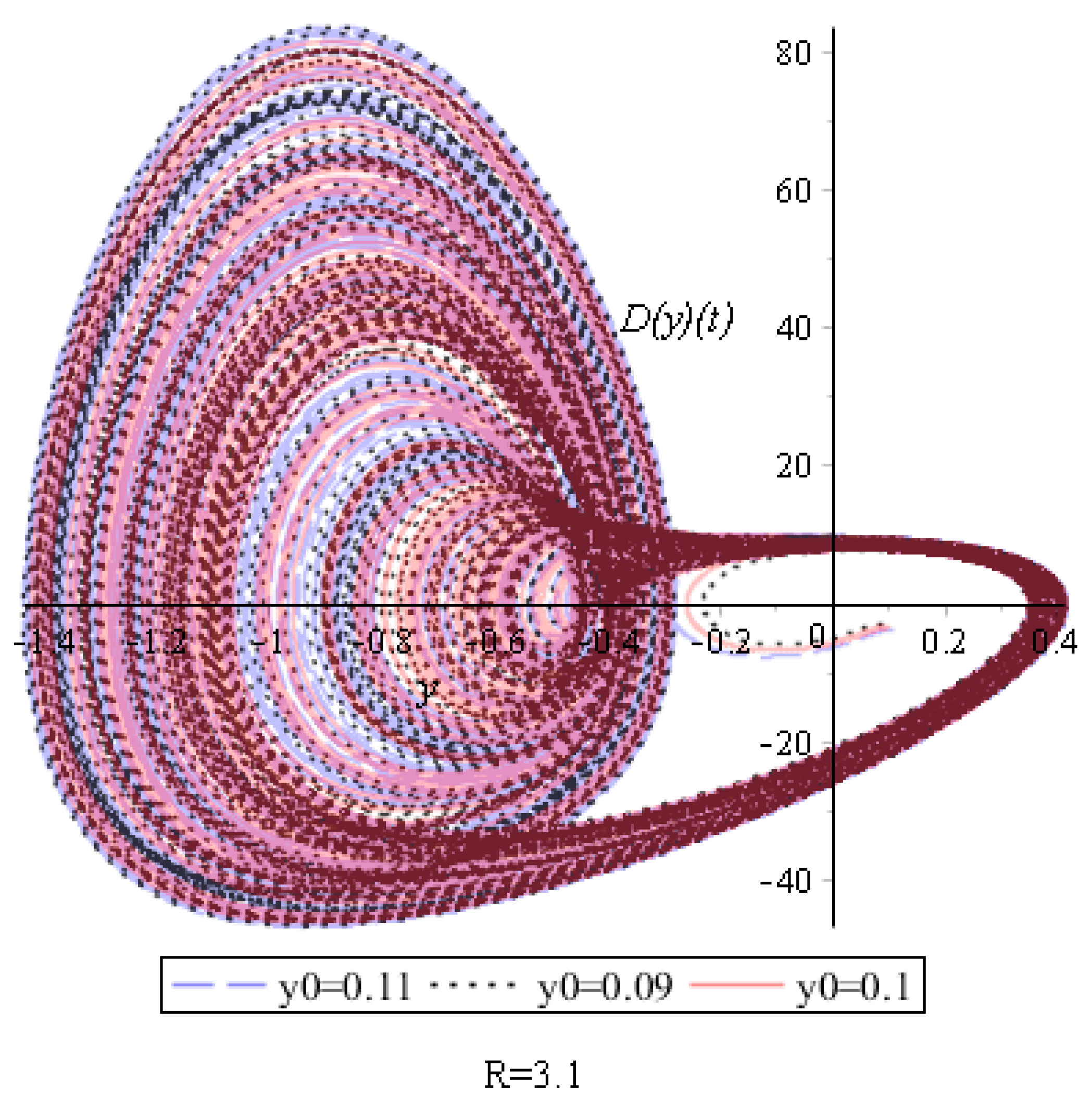
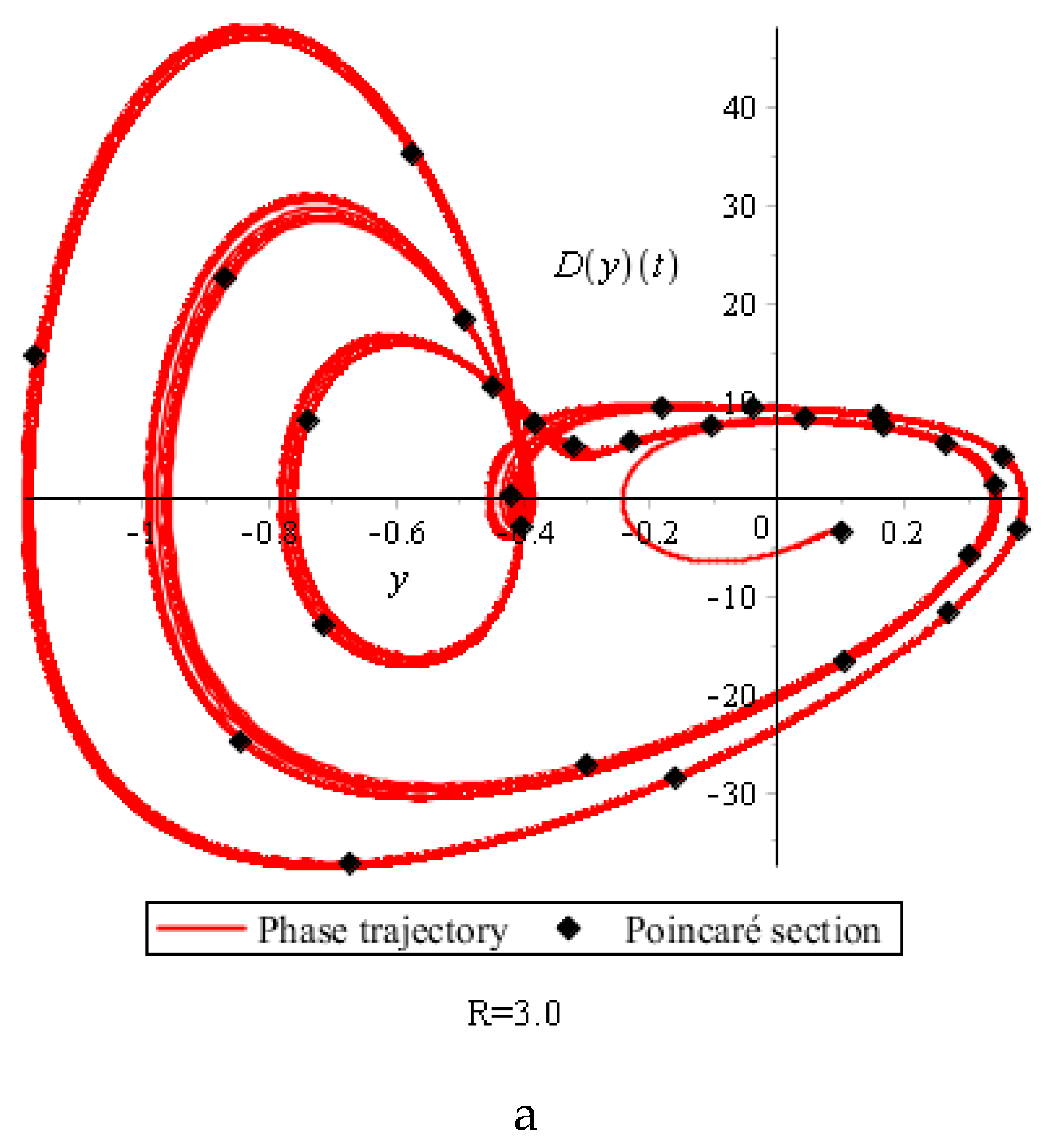
With the chaotic behavior of the system, small changes in the initial conditions lead to significant changes in the oscillations (
Figure 9c).
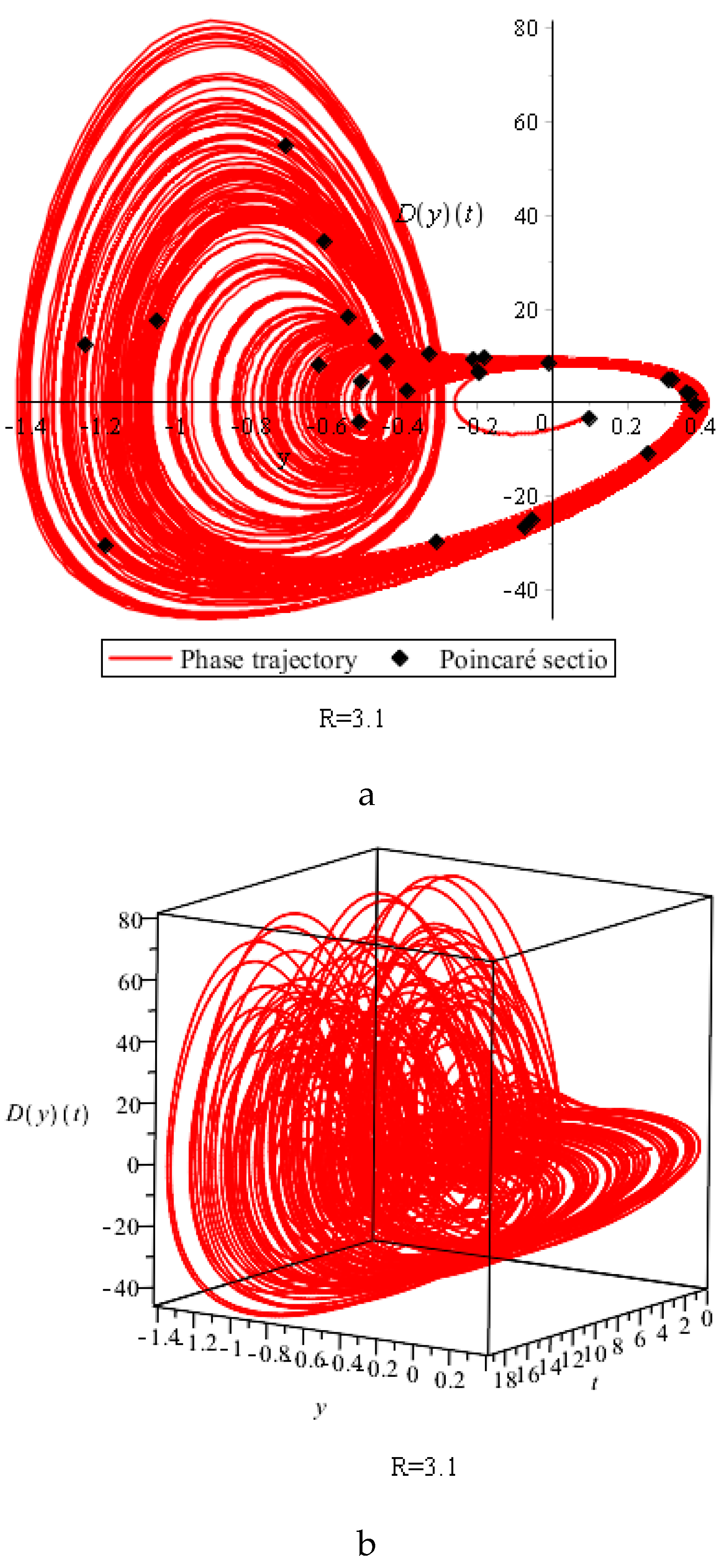
At the same time, phase trajectories with small changes in the initial conditions have a characteristic structure. If we exclude points that correspond to the initial mode of establishing oscillations, the structure of the phase trajectories does not depend on the initial conditions (
Figure 10 and
Figure 11).
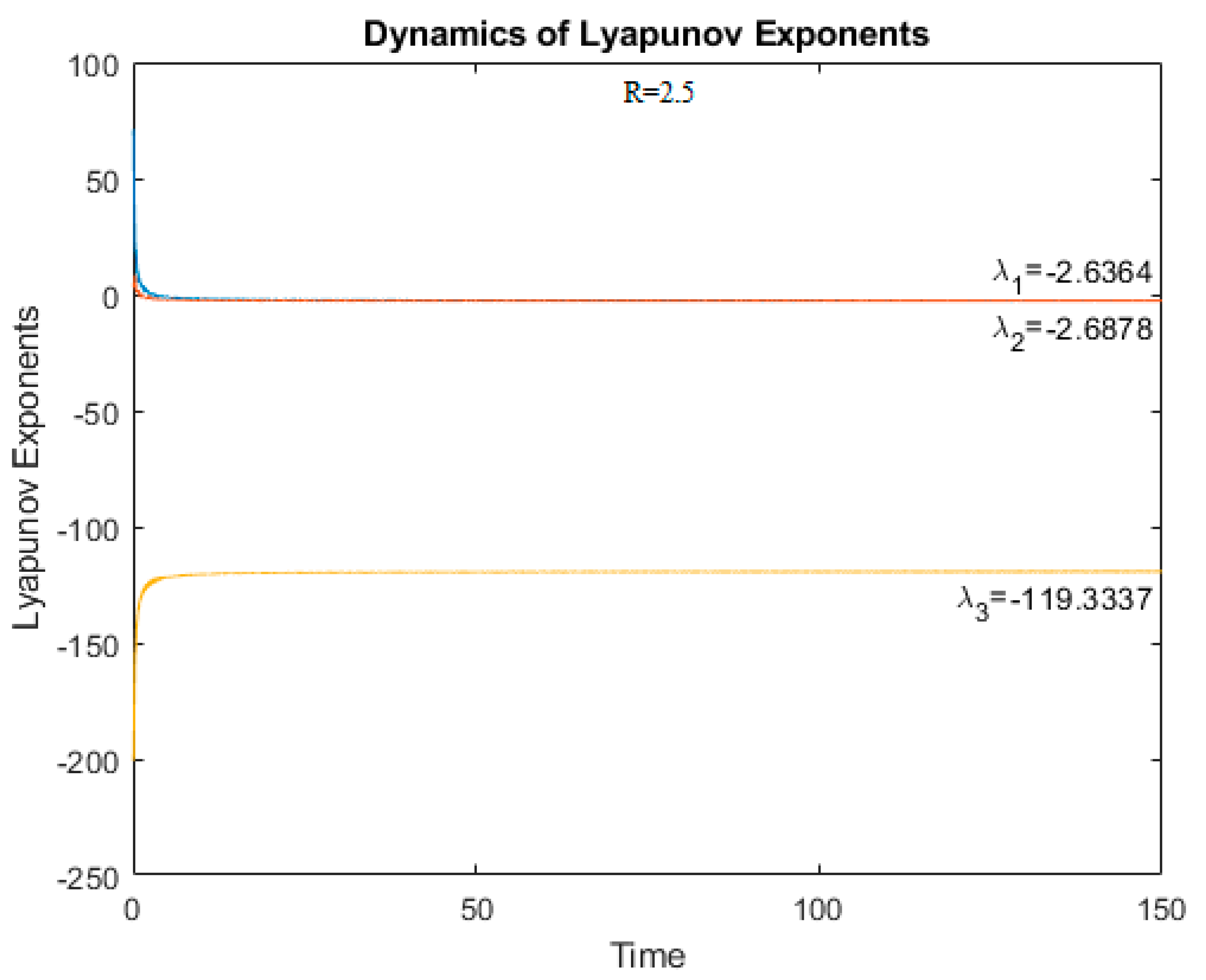
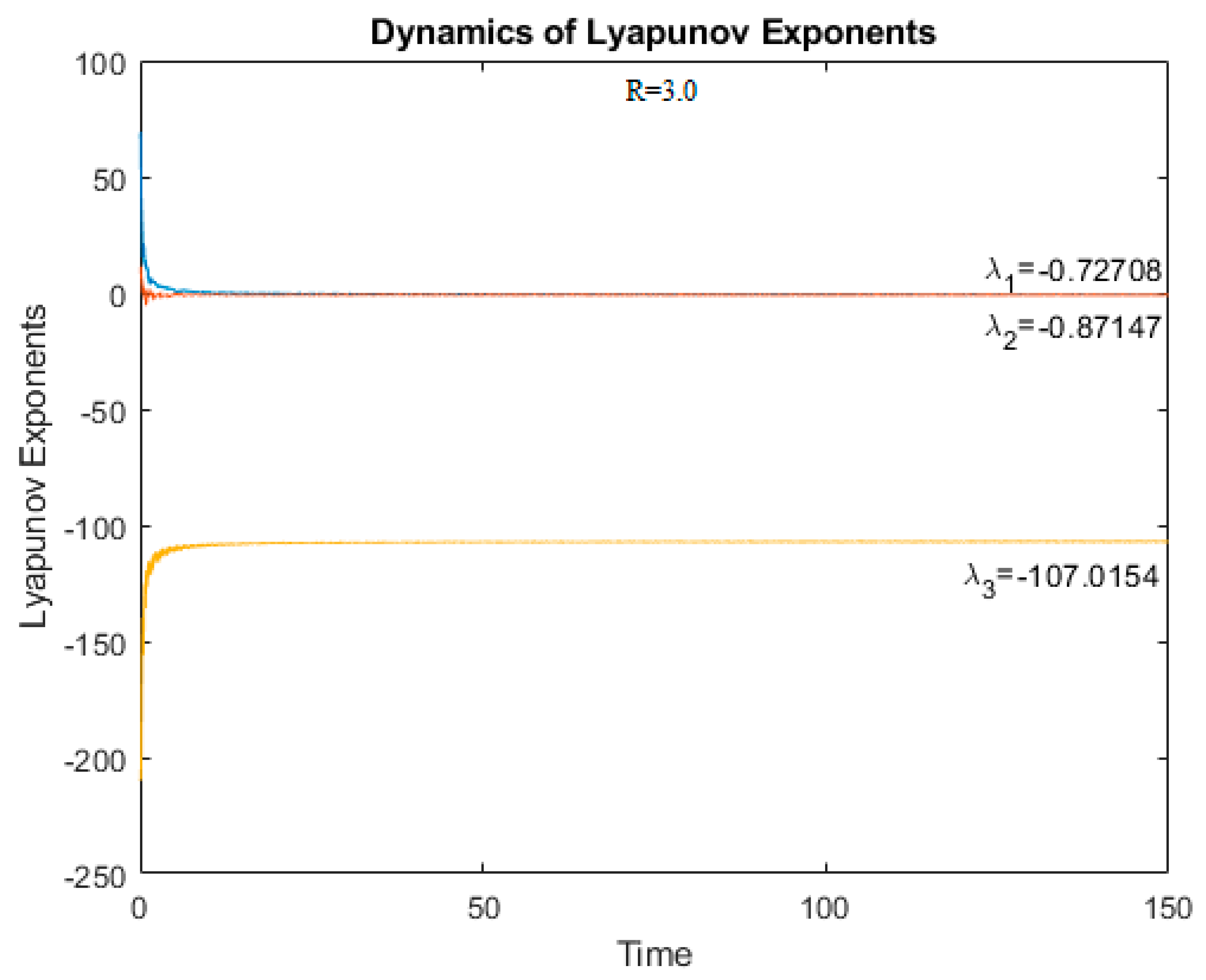
To correctly characterize the dynamics and confirmations of the chaotic behavior of the system we calculated for different values of R Lyapunov exponents and Lyapunov dimensions. If the system has at least one positive Lyapunov exponent, then it is chaotic [
5,
8,
9]. The multi-paradigm numerical computing environment MATLAB was used to calculate Lyapunov exponents.
Figure 12 and
Figure 13 show the dynamics of Lyapunov exponents for R = 2.5 and R = 3.0, respectively. Since all Lyapunov exponents are negative, the system is not chaotic.
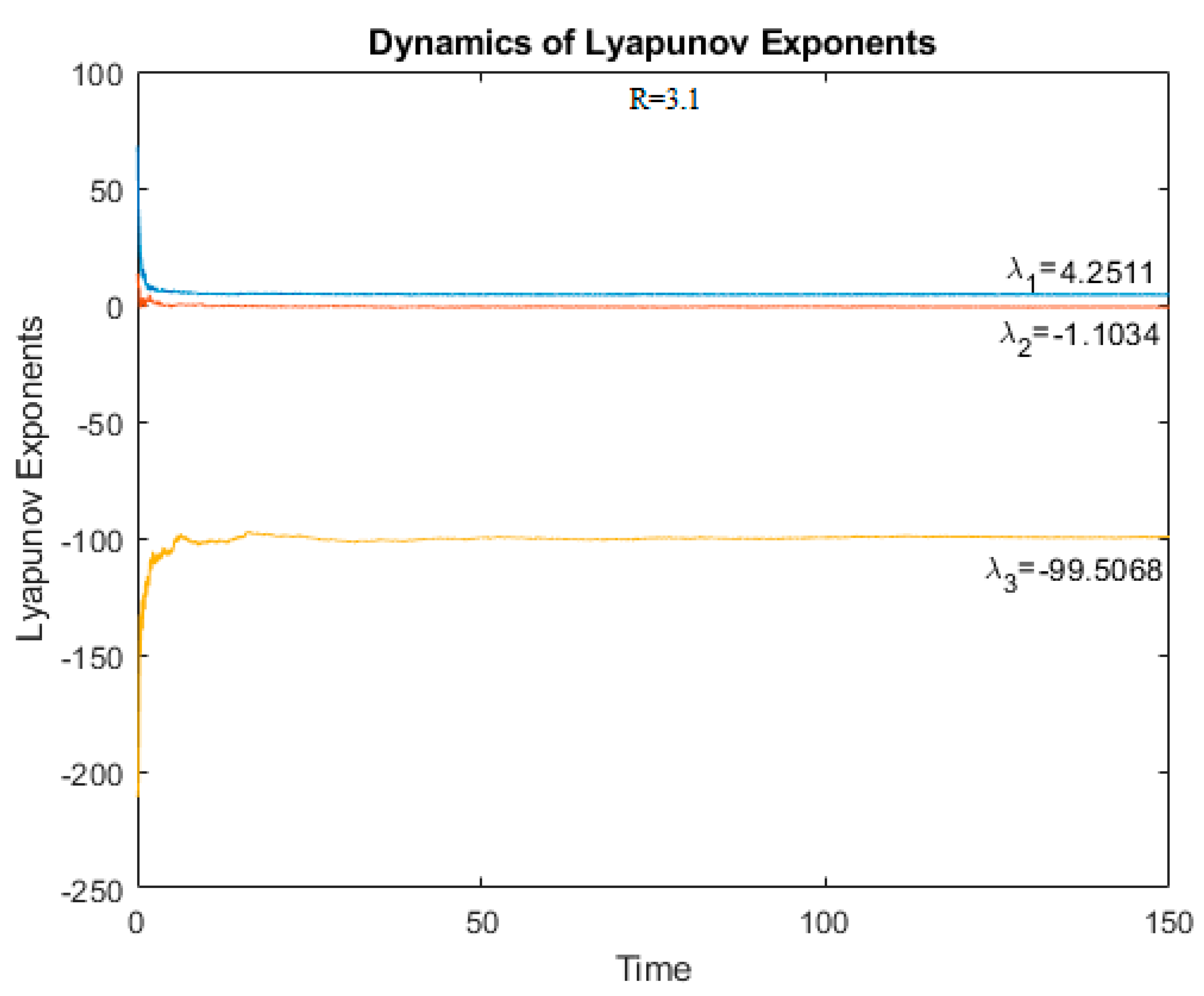
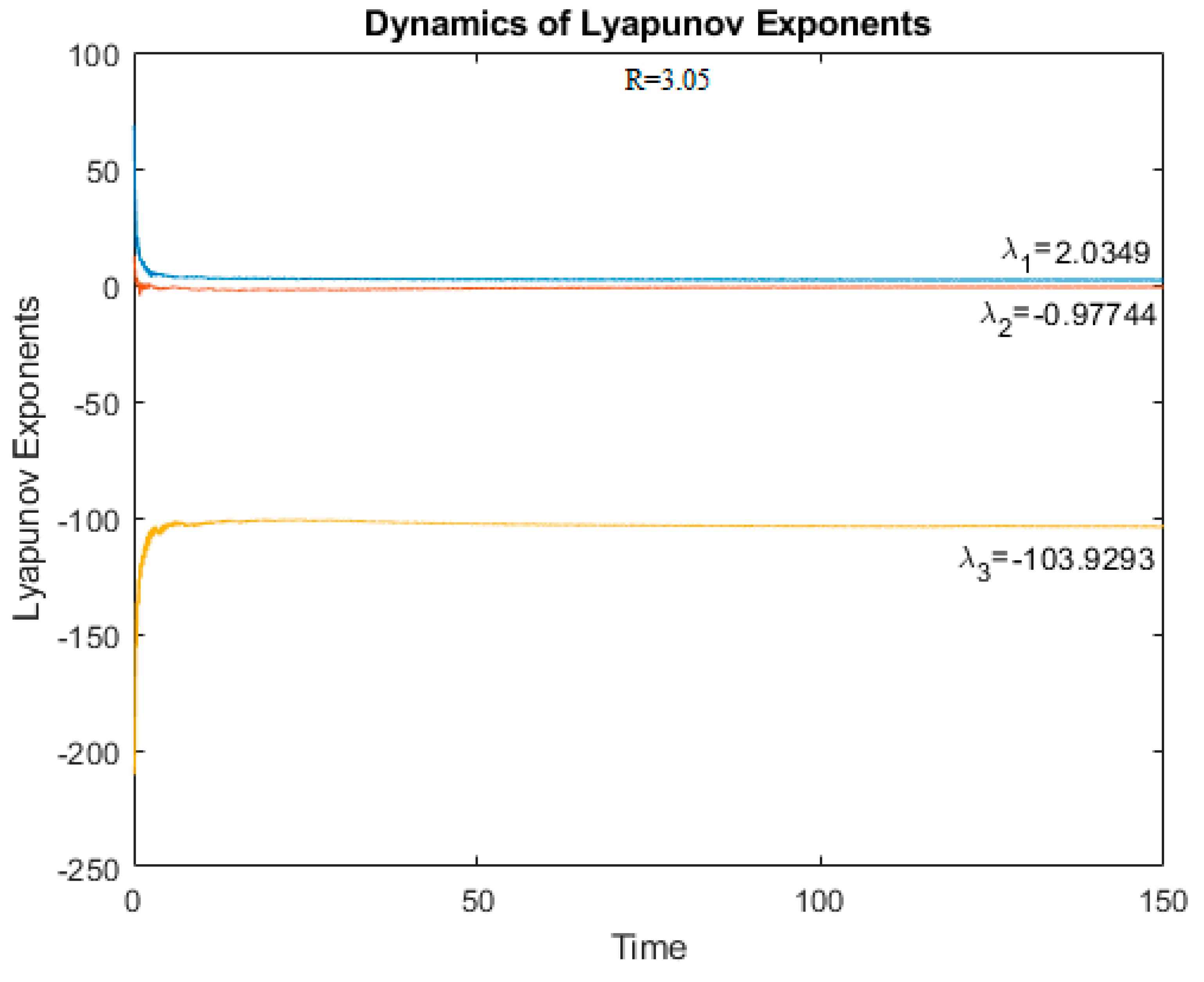
At R > 3.0, the largest Lyapunov exponent becomes positive, which indicates the appearance of chaos in the system (
Figure 14 and
Figure 15).
The obtained values of Lyapunov exponents confirm the earlier conclusions about the absence or presence of chaos in the system.
The Lyapunov dimension
can be calculated using the formula:
where
is defined from the conditions:
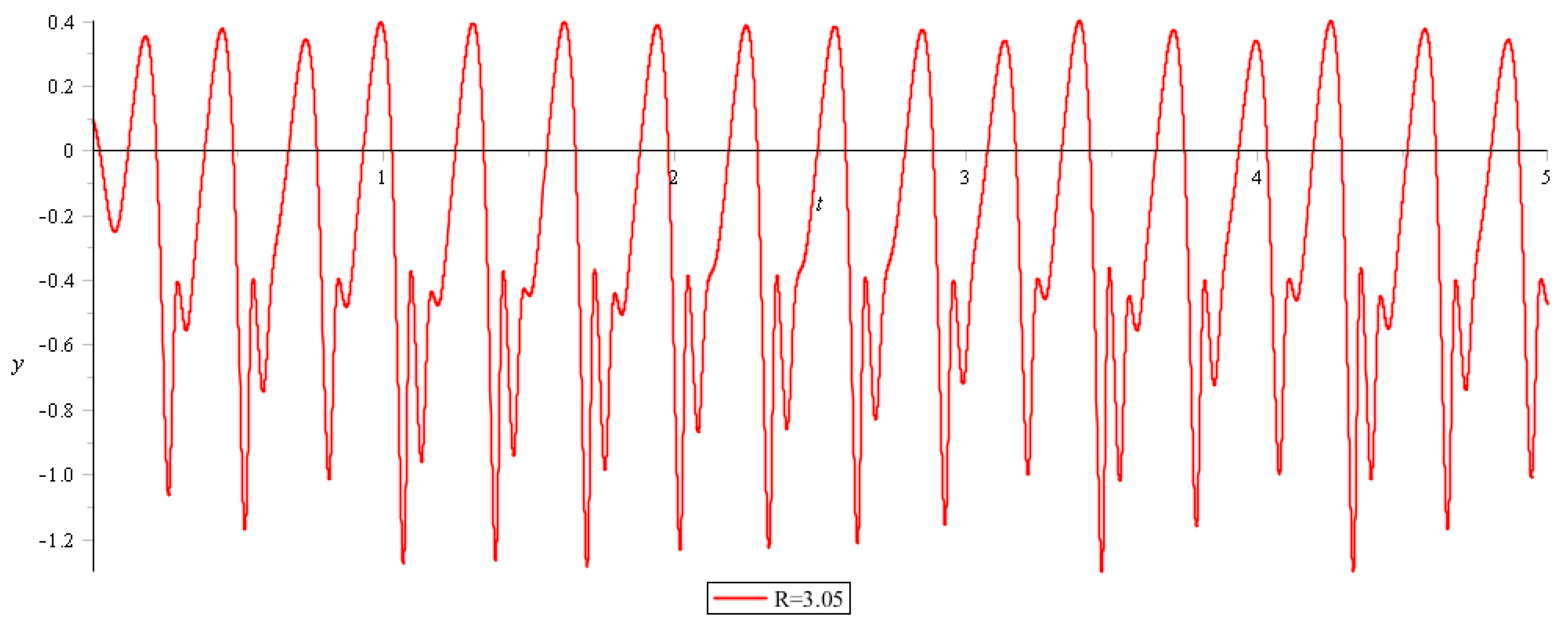
For R = 3.05 and R = 3.1 one obtains:
which are consistent with that of a third order chaotic system [
19].
5. Conclusions
Differential and difference equations are the main tools for mathematical modeling of physical, economic, environmental, social processes, and phenomena [
3,
4,
7]. To study differential equations, the entire arsenal of Calculus and Functional Analysis is used. Difference equations are the standard tools for numerical analysis. The relationship between these procedures is nontrivial, discretization or continualization often fundamentally change the nature of the solution. Therefore, the study of approaches that allow these operations to preserve the basic properties of the original systems is interesting. The question of discretization of differential equations preserving their properties has been well studied and continues to be studied. In our article, we briefly touch on this problem by the example of conservative discretization of the logistic equation. This question is closely related to group properties of the original ODE and O
E. We do not use such a deep theory, remaining within the framework of the phenomenological approach.
Our second task was to construct a continuous approximation of a discrete logistic equation with chaotic behavior. Continualization procedure was based on Padé approximants. To correctly characterize the dynamics of obtained ODE we measured such characteristic parameters of chaotic dynamical systems as the Lyapunov exponents and the Lyapunov dimensions.
