Second-Order Sliding Mode Formation Control of Multiple Robots by Extreme Learning Machine

Abstract

This paper addresses a second-order sliding mode control method for the formation problem of multirobot systems. The formation patterns are usually symmetrical. This sliding mode control is based on the super-twisting law. In many real-world applications, the robots suffer from a great diversity of uncertainties and disturbances that greatly challenge super-twisting sliding mode formation maneuvers. In particular, such a challenge has adverse effects on the formation performance when the uncertainties and disturbances have an unknown bound. This paper focuses on this issue and utilizes the technique of an extreme learning machine to meet this challenge. Within the leader–follower framework, this paper investigates the integration of the super-twisting sliding mode control method and the extreme learning machine. The output weights of this extreme learning machine are adaptively adjusted so that this integrated formation design has guaranteed closed-loop stability in the sense of Lyaponov. In the end, some simulations are implemented via a multirobot platform, illustrating the superiority and effectiveness of the integrated formation design in spite of uncertainties and disturbances.

1. Introduction

With the emergence of artificial intelligence technologies, multirobot systems have drawn great attention [1]. Such systems not only strengthen and refine the ability of individual robots, but they also provide a platform to display collective behaviors [2,3]. Compared with a complex robot, multirobot systems rooted in the real world have broad applications, for example, collaborative projects, military reconnaissance, and search and rescue [4,5].

In many industrial, agricultural, and maritime situations, multiple robots have to form up into some given patterns in order to fulfill a task [6]. In order to manage and coordinate the robots, the formation problem must be addressed. This problem originated in biological phenomena in nature, such as schools of fish swimming or a team of ants moving [7,8]. Concerning these biological systems, their formation behaviors exhibit high robustness and hierarchy in that a certain formation mechanism inherently exists. Similarly, the multiple robots call for such a mechanism. Some typical mechanisms have been developed for the robots, that is, the behavior-based algorithm, the virtual structure technique, the leader–follower framework, and the artificial potential field approach [9]. From the aspect of control design, the leader–follower framework has blossomed notably, although the mechanism is criticized for its drawback of a “single point of failure” [10]. This paper does not focus on how to design a novel mechanism, but it provides a formation control design. Consequently, the leader–follower framework was directly adopted because the mechanism is of merit for small- and medium-scale formation problems.

From the viewpoint of reality, the individual robots of a multirobot system are inevitably subject to uncertainties and disturbances which will make the formation dynamics of this multirobot system uncertain [11,12]. Affected by these adverse factors, the formation control problem of multiple robots becomes challenging. Many control strategies have been reported, i.e., iterative learning control [13,14], model predictive control [15], interval type-2 fuzzy control [16,17], and so on.

As a synthetic tool, sliding mode control is an alternative for the formation problem of uncertain multirobot systems. So far, some sliding-mode-based formation methods have been presented, that is, first-order sliding mode control [18,19], integral sliding mode control [8], derivative and integral terminal sliding mode control [4], and terminal sliding mode control [20]. Sliding mode control’s most attractive property is its invariance, which can guarantee that a sliding mode control system is completely robust despite the matched uncertainties and disturbances [21].

On the other side, sliding mode control is also confronted with the dilemma of chattering. As a result, many ideas have been devoted to the decrease and elimination of chattering. Among these ideas, the super-twisting-based sliding mode control technique is advocated because it only needs the information of a sliding mode variable and gets rid of the dependence on the time derivative of this sliding mode variable [22].

On the assumption that the bounds of uncertainties and disturbances are known, this technique is able to effectively force the sliding mode variable and its time derivative to the origin in finite time [23,24]. Unfortunately, this assumption is not mild in uncertain multirobot systems. In reality, one has to overestimate the bounds from the aspect of the closed-loop formation stability [25,26]. However, the overestimate definitely enlarges the gain of the super-twisting sliding mode control technique. A potential solution is to design a module that can adaptively estimate the bounds.

Motivated by this solution idea, some technical methods have been explored, i.e., disturbance observers, adaptive law design, fuzzy or neural network compensators, and so on. In this paper, the extreme learning machine (ELM) [27] is taken into consideration. The ELM is a kind of feed-forward neural network with a single hidden layer. The parameters in its hidden layer need no tuning, as they are generated randomly and independent of the training data. Compared with the back-propagation algorithm, the training and learning speed of the ELM is much faster. So far, the ELM has been successfully applied to microwave filters [28], traffic accident detection [29], air–fuel ratio control [30], and so on. However, application of the ELM technique to the formation problem of multi-agent mobile robots has not been reported. In this paper, we adopted the ELM for the super-twisting sliding mode formation maneuvers of uncertain multirobot systems. The purpose of this was to refine the formation performance when the bounds of the uncertainties and disturbances are unknown.

The highlights of the paper are summarized as follows.

• An architecture that combines second-order sliding mode control and the extreme learning machine technique is investigated.
• The closed-loop stability of this combination is presented in the sense of Lyapunov.
• Some numerical results for different formation patterns are demonstrated to support the combination.

The remainder of this paper is organized as follows. Section 2 models both a single mobile robot and a leader–follower pair. Section 3 addresses super-twisting sliding mode control, adopts an ELM to estimate the bounds of the uncertainties and disturbances, and analyzes the closed-loop formation stability in the sense of Lyapunov. In Section 4, we implement the presented control method in a multirobot system platform. Some numerical results and comparisons are illustrated in Section 4. Finally, conclusions are drawn in Section 5.

2. Formation Model

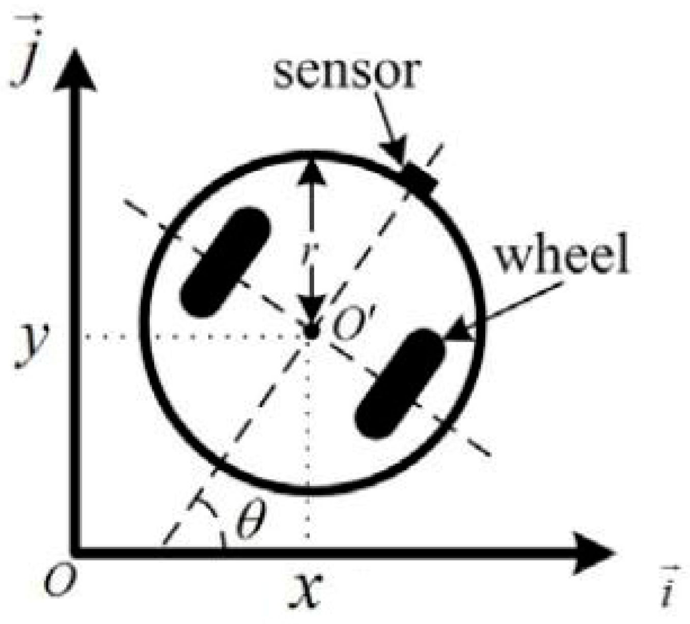
2.1. A Single Robot

Suppose there exists a unicycle-like robot, shown in Figure 1. The robot moves in the horizontal plane. It is round, and the diameter is 2r. Its two parallel wheels have the same axis and are independently controlled by two direct current motors. The robot can simultaneously rotate and translate, described by

$$q={\left[\begin{array}{ccc}x& y& \theta \end{array}\right]}^T.$$

(1)

In Equation (1), (x, y) is located at the center of the robot and represents its translational coordinates, and θ indicates its rotational coordinate. To know the position, a positioning sensor at the front castor of this robot is set up, as shown in Figure 1. The axis of the sensor is orthogonal to the axis of the two wheels.

On the assumption of pure rolling and no slipping, the ideal kinematic model of this robot [4,8] has the form

$$\dot{q}=\left[\begin{array}{c}\dot{x}\\ \dot{y}\\ \dot{\theta }\end{array}\right]=\left[\begin{array}{c}\begin{array}{cc}\cos \theta & 0\end{array}\\ \begin{array}{cc}\sin \theta & 0\end{array}\\ \begin{array}{cc}0& 1\end{array}\end{array}\right]·\left[\begin{array}{c}v\\ \omega \end{array}\right]$$

(2)

$$\mathrm{s}.\mathrm{t}.\dot{x}\sin \theta -\dot{y}\cos \theta =0$$

(3)

where $v$ is the robot’s linear velocity in the X–Y coordinates, and its direction is determined by the X–Y coordinates as well; $\omega$ represents the angular velocity, and its direction is positive when the robot rotates counterclockwise.

Concerning the constraint given by Equation (3), the time derivative of Equation (2), namely, the ideal dynamic model, can be written as

$$\left[\begin{array}{c}\ddot{x}\\ \ddot{y}\\ \ddot{\theta }\end{array}\right]=\left[\begin{array}{c}-\dot{y}\dot{\theta }\\ \dot{x}\dot{\theta }\\ 0\end{array}\right]+\left[\begin{array}{c}\begin{array}{cc}\cos \theta & 0\end{array}\\ \begin{array}{cc}\sin \theta & 0\end{array}\\ \begin{array}{cc}0& 1\end{array}\end{array}\right]·u$$

(4)

where $u={[\begin{array}{cc}\dot{v}& \dot{\omega }\end{array}]}^T$. The derivatives of $v$ and $\omega$ represent the acceleration and angular acceleration of the robot, respectively.

Since the robot in reality suffers from a variety of uncertainties and disturbances, for example, friction, slip and slide shift, and so forth, the real dynamic model [8] can be derived from Equation (4).

$$\left[\begin{array}{c}\ddot{x}\\ \ddot{y}\\ \ddot{\theta }\end{array}\right]=\left[\begin{array}{c}-\dot{y}\dot{\theta }\\ \dot{x}\dot{\theta }\\ 0\end{array}\right]+\left[\begin{array}{c}\begin{array}{cc}\cos \theta & 0\end{array}\\ \begin{array}{cc}\sin \theta & 0\end{array}\\ \begin{array}{cc}0& 1\end{array}\end{array}\right]·(u+\Delta ·u)+\pi \left(q,\dot{q}\right)$$

(5)

In Equation (5), the term $\pi \left(q,\dot{q}\right)$ represents the lumped uncertainties and disturbances, defined by

$$\pi \left(q,\dot{q}\right)={[\begin{array}{ccc}{\pi }_x& {\pi }_y& {\pi }_{\theta }\end{array}]}^T$$

where ${\pi }_x$, ${\pi }_y$, and ${\pi }_{\theta }$ are the functions of the vectors $q$ and $\dot{q}$. $\Delta$ indicates the physical parameter changes of this robot, described by

$$\Delta =\left[\begin{array}{cc}\epsilon & 0\\ 0& {\epsilon }^{\prime }\end{array}\right]$$

where $\epsilon$ and ${\epsilon }^{\prime }$ are the changes in the mass and the inertia of the robot, respectively.

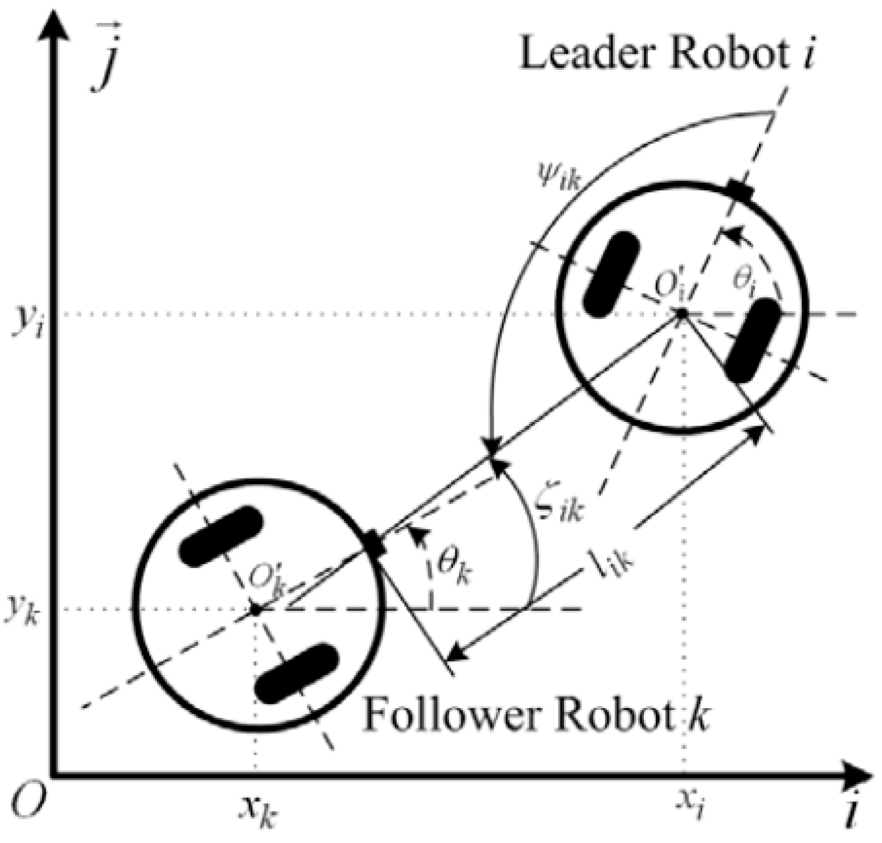
2.2. A Leader–Follower Pair

Consider a multirobot system containing N-many robots. Each robot is the same as the robot in Figure 1. Without loss of generality, the robot i is selected as the leader, and it makes up N − 1 leader–follower pairs with the remaining robots. Figure 2 illustrates such a leader–follower pair made up of the leader i and follower k [8].

In Figure 2, the subscript i is adopted to label the individual variables of the leader, the subscript k is employed to describe the individual variables of the follower, and the subscript ik is used for the relative variables for this pair. Here, the relative distance l_ik means the distance between the leader’s center and the follower’s front castor, formulated by

$$l_{ik}=\sqrt{{\left(x_i-{\overline{x}}_k\right)}^2+{\left(y_i-{\overline{y}}_k\right)}^2}$$

(6)

where

$$\begin{array}{l}{\overline{x}}_k=x_k+r\cos {\theta }_k\\ {\overline{y}}_k=y_k+r\sin {\theta }_k.\end{array}$$

The relative bearing angle ${\psi }_{ik}$ of the leader–follower pair is determined by

$${\psi }_{ik}=\pi +{\zeta }_{ik}-{\theta }_i$$

(7)

where

$${\zeta }_{ik}=\arctan \frac{y_i-y_k-r\sin {\theta }_k}{x_i-x_k-r\cos {\theta }_k}.$$

The purpose of this paper was to investigate the super-twisting sliding mode formation maneuvers of this multirobot system via an extreme learning machine. Motivated by this purpose, the formation objective of the leader–follower scheme was that each leader–follower pair of the multirobot system has to keep the desired relative distance and the desired relative bearing angle in spite of uncertainties and disturbances. In order to focus on the objective, we considered some ideal conditions as follows: (1) there are neither collisions nor communication delay; (2) the follower is well known, that is, it knows its position and velocity, and it can obtain the position and velocity of the leader as well.

We define a vector x_ik = [x₁ x₂ x₃ x₄]^T. Let $x_1=l_{ik}$, $x_2={\dot{l}}_{ik}$, $x_3={\psi }_{ik}$, and $x_4={\dot{\psi }}_{ik}$. According to the formation objective, the relative distance $l_{ik}$ and the relative bearing angle ${\psi }_{ik}$ are determined as the formation control output. Then, the formation dynamics of this leader–follower pair among the multiple robots can have the form of Equation (8) in light of the leader–follower scheme.

$$\begin{array}{l}{\dot{x}}_{ik}=f\left(x_{ik},d_{ik}\right)+g\left(x_{ik},{\Delta }_k\right)u_k,\\ y_{ik}=h\left(x_{ik}\right).\end{array}$$

(8)

Here, x_ik is the system state vector and y_ik is the system output vector. Further,

$$\begin{gathered} f\left(x_{ik},d_{ik}\right)=A_{ik}{x}_{ik}+B_{ik,2}{d}_{ik}, \\ g\left(x_{ik},{\Delta }_k\right)=B_{ik,1}+B_{ik,1}{\Delta }_k. \end{gathered}$$

A_ik, B_ik,1, B_ik,2 and h(x_ik) are defined as

$$A_{ik}=\left[\begin{array}{cccc}0& 1& 0& 0\\ 0& 0& 0& 0\\ 0& 0& 0& 1\\ 0& 0& 0& 0\end{array}\right],B_{ik,2}=\left[\begin{array}{c}\begin{array}{cc}0& 0\end{array}\\ \begin{array}{cc}1& 0\end{array}\\ \begin{array}{cc}0& 0\end{array}\\ \begin{array}{cc}0& 1\end{array}\end{array}\right],B_{ik,1}=\left[\begin{array}{c}\begin{array}{cc}0& 0\end{array}\\ \begin{array}{cc}\cos {\phi }_{ik}& r\sin {\phi }_{ik}\end{array}\\ \begin{array}{cc}0& 0\end{array}\\ \begin{array}{cc}\frac{-\sin {\phi }_{ik}}{l_{ik}}& \frac{r\cos {\phi }_{ik}}{l_{ik}}\end{array}\end{array}\right],h\left(x_{ik}\right)=\left[\begin{array}{c}{x}_1\\ x_3\end{array}\right],$$

where ${\phi }_{ik}={\psi }_{ik}+{\theta }_{ik}$. $d_{ik}$ is the lumped term of all the uncertainties and disturbances in the leader–follower pair.

$$d_{ik}=L_{ik}\left(I_2+{\Delta }_i\right)u_i+F_{ik}+P_{ik}$$

(9)

In Equation (9),

$$L_{ik}=\left[\begin{array}{cc}0& 0\\ -\cos {\psi }_{ik}& 0\\ 0& 0\\ \frac{\sin {\psi }_{ik}}{l_{ik}}& -1\end{array}\right],F_{ik}=\left[\begin{array}{c}0\\ F_1\\ 0\\ F_2\end{array}\right],P_{ik}=\left[\begin{array}{c}0\\ P_1\\ 0\\ P_2\end{array}\right]$$

where $I_2$ is a 2 × 2 identity matrix and F₁, F₂, P₁, and P₂ are written as

$$\begin{gathered} \begin{array}{ll}{F}_1& ={({\dot{\psi }}_{ik})}^2{l}_{ik}+2{\dot{\psi }}_{ik}{\dot{\theta }}_i{l}_{ik}+{({\dot{\theta }}_i)}^2{l}_{ik}\\ & -r\cos {\phi }_{ik}{({\dot{\theta }}_k)}^2-({\dot{y}}_k{\dot{\theta }}_k-{\dot{y}}_i{\dot{\theta }}_i)\cos ({\psi }_{ik}+{\dot{\theta }}_i)-({\dot{x}}_i{\dot{\theta }}_i-{\dot{x}}_k{\dot{\theta }}_k)\sin ({\psi }_{ik}+{\theta }_i)\end{array} \\ \begin{array}{ll}{F}_2& =\frac{-({\dot{y}}_k{\dot{\phi }}_{ik}-{\dot{\psi }}_{ik}{\dot{y}}_i)\sin ({\psi }_{ik}+{\theta }_i)-r{\dot{\theta }}_k{\dot{\phi }}_{ik}\sin {\phi }_{ik}}{l_{ik}}\\ & \frac{-({\dot{x}}_k{\dot{\phi }}_{ik}-{\dot{\psi }}_{ik}{\dot{x}}_i)\cos ({\psi }_{ik}+{\theta }_i)+i_{ik}(({\dot{y}}_i-{\dot{y}}_k)\cos ({\psi }_{ik}+{\theta }_i)-({\dot{x}}_i-{\dot{x}}_k)\sin ({\psi }_{ik}+{\theta }_{{}_i})-r{\dot{\theta }}_k{\dot{\phi }}_{ik}\cos {\phi }_{ik})}{l_{ik}}\end{array} \\ {P}_1=-({\pi }_{ix}-{\pi }_{kx})\cos ({\psi }_{ik}+{\theta }_i)-({\pi }_{iy}-{\pi }_{ky})sin({\psi }_{ik}+{\theta }_i)+r{\pi }_{k\theta }\sin {\phi }_{ik} \\ {P}_2=\frac{({\pi }_{ix}-{\pi }_{kx})sin({\psi }_{ik}+{\theta }_i)-({\pi }_{iy}-{\pi }_{ky})\cos ({\psi }_{ik}+{\theta }_i)+r{\pi }_{k\theta }\sin {\phi }_{ik}-l_{ik}{\pi }_{i\theta }}{l_{ik}}. \end{gathered}$$

The formation dynamics in Equation (8) are depicted by first-order differential equations. Further, the formation dynamics can also be written using second-order differential equations,

$${\ddot{\mathbb{T}}}_{ik}={\mathbb{G}}_{ik}{u}_k+{\mathbb{D}}_{ik}$$

(10)

Here,

$$\begin{gathered} {\mathbb{T}}_{ik}={\left[\begin{array}{cc}{l}_{ik}& {\psi }_{ik}\end{array}\right]}^T.{\mathbb{G}}_{ik}=\left[\begin{array}{cc}\cos {\phi }_{ik}& r\sin {\phi }_{ik}\\ -\frac{\sin {\phi }_{ik}}{l_{ik}}& \frac{r\cos {\phi }_{ik}}{l_{ik}}\end{array}\right], \\ {\mathbb{D}}_{ik}={\left[\begin{array}{cc}{d}_{ik,1}& d_{ik,2}\end{array}\right]}^T={\mathbb{G}}_{ik}{\Delta }_k{u}_k+{\mathbb{L}}_{ik}(I_2+{\Delta }_i)u_i+{\mathbb{F}}_{ik}+{\mathbb{P}}_{ik}, \\ {\mathbb{L}}_{ik}=\left[\begin{array}{cc}-\cos {\psi }_{ik}& 0\\ \frac{\sin {\psi }_{ik}}{l_{ik}}& -1\end{array}\right],{\mathbb{F}}_{ik}=\left[\begin{array}{c}{F}_1\\ F_2\end{array}\right],{\mathbb{P}}_{ik}=\left[\begin{array}{c}{P}_1\\ P_2\end{array}\right]. \end{gathered}$$

Both Equations (8) and (10) describe the formation dynamics, where Equation (8) is in the form of first-order differential equations and Equation (9) is expressed in second-order differential equations. Inherently, they are equivalent to each other, and both of them can help the following control design.

3. Formation Control Design

3.1. Sliding Surfaces and Input–Output Dynamics

The super-twisting law is a powerful and effective technique that can realize a second-order sliding mode control design. The technique can effectively deal with a controlled plant with a relative degree equal to 1 with respect to the control input. With regard to the matched uncertainties and disturbances, it can make the sliding mode variable and its time derivative converge to the origin in finite time. Consequently, we considered this technique as a solution for formation maneuvers of the leader–follower pair in Figure 2. In order to implement the control design, the sliding surfaces, that is, the sliding-mode vector, have to be predefined.

$$s_{ik}=\left[\begin{array}{c}{s}_{ik,1}\\ s_{ik,2}\end{array}\right]=C_1\left(\left[\begin{array}{c}{l}_{ik}\\ {\psi }_{ik}\end{array}\right]-\left[\begin{array}{c}{l}_{ik}^d\\ {\psi }_{ik}^d\end{array}\right]\right)+C_2\left(\left[\begin{array}{c}{\dot{l}}_{ik}\\ {\dot{\psi }}_{ik}\end{array}\right]-\left[\begin{array}{c}{\dot{l}}_{ik}^d\\ {\dot{\psi }}_{ik}^d\end{array}\right]\right)$$

(11)

Here, $l_{ik}^d$ and ${\psi }_{ik}^d$ are the desired relative distance and the desired relative bearing angle, respectively, of the leader–follower pair. $C_1$ and $C_2$ are 2 × 2 constant diagonal matrices, given by

$$C_1=\left[\begin{array}{cc}{c}_1& 0\\ 0& c_1\end{array}\right]\mathrm{and}{C}_2=\left[\begin{array}{cc}{c}_2& 0\\ 0& c_2\end{array}\right]$$

where both $c_1$ and $c_2$ are positive and predefined constants.

We differentiate the sliding-mode vector $s_{ik}$ in Equation (11) with respect to time and substitute the formation dynamics Equation (8) into the derivative of $s_{ik}$. Then, the input–output dynamics are determined by

$${\dot{s}}_{ik}=\frac{\partial s_{ik}}{\partial t}+\frac{\partial s_{ik}}{\partial x_{ik}}f\left(x_{ik},d_{ik}\right)+\frac{\partial s_{ik}}{\partial x_{ik}}g\left(x_{ik},{\Delta }_k\right)u_k.$$

(12)

In order to achieve a super-twisting sliding mode control design, the first step is to calculate the relative degree of the dynamics via Equation (11) with respect to the control input. From Equations (11) and (12), we have

$$\frac{\partial s_{ik}}{\partial u_k}=0\mathrm{and}\frac{\partial {\dot{s}}_{ik}}{\partial u_k}=\frac{\partial s_{ik}}{\partial x_{ik}}g\left(x_{ik},{\Delta }_k\right)\ne 0.$$

(13)

From Equation (13), it is apparent that the relative degree of $s_{ik}$ with respect to $u_k$ is equal to 1. In other words, a super-twisting sliding mode control design is available for the formation maneuvers of multiple robots under the leader–follower scheme.

Let

$$\begin{array}{l}a(x_{ik},d_{ik},t)=\frac{\partial s_{ik}}{\partial t}+\frac{\partial s_{ik}}{\partial x_{ik}}f\left(x_{ik},d_{ik}\right),\\ b(x_{ik},{\Delta }_k,t)=\frac{\partial s_{ik}}{\partial x_{ik}}g\left(x_{ik},{\Delta }_k\right).\end{array}$$

(14)

Assumption 1.

The matrix$b(x_{ik},{\Delta }_k,t)\in {\Re }^{2\times 2}$in Equation (14) contains both known and unknown parts, written as

$$b(x_{ik},{\Delta }_k,t)=b_0(x_{ik},t)+b_1(x_{ik},{\Delta }_k,t).$$

(15)

Here, $b_0(x_{ik},t)$ is a known positively definite matrix, $b_1(x_{ik},{\Delta }_k,t)$ is bounded but unknown, and the two parts of $b(x_{ik},{\Delta }_k,t)$ satisfy

$$\Vert b_1(x_{ik},{\Delta }_k,t)b_0^{-1}(x_{ik},t){\Vert }_2<{\gamma }_1<1$$

(16)

where ${\gamma }_1$ is a unknown constant.

Assumption 2.

The vector$a(x_{ik},d_{ik},t)\in {\Re }^{2\times 1}$contains both known and unknown parts, depicted by

$$a(x_{ik},d_{ik},t)=a_0(x_{ik},t)+a_1(x_{ik},d_{ik},t).$$

(17)

Here, $a_0(x_{ik},t)$ is a known and bounded vector and $a_1(x_{ik},d_{ik},t)$ is bounded but unknown. Their ∞-norms satisfy

$$\Vert a_0(x_{ik},t){\Vert }_{\infty }\le {\delta }_1\sqrt{\Vert s_{ik}{\Vert }_2}\mathrm{and}\Vert {\dot{a}}_1(x_{ik},d_{ik},t){\Vert }_{\infty }\le {\delta }_2$$

(18)

where ${\delta }_1$ and ${\delta }_2$ are positive but unknown.

Concerning the two assumptions, the input–output dynamics of the sliding-mode vector $s_{ik}$ in Equations (12) can have the form

$${\dot{s}}_{ik}=a_0+b_0{u}_k+a_1+b_1{u}_k.$$

(19)

Here, $a_0(x_{ik},t)$, $a_1(x_{ik},d_{ik},t)$, $b_0(x_{ik},t)$, and $b_1(x_{ik},{\Delta }_k,t)$ are abbreviated to $a_0$, $a_1$, $b_0$, and $b_1$ for brevity.

3.2. Super-Twisting Sliding Mode Control Design

According to the nominal system in Equation (19), the super-twisting sliding mode control can be designed as

$$u_k=b_0^{-1}(-a_0+{\varpi }_k)$$

(20)

where

$$\begin{gathered} {\varpi }_k={\varpi }_{k1}+{\varpi }_{k2}, \\ {\varpi }_{k1}=-{\alpha }_k\sqrt{\Vert s_{ik}{\Vert }_2}\mathrm{sgn}(s_{ik}), \\ {\dot{\varpi }}_{k2}=-{\chi }_k\mathrm{sgn}(s_{ik}). \end{gathered}$$

(21)

In (21), ${\alpha }_k$ and ${\chi }_k$ are positive and they need to be predefined. The signum function $\mathrm{sgn}(s_{ik})$ in Equation (22) is defined by $\mathrm{sgn}(s_{ik})={\left[\begin{array}{cc}\mathrm{sgn}(s_{ik,1})& \mathrm{sgn}(s_{ik,2})\end{array}\right]}^T$. We select a Lyapunov function candidate

$$V_0={\Vert s_{ik}\Vert }_2.$$

(22)

We consider the input–output dynamics in Equation (19) and substitute Equations (20) and (21) into Equation (19). Given Assumptions 1 and 2, the time derivative of Equation (22) has the following form:

$$\begin{array}{ll}{\dot{V}}_0& =\frac{s_{ik}^T{\dot{s}}_{ik}}{{\Vert s_{ik}\Vert }_2}=\frac{s_{ik}^T}{{\Vert s_{ik}\Vert }_2}(a_0+b_0{u}_k+a_1+b_1{u}_k)\\ & =\frac{s_{ik}^T}{{\Vert s_{ik}\Vert }_2}\left[{\varpi }_k+a_1+b_1{b}_0^{-1}(-a_0+{\varpi }_k)\right]\\ & =\frac{s_{ik}^T}{{\Vert s_{ik}\Vert }_2}\left[\left(-{\alpha }_k-{\alpha }_k{b}_1{b}_0^{-1}\right)\sqrt{\Vert s_{ik}{\Vert }_2}\mathrm{sgn}(s_{ik})+\left(-{\chi }_k-{\chi }_k{b}_1{b}_0^{-1}\right){\displaystyle {\int }_0^t\mathrm{sgn}(s_{ik})\mathrm{d}t}+a_1-b_1{b}_0^{-1}{a}_0\right]\\ & \le \frac{s_{ik}^T}{{\Vert s_{ik}\Vert }_2}\left[\left(-{\alpha }_k+{\alpha }_k{\gamma }_1\right)\sqrt{\Vert s_{ik}{\Vert }_2}\mathrm{sgn}(s_{ik})+\left(-{\chi }_k+{\chi }_k{\gamma }_1\right){\displaystyle {\int }_0^t\mathrm{sgn}(s_{ik})\mathrm{d}t}+a_1+{\gamma }_1{a}_0\right]\\ & =\frac{\left(-{\alpha }_k+{\alpha }_k{\gamma }_1\right)\sqrt{\Vert s_{ik}{\Vert }_2}}{{\Vert s_{ik}\Vert }_2}{s}_{ik}^T\mathrm{sgn}(s_{ik})+\frac{\left(-{\chi }_k+{\chi }_k{\gamma }_1\right)}{{\Vert s_{ik}\Vert }_2}{s}_{ik}^T{\displaystyle {\int }_0^t\mathrm{sgn}(s_{ik})\mathrm{d}t}+\frac{s_{ik}^T}{{\Vert s_{ik}\Vert }_2}\left(a_1+{\gamma }_1{a}_0\right).\end{array}$$

(23)

Note that the following equalities exist.

$${\Vert s_{ik}\Vert }_1=s_{ik}^T\mathrm{sgn}(s_{ik})\mathrm{and}{\displaystyle {\int }_0^t\mathrm{sgn}(s_{ik})\mathrm{d}t}=\mathrm{sgn}(s_{ik}){\displaystyle {\int }_0^t\mathrm{d}t}$$

(24)

Considering (18), (23) can be written as

$$\begin{array}{ll}{\dot{V}}_0& \le \frac{\left(-{\alpha }_k+{\alpha }_k{\gamma }_1\right)\sqrt{\Vert s_{ik}{\Vert }_2}}{{\Vert s_{ik}\Vert }_2}{\Vert s_{ik}\Vert }_1+\frac{s_{ik}^T}{{\Vert s_{ik}\Vert }_2}\gamma a_0+\frac{{\Vert s_{ik}\Vert }_1}{{\Vert s_{ik}\Vert }_2}{\displaystyle {\int }_0^t\left(-{\chi }_k+{\chi }_k{\gamma }_1\right)}dt+\frac{s_{ik}^T}{{\Vert s_{ik}\Vert }_2}{\displaystyle {\int }_0^t{\dot{a}}_1}dt\\ & \le \frac{\left(-{\alpha }_k+{\alpha }_k{\gamma }_1\right)\sqrt{\Vert s_{ik}{\Vert }_2}}{{\Vert s_{ik}\Vert }_2}{\Vert s_{ik}\Vert }_1+{\gamma }_1{\delta }_1\frac{\sqrt{\Vert s_{ik}{\Vert }_2}}{{\Vert s_{ik}\Vert }_2}{\Vert s_{ik}\Vert }_1+\frac{{\Vert s_{ik}\Vert }_1}{{\Vert s_{ik}\Vert }_2}{\displaystyle {\int }_0^t\left(-{\chi }_k+{\chi }_k{\gamma }_1\right)\mathrm{d}t}+\frac{{\Vert s_{ik}\Vert }_1}{{\Vert s_{ik}\Vert }_2}{\displaystyle {\int }_0^t{\delta }_2\mathrm{d}t}\\ & =\frac{\sqrt{\Vert s_{ik}{\Vert }_2}{\Vert s_{ik}\Vert }_1}{{\Vert s_{ik}\Vert }_2}\left(-{\alpha }_k+{\alpha }_k{\gamma }_1+{\gamma }_1{\delta }_1\right)+\frac{{\Vert s_{ik}\Vert }_1}{{\Vert s_{ik}\Vert }_2}{\displaystyle {\int }_0^t\left(-{\chi }_k+{\chi }_k{\gamma }_1+{\delta }_2\right)\mathrm{d}t}.\end{array}$$

(25)

Concerning Equation (16), $0<{\gamma }_1<1$. Consequently, one can have ${\dot{V}}_0<0$ by picking up ${\alpha }_k$ and ${\chi }_k$ if ${\gamma }_1$, ${\delta }_1$, and ${\delta }_2$ are known. Unfortunately, these constants are hardly known in advance, that is, Equation (25) theoretically holds true but it is not available in reality. In order to make Equation (25) hold true, one possible approach is to overestimate ${\alpha }_k$ and ${\chi }_k$ so that ${\dot{V}}_0<0$ can be guaranteed and the closed-loop formation system can have stability in the sense of Lyapunov. However, the approach inevitably enlarges the gain of the super-twisting sliding mode control technique, which can definitely have adverse effects on the formation performance. To address this issue, in this paper we selected the extreme learning machine and fused it with super-twisting sliding mode control. Their integration can guarantee the formation stability while the super-twisting sliding mode control technique can have a suitable gain.

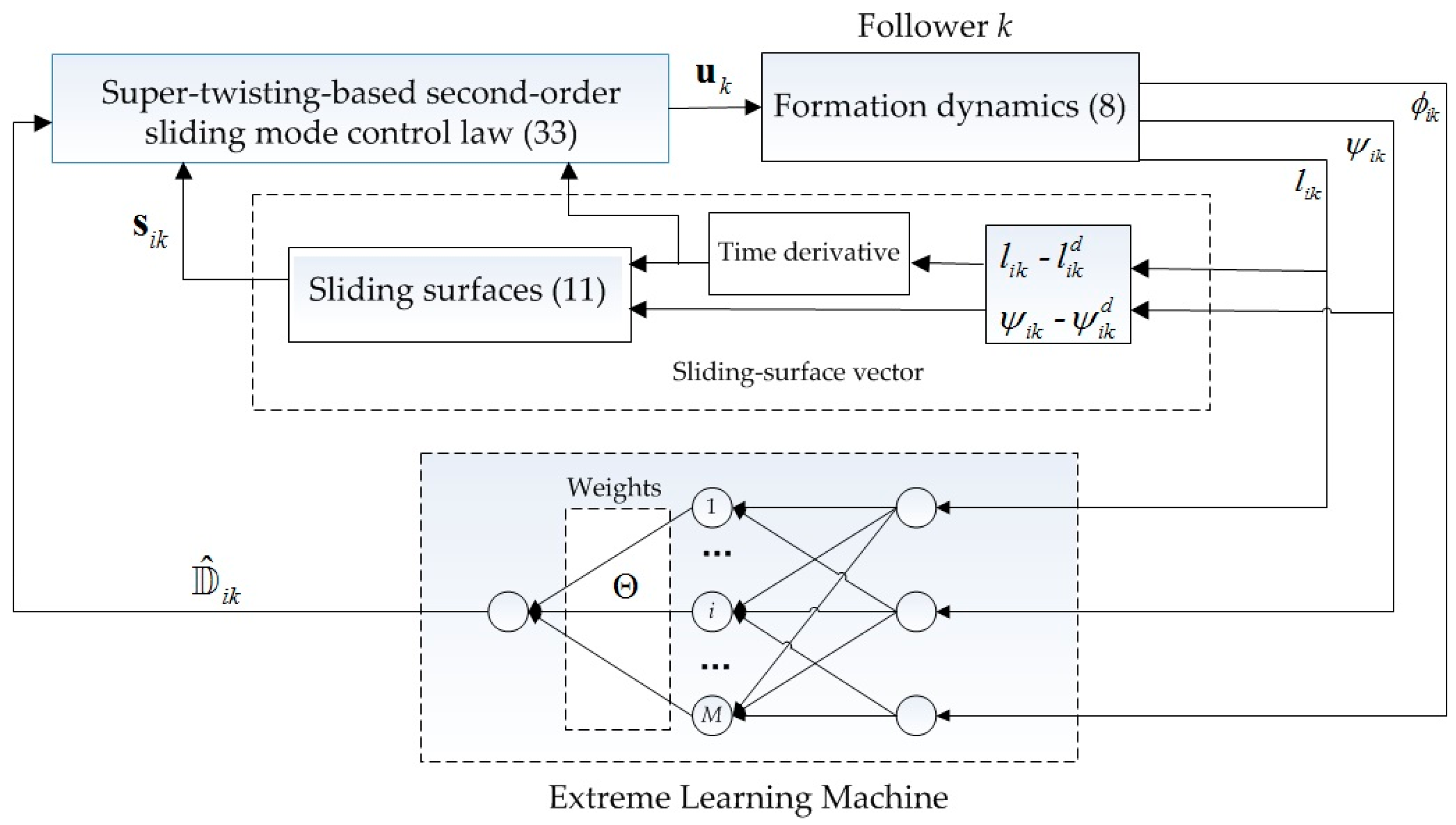
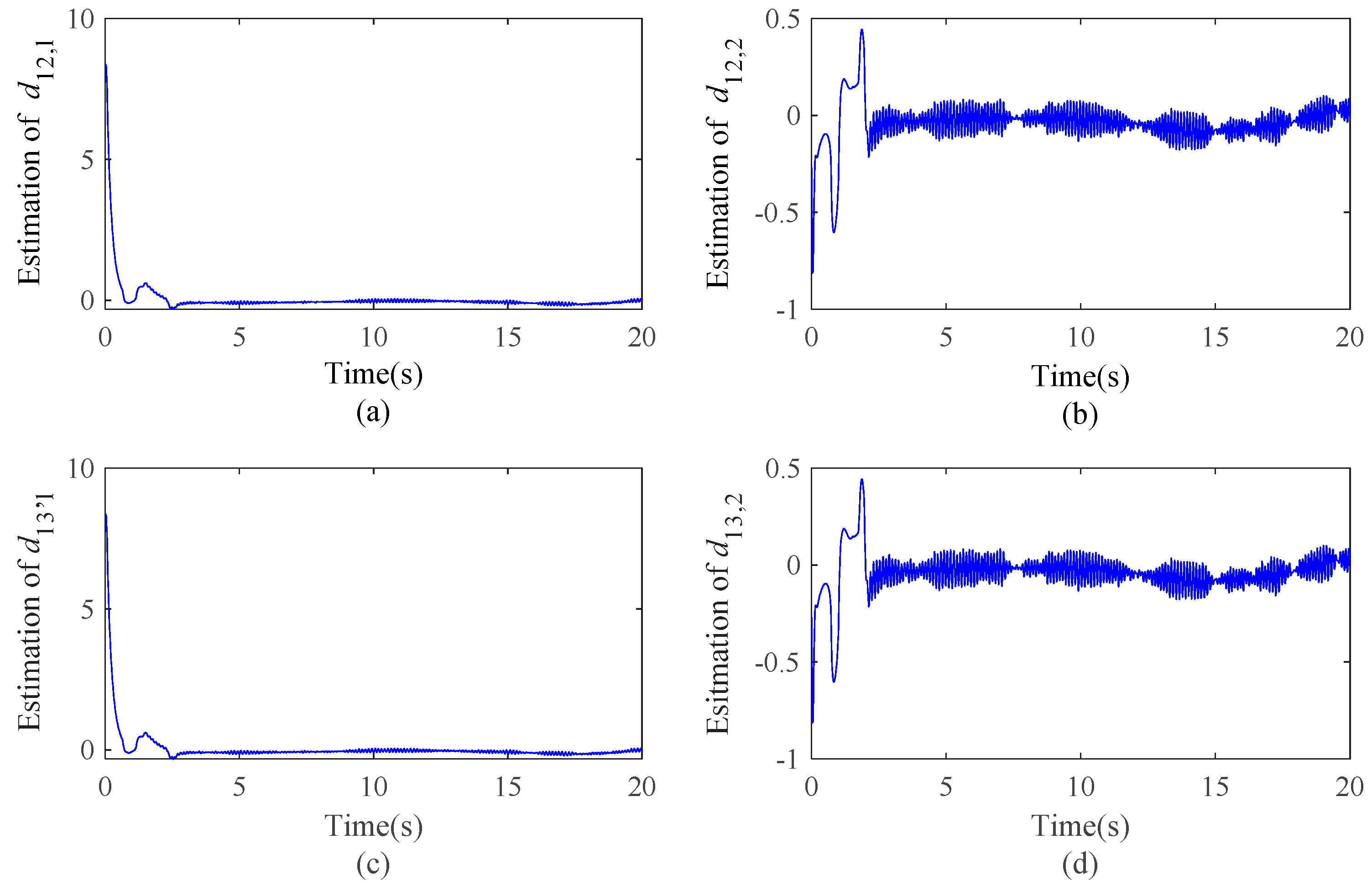
3.3. Super-Twisting Sliding Mode Control Design via ELM

The ELM is a learning algorithm for single-hidden-layer feed-forward networks. By the algorithm, the input weights are randomly chosen, the hidden layer biases are randomly assigned, and the output weights are analytically determined. The reason why the gain of the super-twisting sliding mode is overestimated is that some bounds are unknown. With the help of the ELM, one possible approach is to estimate these uncertainties and disturbance online, which can avoid the drawback of overestimating the bounds.

Considering the formation dynamics in the form of the second-order differential equations in Equation (10), the sliding surfaces in Equation (11) can be written as

$$s_{ik}=C_1\left({\mathbb{T}}_{ik}-{\mathbb{T}}_{ik}^d\right)+C_2\left({\dot{\mathbb{T}}}_{ik}-{\dot{\mathbb{T}}}_{ik}^d\right).$$

(26)

Then, the time derivative of Equation (26) is determined by

$${\dot{s}}_{ik}=C_1\left({\dot{\mathbb{T}}}_{ik}-{\dot{\mathbb{T}}}_{ik}^d\right)+C_2\left({\ddot{\mathbb{T}}}_{ik}-{\ddot{\mathbb{T}}}_{ik}^d\right).$$

(27)

For the formation maneuvers with constants $l_{ik}^d$ and ${\psi }_{ik}^d$, we have

$${\dot{\mathbb{T}}}_{ik}^d={\ddot{\mathbb{T}}}_{ik}^d={\left[\begin{array}{cc}0& 0\end{array}\right]}^T.$$

(28)

Consequently, Equation (27) has the form

$${\dot{s}}_{ik}=C_1{\dot{\mathbb{T}}}_{ik}+C_2{\ddot{\mathbb{T}}}_{ik}.$$

(29)

Substituting Equation (10) into Equation (29) yields

$${\dot{s}}_{ik}=C_1{\dot{\mathbb{T}}}_{ik}+C_2{\mathbb{G}}_{ik}{u}_k+C_2{\mathbb{D}}_{ik}.$$

(30)

Let

$${\dot{s}}_{ik}=C_1{\dot{\mathbb{T}}}_{ik}+C_2{\mathbb{G}}_{ik}{u}_k+C_2{\mathbb{D}}_{ik}={\varpi }_k$$

(31)

where ${\varpi }_k$ is defined in Equation (21). Then, $u_k$ can be obtained by

$$u_k={\left(C_2{\mathbb{G}}_{ik}\right)}^{-1}\left(-C_1{\dot{\mathbb{T}}}_{ik}-C_2{\mathbb{D}}_{ik}+{\varpi }_k\right).$$

(32)

From Equation (10), ${\mathbb{D}}_{ik}$ contains all the uncertainties and disturbances. Here the ELM is designed to estimate ${\mathbb{D}}_{ik}$ in real time. Replacing ${\mathbb{D}}_{ik}$ by its estimate ${\widehat{\mathbb{D}}}_{ik}$ in Equation (32) yields

$$u_k={\left(C_2{\mathbb{G}}_{ik}\right)}^{-1}\left(-C_1{\dot{\mathbb{T}}}_{ik}-C_2{\widehat{\mathbb{D}}}_{ik}+{\varpi }_k\right).$$

(33)

In Equation (9), ${\mathbb{D}}_{ik}$ is the function of some variables, where ${\phi }_{ik}$, $l_{ik}$, and ${\psi }_{ik}$ play an important role. Here, the three variables were chosen as the input nodes of the ELM, that is, $z\in {\Re }^{3\times 1}$ is the input vector and $z={\left[\begin{array}{ccc}{l}_{ik}& {\psi }_{ik}& {\phi }_{ik}\end{array}\right]}^T$. Without doubt, the output vector is just ${\widehat{\mathbb{D}}}_{ik}\in {\Re }^{2\times 1}$, that is, there are two output nodes located at the output layer.

We assigned M hidden nodes as the hidden layer. Then, the weights between the input and hidden layers can be defined by $w\in {\Re }^{M\times 3}$. The input bias vector of the hidden nodes was defined as $c\in {\Re }^{M\times 1}$. A sigmoidal function was selected as the activation function of the hidden layer. Then, the output of the lth $(l=1,2,\cdots ,M)$ hidden layer node can be calculated by

$$h_l(w_l·z+c_l)=\frac{1}{1+e^{-(w_l·z+c_l)}}.$$

(34)

Here, $w_l\in {\Re }^{1\times 3}$ is the lth row of $w$ and $c_l$ is the lth element of $c_l$.

The output weights between the hidden layer nodes and the output layer nodes were defined as $\Theta =\left[\begin{array}{cc}{\Theta }_1& {\Theta }_2\end{array}\right]\in {\Re }^{M\times 2}$, ${\Theta }_1\in {\Re }^{M\times 1}$, and ${\Theta }_2\in {\Re }^{M\times 1}$. Finally, the output vector of the ELM can be calculated by

$${\widehat{\mathbb{D}}}_{ik}={\Theta }^Tℍ.$$

(35)

Here, $ℍ={[\begin{array}{cccccc}{h}_1& h_2& \cdots & h_l& \cdots & h_M\end{array}]}^T$.

According to the universal approximation theorem of the single-hidden-layer feed-forward networks in [27], there exist optimal output weights ${\Theta }^{*}\in {\Re }^{M\times 2}$ to approximate ${\mathbb{D}}_{ik}$ so that

$${\mathbb{D}}_{ik}={\Theta }^{*T}ℍ+\epsilon (z)$$

(36)

where $\epsilon (z)\in {\Re }^{2\times 1}$ is an approximation error vector, and it can be arbitrarily reduced by increasing the number of hidden layer nodes. Therefore, it is assumed that

$${\Vert \epsilon (z)\Vert }_{\infty }<\overline{\epsilon }$$

(37)

where $\overline{\epsilon }$ is an arbitrary small constant.

Finally, a schematic diagram of the super-twisting second-order sliding mode formation control by the extreme learning machine is presented in Figure 3.

Theorem 1.

Consider the formation dynamics in Equations (8) and (10) given Assumptions 1 and 2, utilizing the super-twisting sliding mode control in Equation (33). Suppose the ELM is designed to estimate${\widehat{\mathbb{D}}}_{ik}$online by Equation (35). If the weights between the hidden and output layers of the ELM are adjusted by Equation (38), then the formation control system is asymptotically stable.

$${\dot{\Theta }}_q=\eta \frac{c_2}{{\Vert s_{ik}\Vert }_2}{s}_{ik,q}ℍq=1,2$$

(38)

Here, $\eta$ is a positive constant, and both $c_2$ and $s_{ik,q}$ are defined by Equation (11).

Proof. 

Take the following Lyapunov function candidate into consideration.

$$V={\Vert s_{ik}\Vert }_2+\frac{1}{2\eta }{\displaystyle \sum _{q=1}^2{\tilde{\Theta }}_q^T{\tilde{\Theta }}_q}$$

(39)

Here, $\tilde{\Theta }=\left[\begin{array}{cc}{\tilde{\Theta }}_1& {\tilde{\Theta }}_2\end{array}\right]$ is defined by

$$\tilde{\Theta }={\Theta }^{*}-\Theta .$$

(40)

The time derivative of $V$ can have the form of

$$\dot{V}=\frac{s_{ik}^T{\dot{s}}_{ik}}{{\Vert s_{ik}\Vert }_2}+\frac{1}{\eta }{\displaystyle \sum _{q=1}^2{\tilde{\Theta }}_q^T{\dot{\tilde{\Theta }}}_q}.$$

(41)

Substituting Equation (30) into Equation (41) yields

$$\dot{V}=\frac{s_{ik}^T}{{\Vert s_{ik}\Vert }_2}(C_1{\dot{\mathbb{T}}}_{ik}+C_2{\mathbb{G}}_{ik}{u}_k+C_2{\mathbb{D}}_{ik})+\frac{1}{\eta }{\displaystyle \sum _{q=1}^2{\tilde{\Theta }}_q^T{\dot{\tilde{\Theta }}}_q}.$$

(42)

Then, according to the designed formation control Equation (33), we have

$$\begin{array}{ll}\dot{V}& =\frac{s_{ik}^T}{{\Vert s_{ik}\Vert }_2}(C_2{\mathbb{D}}_{ik}-C_2{\widehat{\mathbb{D}}}_{ik}+{\varpi }_k)+\frac{1}{\eta }{\displaystyle \sum _{q=1}^2{\tilde{\Theta }}_q^T{\dot{\tilde{\Theta }}}_q}\\ & =\frac{s_{ik}^T}{{\Vert s_{ik}\Vert }_2}[C_2({\Theta }^{*T}ℍ-\epsilon (z))-C_2({\Theta }^Tℍ)+{\varpi }_k]+\frac{1}{\eta }{\displaystyle \sum _{q=1}^2{\tilde{\Theta }}_q^T{\dot{\tilde{\Theta }}}_q}\\ & =\frac{s_{ik}^T}{{\Vert s_{ik}\Vert }_2}[C_2({\Theta }^{*T}-{\Theta }^T)ℍ-C_2\epsilon (z)+{\varpi }_k]+\frac{1}{\eta }{\displaystyle \sum _{q=1}^2{\tilde{\Theta }}_q^T{\dot{\tilde{\Theta }}}_q}\\ & =\frac{s_{ik}^T}{{\Vert s_{ik}\Vert }_2}[C_2{\dot{\tilde{\Theta }}}^Tℍ-C_2\epsilon (z)+{\varpi }_k]+\frac{1}{\eta }{\displaystyle \sum _{q=1}^2{\tilde{\Theta }}_q^T{\dot{\tilde{\Theta }}}_q}\end{array}$$

(43)

From Equation (21), we can obtain

$$\begin{array}{ll}\dot{V}& =\frac{s_{ik}^T}{{\Vert s_{ik}\Vert }_2}\left[C_2{\tilde{\Theta }}^Tℍ-C_2\epsilon (z)-{\alpha }_k\sqrt{\Vert s_{ik}{\Vert }_2}\mathrm{sgn}(s_{ik})-{\displaystyle {\int }_0^t{\chi }_k\mathrm{sgn}(s_{ik})\mathrm{d}t}\right]+\frac{1}{\eta }{\displaystyle \sum _{q=1}^2{\tilde{\Theta }}_q^T{\dot{\tilde{\Theta }}}_q}\\ & =\frac{s_{ik}^T}{{\Vert s_{ik}\Vert }_2}{C}_2{\tilde{\Theta }}^Tℍ+\frac{1}{\eta }{\displaystyle \sum _{q=1}^2{\tilde{\Theta }}_q^T{\dot{\tilde{\Theta }}}_q}-\frac{s_{ik}^T}{{\Vert s_{ik}\Vert }_2}{C}_2\epsilon (z)-\frac{s_{ik}^T}{{\Vert s_{ik}\Vert }_2}\left[{\alpha }_k\sqrt{\Vert s_{ik}{\Vert }_2}+{\chi }_k{\displaystyle {\int }_0^t\mathrm{d}t}\right]\mathrm{sgn}(s_{ik})\\ & =\frac{s_{ik}^T}{{\Vert s_{ik}\Vert }_2}{C}_2\left[\begin{array}{c}{\tilde{\Theta }}_1^Tℍ\\ {\tilde{\Theta }}_2^Tℍ\end{array}\right]+\frac{1}{\eta }{\displaystyle \sum _{q=1}^2{\tilde{\Theta }}_q^T{\dot{\tilde{\Theta }}}_q}-\frac{s_{ik}^T}{{\Vert s_{ik}\Vert }_2}{C}_2\epsilon (z)-\frac{s_{ik}^T}{{\Vert s_{ik}\Vert }_2}\left[{\alpha }_k\sqrt{\Vert s_{ik}{\Vert }_2}+{\chi }_k{\displaystyle {\int }_0^t\mathrm{d}t}\right]\mathrm{sgn}(s_{ik}).\end{array}$$

(44)

Since $C_2$ is a diagonal matrix, (44) can be written as

$$\begin{array}{ll}\dot{V}& =\frac{s_{ik}^T}{{\Vert s_{ik}\Vert }_2}{C}_2\left[\begin{array}{c}{\tilde{\Theta }}_1^Tℍ\\ {\tilde{\Theta }}_2^Tℍ\end{array}\right]+\frac{1}{\eta }{\displaystyle \sum _{q=1}^2{\tilde{\Theta }}_q^T{\dot{\tilde{\Theta }}}_q}-\frac{s_{ik}^T}{{\Vert s_{ik}\Vert }_2}{C}_2\epsilon (z)-\frac{s_{ik}^T}{{\Vert s_{ik}\Vert }_2}\left[{\alpha }_k\sqrt{\Vert s_{ik}{\Vert }_2}+{\chi }_k{\displaystyle {\int }_0^t\mathrm{d}t}\right]\mathrm{sgn}(s_{ik})\\ & =c_2\frac{s_{ik}^T}{{\Vert s_{ik}\Vert }_2}\left[\begin{array}{c}{\tilde{\Theta }}_1^Tℍ\\ {\tilde{\Theta }}_2^Tℍ\end{array}\right]+\frac{1}{\eta }{\displaystyle \sum _{q=1}^2{\tilde{\Theta }}_q^T{\dot{\tilde{\Theta }}}_q}-\frac{s_{ik}^T}{{\Vert s_{ik}\Vert }_2}{C}_2\epsilon (z)-\frac{s_{ik}^T}{{\Vert s_{ik}\Vert }_2}\left[{\alpha }_k\sqrt{\Vert s_{ik}{\Vert }_2}+{\chi }_k{\displaystyle {\int }_0^t\mathrm{d}t}\right]\mathrm{sgn}(s_{ik})\\ & =\frac{c_2}{{\Vert s_{ik}\Vert }_2}{\displaystyle \sum _{q=1}^2{s}_{ik,q}{\tilde{\Theta }}_q^Tℍ}+\frac{1}{\eta }{\displaystyle \sum _{q=1}^2{\tilde{\Theta }}_q^T{\dot{\tilde{\Theta }}}_q}-\frac{s_{ik}^T}{{\Vert s_{ik}\Vert }_2}{C}_2\epsilon (z)-\frac{s_{ik}^T}{{\Vert s_{ik}\Vert }_2}\left[{\alpha }_k\sqrt{\Vert s_{ik}{\Vert }_2}+{\chi }_k{\displaystyle {\int }_0^t\mathrm{d}t}\right]\mathrm{sgn}(s_{ik}).\end{array}$$

(45)

Consider the condition in Equation (38) and the definition in Equation (40). We can have

$${\dot{\tilde{\Theta }}}_q=-{\dot{\Theta }}_q=-\eta \frac{c_2}{{\Vert s_{ik}\Vert }_2}{s}_{ik,q}ℍ.$$

(46)

Then, Equation (45) becomes

$$\begin{array}{ll}\dot{V}& =-\frac{s_{ik}^T}{{\Vert s_{ik}\Vert }_2}{C}_2\epsilon (z)-\frac{s_{ik}^T}{{\Vert s_{ik}\Vert }_2}\left[{\alpha }_k\sqrt{\Vert s_{ik}{\Vert }_2}+{\chi }_k{\displaystyle {\int }_0^t\mathrm{d}t}\right]\mathrm{sgn}(s_{ik})\\ & =-c_2\frac{s_{ik}^T}{{\Vert s_{ik}\Vert }_2}\epsilon (z)-\left[{\alpha }_k\sqrt{\Vert s_{ik}{\Vert }_2}+{\chi }_k{\displaystyle {\int }_0^t\mathrm{d}t}\right]\frac{{\Vert s_{ik}\Vert }_1}{{\Vert s_{ik}\Vert }_2}\\ & \le c_2\overline{\epsilon }\frac{{\Vert s_{ik}\Vert }_1}{{\Vert s_{ik}\Vert }_2}-\left[{\alpha }_k\sqrt{\Vert s_{ik}{\Vert }_2}+{\chi }_k{\displaystyle {\int }_0^t\mathrm{d}t}\right]\frac{{\Vert s_{ik}\Vert }_1}{{\Vert s_{ik}\Vert }_2}.\end{array}$$

(47)

From Equation (47), we can select suitable ${\alpha }_k$ and ${\chi }_k$ to make $\dot{V}<0$ so that the formation system becomes asymptotically stable.

Although $\overline{\epsilon }$ in Equation (47) is still unknown in advance, the universal approximation theorem of the single-hidden-layer feed-forward networks (Equation (37)) in [27] indicates that $\overline{\epsilon }$ can be an arbitrary small constant. This fact avoids the drawback of overestimating ${\alpha }_k$ and ${\chi }_k$ in Equation (20) from the point of view of the formation stability. Thus, the super-twisting sliding mode formation maneuvers via ELM can contribute to the improvement of the formation performance. □

4. Simulation Results

4.1. Multirobot Platform

We integrated the super-twisting sliding mode control and ELM for an uncertain multirobot system. In order to verify the designed method, we only considered a small-scale formation, so a multirobot simulation platform with three mobile robots was taken into consideration. Robot 1 acted as the leader, and there were two leader–follower pairs in this platform. Robot 2 and Robot 3 acted as the followers, and they were coordinated by the leader. In this small-scale multirobot system, assumptions such as no collisions and no communication delay can easily hold true so that we can focus on the formation control design.

The robots’ radius r was set to 0.05 m. The uncertainties of the individual robots were set as follows.

$${\Delta }_1={\Delta }_2={\Delta }_3=\left[\begin{array}{cc}\overline{\Delta }& 0\\ 0& \overline{\Delta }\end{array}\right]$$

(48)

Here, $\overline{\Delta }$ was set to 0.3 × rad − 0.2, where rad is a random number between 0 and 1. Since $\overline{\Delta }$ is related to changes in the robots’ physical parameters, here we considered that they are the same as each other.

In Equation (9), the terms ${\pi }_{ix}-{\pi }_{kx}$ and ${\pi }_{iy}-{\pi }_{ky}$ exist. It is not representative to define ${\pi }_i={\pi }_k$. Therefore, they were set as given in Equation (49) in the multirobot platform.

$$\begin{gathered} {\pi }_{1x}={\pi }_{1y}={\pi }_{1\theta }=0.5\sin (2\pi t) \\ {\pi }_{2x}={\pi }_{2y}={\pi }_{2\theta }={\pi }_{3x}={\pi }_{3y}={\pi }_{3\theta }=0.3\sin (2\pi t) \end{gathered}$$

(49)

Concerning the formation of this multirobot system, the sole leader tracks a desired trajectory and the two followers keep the desired relative distance and the desired relative bearing angle with respect to the leader. Thus, the integration of the super-twisting sliding mode control and ELM was applied to the two followers.

Without loss of generality, the parameters concerning the super-twisting sliding mode control and the ELM were the same for the two followers. With regard to the super-twisting sliding mode control, its parameters were chosen as ${\alpha }_2={\alpha }_3=8$ and ${\chi }_2={\chi }_3=17$. $C_1$ and $C_2$ in the sliding surfaces were set to

$$C_1=\left[\begin{array}{cc}800& 0\\ 0& 800\end{array}\right]\mathrm{and}{C}_2=\left[\begin{array}{cc}56& 0\\ 0& 56\end{array}\right].$$

(50)

For the ELM, $\eta =1000$, the number of the hidden layer nodes was set to $M=500$, the weights between the input and hidden layers were random in the closed interval $[\begin{array}{cc}-1& 1\end{array}]$, and the biases of the hidden nodes were random in the closed interval $[\begin{array}{cc}0& 1\end{array}]$.

4.2. Formation Tasks

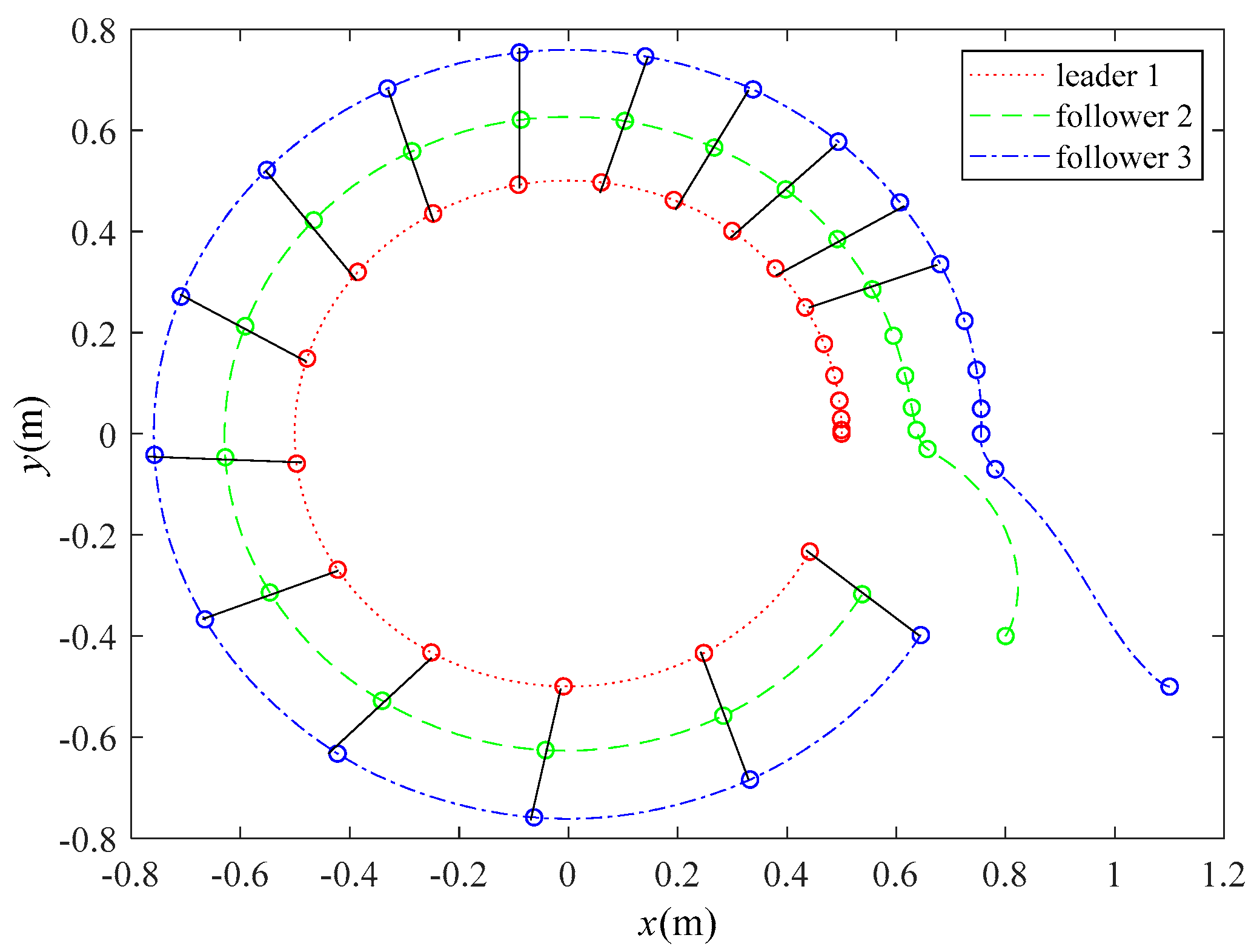
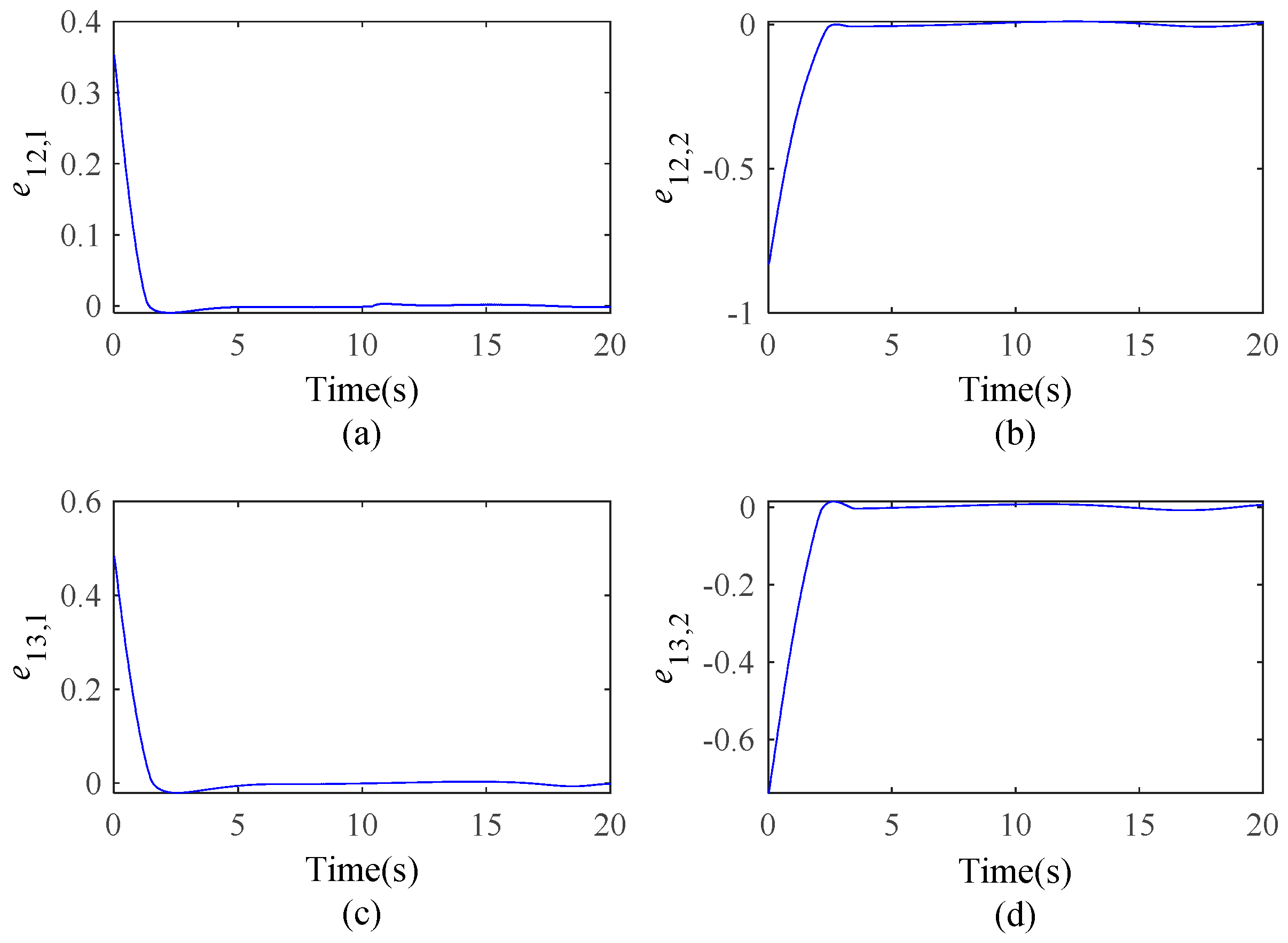
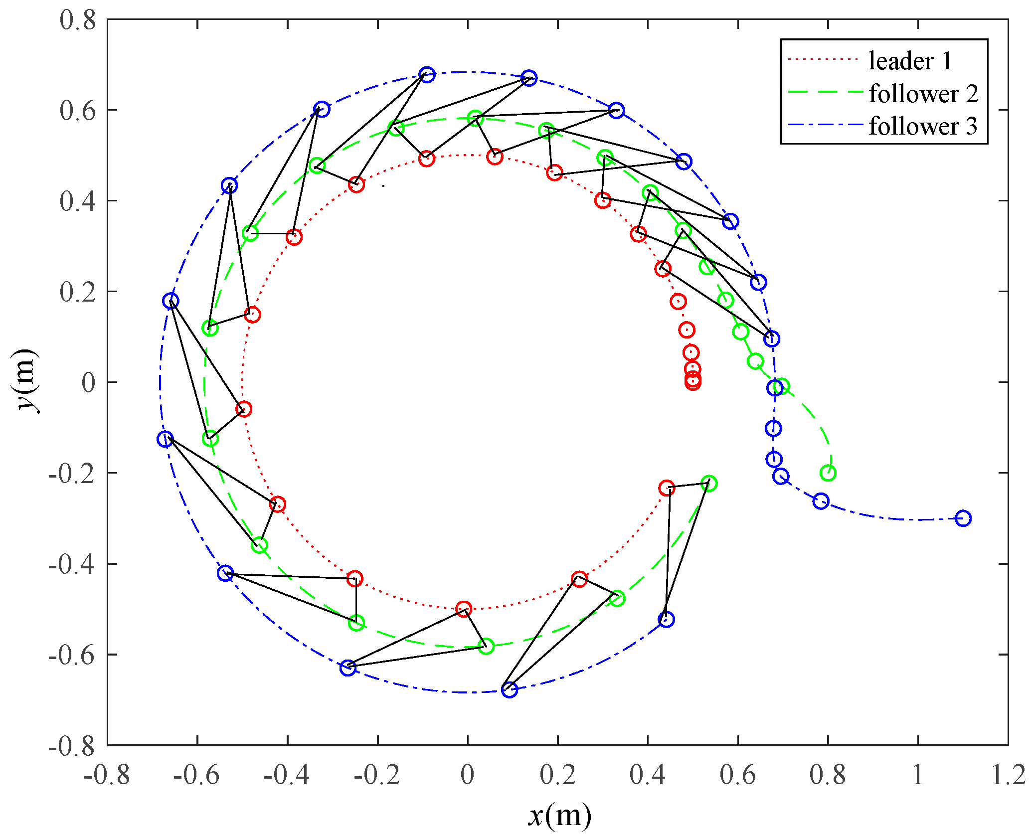
4.2.1. String Formation Moving Along a Circular Trajectory

In Figure 4, the multirobot platform carries out the task of string formation when moving along a circular trajectory, where the red indicates the leader robot and the green and blue indicate the two followers. The initial positions of the three robots were

$$q_1=[{\begin{array}{ccc}0.5\mathrm{m}& 0\mathrm{m}& 0.5\pi \mathrm{rad}]\end{array}}^T,q_2={[\begin{array}{ccc}0.8\mathrm{m}& -0.4\mathrm{m}& 0\mathrm{rad}\end{array}]}^T,\mathrm{and}{q}_3=[{\begin{array}{ccc}1.1\mathrm{m}& -0.5\mathrm{m}& \pi \mathrm{rad}]\end{array}}^T.$$

(51)

According to the initial positions in Equation (51) and the formation task, the initial states of the formation dynamics Equation (8) could be calculated as

$$x_{12}(0)={[\begin{array}{cccc}0.48\mathrm{m}& 0\mathrm{m}/\mathrm{s}& 1.24\pi \mathrm{rad}& 0\mathrm{rad}/\mathrm{s}\end{array}]}^T,x_{13}(0)={[\begin{array}{cccc}0.74\mathrm{m}& 0\mathrm{m}/\mathrm{s}& 1.26\pi \mathrm{rad}& 0\mathrm{rad}/\mathrm{s}\end{array}]}^T.$$

(52)

With regard to the formation task, the desired states could be determined as

$$x_{12}^d={[\begin{array}{cccc}0.13\mathrm{m}& 0\mathrm{m}/\mathrm{s}& -0.5\pi \mathrm{rad}& 0\mathrm{rad}/\mathrm{s}\end{array}]}^T,x_{13}^d={[\begin{array}{cccc}0.26\mathrm{m}& 0\mathrm{m}/\mathrm{s}& -0.5\pi \mathrm{rad}& 0\mathrm{rad}/\mathrm{s}\end{array}]}^T.$$

(53)

Figure 5 demonstrates the state variables when the multirobot system fulfilled the formation task in Figure 4. For the purpose of comparison, two other classic control methods were implemented on the same platform to accomplish the same formation task along with the presented super-twisting sliding mode control (STW) with ELM (abbreviated STW with ELM in Figure 5). These control methods were sliding mode control (SMC) with a disturbance observer (NDOBC) [18] (abbreviated SMC with NDOBC in Figure 5) and super-twisting sliding mode control (STW) alone, without ELM (abbreviated STW in Figure 5).

From Figure 5, the presented method can improve the performance of the system state variables. Note that the super-twisting sliding mode control on its own was performed with the same sliding surfaces formulated by Equation (11). Because of this, the ELM can improve the control performance. Furthermore, the control inputs of the three control methods applied to Follower 2 and Follower 3 are illustrated in Figure 6 and Figure 7, respectively.

As shown in Figure 6 and Figure 7, the presented method was able to effectively decrease the chattering phenomenon. In theory, the integrated method can completely compensate the disturbances and uncertainties entering the formation control system with increasing number of hidden layer nodes. However, the number of hidden layer nodes affects the computational burden.

Figure 8 illustrates the sliding surfaces. The estimations of uncertainties and the estimation errors are illustrated in Figure 9 and Figure 10. As proven in Theorem 1, the formation control system is asymptotically stable. From Figure 10, we know the errors are large at the outset, but the errors are dramatically decreased when the weights of the ELM are adjusted by (38).

4.2.2. Triangular Formation Moving in a Circular Trajectory

Figure 11 shows this platform forming a triangle when moving along a circular trajectory. Both the super-twisting sliding mode control parameters and the ELM parameters were kept unchanged. They were the same as in the formation task in Figure 4. Concerning this task, the initial positions of the three robots were set to

$$q_1=[{\begin{array}{ccc}0.5\mathrm{m}& 0\mathrm{m}& 0.5\pi \mathrm{rad}]\end{array}}^T,q_2={[\begin{array}{ccc}0.8\mathrm{m}& -0.2\mathrm{m}& \frac{1}{3}\pi \mathrm{rad}\end{array}]}^T,q_3=[{\begin{array}{ccc}1.1\mathrm{m}& -0.3\mathrm{m}& \pi \mathrm{rad}]\end{array}}^T.$$

(54)

According to this control task and the initial positions, the initial states of the formation dynamics could be calculated as

$$x_{12}(0)={[\begin{array}{cccc}0.36\mathrm{m}& 0\mathrm{m}/\mathrm{s}& 1.36\pi \mathrm{rad}& 0\mathrm{rad}/\mathrm{s}\end{array}]}^T,x_{13}(0)={[\begin{array}{cccc}0.63\mathrm{m}& 0\mathrm{m}/\mathrm{s}& 1.34\pi \mathrm{rad}& 0\mathrm{rad}/\mathrm{s}\end{array}]}^T.$$

(55)

Similarly, the desired states could be acquired on account of the leader’s trajectory.

$$x_{12}^d={[\begin{array}{cccc}0.13\mathrm{m}& 0\mathrm{m}/\mathrm{s}& 1.8\pi \mathrm{rad}& 0\mathrm{rad}/\mathrm{s}\end{array}]}^T,x_{13}^d={[\begin{array}{cccc}0.26\mathrm{m}& 0\mathrm{m}/\mathrm{s}& 1.2\pi \mathrm{rad}& 0\mathrm{rad}/\mathrm{s}\end{array}]}^T$$

(56)

The state variables and the control inputs were also similar to those in the formation task in Figure 4, as proven in Theorem 1, so these curves are not demonstrated due to the limited space.

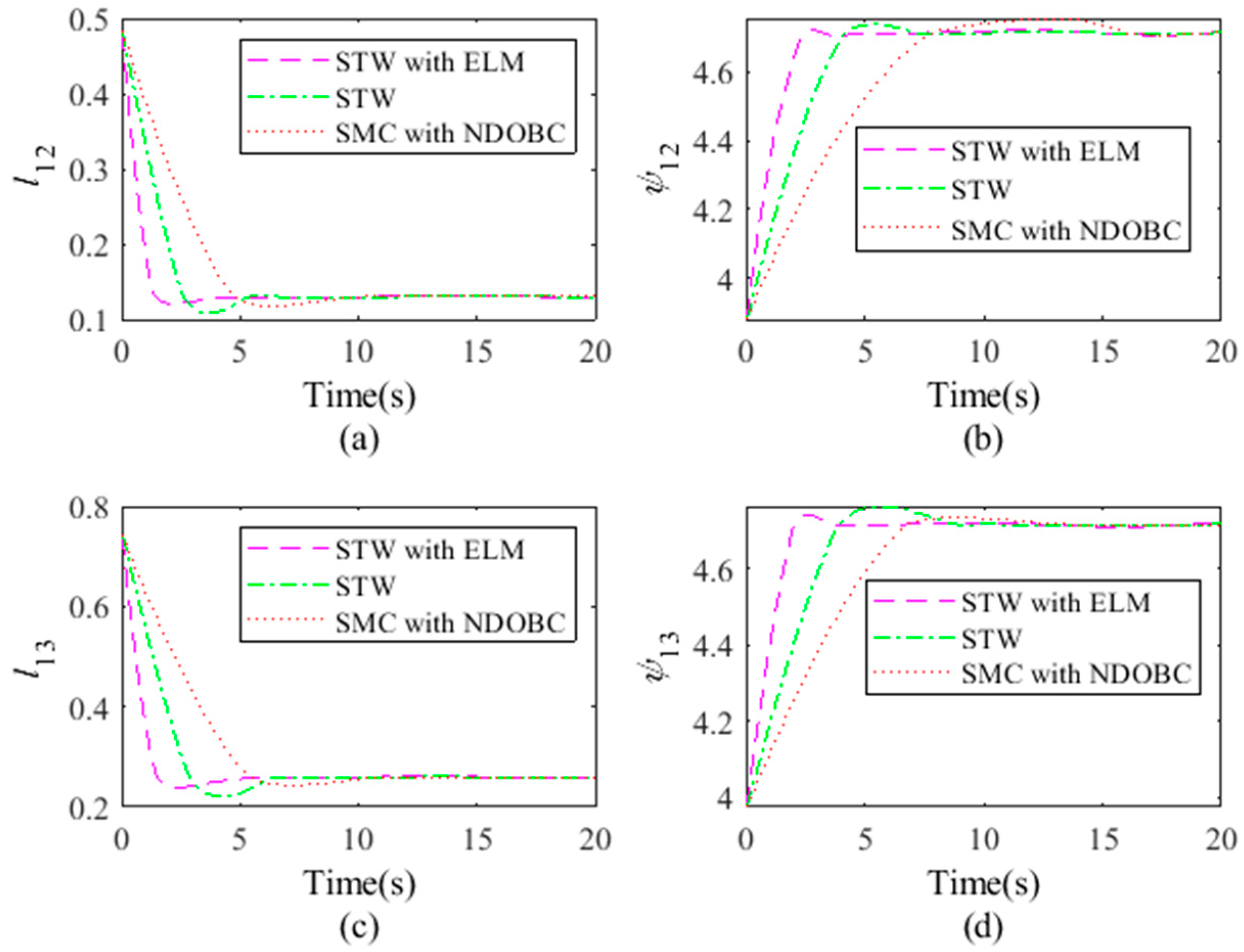
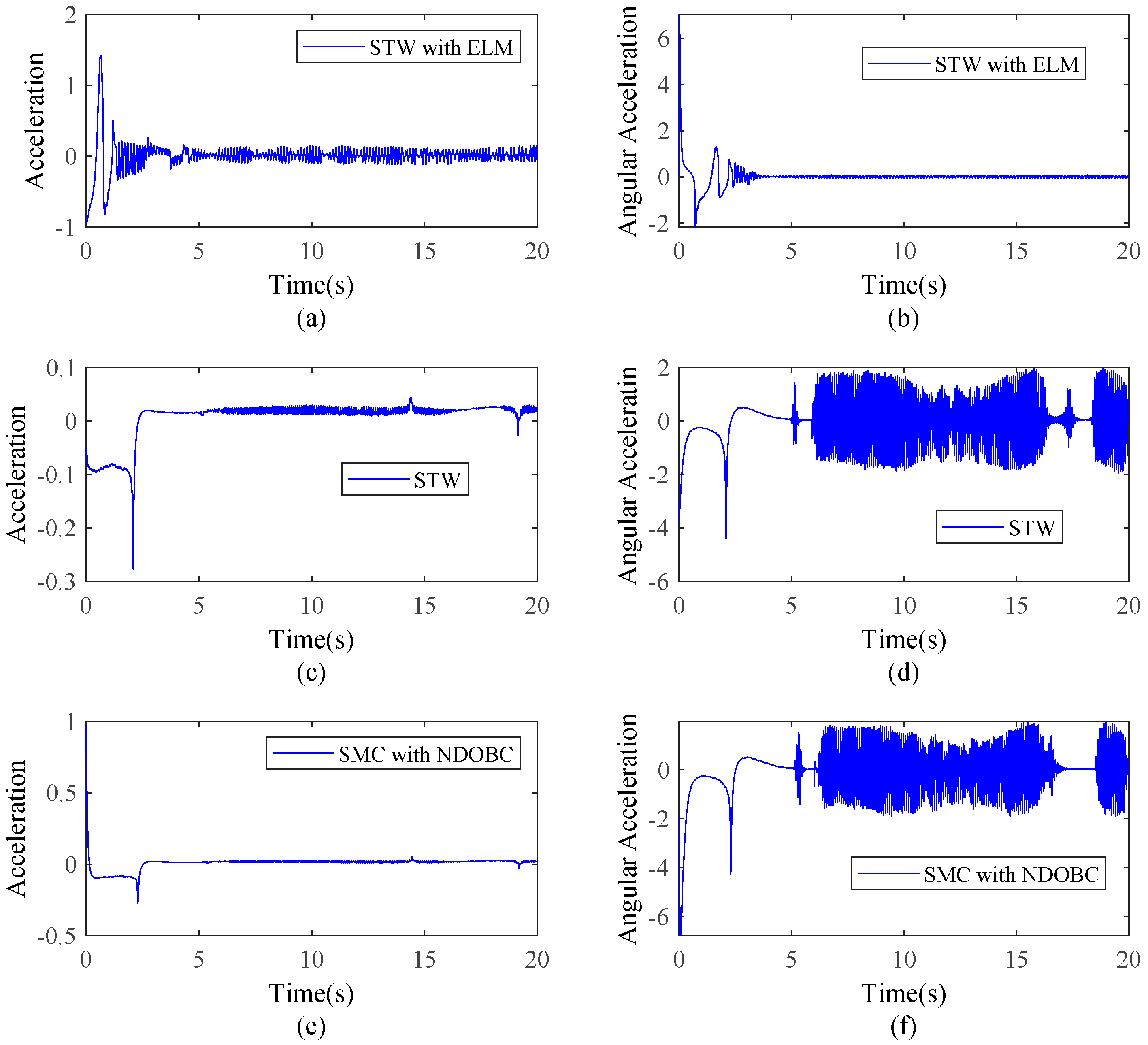
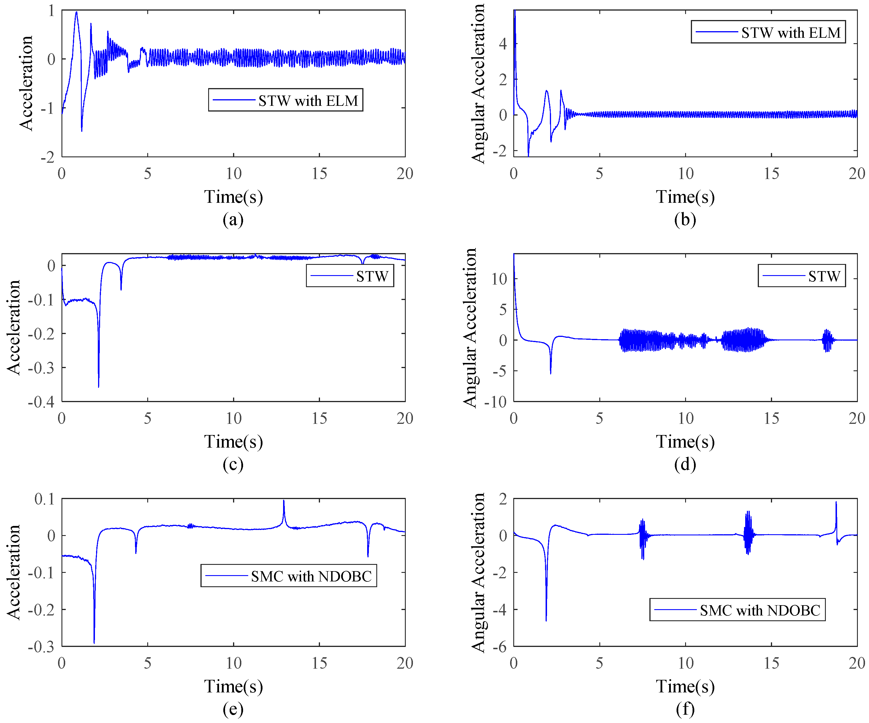
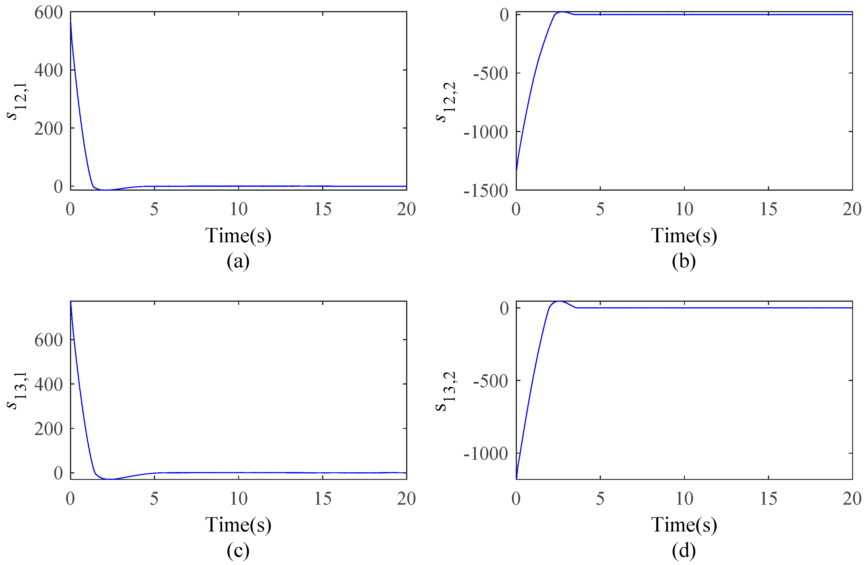
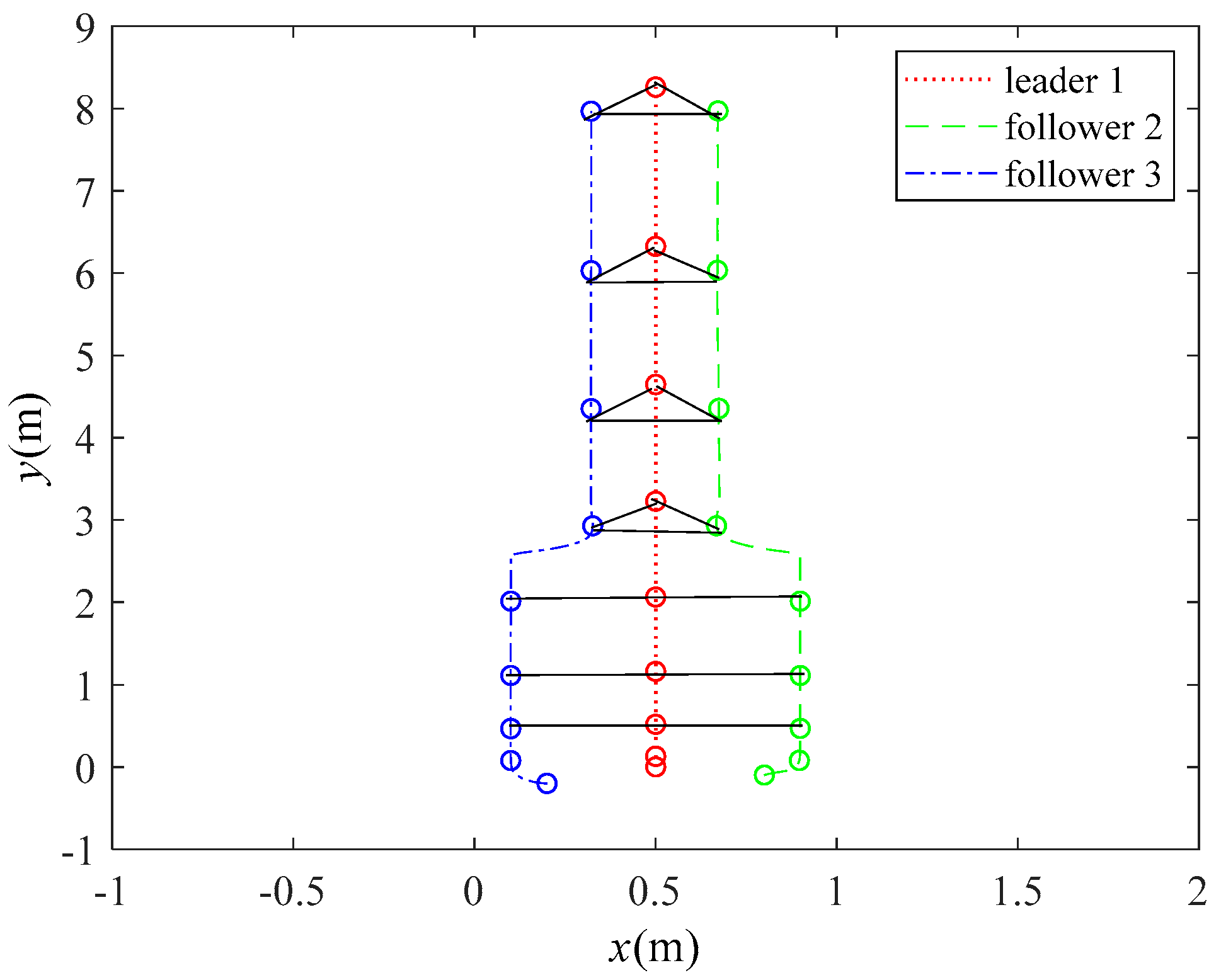
4.2.3. Maneuvers from a String Formation to a Triangular One

Firstly, Figure 12 shows the platform forming up into a string pattern when moving along a straight line. Then, the formation maneuvers to a triangular pattern. Both the super-twisting sliding mode control parameters and the ELM parameters were kept unchanged. They were the same as in the formation task in Figure 4.

Concerning this task, the initial positions of the three robots were set to

$$q_1=[{\begin{array}{ccc}0.5\mathrm{m}& 0\mathrm{m}& 0.5\pi \mathrm{rad}]\end{array}}^T,q_2={[\begin{array}{ccc}0.8\mathrm{m}& -0.1\mathrm{m}& \frac{1}{3}\pi \mathrm{rad}\end{array}]}^T,q_3=[{\begin{array}{ccc}0.2\mathrm{m}& -0.2\mathrm{m}& \pi \mathrm{rad}]\end{array}}^T.$$

(57)

According to the control task and the initial positions, the initial states of the formation dynamics could be calculated as

$$x_{12}(0)={[\begin{array}{cccc}0.33\mathrm{m}& 0\mathrm{m}/\mathrm{s}& 4.54\pi \mathrm{rad}& 0\mathrm{rad}/\mathrm{s}\end{array}]}^T,x_{13}(0)={[\begin{array}{cccc}0.40\mathrm{m}& 0\mathrm{m}/\mathrm{s}& 2.09\pi \mathrm{rad}& 0\mathrm{rad}/\mathrm{s}\end{array}]}^T.$$

(58)

The desired states could be acquired on account of the leader’s trajectory. When $0\le t<18\mathrm{s}$, the desired states of the string pattern were

$$x_{12}^d={[\begin{array}{cccc}0.4\mathrm{m}& 0\mathrm{m}/\mathrm{s}& 1.5\pi \mathrm{rad}& 0\mathrm{rad}/\mathrm{s}\end{array}]}^T,x_{13}^d={[\begin{array}{cccc}0.4\mathrm{m}& 0\mathrm{m}/\mathrm{s}& 0.5\pi \mathrm{rad}& 0\mathrm{rad}/\mathrm{s}\end{array}]}^T,$$

(59)

and when $18\mathrm{s}\le t<32\mathrm{s}$, the desired states of the triangular pattern were

$$x_{12}^d={[\begin{array}{cccc}0.3\mathrm{m}& 0\mathrm{m}/\mathrm{s}& 1.2\pi \mathrm{rad}& 0\mathrm{rad}/\mathrm{s}\end{array}]}^T$$

(60)

The state variables and the control inputs were also convergent, as proven in Theorem 1, so these curves are not demonstrated due to the limited space.

5. Conclusions

In this paper, we concentrated on the formation control of multirobot systems. In order to accomplish the formation task despite the inevitable uncertainties and disturbances, the super-twisting sliding mode control method was adopted. To deal with overestimation of the control gains, an ELM was constructed. The weights of the ELM between the hidden and output layers were adaptively adjusted. Theoretically, integration of the super-twisting sliding mode control and ELM for formation maneuvers has guaranteed stability in the sense of Lyapunov. The integrated method was applied to a multirobot platform with three mobile robots. Some comparisons were illustrated with two other control methods, that is, sliding mode control with a disturbance observer and super-twisting sliding mode control alone. Although all the three methods were able to fulfill the formation tasks, the numerical results illustrate that the integrated method had the best performance. This integrated method can be a solid support in dealing with the formation maneuvers of multiple uncertain robots.

References

- Ren, W.; Sorensen, N. Distributed coordination architecture for multi-robot formation control. Robot. Auton. Syst. 2008, 56, 324–333. [Google Scholar] [CrossRef]
- Dai, Y.Y.; Qian, D.W.; Lee, S. Multiple robots motion control to transport an object. Filomat 2018, 32, 1547–1558. [Google Scholar] [CrossRef]
- Chu, P.M.; Cho, S.; Fong, S.; Park, Y.W.; Cho, K. 3D Reconstruction framework for multiple remote robots on cloud system. Symmetry 2017, 9, 55. [Google Scholar] [CrossRef]
- Qian, D.W.; Xi, Y.F. Leader-Follower formation maneuvers for multi-robot systems via derivative and integral terminal sliding mode. Appl. Sci. 2018, 8, 1045. [Google Scholar] [CrossRef]
- Qian, D.W.; Zhang, G.G.; Chen, J.R.; Wang, J.; Wu, Z.M. Coordinated formation design of multi-robot systems via an adaptive-gain super-twisting sliding mode method. Appl. Sci. 2019, 9, 4315. [Google Scholar] [CrossRef]
- Yoo, S.J.; Park, B.S. Connectivity preservation and collision avoidance in networked nonholonomic multi-robot formation systems: Unified error transformation strategy. Automatica 2019, 103, 274–281. [Google Scholar] [CrossRef]
- Qian, D.W.; Tong, S.W.; Li, C.D. Observer-based leader-following formation control of uncertain multiple agents by integral sliding mode. Bull. Pol. Acad. Sci. Tech. Sci. 2017, 65, 35–44. [Google Scholar] [CrossRef]
- Qian, D.W.; Tong, S.W.; Guo, J.R.; Lee, S.G. Leader-follower-based formation control of non-holonomic mobile robots with mismatched uncertainties via integral sliding mode. Proc. Inst. Mech. Eng. Part I J. Syst. Control Eng. 2015, 229, 559–569. [Google Scholar] [CrossRef]
- Yao, X.Y.; Ding, H.F.; Ge, M.F. Formation-containment control for multi-robot systems with two-layer leaders via hierarchical controller-estimator algorithms. J. Frankl. Inst. Eng. Appl. Math. 2018, 355, 5272–5290. [Google Scholar] [CrossRef]
- Park, M.J.; Kwon, O.M.; Ryu, J.H. A Katz-centrality-based protocol design for leader-following formation of discrete-time multi-agent systems with communication delays. J. Frankl. Inst. 2018, 355, 6111–6131. [Google Scholar] [CrossRef]
- Sun, N.; Wu, Y.; Chen, H.; Fang, Y. Antiswing cargo transportation of underactuated tower crane systems by a nonlinear controller embedded with an integral term. IEEE Trans. Autom. Sci. Eng. 2019, 16, 1387–1398. [Google Scholar] [CrossRef]
- Qian, D.W.; Tong, S.W.; Lee, S.G. Fuzzy-Logic-based control of payloads subjected to double-pendulum motion in overhead cranes. Autom. Constr. 2016, 65, 133–143. [Google Scholar] [CrossRef]
- Liu, Y.; Jia, Y.M. Robust formation control of discrete-time multi-agent systems by iterative learning approach. Int. J. Syst. Sci. 2015, 46, 625–633. [Google Scholar] [CrossRef]
- Jin, X. Nonrepetitive leader-follower formation tracking for multiagent systems with LOS range and angle constraints using iterative learning control. IEEE Trans. Cybern. 2019, 49, 1748–1758. [Google Scholar] [CrossRef] [PubMed]
- Nascimento, T.P.; Conceicao, A.G.S.; Moreira, A.P. Multi-Robot nonlinear model predictive formation control: The obstacle avoidance problem. Robotica 2016, 34, 549–567. [Google Scholar] [CrossRef]
- Li, C.D.; Yi, J.Q.; Wang, H.K.; Zhang, G.Q.; Li, J.Q. Interval data driven construction of shadowed sets with application to linguistic word modeling. Inf. Sci. 2020, 507, 503–521. [Google Scholar] [CrossRef]
- Li, C.D.; Gao, J.L.; Yi, J.Q.; Zhang, G.Q. Analysis and design of functionally weighted single-input-rule-modules connected fuzzy inference systems. IEEE Trans. Fuzzy Syst. 2018, 26, 56–71. [Google Scholar] [CrossRef]
- Qian, D.W.; Tong, S.W.; Li, C.D. Leader-following formation control of multiple robots with uncertainties through sliding mode and nonlinear disturbance observer. ETRI J. 2016, 38, 1008–1018. [Google Scholar] [CrossRef]
- Qian, D.W.; Li, C.D.; Lee, S.G.; Ma, C. Robust formation maneuvers through sliding mode for multi-agent systems with uncertainties. IEEE CAA J. Autom. Sin. 2018, 5, 342–351. [Google Scholar] [CrossRef]
- Nair, R.R.; Karki, H.; Shukla, A.; Behera, L.; Jamshidi, M. Fault-Tolerant formation control of nonholonomic robots using fast adaptive gain nonsingular terminal sliding mode control. IEEE Syst. J. 2018, 13, 1006–1017. [Google Scholar] [CrossRef]
- Utkin, V.I. Discussion aspects of high-order sliding mode control. IEEE Trans. Autom. Control. 2016, 61, 829–833. [Google Scholar] [CrossRef]
- Uppal, A.A.; Alsmadi, Y.M.; Utkin, V.I.; Bhatti, A.I.; Khan, S.A. Sliding mode control of underground coal gasification energy conversion process. IEEE Trans. Control Syst. Technol. 2018, 26, 587–598. [Google Scholar] [CrossRef]
- Utkin, V.I.; Poznyak, A.S. Adaptive sliding mode control with application to super-twist algorithm: Equivalent control method. Automatica 2013, 49, 39–47. [Google Scholar] [CrossRef]
- Tian, C.; Li, C.D.; Zhang, G.; Lv, Y.S. Data driven parallel prediction of building energy consumption using generative adversarial nets. Energy Build. 2019, 186, 230–243. [Google Scholar] [CrossRef]
- Yang, Q.M.; Ge, S.S.; Sun, Y.X. Adaptive actuator fault tolerant control for uncertain nonlinear systems with multiple actuators. Automatica 2015, 60, 92–99. [Google Scholar] [CrossRef]
- Peng, W.; Li, C.D.; Zhang, G.; Yi, J.Q. Interval type-2 fuzzy logic based transmission power allocation strategy for lifetime maximization of WSNs. Eng. Appl. Artif. Intell. 2020. [Google Scholar] [CrossRef]
- Huang, G.B.; Wang, D.H.; Lan, Y. Extreme learning machines: A survey. Int. J. Mach. Learn. Cybern. 2011, 2, 107–122. [Google Scholar] [CrossRef]
- Wu, S.B.; Cao, W.H. Parametric model for microwave filter by using multiple hidden layer output matrix extreme learning machine. IET Microw. Antennas Propag. 2019, 13, 1889–1896. [Google Scholar] [CrossRef]
- Yu, Y.L.; Xu, M.X.; Gu, J. Vision-based traffic accident detection using sparse spatio-temporal features and weighted extreme learning machine. IET Intell. Transp. Syst. 2019, 13, 1417–1428. [Google Scholar] [CrossRef]
- Wong, P.K.; Gao, X.H.; Wong, K.I.; Vong, C.M.; Yang, Z.X. Initial-training-free online sequential extreme learning machine based adaptive engine air-fuel ratio control. Int. J. Mach. Learn. Cybern. 2019, 10, 2245–2256. [Google Scholar] [CrossRef]
© 2019 by the authors. Licensee MDPI, Basel, Switzerland. This article is an open access article distributed under the terms and conditions of the Creative Commons Attribution (CC BY) license (http://creativecommons.org/licenses/by/4.0/).
Share and Cite
Qian, D.; Zhang, G.; Wang, J.; Wu, Z. Second-Order Sliding Mode Formation Control of Multiple Robots by Extreme Learning Machine. Symmetry 2019, 11, 1444. https://doi.org/10.3390/sym11121444
Qian D, Zhang G, Wang J, Wu Z. Second-Order Sliding Mode Formation Control of Multiple Robots by Extreme Learning Machine. Symmetry. 2019; 11(12):1444. https://doi.org/10.3390/sym11121444
Chicago/Turabian StyleQian, Dianwei, Guigang Zhang, Jian Wang, and Zhimin Wu. 2019. "Second-Order Sliding Mode Formation Control of Multiple Robots by Extreme Learning Machine" Symmetry 11, no. 12: 1444. https://doi.org/10.3390/sym11121444
APA StyleQian, D., Zhang, G., Wang, J., & Wu, Z. (2019). Second-Order Sliding Mode Formation Control of Multiple Robots by Extreme Learning Machine. Symmetry, 11(12), 1444. https://doi.org/10.3390/sym11121444