Exact Solutions and Numerical Simulation of the Discrete Sawada–Kotera Equation

Abstract

We investigated an integrable five-point differential-difference equation called the discrete Sawada–Kotera equation. On the basis of the geometric series method, a new exact soliton-like solution of the equation is obtained that propagates with positive or negative phase velocity. In terms of the Jacobi elliptic function, a class of new exact periodic solutions is constructed, in particular stationary ones. Using an exponential generating function for Catalan numbers, Cauchy’s problem with the initial condition in the form of a step is solved. As a result of numerical simulation, the elasticity of the interaction of exact localized solutions is established.

1. Introduction

The theory of integrable differential-difference equations (DDE), based on the study of symmetries, conservation laws and recursion operators, is actively developing at present. As in the continuous case, the integrability of an equation is understood in the sense of the existence of Lax pairs or the infinite hierarchy of symmetries [1]. The theoretical results obtained in this direction are of great practical importance, since “models of a wide range of physical processes are inherently discrete” [2,3]. Most often, nonlinear models of physical processes allow analytical research only on the basis of the continuum limit of the initial discrete equation [4]. This is due to the fact that the construction of exact solutions of nonlinear DDEs other than the Toda, Volterra and Ablowitz–Ladik lattices is difficult [5].

Most integrable lattices have the Korteweg–de Vries and nonlinear Schrodinger equations as a continuum limit [6,7]. Recently, as a result of the classification of five-point DDEs [8], integrable discretizations of the Sawada–Kotera and Kaup–Kupershmidt equations have been identified.

The aim of this work is to conduct a qualitative study and numerical simulation of the integrable five-point discrete Sawada–Kotera equation

$$\frac{d}{dt}{u}_n\left(t\right)={\left[u_n\left(t\right)\right]}^2\left[u_{n+2}\left(t\right)u_{n+1}\left(t\right)-u_{n-1}\left(t\right)u_{n-2}\left(t\right)\right]-u_n\left(t\right)\left[u_{n+1}\left(t\right)-u_{n-1}\left(t\right)\right].$$

(1)

The considered DDE (1) is a linear combination of two famous integrable equations, the Volterra chain and the Ito–Narita–Bogoyavlensky chain [9,10,11], each of which has the Korteweg–de Vries equation as a continuous limit. It is known [12] that as these chains belong to different hierarchies, the flows corresponding to them do not commute, so the integrability of their linear combination is a nontrivial fact, which is established by constructing the corresponding Lax pair. It was shown in [12] that the introduction of new variables,

$$u_n=u(n,t)=\frac{1}{3}+\frac{{\epsilon }^2}{9}U(\epsilon n-\frac{4}{9}\epsilon t,\tau +\frac{2{\epsilon }^5}{135}t),$$

allows one to obtain the integrable Sawada–Kotera equation [13]

$$U_{\tau }=U_{xxxxx}+5U{U}_{xxx}+5U_x{U}_{xx}+5U^2{U}_x$$

from Equation (1) in the continuous limit for $\epsilon \to 0$. Therefore, Equation (1) is called the discrete Sawada–Kotera equation [14,15].

In [14], the general structure of the N-soliton solution of Equation (1) is given in terms of the Pfaffians. However, in specific cases of modeling processes of a discrete nature, information on the explicit form of physically realizable exact solutions is especially important for a researcher. Therefore, to achieve this goal, we solve several independent problems: The construction of exact solitary-wave and periodic solutions, the initial problem, and a numerical simulation of the obtained solutions.

The rest of the article is structured as follows. In the next two sections, an exact solitary-wave solution and a periodic solution will be constructed. In the fourth section, some combinatorial dependencies will be established when solving an initial value problem for Equation (1). In the fifth section, exact stationary solutions are discussed, and in the last section, numerical simulations are performed that demonstrate the stability of exact localized solutions and the elasticity of their interaction.

2. Solitary Wave Solution

Let us find an exact solitary-wave solution to the Equation (1). In [16,17], algorithms were developed for computer mathematics systems and exact kink-like solutions were obtained for Toda, Volterra, and Ablowitz–Ladik lattices and their generalizations. To construct an exact localized solution, we will use a modification of the geometric series method [18]. In the continuous case, this approach allows one to obtain exact soliton-like solutions of integrable and non-integrable equations with a polynomial dispersion relation as the sum of the geometric series of the perturbation method in powers of exponential function.

The transition to the traveling wave variable $z=dn+\omega t$ allows us to write Equation (1) as follows

$$-\omega \frac{d}{dz}u(z)+{\left[u(z)\right]}^2\left[u(z+2d)u(z+d)-u(z-d)u(z-2d)\right]-u(z)\left[u(z+d)-u(z-d)\right]=0.$$

(2)

After substituting in Equation (2) a functional series with unknown coefficients $C_k$

$$u(z)=\sum _{k=0}^{\infty }{C}_k{\mathrm{e}}^{kz},$$

(3)

$$u(z+md)=\sum _{k=0}^{\infty }{C}_k{\mathrm{e}}^{k\left(z+md\right)}=\sum _{k=0}^{\infty }{C}_k{\delta }^{km}{\mathrm{e}}^{kz},$$

(4)

where $m=\pm 1,\pm 2,$ $\delta ={\mathrm{e}}^d$, we group the terms in powers of the exponential function. In the lower order, at ${\mathrm{e}}^z$, we obtain a “linear dispersion relation” for determining the frequency $\omega$:

$$\omega =C_0\left(1-{\delta }^{-2}\right)\left[C_0^2\left({\delta }^2+1\right)+\left(C_0^2-1\right)\delta \right].$$

(5)

Successively equating to zero the coefficients at ${\mathrm{e}}^{2z},{\mathrm{e}}^{3z},\dots$, we calculate $C_2,C_3,\dots$:

$$\begin{array}{c}{C}_2=-{\displaystyle \frac{\delta C_1^2}{C_0{\left(\delta -1\right)}^2}},C_3={\displaystyle \frac{C_1^3{\delta }^2\left({\delta }^2+\delta +1\right)}{C_0^2{\left(\delta -1\right)}^4{\left(\delta +1\right)}^2}},\hfill \\ C_4=-{\displaystyle \frac{C_1^4{\delta }^3\left({\delta }^2+1\right)}{C_0^3{\left(\delta -1\right)}^6{\left(\delta +1\right)}^2}},C_5={\displaystyle \frac{C_1^5{\delta }^4\left({\delta }^4+{\delta }^3+{\delta }^2+\delta +1\right)}{C_0^4{\left(\delta -1\right)}^8{\left(\delta +1\right)}^4}},\hfill \\ C_6=-{\displaystyle \frac{C_1^6{\delta }^5\left({\delta }^4+{\delta }^2+1\right)}{C_0^5{\left(\delta -1\right)}^{10}{\left(\delta +1\right)}^4}},C_7={\displaystyle \frac{C_1^7{\delta }^6\left({\delta }^6+{\delta }^5+{\delta }^4+{\delta }^3+{\delta }^2+\delta +1\right)}{C_0^6{\left(\delta -1\right)}^{12}{\left(\delta +1\right)}^6}},\dots \hfill \end{array}$$

(6)

All coefficients, starting from $C_2$, are expressed through three arbitrary parameters $C_0$, $C_1$ and $\delta$. Looking at Equations (6), it is easy to write the general formula for the coefficient $C_n$; however, this is not necessary. The series (3) with coefficients (6) is a geometric series and its sum gives an exact solution to Equation (2). To verify this, we use the remarkable property of Padé approximants: Successive diagonal approximants $[1/1]$, $[2/2]$, $[3/3]$,…, calculated for an arbitrary geometric power series, coincide, starting from some order $[N/N]$.

Let us prove the presence of this property. As is known, the Padé approximant of order $\left[M/N\right]$ for power series $S(x)={\displaystyle \sum _k}{a}_k{x}^k$ is the ratio of polynomials

$$\left[M/N\right]=\frac{P_M(x)}{Q_N(x)}=\frac{p_0+p_{1}x+\dots +p_M{x}^M}{q_0+q_{1}x+\dots +q_N{x}^N},$$

(7)

whose Maclaurin series expansion $T_{M,N}(x)$ coincides with $S(x)$ as long as possible [19,20]. To calculate the coefficients $p_k,q_k$ of the ratio (7) we use the first $M+N+2$ terms of the series $S(x)$. Formal representation,

$$\frac{P_M(x)}{Q_N(x)}=\frac{P_M(x)}{1-\left(1-Q_N(x)\right)},$$

(8)

means that the Maclaurin series $T_{M,N}(x)$ for Equation (7) is a geometric series with the first term $P_M$ and the denominator $\left(1-Q_N\right)$, and the approximant (7) itself is the exact sum of its Maclaurin series. Suppose that for geometric series $T_{M,N}(x)$ we calculated a higher order approximant, for example, $\left[M+1/N+1\right]$. Obviously, its own Maclaurin series $T_{M+1,N+1}(x)$ is also geometric and its first $M+N+4$ terms coincide with the terms of $T_{M,N}(x)$. The geometric series can be continued in its first terms uniquely, therefore, the series $T_{M,N}(x)$ and $T_{M+1,N+1}(x)$ coincide and after them the approximants $\left[M/N\right]$ and $\left[M+1/N+1\right]$ coincide identically, as required.

Replacing ${\mathrm{e}}^z=Z$ in Equation (3), we begin to sequentially calculate for Equation (3) the diagonal Padé approximants, starting with $\left[1/1\right]$. It turns out that the second and third order approximants coincide:

$$\left[2/2\right]=\left[3/3\right]=C_0+\frac{C_{1}Z}{\left(1+{\displaystyle \frac{\delta C_{1}Z}{\left(\delta +1\right){\left(\delta -1\right)}^2{C}_0}}\right)\left(1+{\displaystyle \frac{{\delta }^2{C}_{1}Z}{\left(\delta +1\right){\left(\delta -1\right)}^2{C}_0}}\right)}.$$

(9)

Without calculating an approximant of higher order, we check whether Equation (9) gives an exact solution to the problem. Returning to variables $z,d$ in Equations (9) and (5) we obtain

$$u(z)=C_0\left(1+\frac{{\mathrm{e}}^{z+z_0}}{\left(1+A{\mathrm{e}}^{z+z_0}\right)\left(1+A{\mathrm{e}}^{z+z_0+d}\right)}\right),$$

(10)

$$\omega =C_0\left(1-{\mathrm{e}}^{-2d}\right)\left[C_0^2\left({\mathrm{e}}^{2d}+1\right)+\left(C_0^2-1\right){\mathrm{e}}^d\right],$$

(11)

where $A={\mathrm{e}}^d{\left({\mathrm{e}}^d+1\right)}^{-1}{\left({\mathrm{e}}^d-1\right)}^{-2}$, $z_0=\ln \left(C_1/\phantom{C_1{C}_0}{C}_0\right)$. Substitution of Equations (10) and (11) into Equation (2) turns the latter into identity, therefore, Equation (10) is an exact solution of Equation (2) under condition (11). After substitution $z=dn+\omega t$ expression (10) becomes a solitary-wave solution of the original Equation (1). The shape of this solution depends on the relationship between the parameters A and d and varies from a flat-peak pulse to a pulse with a sharp peak on the pedestal $C_0$ (Figure 1).

The number of lattice nodes per pulse width depends on the parameter d, playing the role of the wave number. The solution in Figure 1a corresponds to $d=1$ and visually about 15 nodes are located along the pulse width; for the solution in Figure 1b we have $d=12$ and only 2–3 nodes across the pulse width.

3. Periodic Solution

The leading terms balance gives a simple pole for solution of Equation (2). In accordance with the truncated expansion method [21], we will use the ansatz with the Jacobi elliptic function:

$$u(z)=A+B\mathrm{sn}(z,m).$$

(12)

Using the addition theorem for Jacobi elliptic functions, we have:

$$\begin{array}{c}u(z\pm d)=A-B\frac{CD\mathrm{sn}\left(z,m\right)\pm S\mathrm{cn}\left(z,m\right)\mathrm{dn}\left(z,m\right)}{m^2{S}^2{\mathrm{sn}}^2\left(z,m\right)-1},\hfill \\ u(z\pm 2d)=A-B\frac{C_2{D}_2\mathrm{sn}\left(z,m\right)\pm S_2\mathrm{cn}\left(z,m\right)\mathrm{dn}\left(z,m\right)}{m^2{S}_2^2{\mathrm{sn}}^2\left(z,m\right)-1},\hfill \end{array}$$

(13)

where

$$\begin{array}{c}S=\mathrm{sn}(d,m),C=\mathrm{cn}(d,m),D=\mathrm{dn}(d,m),\hfill \\ S_2=\mathrm{sn}(2d,m),C_2=\mathrm{cn}(2d,m),D_2=\mathrm{dn}(2d,m).\hfill \end{array}$$

(14)

The constants $S_2,C_2,D_2$ are expressed through $S,C,D$ by means of double argument formulas:

$$S_2=-\frac{2SCD}{S^4{m}^2-1},C_2=\frac{D^2{S}^2-C^2}{S^4{m}^2-1},D_2=\frac{C^2{S}^2{m}^2-D^2}{S^4{m}^2-1}.$$

(15)

Taking into account Equation (14), we substitute Equations (12) and (13) into Equation (2). After dividing by a common factor $4B\mathrm{cn}\left(z,m\right)\mathrm{dn}\left(z,m\right)$, the left-hand side of Equation (2) reduces to a fourth-order polynomial with respect to $\mathrm{sn}\left(z,m\right)$:

$$\sum _{n=0}^4{A}_n{\mathrm{sn}}^n\left(z,m\right)=0,$$

(16)

where

$$\begin{array}{c}{A}_0=\left[\left(2S{A}^3-2SA-\omega \right)\left(S^4{m}^2-1\right)-4SCD{A}^3\right]\left(S^4{m}^2-1\right),\hfill \\ A_1=2SB\left[\left(2S^8{m}^4-S^4{m}^2{\left(CD+2\right)}^2-S^2\left(C^4{m}^2+D^4\right)+\right.\right.\hfill \\ \left.\left.CD\left(3CD+4\right)+2\right)A^2-S^4{m}^2\left(S^4{m}^2-2\right)-1\right],\hfill \\ A_2=S\left[S^5{m}^4\omega \left(S^4{m}^2-2\right)+2A{B}^2{S}^8{m}^4+4A^3\right.m^4{S}^{6}CD-\hfill \\ 4A{B}^2{S}^4{m}^2\left(C^2{D}^2+CD+1\right)-4A{S}^2\left(A^{2}CD{m}^2\left(2CD+1\right)\right.+\hfill \\ \left.C^2{m}^2\left(B^2{C}^2-2D^2\right)+B^2{D}^4\right)+S{m}^2\omega \left(4C^2{D}^2+1\right)+\hfill \\ \left.2A{B}^2\left(6C^2{D}^2+2CD+1\right)\right],\hfill \\ A_3=2BS\left[4A^2{m}^{4}CD{S}^6-B^2{C}^2{D}^2\left(S^4{m}^2-3\right)-\right.\hfill \\ \left.S^2\left(m^2{B}^2{C}^4+4C^2{D}^2{m}^2\left(2A^2-1\right)+4A^2{m}^{2}CD+B^2{D}^4\right)\right],\hfill \\ A_4=4D{m}^{2}C{S}^3\left[A{B}^2\left(S^4{m}^2-1\right)-CD\left(S{m}^2\omega +2A{B}^2\right)\right].\hfill \end{array}$$

(17)

The system of nonlinear equations $\left\{A_n=0\right\},n=0\dots 4$, supplemented by the relations between Jacobi elliptic functions $\mathrm{cn}$, $\mathrm{sn}$ and $\mathrm{dn}$:

$$C^2+S^2=1,D^2+m^2{S}^2=1,$$

(18)

can be solved by any of the modern computer mathematics software systems, for example, Maple. The solution contains several branches corresponding to stationary waves $\left(\omega =0\right)$ and traveling waves $\left(\omega \ne 0\right)$. Two combinations of parameters correspond to traveling waves. The first of them has the form

$$\begin{array}{c}A=\pm \frac{1}{2},B=\pm \frac{1}{2}\sqrt{1-D^2},C=\frac{D}{1-D},S=\pm \frac{\sqrt{1-2D}}{1-D},\hfill \\ m=\pm \left(1-D\right)\sqrt{\frac{1-D^2}{1-2D}},\omega =\pm \frac{\sqrt{1-2D}}{2\left(1-D\right)},\hfill \end{array}$$

(19)

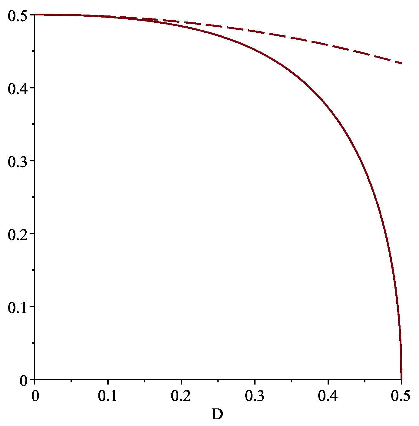
where all signs can be selected arbitrarily. The second combination is obtained from the first one by substitution $D\to -D$. Note that the solution Equation (12) at each moment of time is determined only on a uniform grid $nd+z_0$, $n\in Z$. If the ratio of the grid step d to the period T of function $\mathrm{sn}(z,m)$ is not a rational number, then the period of the grid function $u_n=A+B\mathrm{sn}(nd+z_0,m)$ tends to infinity and we obtain a non-periodic solution. It can be shown that function (12) under conditions (19) gives an exact periodic solution of Equation (1). This solution is real for $0<D<\frac{1}{2}$ and its period T has six nodes of the lattice for any admissible value of D. With an increase in parameter D frequency $\omega$ and amplitude B decrease monotonously (Figure 2).

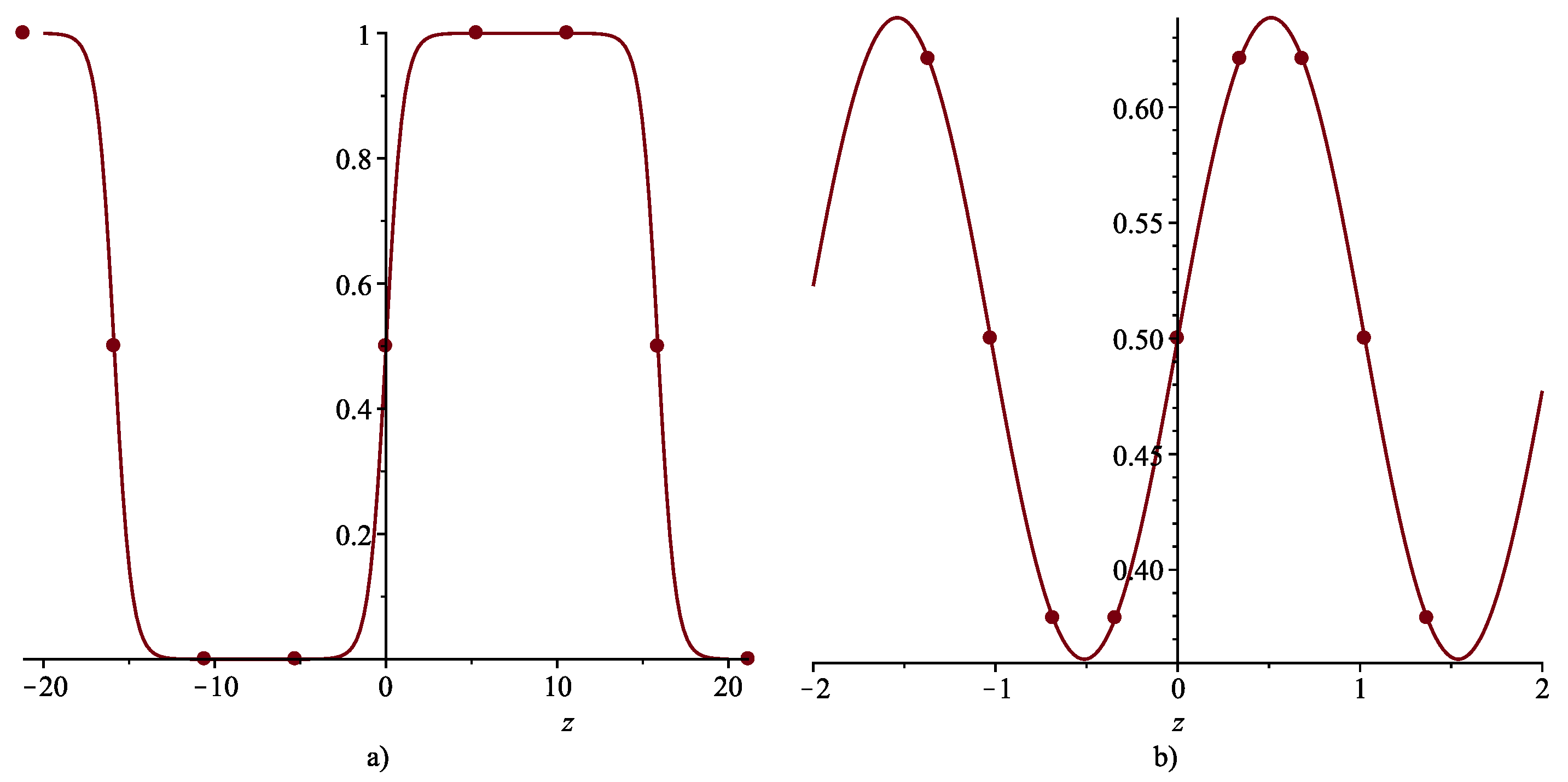
If we take into account that the intrinsic amplitude of function $\mathrm{sn}(z,m)$ when $\left|m\right|>1$ is $A_{sn}=\frac{1}{m}$, then the total oscillation amplitude $A_{sn}B$ of solution (12) turns out to be numerically the same as the frequency $\omega$. Examples of a traveling waveform are shown in Figure 3.

4. Exact Solution and Catalan Numbers

An interesting property of the modified Volterra lattice,

$$\frac{d}{dt}{u}_n(t)={\left[u_n(t)\right]}^2\left[u_{n+1}(t)-u_{n-1}(t)\right],$$

(20)

is revealed in articles [22,23]. It turns out that for a special initial condition,

$$u_0(0)=0,u_1(0)=u_2(0)=\dots =1,$$

(21)

we can write the exact solution of Equation (20) in closed form, and this solution is neither of periodic type, nor of traveling-wave type.

We apply the methodology [22,23] to the lattice Equation (1) with the same initial condition (21). First, note that $u_0(t)\equiv 0$. Due to this equality, Equation (1) with any positive number n are independent of the values of the grid function at nodes with negative numbers $u_{-1},u_{-2},\dots$. We will solve the initial problem Equations (1), (21) for positive nodes $u_1,u_2,\dots$

By sequentially differentiating both sides of Equation (1) with respect to t and replacing the first derivatives in the right-hand sides with the help of Equation (1), we can express any higher derivative $u_n^{(k)}(t)$ in terms of $u_p(t)$, for example,

$$\begin{array}{c}{\displaystyle \frac{d{u}_1}{dt}}=u_1{u}_2\left(u_1{u}_3-1\right),\hfill \\ {\displaystyle \frac{d^2{u}_1}{d{t}^2}}=u_1{u}_2\left[u_1^2{u}_3\left(u_2{u}_3+1\right)\right.-u_2{u}_3{u}_4+u_2+u_3-u_1+\hfill \\ \left.u_1{u}_3\left(u_3\left(u_2{u}_4+u_4{u}_5-1\right)-2u_2-u_4\right)\right],\dots \hfill \end{array}.$$

(22)

Substituting to Equation (22) the initial conditions (21), we obtain the sequence $u_n^{(0)}(0)$, $u_n^{(1)}(0)$, $u_n^{(2)}(0)$,... of initial values for the k-th derivatives for the n-th node of the lattice:

$$\begin{array}{c}n=1:1,0,0,0,0,0,0,0,\dots \hfill \\ n=2:1,1,2,5,14,42,132,429,\dots \hfill \\ n=3:1,0,0,0,0,0,0,0,\dots \hfill \\ n=4:1,0,-1,-2,2,28,65,-338,\dots \hfill \\ n=5:1,0,0,0,0,0,0,0,\dots \hfill \\ n=6:1,0,0,1,2,-3,-10,79,\dots \hfill \end{array}.$$

(23)

For odd nodes ($n=2p+1$) we observe that for $k>0$ the initial values of the derivatives $u_{2p+1}^{\left(k\right)}(0)$ are zero, at least for the first eight calculated values. It can be assumed that during the evolution of the system, the values at these nodes do not change:

$$u_{2p+1}^{}(t)=u_{2p+1}^{}(0)=1.$$

(24)

In fact, substituting Equation (24) into Equation (1) for an odd knot, we have

$$\begin{array}{c}\frac{d}{dt}{u}_{2p+1}(t)={\left[u_{2p+1}(t)\right]}^2\left[u_{2p+3}(t)u_{2n+2}(t)-u_{2p}(t)u_{2p-1}(t)\right]-\hfill \\ u_{2p+1}(t)\left[u_{2p+2}(t)-u_{2p}(t)\right]=u_{2n+2}(t)-u_{2p}(t)-\left[u_{2n+2}(t)-u_{2p}(t)\right]\equiv 0.\hfill \end{array}$$

(25)

For even nodes the situation is more complicated. For $n=2$ we have a sequence of Catalan numbers $c_n=\frac{(2n)!}{n!\left(n+1\right)!}$, for $n=4$ we get a sequence whose generating function is inverse to the generating function for Catalan numbers, and the sequence for $n=6$ is no longer recognized by Sloane’s online sequence encyclopedia [24]. We explicitly write Equation (1) for even nodes taking into account (24):

$$\begin{array}{c}\frac{d}{dt}{u}_{2p}(t)={\left[u_{2p}(t)\right]}^2\left[u_{2p+2}(t)u_{2p+1}(t)-u_{2p-1}(t)u_{2p-2}(t)\right]-\hfill \\ u_{2p}(t)\left[u_{2p+1}(t)-u_{2p-1}(t)\right]={\left[u_{2p}(t)\right]}^2\left[u_{2p+2}(t)-u_{2p-2}(t)\right].\hfill \end{array}$$

(26)

Obviously, Equations (26) coincide with (20) up to renumbering. In [22] it is shown that the exact solution of Equation (20) with the initial condition (21) is

$$u_n=\frac{w_{n-3}{w}_{n-1}}{w_{n-2}^2},n=1,2,\dots ,$$

(27)

where $w_{-2}=w_{-1}=1$ and, for $k\ge 0$,

$$w_{2k}=\left|\begin{array}{cccc}f& f^{\prime }& \dots & f^{\left(k\right)}\\ f^{\prime }& f^{″}& \dots & f^{\left(k+1\right)}\\ \dots & \dots & \dots & \dots \\ f^{\left(k\right)}& f^{\left(k+1\right)}& \dots & f^{\left(2k\right)}\end{array}\right|,w_{2k+1}=\left|\begin{array}{cccc}{f}^{\prime }& f^{″}& \dots & f^{\left(k+1\right)}\\ f^{″}& f^{‴}& \dots & f^{\left(k+2\right)}\\ \dots & \dots & \dots & \dots \\ f^{\left(k+1\right)}& f^{\left(k+2\right)}& \dots & f^{\left(2k+1\right)}\end{array}\right|.$$

(28)

In Equations (28) the notation $u_1=f(t)$ is taken. Thus, all unknown functions $u_2(t),u_3(t),\dots$ are expressed in closed form through function $u_1(t)$ and its derivatives ${u_1}^{\prime }(t),{u_1}^{″}(t),\dots$. You can find function $u_1(t)$ itself through the exponential generating function for the Catalan numbers $c_n$, which serve as the coefficients of the expansion of $u_1(t)$ in the Maclaurin series:

$$f(t)=\sum _{n=0}^{\infty }\frac{c_n}{n!}{t}^n={\mathrm{e}}^{2t}\left[I_0(2t)-{I_0}^{\prime }(2t)\right],$$

(29)

where $I_0(z)$ is the modified Bessel function, which is a solution to the Cauchy problem

$$z{I_0}^{″}(z)+{I_0}^{\prime }(z)-z{I}_0\left(z\right)=0,I_0(0)=1,{I_0}^{\prime }(0)=0.$$

(30)

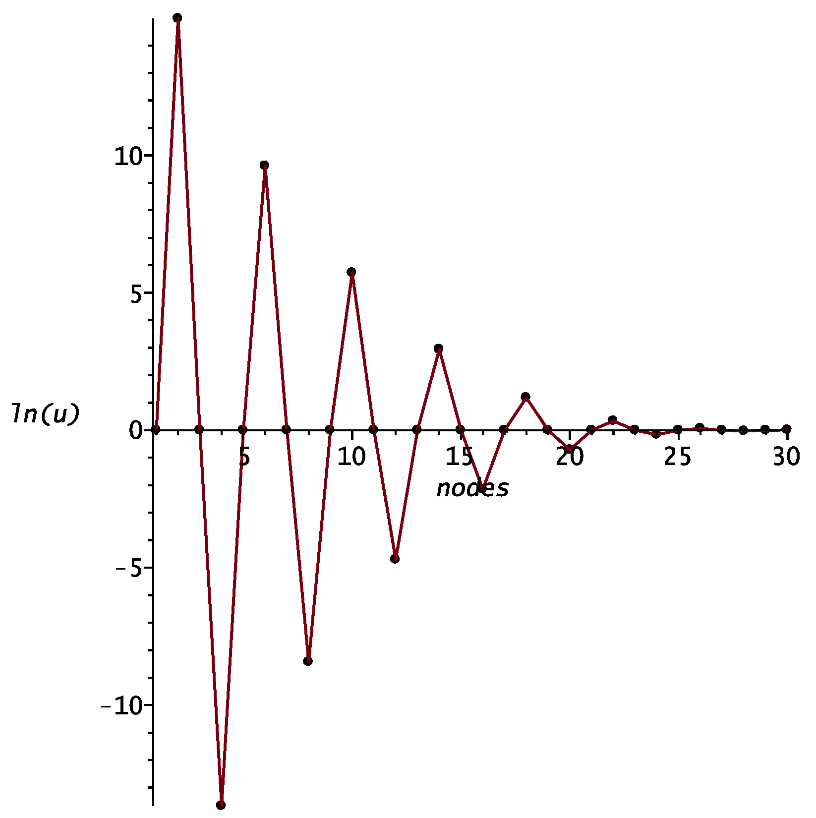
Unfortunately, the solutions of both the modified Volterra lattice Equation (20) and Equation (1) demonstrate an exponential increase in time and, therefore, are limited in physical applications (Figure 4). The behavior of the solution depends on the node number n: We have $u_n=1$ for $n=1,3,5,\dots$; $\underset{t\to \infty }{lim}{u}_n\left(t\right)=+\infty$ for $n=2,6,10,\dots$; $\underset{t\to \infty }{lim}{u}_n\left(t\right)=0$ for $n=4,8,12,\dots$.

5. Stationary Solutions

The simplest stationary (time-independent) solutions of Equation (1)—constant solution $u_n=const$ and sawtooth solution $u_{2n}=a,u_{2n+1}=b$—can be obtained by direct selection. Periodic stationary solutions $u_{n+kN}=a_n,n=1\dots N,k\in Z$, represented by a repeating set of N constants $\left\{a_1,a_2,\dots ,a_N\right\}$, are determined from the solution of the system,

$$a_{n+2}^2\left(a_{n+4}{a}_{n+3}-a_{n+1}{a}_n\right)-a_{n+2}\left(a_{n+3}-a_{n+1}\right)=0,a_{n+N}=a_n,n=1\dots N.$$

(31)

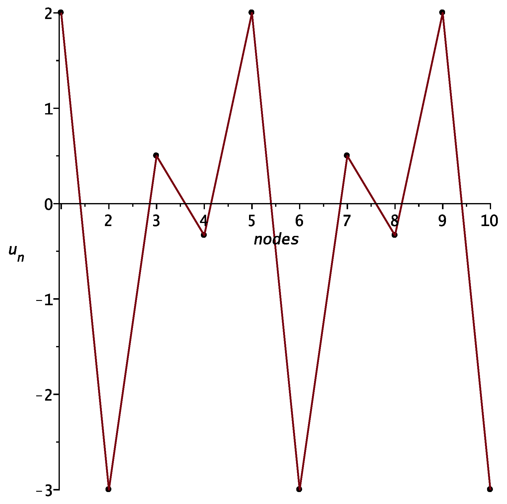
As N increases, the set of stationary solutions expands. For example, if for $N=3$ we have a unique solution of the form $\left\{0,0,a\right\}$, then for $N=4$ we find four solutions $\left\{0,a,0,b\right\}$, $\left\{1,a,1,b\right\}$, $\left\{-1,a,-1,b\right\}$ and $\left\{a,b,\frac{1}{a},\frac{1}{b}\right\}$. Note that the first three options for $N=4$ make it possible to construct non-periodic solutions, since the quantities a and b can be specified arbitrarily in each set of four numbers. The graph of the 4th option for $N=4$ at $a=2,b=-3$ is shown in Figure 5.

Another variant of the non-periodic stationary solution follows from Equation (10), where the constants $C_0$ and d should be selected from the condition that the frequency $\omega$ defined by Equation (11) vanishes.

6. Numerical Simulation

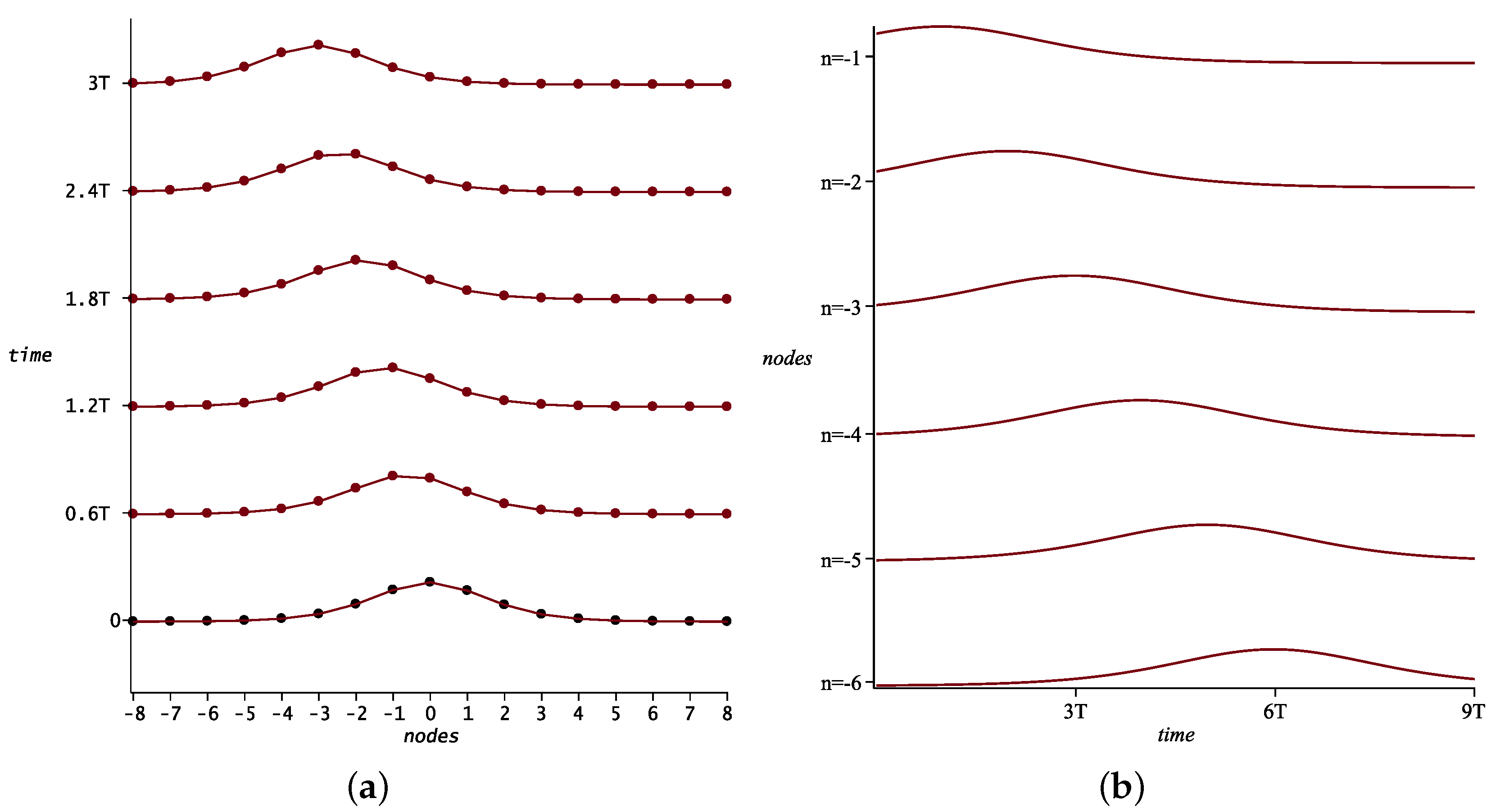
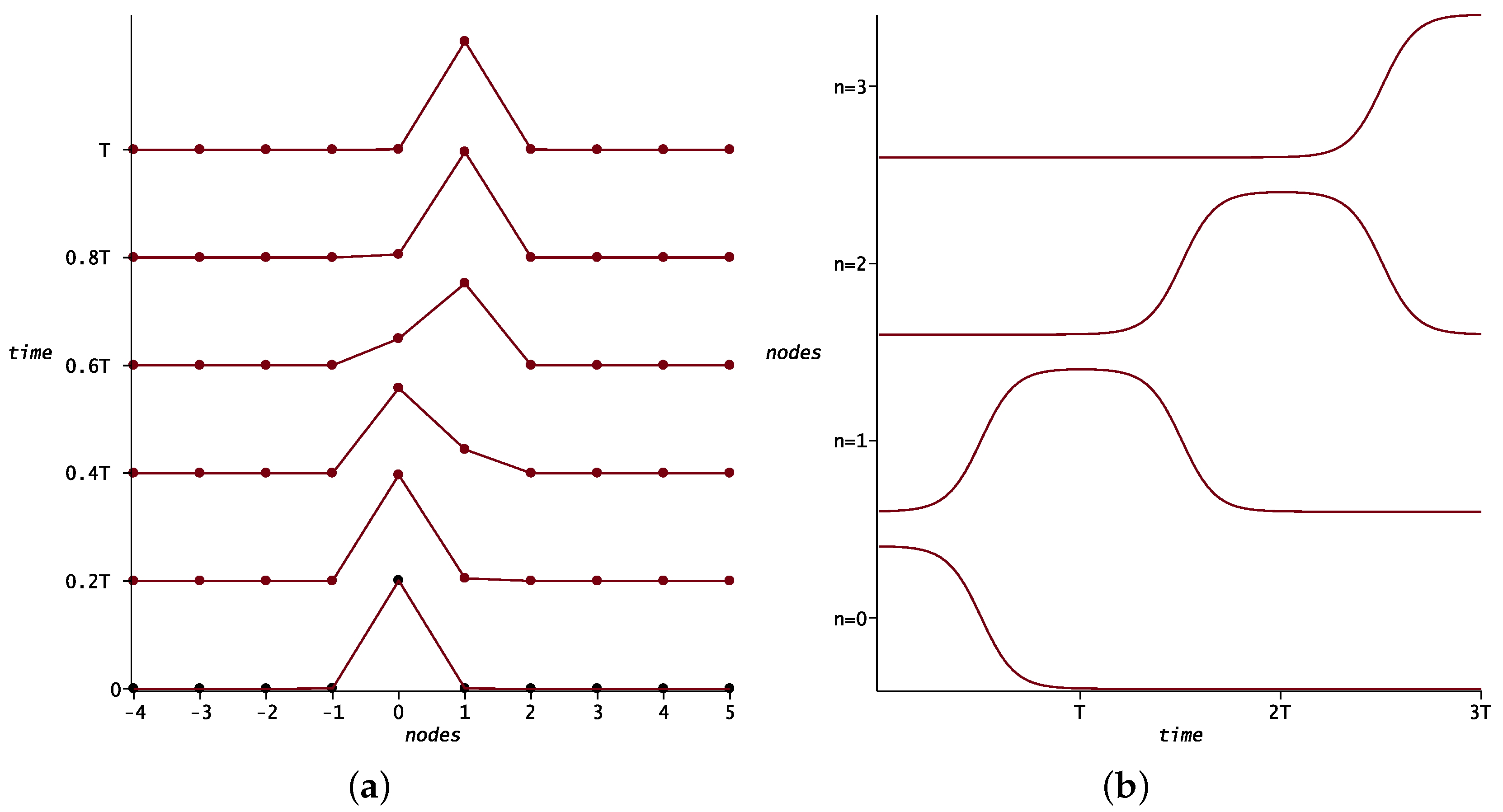
The value of exact solutions decreases if they are unstable to small deviations. Naturally, these deviations are introduced, for example, by the finite-difference approximation of the time derivative used in the numerical construction of solutions. The invariance of the shape of the traveling-wave solution for a sufficient period of time indicates both the convergence of the applied difference scheme and the correctness of the analytical solution of the problem. Figure 6 shows the evolution of the solution of Equation (1) with the initial condition, the graph of which is shown in Figure 1a (impulse with a sharp peak); Figure 7 corresponds to the initial condition from Figure 1b. The symbol T denotes the period of oscillation $T=\frac{d}{\omega }$. To calculate the solution, the continuous 7–8 orders Runge–Kutta method, built into the Maple software package, was used.

As we see in Figure 6b and Figure 7b, dependences $u_n(t)$ for all nodes are identical and coincide in form with the solution (1.10), the graphs of which are shown for some combinations of parameters in Figure 1. It can be seen from Figure 7a that over the time T the graph is completely restored to its shape, as it should be for a traveling wave solution.

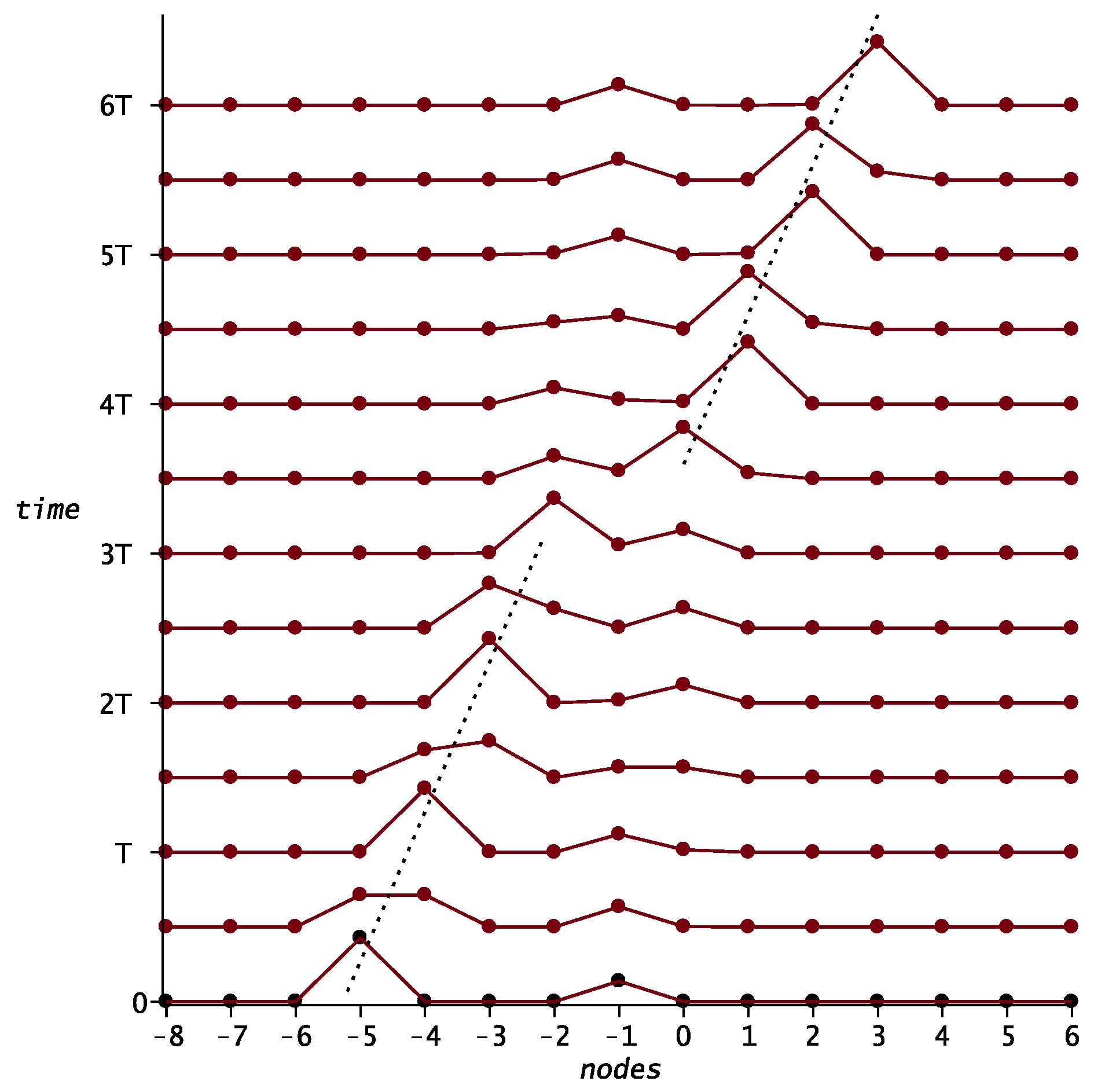
Figure 8 shows the interaction of two solitary waves of different amplitudes. The collision of waves occurs according to the elastic scenario, with a complete restoring of the shape and amplitude of each wave and a certain phase shift—the catching-up wave shifts forward in the direction of travel, and the catch-up wave shifts backward. The process is completely identical to that observed for solitons of the KdV equation.

Numerical modeling of the periodic solution (1.12), (1.19) for two values $D=0.01$ and $D=0.49$, for which Figure 3 was constructed, showed that the solution form does not visually change over more than 100 oscillation periods.

7. Discussion

The geometric series method is designed to search for exact DDE solutions, and the solutions found are expressed in terms of the ratio of two polynomials in powers of the exponential function. As repeatedly noted by leading experts [25], there is no universal approach to finding the exact solutions of nonlinear equations. The closest to the geometric series method should be considered the method of exponential functions (exp-function method) [25,26,27,28] and the method of hyperbolic tangent (tanh-method) [16,17,29]. The exp-function method uses an ansatz in the form of a ratio of two polynomials in powers of an exponential function with arbitrary coefficients. After substituting the ansatz in the equation, it is required that in the numerator of the obtained expression the factors at each degree of the exponential function vanish. This requirement leads to the need to solve a system of nonlinear algebraic equations for the coefficients. Unfortunately, the nonlinear system of the exp-function method is successfully solved by modern computer mathematics systems only in the simplest cases [5]. In particular, in the case of the discrete Sawada–Kottera equation under consideration, a calculation in Maple 2016.2 for one hour on a 6-core AMD Ryzen 5 4.2 GHz workstation with 16 Gb of RAM, did not lead to any results. Unlike the exp-function method, the geometric series method is based on the sequential solution of a system of linear equations and the exact solution (10) of the discrete Sawada–Kotera equation is successfully detected within a few seconds.

The tanh-method uses an ansatz in the form of a polynomial in powers of the hyperbolic tangent, the highest degree of which is consistent with the pole order of the desired solution. If tanh(z) is expressed in terms of exp(z), then the tanh-method ansatz is represented by the ratio of two polynomials in powers of exp(z), as in the geometric series method. However, it is easy to verify that solution (10) cannot be represented by any finite polynomial in powers of tanh(z) and, therefore, cannot be obtained in principle by the tanh-method.

Sometimes an explicit form of exact DDE solutions can be obtained using Darboux transforms of the corresponding Lax pairs [30], however, this is a much more time-consuming procedure compared to the proposed direct method.

A review of available publications on the problem could not reveal solutions of the discrete Sawada–Kotera equation, the structure of which coincides with Equation (10). It can be argued that Equation (10) is a new solution. As far as we know, the exact periodic solution (12), (19) and the initial problem solution (27) were also obtained for the first time.

8. Conclusions

In this article, a number of problems are solved for an integrable discrete Sawada–Kotera equation. For the first time using the geometric series method, its exact solitary-wave solution in explicit form was constructed and numerical modeling was carried out, revealing its soliton properties. Exact periodic solutions are obtained in terms of the Jacobi elliptic function. When solving the problem with special initial conditions, new combinatorial dependencies were identified that connect the desired solution with the generating function for Catalan numbers. So far, questions remain about the possibility of constructing rational solutions, as well as exact solutions of DDE systems by the geometric series method. In the future, it may be able to study the problems of classifying exact solutions of integrable DDEs and constructing quasi-exact and approximate solutions of some non-integrable equations.

References

Mikhailov, A.V.; Wang, J.P.; Xenitidis, P. Recursion operators, conservation laws, and integrability conditions for difference equations. Theor. Math. Phys.2011, 167, 421–443. [Google Scholar] [CrossRef]
Tsuchida, T. Integrable discretizations of derivative nonlinear Schrodinger equations. J. Phys. A Math. Gen.2002, 35, 7827. [Google Scholar] [CrossRef][Green Version]
Garifullin, R.N.; Yamilov, R.I.; Levi, D. Classification of five-point differential–difference equations II. J. Phys. A Math. Theor.2018, 51, 065204. [Google Scholar] [CrossRef]
Yamilov, R.I. On classification of discrete evolution equations. Uspekhi Mat. Nauk1983, 38, 155–156. [Google Scholar]
Yamilov, R.I. Symmetries as integrability criteria for differential difference equations. J. Phys. A2006, 39, R541. [Google Scholar] [CrossRef]
Suris, Y.B. The Problem of Integrable Discretization: Hamiltonian Approach; Birkhauser: Basel, Switzerland, 2003. [Google Scholar]
Adler, V.E. On a discrete analog of the Tzitzeica equation. arXiv2011, arXiv:1103.5139v1. [Google Scholar]
Sawada, K.; Kotera, T. A method for finding n-soliton solutions of the KdV equation and KdV-like equations. Progr. Theor. Phys.1974, 51, 1355–1367. [Google Scholar] [CrossRef]
Tsujimoto, S.; Hirota, R. Pfaffian representation of solutions to the discrete BKP hierarchy in bilinear form. J. Phys. Soc. Jpn.1996, 65, 2797–2806. [Google Scholar] [CrossRef]
Gubbiotti, G. Algebraic entropy of a class of five-Point differential-difference equations. Symmetry2019, 11, 432. [Google Scholar] [CrossRef]
Baldwin, D.; Goktas, U.; Hereman, W. Symbolic computation of hyperbolic tangent solutions for nonlinear differential–difference equations. Comp. Phys. Comm.2004, 162, 203–217. [Google Scholar] [CrossRef]
Baldwin, D.; Goktas, U.; Hereman, W.; Hong, L.; Martino, R.S.; Millere, J.C. Symbolic computation of exact solutions expressible in hyperbolic and elliptic functions for nonlinear PDEs. J. Symb. Comp.2004, 37, 669–705. [Google Scholar] [CrossRef]
Bochkarev, A.V.; Zemlyanukhin, A.I. The geometric series method for constructing exact solutions to nonlinear evolution equations. Comp. Math. Math. Phys.2017, 57, 1111–1123. [Google Scholar] [CrossRef]
Zemlyanukhin, A.I.; Bochkarev, A.V. Continued fractions, the perturbation method and exact solutions to nonlinear evolution equations. Izvestiya VUZ. Appl. Nonlin. Dyn.2016, 24, 71–85. [Google Scholar] [CrossRef]
Zhang, S. Exp-function method for constructing explicit and exact solutions of a lattice equation. Appl. Math. Comput.2008, 199, 242–249. [Google Scholar] [CrossRef]
Zhang, S.; Li, J.; Zhou, Y. Exact solutions of non-linear lattice equations by an improved exp-function method. Entropy2015, 17, 3182–3193. [Google Scholar] [CrossRef]
Parkes, E.J.; Duffy, B.R. An automated tanh-function method for finding solitary wave solutions to non-linear evolution equations. Comput. Phys. Commun.1996, 98, 288–300. [Google Scholar] [CrossRef]
Xu, X.-X. Solving an integrable coupling system of Merola–Ragnisco–Tu lattice equation by Darboux transformation of Lax pair. Commun. Nonlin. Sci. Numer. Simul.2015, 23, 192–201. [Google Scholar] [CrossRef]
Figure 1.
(a) pulse with a sharp peak at , , . (b) pulse with a flat peak at , , .
Figure 2.
Dependencies (solid line) and (dashed line).
Figure 3.
Profiles of a traveling periodic wave (12): (a) , (b) .
Figure 4.
Dependence , calculated according to (27) for .
Figure 5.
Variant of a periodic stationary solution.
Figure 6.
The solution of Equation (1) with the initial condition from Figure 1a. (a) the wave profile at different points in time; (b) the dependences for some nodes.
Figure 7.
The solution of Equation (1) with the initial condition from Figure 1b. (a) the wave profile at different points in time; (b) the dependences for some nodes.
Figure 8.
Collision of two solitary waves (10) with parameters , , (catching wave of greater amplitude) and , , (wave of smaller amplitude). The dashed line shows the line of the constant phase of the larger wave; the time scale is indicated in the periods T of recovery of the larger wave.
Zemlyanukhin, A.; Bochkarev, A.