Flexible Birnbaum–Saunders Distribution

Abstract

In this paper, we propose a bimodal extension of the Birnbaum–Saunders model by including an extra parameter. This new model is termed flexible Birnbaum–Saunders (FBS) and includes the ordinary Birnbaum–Saunders (BS) and the skew Birnbaum–Saunders (SBS) model as special cases. Its properties are studied. Parameter estimation is considered via an iterative maximum likelihood approach. Two real applications, of interest in environmental sciences, are included, which reveal that our proposal can perform better than other competing models.

1. Introduction

The BS distribution was originally introduced in [1] to model the fatigue in the lifetime of certain materials. During the last decades, mainly due to its good properties, the use of this model spread out to other fields, such as economics and environmental sciences. In these applied scenarios, quite often, departures of the BS model are found, and therefore it is necessary to introduce some improvements. In this paper, we focus on those situations in which extra asymmetry or bimodality are present in our data, and a generalization of the BS model should be considered to deal with these issues. To reach this end, a flexible BS model is introduced. Our proposal is based on the flexible skew-normal distribution introduced in [2], and includes, as particular cases, the BS and skew BS distribution. Next, we briefly describe the key aspects that properly combined result in the flexible BS model. These are asymmetry, bimodality and main features of the basic BS model.

1.1. Asymmetry

Earlier results on asymmetric models started with the pioneering works by [1,3,4]. This topic regained interest with the study in [5], which from a Bayesian point of view developed a new asymmetric model which was later studied in depth by Azzalini [6], from a classical point of view. Azzalini model was termed the skew-normal distribution. Following Azzalini’s method, a general family of asymmetric models termed skew-symmetric models appeared in the literature. The following lemma, originally presented in [6], can be considered as the starting point for the development of these asymmetric models.

Lemma 1.

Let $f_0$ be a probability density function (pdf) which is symmetric around zero, and G a cumulative distribution function (cdf) such that $G^{\prime }$ exists and is a symmetric pdf around zero. Then

$$\begin{array}{c}\hfill f_Z(z;\lambda )=2f_0\left(z\right)G\left(\lambda z\right),z\in \mathbb{R},\end{array}$$

(1)

is a pdf for $\lambda \in \mathbb{R}$.

Equation (1) provides the skew version of $f_0(·)$ with skewing function $G(·)$ and $\lambda$ the skewness parameter. If $f_0(·)=\varphi (·)$ and $G(·)=\Phi (·)$, the pdf and cdf, respectively, of the $N(0,1)$ distribution, then the skew-normal is obtained, whose pdf is

$$f_Z\left(z\right)=2\varphi \left(z\right)\Phi \left(\lambda z\right),z\in \mathbb{R},\lambda \in \mathbb{R}.$$

(2)

Other examples of skew models are: skew-t, skew-Cauchy, skew-elliptical, and generalized skew-elliptical. We highlight that all of them are unimodal distributions.

1.2. Bimodality

Another fundamental result in our proposal will be the following lemma, which was given in Gómez et al. [2]. These authors extended (1), by introducing a parameter $\delta$ in $f_0$, in such a way that for certain values of $\delta$ the resulting distribution is bimodal.

Lemma 2.

Let f be a symmetric pdf around zero, F the corresponding cdf and G an absolutely continuous cdf such that $G^{\prime }$ exists and is symmetric around zero. Then

$$\begin{array}{c}\hfill g(z;\delta ,\lambda )=c_{\delta }f(\left|z\right|+\delta )G\left(\lambda z\right),z\in \mathbb{R},\lambda ,\delta \in \mathbb{R}\end{array}$$

(3)

is a pdf and $c_{\delta }^{-1}=1-F\left(\delta \right).$

Taking $f(·)=\varphi (·)$ and $G(·)=\Phi (·)$, in (3), the flexible skew-normal (FSN) model was obtained and studied in detail in [2]. There, it was proved that the FSN model can be bimodal for certain values of $\delta .$ Notice that the FSN model is obtained by adding an extra parameter, $\delta$, to the skew-normal distribution proposed in [6]. That is a random variable (rv) Z follows a FSN distribution, $Z\sim FSN(\delta ,\lambda ),$ if its pdf is given by

$$\begin{array}{c}\hfill f(z;\delta ,\lambda )=c_{\delta }\varphi (\left|z\right|+\delta )\Phi \left(\lambda z\right),z\in \mathbb{R},\lambda ,\delta \in \mathbb{R}\end{array}$$

(4)

where $\varphi$ and $\Phi$ are the pdf and cdf of the $N(0,1)$ distribution, respectively, and $c_{\delta }^{-1}=1-\Phi \left(\delta \right).$

Other recent proposals in the contemporary literature dealing with bimodality are the extended two-pieces skew-normal model (ETN), introduced in [7] and the uni-bi-modal asymmetric power normal model given in [8] whose properties are based on results given in [9,10]. Applications of interest in Economics are given in [11]. All these references show the interest in the latest years for modelling bimodality.

1.3. BS Model

The BS or fatigue life distributions was proposed for modelling survival time data and material lifetime subject to stress in [12,13]. This model is asymmetric and only fits positive data. The pdf of a BS distribution is given by

$$\begin{array}{c}\hfill f_T\left(t\right)=\varphi \left(a_t\right)\frac{t^{-3/2}(t+\beta )}{2\alpha \sqrt{\beta }},t>0,\end{array}$$

(5)

where

$$a_t=a_t(\alpha ,\beta )=\frac{1}{\alpha }\left(\sqrt{\frac{t}{\beta }}-\sqrt{\frac{\beta }{t}}\right),$$

(6)

$\alpha >0$ is a shape parameter, $\beta >0$ is a scale parameter and the median of this distribution. (5) is denoted as $T\sim BS(\alpha ,\beta ).$ It is well known that $\alpha$ is the parameter that controls asymmetry. Specifically, (5) becomes more asymmetric as $\alpha$ increases and symmetric around $\beta$ as $\alpha$ gets close to zero. It can be seen in [13] that (5) can be obtained as the distribution of the random variable

$$\begin{array}{c}\hfill T=\beta {\left[\frac{\alpha }{2}Z+\sqrt{{\left(\frac{\alpha }{2}Z\right)}^2+1}\right]}^2,\end{array}$$

(7)

where $Z\sim N(0,1).$

The BS model has been applied to a variety of practical situations. However, quite often, although the data suggest a BS distribution, some deficiencies are observed in the fitted BS model. This problem has motivated an increasing interest in its generalizations. We highlight that, recently, this model was extended by [14] to the family of elliptical distributions, this is known in the literature as the generalized Birnbaum–Saunders (GBS) distribution. Later, [15] proposed an extension based on the elliptical asymmetric distributions, known as the doubly generalized Birnbaum–Saunders model. On the other hand, [16] presents the asymmetric BS distribution with five parameters called the extended Birnbaum–Saunders (EBS) distribution. Other types of extensions are the asymmetric epsilon-Birnbaum–Saunders model given in [17], models in [18] based on the slash-elliptical family of distributions, and the generalized modified slash Birnbaum–Saunders (GMSBS) proposed in [19], which is based on [20].

In these extensions, we find that the asymmetric BS models previously cited, such as [15,21], are designed to fit data with greater or smaller asymmetry (or kurtosis) than that of the ordinary BS model, but they are not appropriate for fitting bimodal data. On the other hand, we highlight that the extension given in [21], which can become bimodal for certain combination of parameters is unable to capture bimodality unless it is accentuated enough.

Therefore there exists a real need for an asymmetric model, based on the BS distribution, and able to fit data presenting bimodal features, which is not uncommon in the literature. So the present paper presents a flexible BS distribution able to model skewness and to fit data with and without bimodality.

The paper is organized as follows. Section 2 is devoted to the development of an asymmetric uni-bimodal BS model. Its properties are studied in depth. Specifically, a closed expression for the cumulative distribution function (cdf) is given in terms of the cdf of a bivariate normal distribution. Some of the models proposed in [15,22] are obtained as particular cases. The shape and bimodality of the distribution are studied. It is shown that this model is closed under a change of scale and reciprocity. Survival and hazard functions are also obtained. Section 3 deals with moments derivation and iterative maximum likelihood estimation methods for the new model. Section 4 is devoted to real data applications of interest in environmental sciences. The first one deals with a bimodal situation in which our proposal performs better than other BS models and a mixture of normal distributions. The second one is taken from [16], where the extended BS model was proposed as the best for this dataset. It is shown that the FBS outperforms the extended BS model.

2. Results in Flexible Birnbaum-Saunders

Based on the flexible skew-normal model proposed in [2], we extend the Birnbaum–Saunders. The main idea is to apply (7) with $Z\sim FSN(\delta ,\lambda )$ introduced in (4). This new model is called the flexible Birnbaum–Saunders (FBS) distribution whose pdf is given by

$$f(t;\alpha ,\beta ,\delta ,\lambda )=\frac{t^{-3/2}(t+\beta )}{2\alpha {\beta }^{1/2}(1-\Phi \left(\delta \right))}\varphi \left(\right|a_t|+\delta )\Phi \left(\lambda a_t\right),$$

(8)

with $a_t$ defined in (6), $t>0$, $\alpha >0$, $\beta >0$, $\delta \in \mathbb{R}$, $\lambda \in \mathbb{R}$, $\varphi (·)$ and $\Phi (·)$ the pdf and cdf of a $N(0,1)$, respectively. We use the notation $T\sim FBS(\alpha ,\beta ,\delta ,\lambda ).$ The inclusion of parameters $\delta$ and $\lambda$ makes our approach more flexible than the extensions previously discussed. $\lambda$ is a parameter that controls asymmetry (skewness) and $\delta$ is a shape parameter related to bimodality of our proposal.

If $\lambda =0$ then we obtain, as a particular case, the model introduced by [22].

Figure 1 and Figure 2 depict the behaviour of (8) for some values of parameters, illustrating that it can be bimodal for some combinations of them.

2.1. Interpretation of Parameters.

In both figures the values of parameters $\alpha$ and $\beta$ are fixed. We study the effects of

(i)

$\lambda$ positive versus $\lambda$ negative.

(ii)

Increasing $\delta >0$ in Figure 1. Decreasing $\delta <0$ in Figure 2.

Figure 1 suggests that, for $\alpha$ and $\beta$ fixed, if a positive value of $\delta$ is considered then we have a unimodal distribution and the peak of the distribution increases when $\delta$ increases: $\delta =0.75$ (red solid line), $\delta =1.5$ (green dashed line), …, $\delta =3$ (blue dashed dotted line). This happens for positive and negative values of $\lambda$.

On the other hand, in Figure 2, we have different situations. This plot suggests that, for $\alpha$ and $\beta$ fixed, if a negative value of $\delta$ is considered then a bimodal distribution can be obtained. For positive $\lambda$, if $\delta$ decreases: $\delta =-0.75$ (red solid line), $\delta =-1.5$ (green dashed line), …, $\delta =-3$ (blue dashed dotted line), then the peaks decrease and bimodality becomes more accentuated. For negative $\lambda$, if $\delta$ decreases, then main peak increases and bimodality becomes less accentuated.

Also, note in Figure 1 and Figure 2, that in the FBS model the pdf for negative $\lambda$ is no longer the specular image of plot for positive $\lambda$.

2.2. Properties

Next, important properties of the FBS model are presented. First an explicit expression for the cdf is given in terms of the cdf of a bivariante normal distribution.

Proposition 1.

Let $T\sim FBS(\alpha ,\beta ,\delta ,\lambda )$. Then the cdf of T is

$$F_T\left(t\right)=\left\{\begin{array}{cc}{c}_{\delta }{\Phi }_{B{N}_{\lambda }}\left(\frac{\lambda \delta }{\sqrt{1+{\lambda }^2}},a_t-\delta \right),\hfill & \mathrm{if}0<t<\beta \hfill \\ c_{\delta }\left[{\Phi }_{B{N}_{\lambda }}\left(\frac{\lambda \delta }{\sqrt{1+{\lambda }^2}},-\delta \right)+{\Phi }_{B{N}_{\lambda }}\left(-\frac{\lambda \delta }{\sqrt{1+{\lambda }^2}},a_t+\delta \right)-{\Phi }_{B{N}_{\lambda }}\left(-\frac{\lambda \delta }{\sqrt{1+{\lambda }^2}},\delta \right)\right],\hfill & \mathrm{if}t\ge \beta ,\hfill \end{array}\right.$$

(9)

where ${\Phi }_{B{N}_{\lambda }}(x,y)$ is the cdf of a bivariate normal distribution, with mean vector ${\mathit{\mu }}^{\prime }=(0,0)$ and covariance matrix

$${\Omega }_{\lambda }=\left(\begin{array}{ccc}1& & {\rho }_{\lambda }\\ {\rho }_{\lambda }& & 1\end{array}\right)\mathit{where}{\rho }_{\lambda }=-\frac{\lambda }{\sqrt{1+{\lambda }^2}}.$$

(10)

Proof. 

It can be seen in Appendix A. □

Next some particular cases of interest for $\lambda$ and $\delta$ parameters are discussed. Results about the shape of $f_T(·)$ are included.

2.2.1. Effect of $\lambda$.

Corollary 1.

Let $T\sim FBS(\alpha ,\beta ,\delta ,\lambda )$. If $\lambda =0$ then the cdf of T is

$$F_T\left(t\right)=\left\{\begin{array}{cc}\frac{c_{\delta }}{2}\Phi (a_t-\delta ),\hfill & if0<t<\beta \hfill \\ \frac{c_{\delta }}{2}\left\{\Phi (a_t+\delta )+1-2\Phi \left(\delta \right)\right\},\hfill & ift\ge \beta .\hfill \end{array}\right.$$

(11)

Proof. 

If $\lambda =0$ then ${\rho }_{\lambda }$, defined in (10), is equal to zero, and since in the bivariate normal distribution uncorrelation implies independence, we have that

$${\Phi }_{B{N}_{\lambda =0}}(x,y)=\Phi \left(x\right)\Phi \left(y\right),\forall (x,y).$$

Taking into account that $\Phi \left(0\right)=1/2$ and $\Phi (-\delta )=1-\Phi \left(\delta \right)$, we have that (9) reduces to (11). □

Result in Corollary 1 corresponds to the model studied in [22].

2.2.2. Effect of $\delta$.

Corollary 2.

Let $T\sim FBS(\alpha ,\beta ,\delta ,\lambda )$. If $\delta =0$ then $F_T$ reduces to $F_T\left(t\right)=2{\Phi }_{B{N}_{\lambda }}(0,a_t),$ for $t>0.$

Corollary 2 is a particular case of models studied in [15].

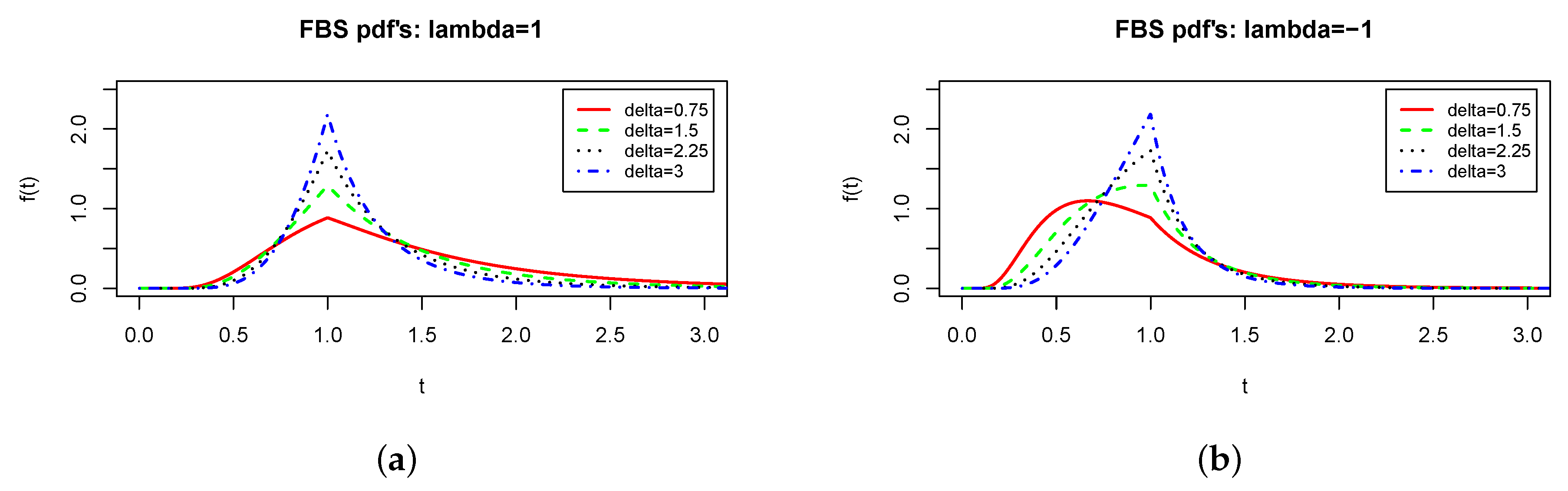
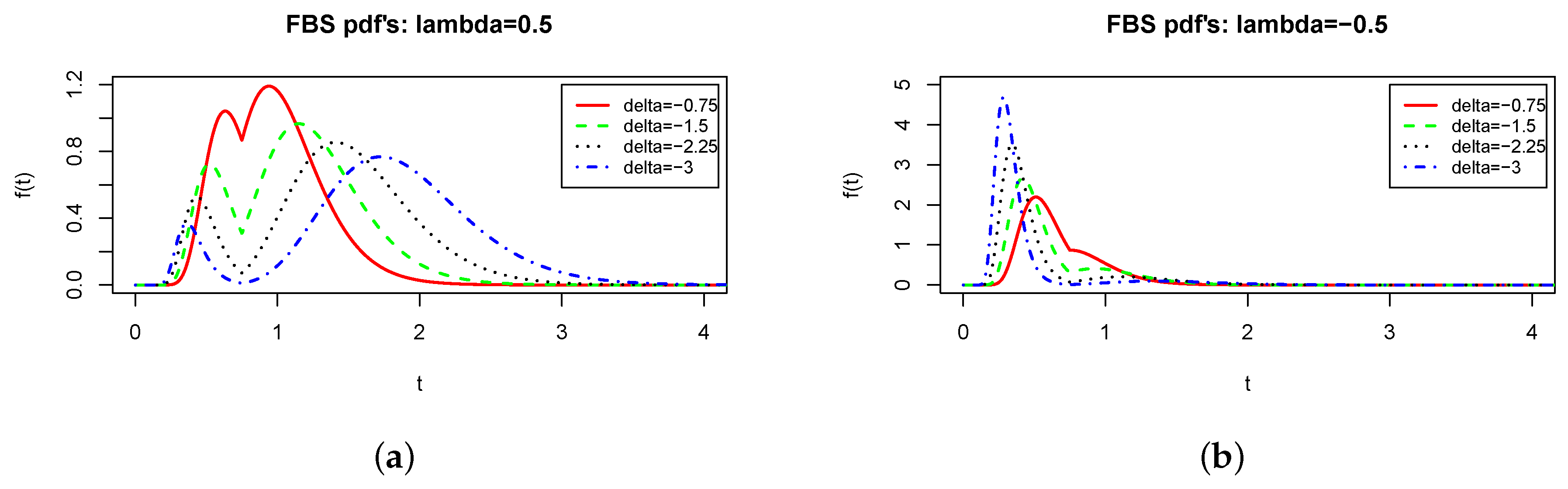
2.2.3. Shape of $f_T(·)$.

Proposition 2.

Let $T\sim FBS(\alpha ,\beta ,\delta ,\lambda ).$ Then the pdf given in (8) is nondifferentiable at $t=\beta .$

Proof. 

It follows from (8), by noting that if $t=\beta$ then $a_t=0$ and the absolute value function is not differentiable at zero. □

Proposition 3.

Let $T\sim FBS(\alpha ,\beta ,\delta ,\lambda ).$ The pdf given in (8) can be bimodal. The modes are the solution of the following non-linear equations.

1.

$0<t_1^{*}<\beta$ solution of

$$a_{t_1}=\delta +\lambda \frac{\varphi \left(\lambda a_{t_1}\right)}{\Phi \left(\lambda a_{t_1}\right)}+\frac{a_{t_1}^{″}}{{\left\{a_{t_1}^{\prime }\right\}}^2}.$$

(12)

2.

$t_2^{*}>\beta$ solution of

$$a_{t_2}=-\delta +\lambda \frac{\varphi \left(\lambda a_{t_2}\right)}{\Phi \left(\lambda a_{t_2}\right)}+\frac{a_{t_2}^{″}}{{\left\{a_{t_2}^{\prime }\right\}}^2},$$

(13)

With $a_t$ given in (6), $a_t^{\prime }$ and $a_t^{″}$ the first and second derivatives of $a_t$ with respect to t, respectively.

Proof. 

It is given in Appendix A. □

Comments on the use of (12) and (13) are included in Appendix A, Remark A1.

Remark 1.

Equations obtained in (12) and (13) are similar to those we have in the skew normal and BS model.

1.

Let $Z\sim SN\left(\lambda \right)$, $\lambda \in \mathbb{R}$. Then Z is unimodal and the mode, $z^{*}$, is given by the solution of the non-linear equation

$$z=\lambda \frac{\varphi \left(\lambda z\right)}{\Phi \left(\lambda z\right)}.$$

2.

Let $T\sim BS(\alpha ,\beta )$, $\alpha ,\beta >0.$ Then T is unimodal and the mode, $t^{*}$, is given by the solution of the non-linear equation

$$-a_t{\left\{a_t^{\prime }\right\}}^2+a_t^{{}^{″}}=0.$$

Next it is shown that the p-th quantile of T can be given in terms of the $pth$ quantile of the $FSN(\delta ,\lambda )$. Also it is proved that the FBS model is closed under change of scale and reciprocity.

Theorem 1.

Let $T\sim FBS(\alpha ,\beta ,\delta ,\lambda )$, with $\alpha ,\beta \in {\mathbb{R}}^{+}$ and $\delta ,\lambda \in \mathbb{R}$. Then

(i) 

Let $t_p$ be the pth quantile of T, $0<p<1$.

$$t_p=\beta {\left(\frac{\alpha }{2}{z}_p+\sqrt{{\left(\frac{\alpha }{2}{z}_p\right)}^2+1}\right)}^2$$

(14)

where $z_p$ denotes the pth quantile of $Z\sim FSN(\delta ,\lambda ).$

(ii) 

$kT\sim FBS(\alpha ,k\beta ,\delta ,\lambda )$ for $k>0$.

(iii) 

$T^{-1}\sim FBS(\alpha ,{\beta }^{-1},\delta ,-\lambda )$.

Proof. 

It can be seen in Appendix A. □

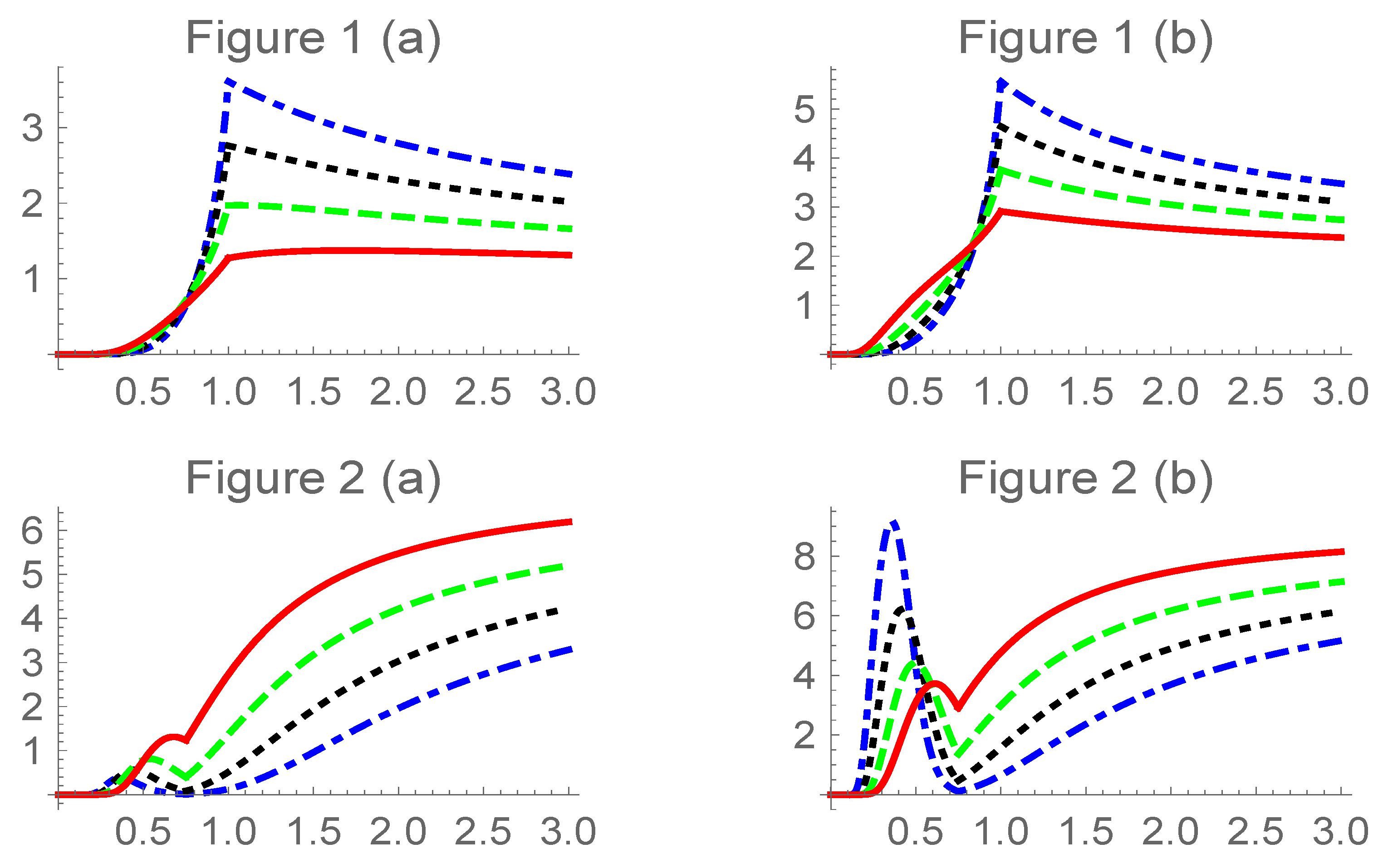
2.2.4. Lifetime Analysis

The BS model is commonly used to explain survival and material resistance data. The survival and risk (or hazard) functions are important indicators in such fields. For the FBS model these functions are given next.

Proposition 4.

Let $T\sim FBS(\alpha ,\beta ,\delta ,\lambda )$ with $\alpha ,\beta \in {\mathbb{R}}^{+}$ and $\delta ,\lambda \in \mathbb{R}$. Then

(i) 

The survival function is $S\left(t\right)=P[T>t]=1-F_T\left(t\right)$ with $F_T(·)$ given in (9).

(ii) 

The hazard function, $r\left(t\right)=f\left(t\right)/S\left(t\right)$, is

$$r\left(t\right)=\left\{\begin{array}{cc}\frac{c_{\delta }{a}_t^{\prime }\varphi \left(\right|a_t|+\delta )\Phi \left(\lambda a_t\right)}{1-c_{\delta }{\Phi }_{B{N}_{\lambda }}\left(\frac{\lambda \delta }{\sqrt{1+{\lambda }^2}},a_t-\delta \right)},\hfill & if0<t<\beta \hfill \\ \frac{c_{\delta }{a}_t^{\prime }\varphi \left(\right|a_t|+\delta )\Phi \left(\lambda a_t\right)}{1-c_{\delta }\left[{\Phi }_{B{N}_{\lambda }}\left(\frac{\lambda \delta }{\sqrt{1+{\lambda }^2}},-\delta \right)+{\Phi }_{B{N}_{\lambda }}\left(-\frac{\lambda \delta }{\sqrt{1+{\lambda }^2}},a_t+\delta \right)-{\Phi }_{B{N}_{\lambda }}\left(-\frac{\lambda \delta }{\sqrt{1+{\lambda }^2}},\delta \right)\right]},\hfill & ift\ge \beta \hfill \end{array}\right.$$

with ${\Phi }_{B{N}_{\lambda }}(·)$ the cdf of the bivariate normal given in Proposition 1.

In Figure 3, the hazard function for those pdf’s considered in Figure 1 and Figure 2 are plotted. These graphs show that, for the FBS distribution, the hazard function admits a variety of shapes, which is interesting from an applied point of view.

Remark 2.

More complicated hazard functions than the traditional ones are obtained when we are dealing with models with complex structure, as it happens with the FBS. For instance, in Figure 3, we have two situations:

1.

$r\left(t\right)$ corresponding to Figure 1a,b. These are, first, quickly increasing, later decreasing more slowly or even in a flat way. It can be applied in practical situations in which the risk of failure increases quickly until certain point in which its behaviour becomes flatter. As [23] points out, the flat area is very interesting in survival analysis and reliability contexts.

2.

$r\left(t\right)$ corresponding to Figure 2a,b are increasing-decreasing-increasing. This kind of hazard functions has been recently introduced and discussed in literature, due to its interest in reliability of systems, see for instance [23] or [24] (and references therein). In plot for Figure 2b, $r\left(t\right)$ is (quickly) increasing—or (quickly) decreasing. On the other hand, for Figure 2a the initial effect increasing—decreasing is less accentuated.

3. Moments and Maximum Likelihood Estimation

Moments of the FBS model can be obtained from the moments of the flexible skew-normal model given in [2]. The following results present important properties relating those distributions, and the expressions for the first moment and variance in the FBS model.

Theorem 2.

Let $T\sim FBS(\alpha ,\beta ,\delta ,\lambda )$ and $Z\sim FSN(\delta ,\lambda ).$ Then $\mathbb{E}\left(T^r\right)$, $r=0,1,\dots$, always exists. Moreover

$$\begin{array}{cc}\hfill \mathbb{E}\left(T^r\right)& =\frac{{\beta }^r}{4^r}\sum _{k=0}^{2r}\left(\genfrac{}{}{0pt}{}{2r}{k}\right)\mathbb{E}\left[{\left(\alpha Z\right)}^k{\left({\alpha }^2{Z}^2+4\right)}^{\frac{2r-k}{2}}\right],r=0,1,\dots .\hfill \end{array}$$

(15)

Proof. 

From (7), we can write

$$T=\frac{\beta }{4}{\left\{\alpha Z+{\left({\alpha }^2{Z}^2+4\right)}^{1/2}\right\}}^2.$$

Taking expectation of the rth-power of T

$$\begin{array}{c}\hfill \mathbb{E}\left(T^r\right)=\frac{{\beta }^r}{4^r}\mathbb{E}\left[{\left\{\alpha Z+{\left({\alpha }^2{Z}^2+4\right)}^{1/2}\right\}}^{2r}\right].\end{array}$$

(16)

From (16), note that for $r=0,1,\dots$, $\mathbb{E}\left(T^r\right)$ exists if and only if $\mathbb{E}\left(Z^{2r}\right)$ exists. On the other hand, it can be seen in [2] that $\mathbb{E}\left(Z^{2r}\right)$ always exists, and therefore $\mathbb{E}\left(T^r\right)$ too.

Finally note that (15) is the result of applying the binomial formula to (16). □

Next, explicit expressions for the expected value and variance of $T\sim FBS(\alpha ,\beta ,\delta ,\lambda )$ are given. In these expressions, ${\kappa }_j={\mathbb{E}}_{SFN}\left(\frac{Z^j}{2}\sqrt{{\alpha }^2{Z}^2+4}\right)$ with $Z\sim FSN(\delta ,\lambda )$.

Theorem 3.

Let $T\sim FBS(\alpha ,\beta ,\delta ,\lambda )$. Then

$$\begin{array}{c}\hfill \mathbb{E}\left(T\right)=\beta \left[1+\alpha {\kappa }_1+\frac{{\alpha }^2}{2}{c}_{\delta }\left\{(1+{\delta }^2)(1-\Phi \left(\delta \right))-\delta \varphi \left(\delta \right)\right\}\right],\end{array}$$

(17)

$$\begin{array}{cc}\hfill \mathbb{E}\left(T^2\right)& ={\beta }^2\left[\frac{7{\alpha }^4{c}_{\delta }}{16}\left((3+6{\delta }^2+{\delta }^4)(1-\Phi \left(\delta \right))-\delta (5+{\delta }^2)\varphi \left(\delta \right)\right)+{\alpha }^3{\kappa }_3+2\alpha {\kappa }_1+1\right]\hfill \\ \hfill & +2{\alpha }^2{\beta }^2{c}_{\delta }\left((1+{\delta }^2)(1-\Phi \left(\delta \right))-\delta \varphi \left(\delta \right)\right)\hfill \end{array}$$

and

$$\begin{array}{c}\mathrm{Var}\left(T\right)={\beta }^2\left[\frac{7{\alpha }^4{c}_{\delta }}{16}\left((3+6{\delta }^2+{\delta }^4)(1-\Phi \left(\delta \right))-\delta (5+{\delta }^2)\varphi \left(\delta \right)\right)+{\alpha }^3{\kappa }_3-{\alpha }^2{\kappa }_1+1\right]\\ -\frac{{\alpha }^2{\beta }^2{c}_{\delta }}{4}\left((1+{\delta }^2)(1-\Phi \left(\delta \right))-\delta \varphi \left(\delta \right)\right)\left({\alpha }^2{c}_{\delta }\left((1+{\delta }^2)(1-\Phi \left(\delta \right))-\delta \varphi \left(\delta \right)\right)+4(1-\alpha {\kappa }_1)\right)\end{array}$$

where ${\kappa }_j={\mathbb{E}}_{FSN}\left(\frac{Z^j}{2}\sqrt{{\alpha }^2{Z}^2+4}\right)$ and $Z\sim FSN(\delta ,\lambda )$.

Proof. 

These results follows from Theorem 2 and the expressions of ${\kappa }_j$, which have been computed by using the results for moments of $Z\sim FSN(\delta ,\lambda )$ obtained in [2].

As illustration, note that for the case $r=1$, (15) reduces to

$$\begin{array}{ccc}\hfill \mathbb{E}\left(T\right)& =& \frac{\beta }{4}\left[\mathbb{E}({\alpha }^2{Z}^2+4)+2\mathbb{E}\left(\left(\alpha Z\right)\sqrt{{\alpha }^2{Z}^2+4})\right)+\mathbb{E}\left({\alpha }^2{Z}^2\right)\right]\hfill \\ & =& \beta \left[1+\alpha {\kappa }_1+\frac{{\alpha }^2}{2}\mathbb{E}\left(Z^2\right)\right],\hfill \end{array}$$

it can be seen in [2] that $\mathbb{E}\left(Z^2\right)=c_{\delta }(1+{\delta }^2)\left(1-\Phi \left(\delta \right))-\delta \varphi (\delta )\right)$, and so (17) is obtained. □

3.1. Maximum Likelihood Estimators

Parameter estimation in the BS model has been the topic of interest in many papers. Among others, we mentioned [25,26,27]. To estimate the parameters in the usual BS model, the modified moment method (MME) and maximum likelihood (MLE) are commonly used. To start the maximum likelihood approach moment estimators are used which are given by

$$\begin{array}{c}\hfill {\widehat{\beta }}_M=\sqrt{sr},\end{array}\begin{array}{c}\hfill {\widehat{\alpha }}_M=\sqrt{2\left(\sqrt{\frac{s}{r}}-1\right)}.\end{array}$$

where $s=\frac{1}{n}{\sum }_{i=1}^n{t}_i$ and $r={\left(\frac{1}{n}{\sum }_{i=1}^n\frac{1}{t_i}\right)}^{-1}$ are the sample (arithmetic) and harmonic mean, respectively. Relevant aspects of this distribution such as its robustness with respect to parameter estimation and $O\left(n^{-1}\right)$ bias corrections for MLEs, can be seen in [25,26,27].

In the following, we discuss MLE estimation for the FBS model in depth. Thus, given n observations independent and identically distributed, $T_1,T_2,...,T_n$, with $T_i\sim FBS(\alpha ,\beta ,\delta ,\lambda ),$ the log-likelihood function for the parameter vector $\mathit{\theta }={(\alpha ,\beta ,\delta ,\lambda )}^{\prime }$ is given by

$$\begin{array}{cc}\hfill \ell \left(\mathit{\theta }\right)& =-n\left(log\left(\alpha \right)+\frac{1}{2}log\left(\beta \right)+log\left(1-\Phi \left(\delta \right)\right)\right)-\frac{3}{2}\sum _{i=1}^{n}log\left(t_i\right)+\sum _{i=1}^{n}log(t_i+\beta )\hfill \\ \hfill & -\frac{1}{2}\sum _{i=1}^n(a_{t_i}^2+2\delta |a_{t_i}|+{\delta }^2)+\sum _{i=1}^{n}log\left(\Phi \left(\lambda a_{t_i}\right)\right).\hfill \end{array}$$

(18)

To maximize $l\left(\mathit{\theta }\right)$ in $\mathit{\theta }$, consider the first derivatives of $l\left(\mathit{\theta }\right)$ with respect to $\alpha$, $\beta$, $\delta$ and $\lambda$, denoted as ${\dot{l}}_{\alpha }$, ${\dot{l}}_{\beta }$, ${\dot{l}}_{\delta }$ and ${\dot{l}}_{\lambda }$, respectively. From ${\dot{l}}_{\alpha }=0$, ${\dot{l}}_{\beta }=0$, ${\dot{l}}_{\delta }=0$ and ${\dot{l}}_{\lambda }=0$, the likelihood equations are given by

$$-n+\sum _{i=1}^n{a}_{t_i}^2-\delta \sum _{i=1}^n|a_{t_i}|-\lambda \sum _{i=1}^n{a}_{t_i}\frac{\varphi \left(\lambda a_{t_i}\right)}{\Phi \left(\lambda a_{t_i}\right)}=0$$

(19)

$$-\frac{n}{2\beta }+\sum _{i=1}^n\frac{1}{t_i+\beta }+\frac{1}{2\alpha {\beta }^{3/2}}\sum _{i=1}^n\left(sgn\left(a_{t_i}\right)\left(|a_{t_i}|+\delta \right)-\lambda \frac{\varphi \left(\lambda a_{t_i}\right)}{\Phi \left(\lambda a_{t_i}\right)}\right)\frac{t_i+\beta }{\sqrt{t_i}}=0$$

(20)

$$\delta -\frac{\varphi \left(\delta \right)}{1-\Phi \left(\delta \right)}=-\frac{1}{n}\sum _{i=1}^n|a_{t_i}|$$

(21)

$$\sum _{i=1}^n{a}_{t_i}\frac{\varphi \left(\lambda a_{t_i}\right)}{\Phi \left(\lambda a_{t_i}\right)}=0$$

(22)

in which $sgn(·)$ denotes the $sign$ function.

The solution to the previous system of equations must be obtained by iterative methods such as the Newton-Raphson or quasi-Newton procedures, which can be implemented using the statistical software R, [28].

As initial estimates of $\alpha$ and $\beta$ can be proposed the estimates of these parameters obtained in the basic BS model, denoted as ${\widehat{\alpha }}_0$ and ${\widehat{\beta }}_0$. These estimates can be plugged into (21) and (22) to obtain preliminar estimates of $\delta$ and $\lambda$, ${\widehat{\delta }}_0$ and ${\widehat{\lambda }}_0$, and so, start the recursion.

3.2. Expected and Observed Information Matrices

Recall that, the Fisher information matrix is given by

$$I\left(\mathit{\theta }\right)={\left(j_{i,j}\right)}_{i,j=\alpha ,\beta ,\delta ,\lambda },$$

which entries are equal to minus the second partial derivatives of the log-likelihood function given in (18) with respect to the parameters in the model. They are denoted as $j_{\alpha \alpha }=-\frac{{\partial }^2}{\partial {\alpha }^2}l\left(\mathit{\theta }\right)$, and so on. So we have

$$\begin{array}{c}\hfill j_{\alpha \alpha }=-\frac{n}{{\alpha }^2}+\frac{1}{{\alpha }^2}\sum _{i=1}^n\left(3a_{t_i}^2+2\delta \left|a_{t_i}\right|\right)+\frac{\lambda }{{\alpha }^2}\sum _{i=1}^n{a}_{t_i}{w}_i\left(2+\lambda a_{t_i}{B}_i\right),\end{array}$$

$$\begin{array}{c}\hfill j_{\beta \alpha }=-\frac{1}{{\alpha }^3{\beta }^2}\sum _{i=1}^n\left(\frac{{\beta }^2-t_i^2}{t_i}\right)+\frac{1}{2{\alpha }^2{\beta }^{3/2}}\sum _{i=1}^n\left(\delta sgn\left(a_{t_i}\right)+\lambda w_i(-1+\lambda a_{t_i}{B}_i)\right)\left(\frac{t_i+\beta }{\sqrt{t_i}}\right),\end{array}$$

$$\begin{array}{cc}\hfill j_{\beta \beta }& =-\frac{n}{2{\beta }^2}+\sum _{i=1}^n\frac{1}{t_i+\beta }+\frac{1}{{\alpha }^2{\beta }^3}\sum _{i=1}^n{t}_i+\frac{1}{4\alpha {\beta }^{5/2}}\sum _{i=1}^n(\delta sgn\left(a_{t_i}\right)-\lambda w_i)\left(\frac{3t_i+\beta }{\sqrt{t_i}}\right)\hfill \\ \hfill & +\frac{{\lambda }^2}{4{\alpha }^2{\beta }^{3/2}}\sum _{i=1}^n{w}_i{B}_i{\left(\frac{t_i+\beta }{\sqrt{t_i}}\right)}^2,\hfill \end{array}$$

$$\begin{array}{c}\hfill j_{\delta \alpha }=-\frac{1}{\alpha }\sum _{i=1}^n|a_{t_i}|,\end{array}\begin{array}{c}\hfill j_{\delta \beta }=-\frac{1}{2{\alpha }^2{\beta }^{3/2}}\sum _{i=1}^{n}sgn\left(a_{t_i}\right)\left(\frac{t_i+\beta }{\sqrt{t_i}}\right),\end{array}$$

$$\begin{array}{c}\hfill j_{\lambda \alpha }=\frac{1}{\alpha }\sum _{i=1}^n{a}_{t_i}{w}_i\left(1-\lambda a_{t_i}{B}_i\right),\end{array}\begin{array}{c}\hfill j_{\lambda \beta }=\frac{1}{2\alpha {\beta }^{3/2}}\sum _{i=1}^n{w}_i\left(1+\lambda a_{t_i}{B}_i\right)\left(\frac{t_i+\beta }{\sqrt{t_i}}\right),\end{array}$$

$$\begin{array}{cc}\hfill j_{\delta \delta }& =n\left(w_{\delta }(\delta -w_{\delta })+1\right),\hfill \end{array}\begin{array}{c}\hfill j_{\delta \alpha }=j_{\delta \beta }=j_{\lambda \delta }=0,\end{array}\begin{array}{c}\hfill j_{\lambda \lambda }=\sum _{i=1}^n{a}_{t_i}^2{w}_i{B}_i\end{array}$$

where $w=\frac{\varphi \left(\lambda a_t\right)}{\Phi \left(\lambda a_t\right)},$ $w_{\delta }=\varphi \left(\delta \right)/(1-\Phi \left(\delta \right))$ and $B=\lambda a_t+w.$

The Fisher (expected) information matrix would be obtained by computing the expected values of the above second derivatives. Taking in this matrix $\delta =\lambda =0,$ that is, $T\sim BS(\alpha ,\beta )$, and, using results in [21], we have

$$I\left(\mathit{\theta }\right)=\left(\begin{array}{cccc}\frac{2}{{\alpha }^2}& 0& -\frac{1}{\alpha }\sqrt{\frac{2}{\pi }}& 0\\ 0& {\alpha }^{-2}{\beta }^{-2}\left(1+\frac{\alpha q\left(\alpha \right)}{\sqrt{2\pi }}\right)& 0& \frac{1}{\sqrt{2\pi }}\frac{1}{\alpha {\beta }^{3/2}}{A}_1\left(t\right)\\ -\frac{1}{\alpha }\sqrt{\frac{2}{\pi }}& 0& 1-\frac{2}{\pi }& 0\\ 0& \frac{1}{\sqrt{2\pi }}\frac{1}{\alpha {\beta }^{3/2}}{A}_1\left(t\right)& 0& \frac{2}{\pi }\end{array}\right),$$

where $A_1\left(t\right)=\mathbb{E}\left(\frac{t_i+\beta }{\sqrt{t_i}}\right),$ $q\left(\alpha \right)=\alpha \sqrt{\frac{2}{\pi }}-\frac{\pi exp\left(\frac{2}{{\alpha }^2}\right)}{2}erfc\left(\frac{2}{\alpha }\right)$, with $erfc(·)$ the error function, i.e., $erfc\left(x\right)=\frac{2}{\sqrt{\pi }}{\int }_x^{\infty }exp(-t^2)dt$, see [29].

It can be shown that $\left|I\left(\mathit{\theta }\right)\right|\ne 0,$ so the Fisher information matrix is not singular at $\delta =\lambda =0.$

Hence, for large samples, the MLE, $\widehat{\mathit{\theta }}$, of $\mathit{\theta }$ is asymptotically normal, that is,

$$\sqrt{n}\left(\widehat{\mathit{\theta }}-\mathit{\theta }\right)\stackrel{\mathcal{L}}{⟶}{N}_4(\mathbf{0},I{\left(\mathit{\theta }\right)}^{-1}),$$

resulting that the asymptotic variance of the MLE, $\widehat{\mathit{\theta }}$, is the inverse of Fisher information matrix $I\left(\mathit{\theta }\right).$ Since the parameters are unknown, usually the observed information matrix is considered where the unknown parameters are estimated by ML.

Asymptotic confidence intervals for the parameters in the FBS model can be obtained from these results.

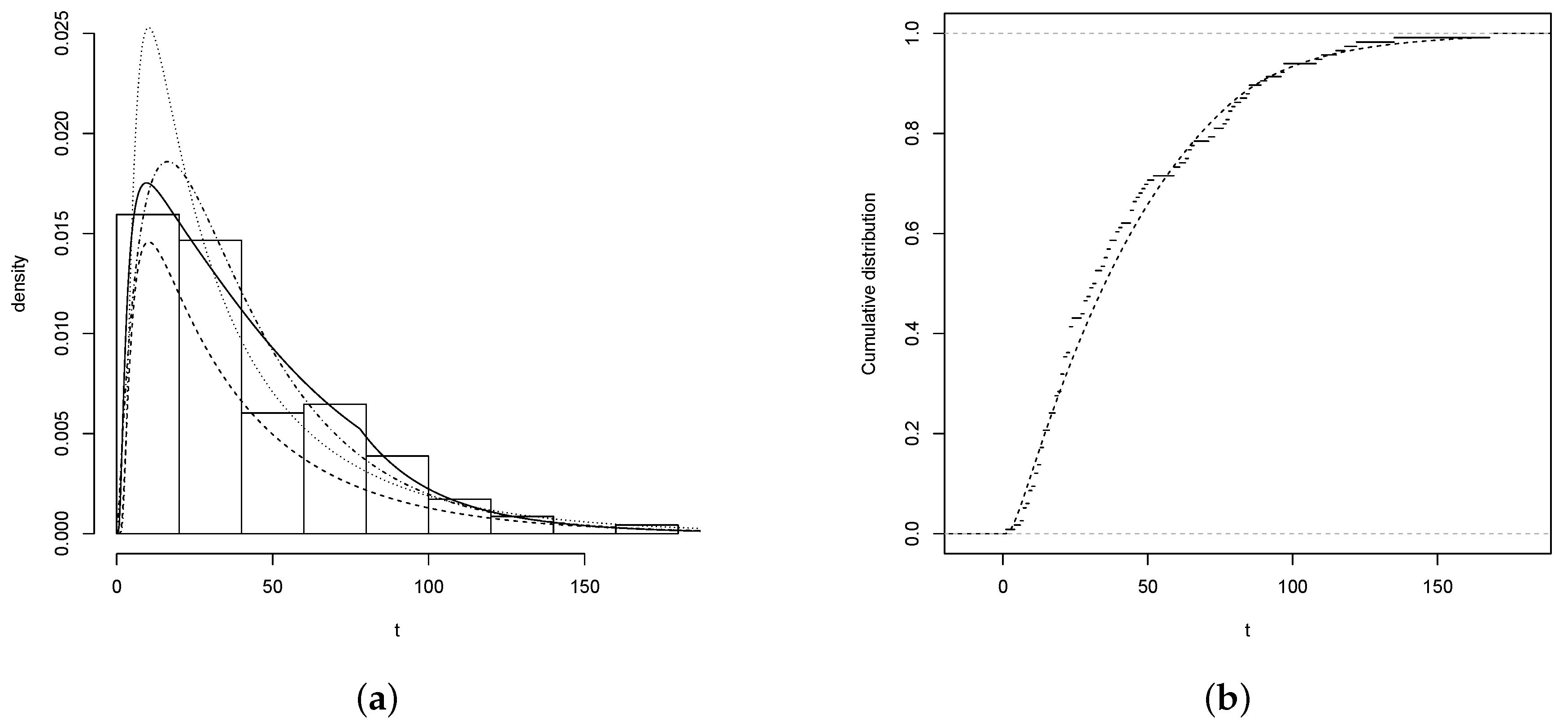
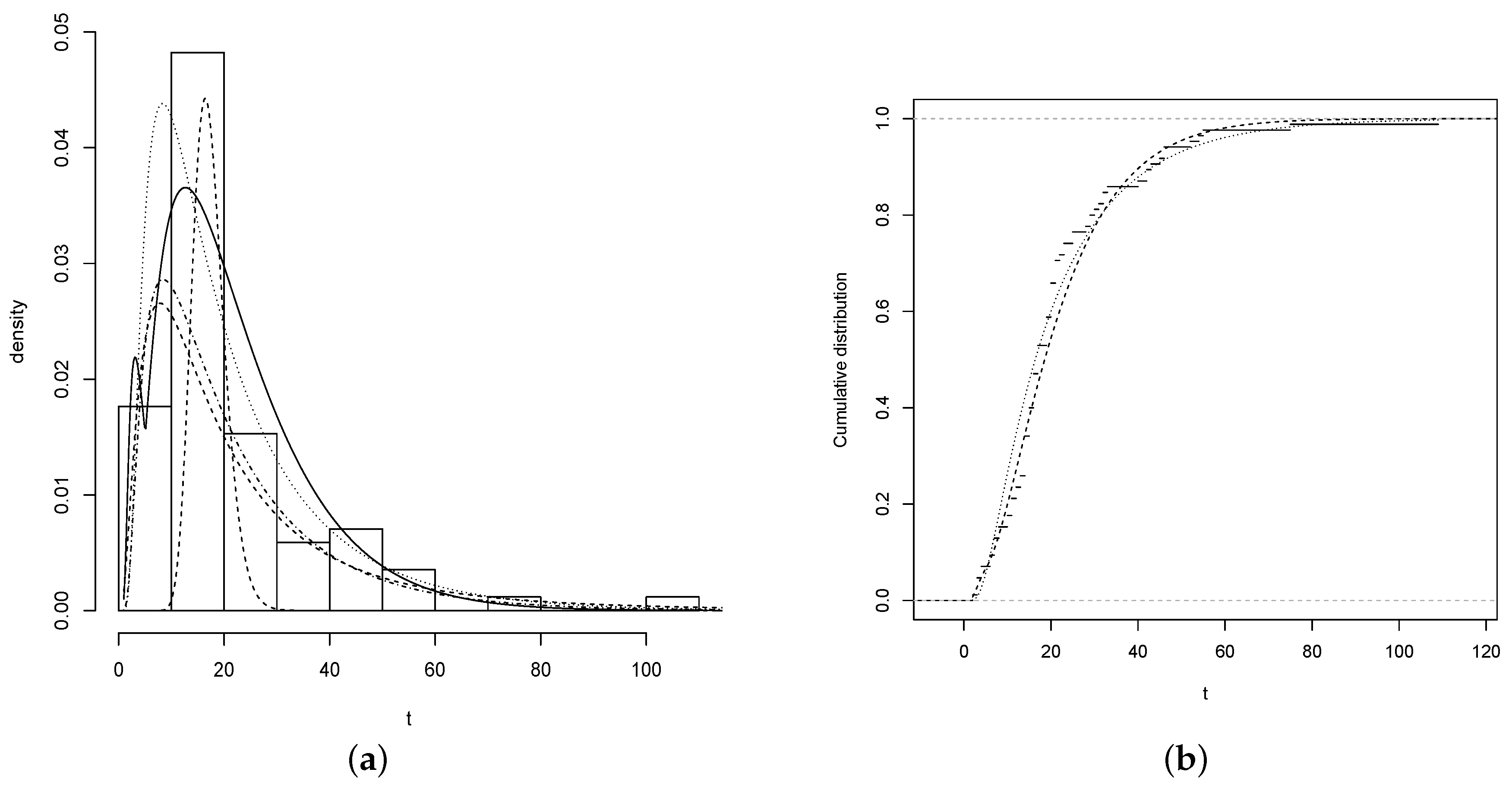
4. Numerical Illustrations

The numerical illustrations introduced next are aimed to show that the FBS model can be an alternative to modelling unimodal or bimodal data from different areas. First illustration is related to nickel content in soil samples analyzed at the Mining Department (Departamento de Minas) of Universidad de Atacama, Chile. We start by showing that both, BS and skew-BS (SBS) models are not able to capture bimodality present in this data set. Thus, the FBS model turned out to be a good option, to fit the data even better than a mixture of two normal distributions, which is another competing alternative to fit bimodal data. Second illustration is related to air pollution in New York city in USA, which was previously analyzed in [16,30]. In this case, it is shown that FBS model again provides a better fit than BS and SBS. As competing model the extended Birnbaum-Saunders (EBS) is also considered. Recall that the $EBS(\alpha ,\beta ,\sigma ,\nu ,\lambda )$ is a five-parameter model proposed in [16] where the parameter $\sigma$ affects the kurtosis; $\nu$ and $\lambda$ affect the skewness; and $\alpha$ and $\beta$ the shape and scale as in the usual BS model. We highlight that, for this dataset, the $FBS(\alpha ,\beta ,\delta ,\lambda )$ model provides a better fit than that given by the $EBS(\alpha ,\beta ,\sigma ,\nu ,\lambda )$ in [16] with the merit of using less parameters.

4.1. Nickel Concentration

For illustrative purposes, we apply the FBS model to a data set related to nickel content in soil samples. This data set encompasses 85 observations of the variable concentration of nickel with sample mean = 21.588, sample standard deviation = 16.573, sample asymmetry = 2.392 and sample kurtosis = 8.325, much higher than expected with the ordinary BS distribution.

4.1.1. FBS versus the BS and SBS distributions

To fit the nickel concentration variable, we use the BS, skew BS (SBS) and FBS models. Using function optim from the R-package, [28], the following point estimates (and their standard errors) are obtained for each of the three models under consideration

BS model: $\widehat{\alpha }=0.789\left(0.060\right)$ and $\widehat{\beta }=16.382\left(1.296\right).$

SBS model: $\widehat{\alpha }=1.073\left(0.201\right),$ $\widehat{\beta }=8.841\left(1.998\right)$ and $\widehat{\lambda }=1.252\left(0.590\right).$

FBS model: $\widehat{\alpha }=0.870\left(0.104\right),$ $\widehat{\beta }=5.072\left(0.763\right),$ $\widehat{\delta }=-1.520\left(0.282\right)$ and $\widehat{\lambda }=1.405\left(0.341\right).$

The bimodal hypothesis can be formally tested as follows

$$H_0:\delta =0\mathrm{versus}{H}_1:\delta \ne 0,$$

which is equivalent to compare models SBS versus FBS. Given the nonsigularity of the Fisher information matrix, and since these models are nested, we can consider the likelihood ratio statistics, namely

$${\Lambda }_1=L_{SBS}(\widehat{\alpha },\widehat{\beta },\widehat{\lambda })/L_{FBS}(\widehat{\alpha },\widehat{\beta },\widehat{\delta },\widehat{\lambda }).$$

It is obtained $-2log\left({\Lambda }_1\right)=5.618,$ which is greater than the $5\%$ chi-square critical value with one degree of freedom (df), which is equal to $3.84.$ Therefore, the null hypothesis of no-bimodality is rejected at the 5% critical level, leading to the conclusion that FBS model fits better than the unimodal SBS model to the nickel concentration data.

To compare the FBS model with the BS model, consider to test the null hypothesis of a BS distribution versus a FBS distribution, that is

$$H_0:(\delta ,\lambda )=(0,0)\mathrm{vs}{H}_1:(\delta ,\lambda )\ne (0,0)$$

using the likelihood ratio statistics based on the ratio ${\Lambda }_2=L_{BS}(\widehat{\alpha },\widehat{\beta })/L_{FBS}(\widehat{\alpha },\widehat{\beta },\widehat{\delta },\widehat{\lambda })$. After substituting the estimated values, we obtain $-2log\left({\Lambda }_2\right)=7.628,$ which is greater than the 5% chi-square critical value with 2 df, which is $5.99.$ Therefore the FBS is preferred to BS model for this data set.

4.1.2. FBS versus a Mixture of Normal Distributions

Another model widely applied in such situations of bimodality is the mixture of two normal distributions. The normal mixture model is given by:

$$f(x;{\mu }_1,{\sigma }_1,{\mu }_2,{\sigma }_2,p)=p{f}_1(x,{\mu }_1,{\sigma }_1)+(1-p)f_2(x;{\mu }_2,{\sigma }_2)$$

(23)

where $f_j$ is a normal distribution with parameters $({\mu }_j,{\sigma }_j)$, $j=1,2$ and $0<p<1.$ (23) is denoted by MN $({\mu }_1,{\sigma }_1,{\mu }_2,{\sigma }_2,p)$.

To compare FBS model with the MN model, we propose the Akaike information criterion (AIC), see [31], namely $AIC=-2\widehat{\ell }(·)+2k$, the modified AIC criterion (CAIC), typically called the consistent AIC, namely $CAIC=-2\widehat{\ell }(·)+(1+log\left(n\right))k$ and the Bayesian Information Criterion, BIC, $BIC=-2\widehat{\ell }(·)+log\left(n\right)k,$ where k is the number of parameters and $\widehat{\ell }(·)$ is the log-likelihood function evaluated at the MLEs of parameters. The best model is the one with the smallest AIC or CAIC or BIC.

Now we compare the FBS with MN $({\mu }_1,{\sigma }_1,{\mu }_2,{\sigma }_2,p)$. The estimated mixture model is

$$MN(15.348,6.622,40.908,21.960,0.755)$$

with $AIC=674.849,$ $CAIC=692.061$ and $BIC=687.062$. On the other hand, for the FBS model, we have $AIC=671.859,$ $CAIC=685.628$ and $BIC=681.630.$ According to these criteria, the FBS model provides a better fit to the data of nickel concentration.

4.1.3. FBS versus a Mixture of Log-Normal Distributions

Following reviewer’s recommendations, a mixture of two log-normal distributions is also considered. The log-normal mixture model will be given by (23) with $f_j$ the pdf of a log-normal distribution with parameters $({\mu }_j,{\sigma }_j)$, $j=1,2$ and $0<p<1,$ and it is denoted by MLN $({\mu }_1,{\sigma }_1,{\mu }_2,{\sigma }_2,p)$. The estimated mixture model is

$$MLN(2.829,0.177,2.8275,0.877,0.327)$$

with $AIC=663.571,$ $CAIC=680.784$ and $BIC=675.784$. All of them are less than those corresponding to FBS. So, according to these criteria, the mixture ot two log-normal distributions provides a better fit to this dataset than the FBS model.

This discussion illustrates that, quite often, the final selection of a model is a matter of choice. FBS model can be considered as appropriate if we want to use a more parsimonious model, and this is better than other BS models and a mixture of two normal distributions. On the other hand, based on AIC, CAIC and BIC, the mixture of two log-normal would be preferred but this model has more parameters than the FBS distribution and may present problems of identifiability. Anyway, the final choice must be properly justified.

Figure 4 depicts maximized likelihoods and empirical cdf for variable nickel concentration revealing that FBS model fitting is quite good.

Remark 3.

Going through the origin of this data set, the bimodal behavior of the nickel concentration statistical model seems to be due to the fact that the samples were taken according to different lithologies. Lithology classifies according to the physical and chemical elements in rock formation. Mining operations found different lithologies in these samples, as it is depicted in Figure 4.

4.2. Air Pollution

The concentration of average air pollutants has been used in epidemiological surveillance as an indicator of the level of atmospheric contamination. Among its associated adverse effects in humans, diseases such as bronchitis are found. The distribution of this concentration has a bias to the right, and is always positive. It is typically assumed that the data on air pollutant concentrations are uncorrelated and independent and thus they do not require the diurnal or cyclic trend analysis, see [32]. The data set studied in this section corresponds to daily measures of ozone levels (in $ppb=ppm\times 1000$) in the city of New York, USA, from May to September, 1973, collected by the New York State Conservation Department. The sample mean, standard deviation, asymmetry and kurtosis coefficients are given, respectively, by 42.129, 32.987, 1.209 and 1.112.

4.2.1. FBS versus the BS and SBS Distributions

Maximum likelihood estimators, their estimated standard errors (in parenthesis), for the BS, SBS and FBS models, were computed, the results are:

BS model: $\widehat{\alpha }=0.982\left(0.064\right)$ and $\widehat{\beta }=28.031\left(2.265\right).$

SBS model: $\widehat{\alpha }=1.270\left(0.235\right),$ $\widehat{\beta }=14.831\left(4.019\right)$ and $\widehat{\lambda }=1.066\left(0.533\right).$

FBS: $\widehat{\alpha }=5.160\left(0.481\right),$ $\widehat{\beta }=78.000\left(0.008\right),$ $\widehat{\delta }=3.991\left(0.050\right)$ and $\widehat{\lambda }=-9.135\left(2.417\right).$

For this data set, the log-likelihood ratio statistics to test BS vs FBS and SBS vs FBS are given by

$$-2log\left({\Lambda }_1\right)=12.812\mathrm{and}-2log\left({\Lambda }_2\right)=5.828,$$

which are greater than the corresponding 5% critical values from the chisquare distribution, which are $5.99$ (with 2 df) and $3.84$ (with one df), respectively. So, we can conclude that the unimodal FBS model provides a better fit to this dataset than BS and FBS models.

4.2.2. FBS versus the Extended BS (EBS) Model

Fitting the five-parameter EBS model, $EBS(\alpha ,\beta ,\sigma ,\nu ,\lambda )$, proposed in [16] as the best for this dataset, and whose point estimates for the parameters and summaries for comparison are equal to

$$EBS(0.780,0.596,3.618,-3.539,-0.096),$$

$CAIC=1111.154$ and $BIC=1106.154.$ On the other hand, for the FBS model, it was obtained $CAIC=1108.396$ and $BIC=1104.396.$ Then, according to the CAIC and BIC criteria, FBS model presents the best fit to this data set dealing with the daily ozone level concentration in the atmosphere.

Figure 5 depicts the histograms and the fitted density curves for the data set studied and empirical cdf for variable daily ozone level concentration in the atmosphere, while the dashed line corresponds to the cfd for FBS model.

5. Conclusions

We have introduced a new family of distributions able to model skewness, unimodality and bimodality in the BS distribution. We have discussed several of its properties. Explicit expressions for the cdf are given in terms of the cdf of a bivariate normal variable. Non-linear equations to obtain the modes of this distribution are provided. The estimation of parameters is carried out via maximum likelihood. We highlight that the ML equations must be solved by using iterative methods. The information matrix is non-singular and therefore likelihood ratio tests to compare this model with other nested models can be implemented. The interest and flexibility of our proposal is supported with two illustrations to real data in which we show that:

(i)

the FBS model provides consistently better fits than the BS and SBS models (they can be considered relevant precedents of our proposal)

(ii)

the FBS distribution can improve the fit provided by other competing models designed to deal with bimodality (such as a mixture of normal distributions). It can also perform better for unimodal situations in which a generalized BS model with skewness parameters must be applied, such as the EBS model proposed in [16]. We highlight that in both situations FBS provides a better fit with a more parsimonious model (less number of parameters), and the problem of identifiability of mixtures can be circumvented.

Therefore the outcome of these practical demonstrations show that the new family is very flexible and widely applicable.

References

- Birnbaum, Z.W. Effect of linear truncation on a multinormal population. Ann. Math. Statist. 1950, 21, 272–279. [Google Scholar] [CrossRef]
- Gómez, H.W.; Elal-Olivero, D.; Salinas, H.S.; Bolfarine, H. Bimodal Extension Based on the Skew-normal Distribution with Application to Pollen Data. Environmetrics 2009, 22, 50–62. [Google Scholar] [CrossRef]
- Lehmann, E.L. The power of rank tests. Ann. Mathematical Stat. 1953, 24, 23–43. [Google Scholar] [CrossRef]
- Roberts, C. A Correlation Model Useful in the Study of Twins. J. Am. Stat. Assoc. 1966, 61, 1184–1190. [Google Scholar] [CrossRef]
- O’Hagan, A.; Leonard, T. Bayes estimation subject to uncertainty about parameter constraints. Biometrika 1976, 63, 201–203. [Google Scholar] [CrossRef]
- Azzalini, A. A class of distributions which includes the normal ones. Scand. J. Stat. 1985, 12, 171–178. [Google Scholar]
- Arnold, B.C.; Gómez, H.W.; Salinas, H.S. On multiple contraint skewed models’. Statistics 2009, 43, 279–293. [Google Scholar] [CrossRef]
- Bolfarine, H.; Martínez–Flórez, G.; Salinas, H.S. Bimodal symmetric-asymmetric families. Commun. Stat. Theory Methods 2018, 47(2), 259–276. [Google Scholar] [CrossRef]
- Durrans, S.R. Distributions of fractional order statistics in hydrology. Water Resour. Res. 1992, 28, 1649–1655. [Google Scholar] [CrossRef]
- Pewsey, A.; Gómez, H.W.; Bolfarine, H. Likelihood-based inference for power distributions. Test 2012, 21, 775–789. [Google Scholar] [CrossRef]
- Chan, J.; Choy, S.; Makov, U.; Landsman, Z. Modelling insurance losses using contaminated generalised beta type-II distribution. ASTIN Bull. 2018, 48, 871–904. [Google Scholar] [CrossRef]
- Birnbaum, Z.W.; Saunders, S.C. Estimation for a family of life distributions with applications to fatigue. J. Appl. Probab. 1969, 6, 328–347. [Google Scholar] [CrossRef]
- Birnbaum, Z.W.; Saunders, S.C. A New Family of Life Distributions. J. Appl. Probab. 1969, 6, 319–327. [Google Scholar] [CrossRef]
- Díaz-García, J.A.; Leiva-Sánchez, V. A new family of life distributions based on the elliptically contoured distributions. J. Statist. Plann. Inference 2005, 128, 445–457. [Google Scholar] [CrossRef]
- Vilca-Labra, F.; Leiva-Sanchez, V. A new fatigue life model based on the family of skew-elliptical distributions. Commun. Stat. Theory Methods 2006, 35, 229–244. [Google Scholar] [CrossRef]
- Leiva, V.; Vilca-Labra, F.; Balakrishnan, N.; Sanhueza, A. A skewed sinh-normal distribution and its properties and application to air pollution. Commun. Stat. Theory Methods 2010, 39, 426–443. [Google Scholar] [CrossRef]
- Castillo, N.O.; Gómez, H.W.; Bolfarine, H. Epsilon Birnbaum-Saunders distribution family: Properties and inference. Stat. Pap. 2011, 52, 871–883. [Google Scholar] [CrossRef]
- Gómez, H.W.; Olivares, J.; Bolfarine, H. An extension of the generalized Birnbaum- Saunders distribution. Stat. Probab. Lett. 2009, 79, 331–338. [Google Scholar] [CrossRef]
- Reyes, J.; Barranco-Chamorro, I.; Gallardo, D.I.; Gómez, H.W. Generalized Modified Slash Birnbaum-Saunders Distribution. Symmetry 2018, 10, 724. [Google Scholar] [CrossRef]
- Reyes, J.; Barranco-Chamorro, I.; Gómez, H.W. Generalized modified slash distribution with applications. Commun. Stat. Theory Methods 2019. [Google Scholar] [CrossRef]
- Martínez-Flórez, G.; Bolfarine, H.; Gómez, H.W. An alpha-power extension for the Birnbaum-Saunders distribution. Statistics 2014, 48, 896–912. [Google Scholar] [CrossRef]
- Olmos, N.M.; Martínez-Flórez, G.; Bolfarine, H. Bimodal Birnbaum-Saunders Distribution with Application to Corrosion Data. Commun. Stat. Theory Methods 2017, 46, 6240–6257. [Google Scholar] [CrossRef]
- Shakhatreh, M.; Lemonte, A.; Moreno-Arenas, G. The log-normal modified Weibull distribution and its reliability implications. Reliab. Eng. Syst. Saf. 2019, 188, 6–22. [Google Scholar] [CrossRef]
- Prataviera, F.; Ortega, E.M.M.; Cordeiro, G.M.; Pescim, R.R. A new generalized odd log-logistic flexible Weibull regression model with applications in repairable systems. Reliab. Eng. Syst. Saf. 2018, 176, 13–26. [Google Scholar] [CrossRef]
- Ng, H.K.T.; Kundu, D.; Balakrishnan, N. Modified moment estimation for the two-parameter Birnbaum-Saunders distribution. Comput. Statist. Data Anal. 2003, 43, 283–298. [Google Scholar] [CrossRef]
- Barros, M.; Paula, G.A.; Leiva, V. A new class of survival regression models with heavy-tailed errors: Robustness and diagnostics. Lifetime Data Anal. 2008, 14, 316–332. [Google Scholar] [CrossRef]
- Lemonte, A.; Cribari-Neto, F.; Vasconcellos, K. Improved statistical inference for the two-parameter Birnbaum-saunders distribution. Comput. Stat. Data Anal. 2007, 51, 4656–4681. [Google Scholar] [CrossRef]
- R Development Core Team. A Language and Environment for Statistical Computing; R Foundation for Statistical Computing: Vienna, Austria, 2017. [Google Scholar]
- Gradshteyn, I.S.; Ryzhik, I.M. Table of Integrals, Series, and Products; Academic Press: New York, NY, USA, 2007. [Google Scholar]
- Nadarajah, S. A truncated inverted beta distribution with application to air pollution data. Stoch. Environ. Res. Risk Assess. 2008, 22, 285–289. [Google Scholar] [CrossRef]
- Akaike, H. A new look at statistical model identification. IEEE Trans. Autom. Control 1974, 19, 716–723. [Google Scholar] [CrossRef]
- Gokhale, S.; Khare, M. Statistical behavior of carbon monoxide from vehicular exhausts in urban environments. Environ. Model. Softw. 2007, 22, 526–535. [Google Scholar] [CrossRef]
© 2019 by the authors. Licensee MDPI, Basel, Switzerland. This article is an open access article distributed under the terms and conditions of the Creative Commons Attribution (CC BY) license (http://creativecommons.org/licenses/by/4.0/).
Share and Cite
Martínez-Flórez, G.; Barranco-Chamorro, I.; Bolfarine, H.; Gómez, H.W. Flexible Birnbaum–Saunders Distribution. Symmetry 2019, 11, 1305. https://doi.org/10.3390/sym11101305
Martínez-Flórez G, Barranco-Chamorro I, Bolfarine H, Gómez HW. Flexible Birnbaum–Saunders Distribution. Symmetry. 2019; 11(10):1305. https://doi.org/10.3390/sym11101305
Chicago/Turabian StyleMartínez-Flórez, Guillermo, Inmaculada Barranco-Chamorro, Heleno Bolfarine, and Héctor W. Gómez. 2019. "Flexible Birnbaum–Saunders Distribution" Symmetry 11, no. 10: 1305. https://doi.org/10.3390/sym11101305
APA StyleMartínez-Flórez, G., Barranco-Chamorro, I., Bolfarine, H., & Gómez, H. W. (2019). Flexible Birnbaum–Saunders Distribution. Symmetry, 11(10), 1305. https://doi.org/10.3390/sym11101305