Skewness of Maximum Likelihood Estimators in the Weibull Censored Data

Abstract

In this paper, we obtain a matrix formula of order $n^{-1/2},$ where n is the sample size, for the skewness coefficient of the distribution of the maximum likelihood estimators in the Weibull censored data. The present result is a nice approach to verify if the assumption of the normality of the regression parameter distribution is satisfied. Also, the expression derived is simple, as one only has to define a few matrices. We conduct an extensive Monte Carlo study to illustrate the behavior of the skewness coefficient and we apply it in two real datasets.

1. Introduction

In its first appearance, the Weibull distribution [1] claimed its wide applicability. Survival analysis, reliability engineering, and extreme value theory are some of its applicability. To amplify the relevance of the Weibull, a regression structure is added to one of the parameters, i.e., the behavior of the distribution may be explained from covariates (explanatory variables) and unknown parameters to be estimated from observable data.

In statistical inference, it is often desirable to test if there are regression parameters statistically significant and the Wald test is commonly performed. Under standard regularity conditions, the null distribution of the Wald statistic is asymptotically chi-squared, a consequence of the maximum likelihood estimators (MLE) distribution. Therefore, the Wald test must be avoided if the sample size is not large enough, because the distribution of the MLE will be poorly approximated by the normal distribution.

Preventing the complexity of the statistical tests, the skewness coefficient (say $\gamma$) of the distribution of the MLE is an easy way to verify if the approximation to normality is adequate. A value of $\gamma$ far from zero indicates a departure from the normal distribution. Pearson’s standardized third cumulant defined by $\gamma ={\kappa }_3/{\kappa }_2^{3/2}$, where ${\kappa }_r$ is the rth cumulant of the distribution, is the most well-known measure of skewness. When $\gamma >0$ ($\gamma <0$) the distribution is positively (negatively) skewed and will have a longer (shorter) right tail and a shorter (longer) left tail. If the distribution is symmetrical, $\gamma$ equals zero. However, there are in [2] (Exercise 3.26) asymmetrical distributions with as many zero-odd order central moments as desired, so, the value of $\gamma$ must be interpreted with some caution.

In the statistical literature, there is not a closed-form for the skewness coefficient of $\gamma$ of the MLE in several regression models. Ref. [3] obtained a general $n^{-1/2}$$\gamma$ expression (say ${\gamma }_1$) for the distribution of the MLE, where n is the sample size. Following [3], several works have been developed in order to obtain the ${\gamma }_1$ coefficient. In the first, Ref. [4] determined its expression for the class of generalized linear models and, the last one, Ref. [5] defined the ${\gamma }_1$ for the varying dispersion beta regression model and showed that this coefficient for the distribution of the MLE of the precision parameter is relatively large in small to moderate sample sizes. This paper is the first focused on a censored model.

In this work, we derive the ${\gamma }_1$ coefficient of the distribution of the MLE of the linear parameters in the Weibull censored data, assuming $\sigma$ known, as $\sigma =1/2$ and 1, the Rayleigh and exponential models, respectively. We discuss the situation when $\sigma$ is unknown, however, it can be replaced by a consistent estimator, and then we can turn back to the original situation. This type of procedure was performed, for instance, by [4].

The remainder of the paper is organized as follows. Section 2 defines the Weibull censored data. In Section 3, we obtain a simple matrix expression, of order $n^{-1/2}$, for the skewness coefficients of the distributions of the MLEs of the linear regression parameters. In Section 4, some Monte Carlo simulations are performed. Two applications are presented in Section 5. Concluding remarks are offered in Section 6.

2. The Weibull Censored Data

We say that a continuous random variable T has Weibull distribution with scale parameter $\theta$ and shape parameter $\sigma$, or $T\sim$ WE($\theta ,\sigma$), if its probability density function (pdf) is given by

$$\begin{array}{c}\hfill f(t;\theta ,\sigma )=\frac{1}{\sigma {\theta }^{1/\sigma }}{t}^{1/\sigma -1}exp\left\{-{\left(t/\theta \right)}^{1/\sigma }\right\},\end{array}$$

(1)

with $t>0$, $\sigma >0$ and $\theta >0$. From (1), we can observe two particular distributions: the exponential and the Rayleigh, where $\sigma =1$ and $\sigma =1/2$, respectively. In lifetime data, there is the censoring restriction, i.e, if $T_1,\dots ,T_n$ are a random sample from (1), instead of $T_i$, we observe, under right censoring, $t_i=min(T_i,L_i)$, where $L_i$ is the censoring time, independent of $T_i$, $i=1,\dots ,n$. In this work, we consider an hybrid censoring scheme, where the study is finalized when a pre-fixed number, $r\le n$, out of n observations have failed, as well as when a prefixed time, say $L_1=\dots =L_n=L$, has been reached. The type I censoring is a particular case for $r=n$ and the type II censoring appears when $L_1,\dots ,L_n=+\infty$. Additionally, we add the non-informative censoring assumption, i.e., the random variables $L_i$ does not depend on $\theta$. Under this setup, the log-likelihood function has the form

$$\begin{array}{cc}\hfill L(\theta ,\sigma )& ={\left(\sigma {\theta }^{1/\sigma }\right)}^{-r}exp\left\{\left(\frac{1}{\sigma }-1\right)A_1-\frac{1}{{\theta }^{1/\sigma }}{A}_2\right\},\end{array}$$

where $r={\sum }_{i=1}^n{\delta }_i$, $A_1={\sum }_{i=1}^n{\delta }_{i}log{t}_i$, $A_2={\sum }_{i=1}^n{t}_i^{1/\sigma }$, ${\delta }_i=1$, if $T_i\le L_i$ and ${\delta }_i=0$, otherwise. Usually, the regression modeling considers the distribution of $Y_i=log(T_i)$ instead of $T_i$. The distribution of $Y_i$ is of the extreme value form with pdf given by

$$\begin{array}{c}\hfill f(y_i;x_i)=\frac{1}{\sigma }exp\left\{\frac{y_i-{\mu }_i}{\sigma }-exp\left(\frac{y_i-{\mu }_i}{\sigma }\right)\right\},-\infty <y_i<\infty ,\end{array}$$

(2)

where ${\mu }_i=log{\theta }_i$. The regression structure can be incorporated in (2) by making ${\theta }_i=exp\left(x_i^{\top }\mathit{\beta }\right)$, where $\mathit{\beta }$ is a p-vector of unknown parameters and $x_i$ is a vector of regressors related to the ith observation. From this moment, we assume that $\sigma$ is known, then, the log-likelihood function derived from (2) is given by

$$\begin{array}{c}\hfill \ell (\mathit{\beta })=\sum _{i=1}^n\left[{\delta }_i\left(-nlog\sigma +\frac{y_i-{\mu }_i}{\sigma }\right)-exp\left(\frac{y_i-{\mu }_i}{\sigma }\right)\right].\end{array}$$

The total score function and the total Fisher information matrix for $\mathit{\beta }$ are, respectively, ${\mathit{U}}_{\mathit{\beta }}={\sigma }^{-1}{\mathit{X}}^{\top }{\mathit{W}}^{1/2}v$ and ${\mathit{K}}_{\mathit{\beta }\mathit{\beta }}={\sigma }^{-2}{\mathit{X}}^{\top }\mathit{W}\mathit{X}$, where $\mathit{X}={({\mathit{x}}_1,\dots ,{\mathit{x}}_n)}^{\top }$, the model matrix, assuming rank $(\mathit{X})=p$, $\mathit{W}=$ diag$(w_1,\dots ,w_n)$, $w_i=\mathbb{E}\left[exp\left(\frac{y_i-{\mu }_i}{\sigma }\right)\right]$ and $v={(v_1,\dots ,v_n)}^{\top }$, $v_i=\left\{-{\delta }_i+exp\left(\frac{y_i-{\mu }_i}{\sigma }\right)\right\}{w}_i^{-1/2}$. It can observed that the value of $w_i$ depends on the mechanism of censoring. That means $w_i=q\times \left(1-exp\left\{-L_i^{1/\sigma }exp(-{\mu }_i/\sigma )\right\}\right)+(1-q)\times \left(r/n\right)$, where $W_{(r)}$ denotes the rth order statistic from $W_1,\dots ,W_n$ and $q=\mathbb{P}\left(W_{(r)}\le log{L}_i\right)$. Note that $q=1$ and $q=0$ for types I and II censoring, respectively. The proof is presented in the Appendix A. The MLE of $\mathit{\beta }$, $\widehat{\mathit{\beta }}$, is the solution of ${\mathit{U}}_{\mathit{\beta }}=\mathbf{0}$. The $\widehat{\mathit{\beta }}$ can not be expressed in closed-form. It is typically obtained by numerically maximizing the log-likelihood function using a Newton or quasi-Newton nonlinear optimization algorithm. Under mild regularity conditions and in large samples,

$$\widehat{\mathit{\beta }}\sim N_p\left(\mathit{\beta },{\mathit{K}}_{\mathit{\beta }\mathit{\beta }}^{-1}\right),$$

approximately.

3. Skewness Coefficient

As discussed, the skewness coefficient is simple way to verify whether the approximation to normality is adequate. The model presented in (2) does not has a closed-form for this coefficient. The alternative is to apply the [3] result. These authors derived an approximation of order $\mathcal{O}(n^{-2})$ for the third cumulant of the MLE of the a-th regressor, i.e.,

$${\kappa }_3({\widehat{\beta }}_a)=\mathbb{E}\left\{{\left[{\widehat{\beta }}_a-\mathbb{E}({\widehat{\beta }}_a)\right]}^3\right\},$$

$a=1,\dots ,p$, which can be expressed as

$$\begin{array}{c}\hfill {\kappa }_3({\widehat{\beta }}_a)={\sum }^{\prime }{\kappa }^{a,b}{\kappa }^{a,c}{\kappa }^{a,d}{m}_{bc}^{(d)},\end{array}$$

(3)

where $m_{bc}^{(d)}=5{\kappa }_{bc}^{(d)}-({\kappa }_{cd}^{(b)}+{\kappa }_{bd}^{(c)}+{\kappa }_{bcd})$, $a=1,\dots ,p$. Here, ${\sum }^{\prime }$ represents the summation over all combinations of parameters and over all the observations. From (3), after some algebra, we can express the third cumulant of the distribution of $\widehat{\mathit{\beta }}$ for the Weibull censored data as

$$\begin{array}{c}\hfill {\mathit{\kappa }}_3(\widehat{\mathit{\beta }})=-{\sigma }^{-3}{\mathit{P}}^{(3)}\left(\mathit{W}+3\sigma {\mathit{W}}^{\prime }\right)\mathbf{1},\end{array}$$

(4)

where ${\mathit{W}}^{\prime }=$ diag$(w_1^{\prime },\dots ,w_n^{\prime })$, $w_i^{\prime }=-{\sigma }^{-1}{L}_i^{1/\sigma }exp\{-L_i^{1/\sigma }exp(-{\mu }_i/\sigma )-{\mu }_i/\sigma \}$, $\mathit{P}={\mathit{K}}_{\mathit{\beta }\mathit{\beta }}^{-1}{\mathit{X}}^{\top }={\sigma }^2{\left({\mathit{X}}^{\top }\mathit{W}\mathit{X}\right)}^{-1}{\mathit{X}}^{\top }$, ${\mathit{P}}^{(3)}=\mathit{P}\odot \mathit{P}\odot \mathit{P}$, ⊙ represents a direct product of matrices and 1 is a n-dimensional vector of ones. Finally, by (4) and the Fisher information matrix, the asymmetry coefficient of the distribution of $\widehat{\mathit{\beta }}$ to order $n^{-1/2}$ is given by

$$\begin{array}{c}\hfill {\mathit{\gamma }}_1(\widehat{\mathit{\beta }})=-{\sigma }^{-3}{\mathit{P}}^{(3)}\left(\mathit{W}+3\sigma {\mathit{W}}^{\prime }\right)\mathbf{1}\odot {\left\{diag\left({\mathit{K}}_{\mathit{\beta }\mathit{\beta }}^{-1}\right)\mathbf{1}\right\}}^{-3/2},\end{array}$$

(5)

for type II censoring, ${\mathit{W}}^{\prime }=\mathbf{0}$, then (5) reduces to ${\mathit{\gamma }}_1(\widehat{\mathit{\beta }})=-{\sigma }^{-3}{\mathit{P}}^{(3)}\mathit{W}\mathbf{1}\odot {\left\{diag\left({\mathit{K}}_{\mathit{\beta }\mathit{\beta }}^{-1}\right)\mathbf{1}\right\}}^{-3/2}$. More details about the involved expressions are presented in Appendix A. The study of asymptotic properties of the Weibull censored data was the goal of many papers. Refs. [6,7] derived the Bartlett and the Bartlett-type correction factors for likelihood ratio and score tests, respectively, for the exponential censored data. Ref. [8] generalized these previous for the Weibull censored data and also derived the Bartlett-type correction factors for the gradient test. Ref. [9] presented the asymptotic expansions up to order $n^{-1/2}$ of the non null distribution functions of the likelihood ratio, Wald, Rao score and gradient statistics also for the censored exponential data. The result in expression (5) can be incorporated in this gallery.

4. Simulation Study

In this section, we compare the sample skewness coefficient $(\rho )$ and the $n^{-1/2}$ skewness coefficients evaluated in the true and estimated parameters (${\widehat{\gamma }}_1^{☆}$ and ${\widehat{\gamma }}_1$, respectively) of the distributions of the MLEs in the Weibull censored model. To draw the data, we consider three values for $\sigma$: $0.5,1$ and 3; five sample sizes: $20,30,40,60$ and 100; three values for the percent of censoring C: 10%, 25% and 50%; and two number of regressors p: 3 and 5, where we consider two vectors for $\mathit{\beta }$ in each case: $(-2,0.5,1)$ and $(1,-0.75,0.5)$ for $p=3$ and $(-2,0.5,1,-0.3,-0.5)$ and $(1,-0.75,0.5,-1,0.8)$ for $p=5$. For each combination of $\sigma$, $\mathit{\beta }$, % of censoring and sample size we considered 20,000 Monte Carlo replicates. Each vector of covariates $x_i$ considers an intercept term and the $p-1$ remaining covariates were drawn independently from the standard normal distribution. Values from the Weibull model are drawn considering the inverse transformation method. Therefore, the greater $n\times C/100$ values were censored at the observed $(1-C/100)$-th quantile (a type II censoring scheme). For each sample, we considered the jackknife estimator for $\sigma$, say ${\widehat{\sigma }}_J$. Therefore, the computation of ${\widehat{\gamma }}_1^{☆}$ and ${\widehat{\gamma }}_1$ was performed considering $(\mathit{\beta },\sigma )$ and $(\widehat{\mathit{\beta }},{\widehat{\sigma }}_J)$, the true and estimated parameters, respectively. Additionally, $\rho$ is computed based on the 20,000 (marginal) skewness coefficient for the components of $\widehat{\mathit{\beta }}$.

Table 1. The $n^{-1/2}$ and sample skewness coefficients of the distributions of the MLEs in the Weibull censored data with $p=3$ regressors and $\mathit{\beta }=(-2,0.5,1)$.

			${\widehat{\mathit{\beta }}}_0$			${\widehat{\mathit{\beta }}}_1$			${\widehat{\mathit{\beta }}}_2$
C	$\mathit{\sigma }$	$\mathit{n}$	$\mathit{\rho }$	${\widehat{\mathit{\gamma }}}_{\mathbf{1}}^{☆}$	${\widehat{\mathit{\gamma }}}_{\mathbf{1}}$	$\mathit{\rho }$	${\widehat{\mathit{\gamma }}}_{\mathbf{1}}^{☆}$	${\widehat{\mathit{\gamma }}}_{\mathbf{1}}$	$\mathit{\rho }$	${\widehat{\mathit{\gamma }}}_{\mathbf{1}}^{☆}$	${\widehat{\mathit{\gamma }}}_{\mathbf{1}}$
		20	−0.235	−0.080	−0.095	0.052	0.207	0.197	0.071	0.245	0.234
		30	−0.169	0.009	0.001	0.037	0.040	0.041	0.097	0.212	0.204
	0.5	40	−0.114	−0.013	−0.019	0.038	0.107	0.104	0.075	0.196	0.193
		60	−0.139	−0.082	−0.083	0.011	0.061	0.061	0.033	0.171	0.170
		100	−0.059	−0.055	−0.055	0.054	0.074	0.073	−0.005	0.087	0.087
		20	−0.198	0.017	0.004	−0.008	0.225	0.197	0.068	0.298	0.284
		30	−0.219	−0.101	−0.107	0.110	0.200	0.192	0.216	0.304	0.299
10%	1.0	40	−0.210	0.004	−0.002	0.083	0.140	0.137	0.109	0.185	0.182
		60	−0.147	−0.005	−0.010	0.085	0.143	0.137	0.057	0.173	0.171
		100	−0.092	−0.013	−0.015	0.019	0.048	0.047	0.116	0.132	0.131
		20	−0.232	0.006	0.005	0.094	0.143	0.131	0.022	0.093	0.087
		30	−0.178	−0.041	−0.040	0.004	0.054	0.048	−0.007	0.147	0.136
	3.0	40	−0.185	0.005	0.003	0.002	0.024	0.023	0.064	0.156	0.151
		60	−0.128	−0.020	−0.020	0.044	0.049	0.047	0.073	0.124	0.120
		100	−0.117	−0.028	−0.028	0.084	0.100	0.095	0.039	0.077	0.075

summarizes the case $\mathit{\beta }=(-2,0.5,1)$ (with $p=3$ regressors) and $C=10\%$. The main conclusions are the following:

• The terms ${\widehat{\gamma }}_1^{☆}$ and ${\widehat{\gamma }}_1$ are closer in all the considered combinations, suggesting that ${\widehat{\gamma }}_1$ approaches ${\widehat{\gamma }}_1^{☆}$ in a reasonable way, even when the sample size is small.
• In general terms, ${\widehat{\gamma }}_1$ approaches well $\rho$ for ${\widehat{\beta }}_1$ and ${\widehat{\beta }}_2$. However, for ${\widehat{\beta }}_0$ the terms seem discrepant even for $n=100$.
• Considering the 90 cases for $p=3$, $\rho$ ranges from $(-0.245,0.255)$, $(-0.429,0.340)$ and $(-0.819,1.181)$ for C 10%, 25% and 50%, respectively. For $p=5$, $\rho$ ranges from $(-0.373,0.252)$, $(-0.402,0.198)$ and $(-0.787,0.495)$ for C 10%, 25% and 50%, respectively. This suggest that a higher percentage of censorship produce a higher skewness in the MLE estimators for the components of $\mathit{\beta }$.
• Considering the 90 cases for $p=3$, $\rho$ ranges from $(-0.819,1.181)$, $(-0.363,0.867)$, $(-0.351,0.411)$, $(-0.305,0.346)$ and $(-0.273,0.255)$, for $n=20,30,40,60$ and 100, respectively. For $p=5$, $\rho$ ranges from $(-1.015,0.740)$, $(-0.529,0.426)$, $(-0.372,0.413)$, $(-0.318,0.320)$ and $(-0.225,0.243)$ for $n=20,30,40,60$ and 100, respectively. This suggest that, as expected, when n increases the skewness coefficient of the MLE estimators for the components of $\mathit{\beta }$ will be more symmetric.

Results suggest that, even with a moderate percentage of censored observations and small sample sizes, the distribution of the MLE for the components of $\mathit{\beta }$ in the Weibull censored model are closer to the symmetry. The combinations of $\mathit{\beta }$, p and C not seem to affect the results. A simulation study showing this finding was omitted for the sake of brevity.

5. Applications

In this section we illustrate with two real dataset the application of the estimated skewness coefficient for the MLE estimators in the Weibull censored regression model. All the routine was performed in the statistical software R, [10]. Codes can be found in the personal website from the first author https://www.ufjf.br/tiago_magalhaes/downloads/.

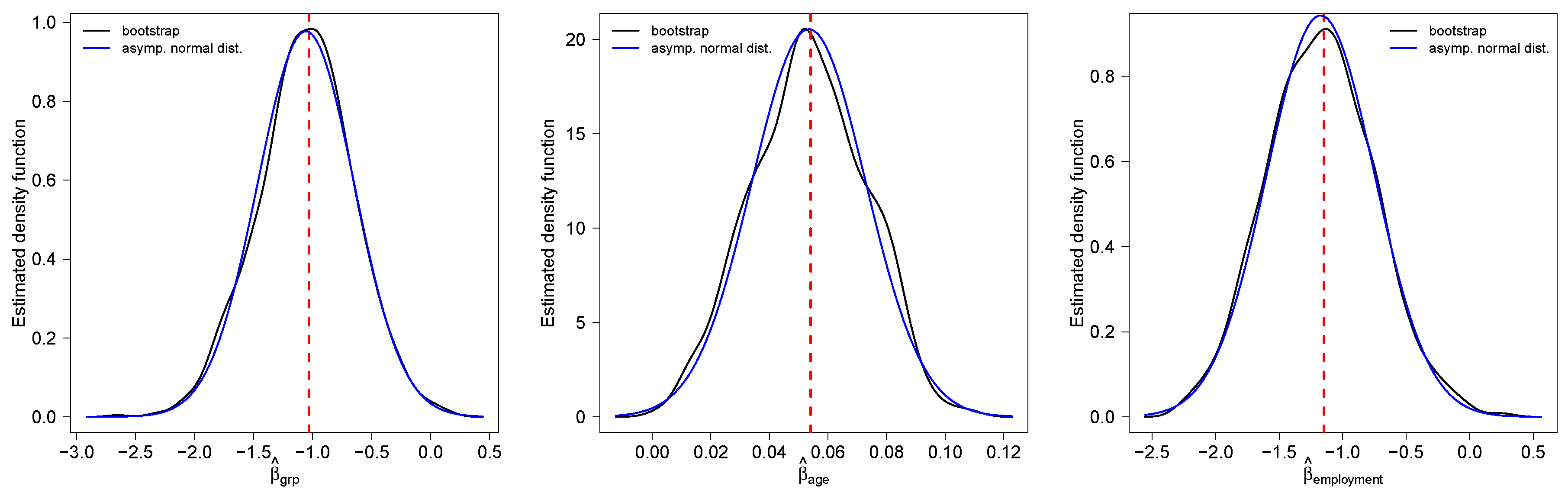
5.1. Smokers Dataset

This dataset is related to a clinical trial on the effectiveness of triple-combination pharmacotherapy for tobacco dependence treatment conducted by the Cancer Institute of New Jersey and Robert Wood Johnson Foundation. The trial recruited 127 smokers 18 years or older with predefined medical illnesses from the local community. The outcome were the time (in days) to first relapse (return to smoking). The study lasted 182 days (26 weeks). Therefore, the times are subject to a censoring type I (32% of times were censored). We only considered the 113 patients where such observed time was positive (non-zero). Other measures were assigned randomly treatment group with levels combination or patch only (grp), age in years at time of randomization (age) and employment (full-time or non-full-time). We consider that time${}_i\sim$WE$({\theta }_i;\sigma )$, where $log{\theta }_i={\mathit{X}}_i^{\top }\mathit{\beta }$, $\mathit{\beta }={({\beta }_{\mathtt{intercept}},{\beta }_{\mathtt{grp}},{\beta }_{\mathtt{age}},{\beta }_{\mathtt{employment}})}^{\top }$ and

$${\mathit{X}}_i^{\top }=(1,{\mathtt{grp}}_i,{\mathtt{age}}_i,{\mathtt{employment}}_i)$$

We estimated ${\widehat{\sigma }}_J=1.617008$ based on the jackknife method, which was used as known in all the computations.

Table 2. Estimates for parameters and skewness coefficient in smokers dataset.

Parameter	Estimate	s.e.	${\mathit{\gamma }}_1$
${\beta }_{\mathtt{intercept}}$	3.1690	0.8136	−0.0478
${\beta }_{\mathtt{grp}}$	−1.0303	0.3694	−0.0529
${\beta }_{\mathtt{age}}$	0.0541	0.0167	0.1251
${\beta }_{\mathtt{employment}}$	−1.1460	0.3935	−0.0753

shows the parameters estimates, their standard errors and the estimated skewness coefficients and Figure 1 shows the estimated density function based on 1000 bootstrap samples for the coefficients related to the covariates grp, age and employment. Note that the estimated skewness for all parameters were closer to zero, suggesting a symmetric distribution for the estimators which is corroborated by the estimated density based on the bootstrap.

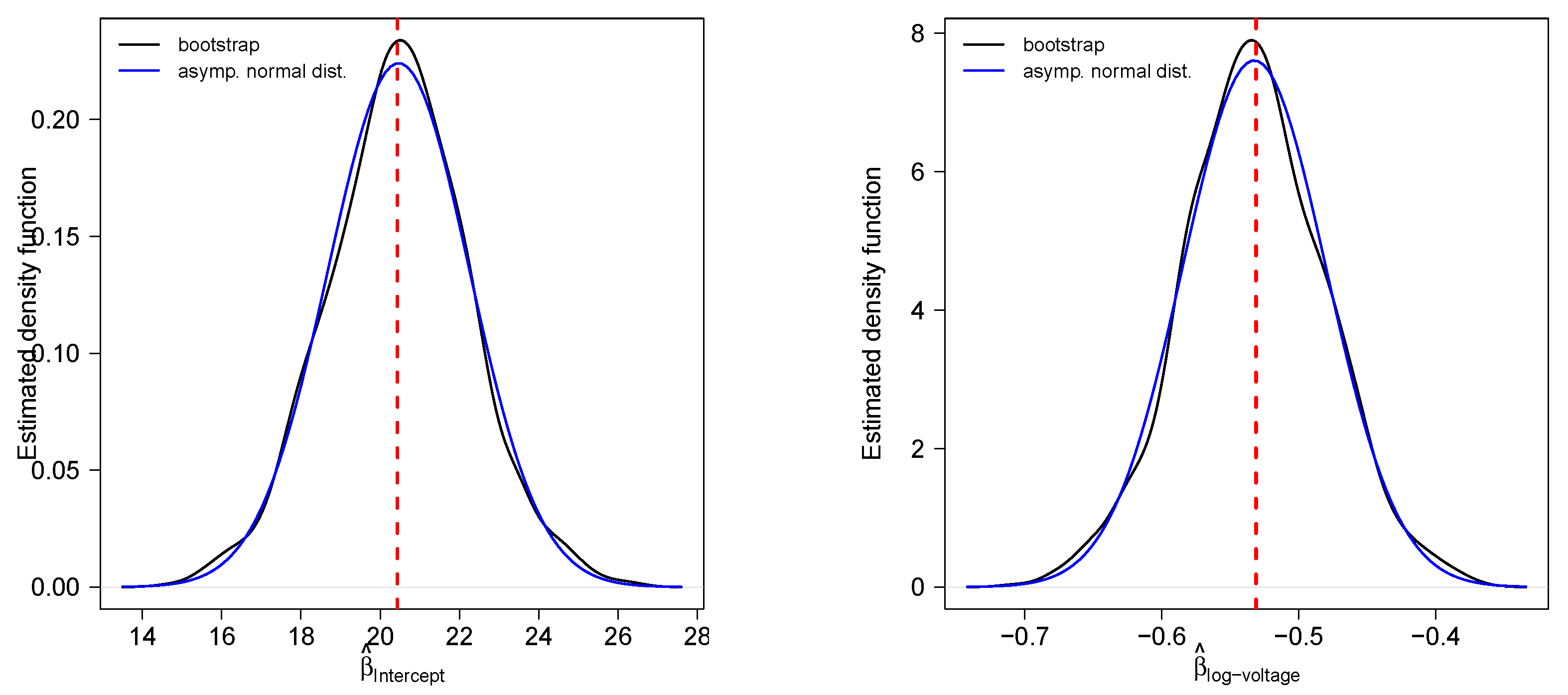
5.2. Insulating Fluids Dataset

This dataset was presented in [11] on insulating fluids and it is related an accelerated test performed in order to determine the relationship between time (in minutes) to breakdown and voltage (in kilovolts). The authors assumed a regression structure based on the Weibull model and a common censoring time at $L=200$ (type I censoring), i.e., time${}_i\sim$WEI$({\theta }_i,\sigma )$, where $log{\theta }_i={\mathit{X}}_i^{\top }\mathit{\beta }$, $i=1,\dots ,76$, ${\mathit{X}}_i^{\top }=({\beta }_{\mathtt{Intercept}},{\beta }_{\mathtt{log}}-\mathtt{voltage})$. We estimated ${\widehat{\sigma }}_J=1.296704$ based on the jackknife method, which was used as known.

Table 3. Estimates for parameters and skewness coefficient in insulating fluids dataset.

Parameter	Estimate	s.e.	${\mathit{\gamma }}_1$
${\beta }_{\mathtt{intercept}}$	20.4342	1.8772	0.1451
${\beta }_{\mathtt{log}}-\mathtt{voltage}$	−0.5311	0.0557	−0.1517

shows the estimates, standard errors and estimated skewness coefficient for the MLE estimators and Figure 2 shows the estimated density function for ${\widehat{\beta }}_{\mathtt{Intercept}}$ and ${\widehat{\beta }}_{\mathtt{log}}-\mathtt{voltage}$. Newly, the estimated skewness for both parameters are closer to zero, suggesting a symmetric distribution for the estimators as also suggest the estimated density based on bootstrap.

6. Concluding Remarks

Since its beginning, the Weibull distribution and regression showed how it is important. In the frequentist context, this model depends strongly on the asymptotic properties of the MLE. Here, we presented an expression of the skewness that, in practical applications, can be used as an indicator of departure from the normal distribution of the MLE. Although the expression (3) entails a great deal of algebra, the final expression (5) of the skewness of the MLE distribution has a very nice form only involving simple operations on diagonal matrices and can be easily implemented into a statistical software, for instance, R, [10].

References

1. Weibull, W. A statistical distribution function of wide applicability. J. Appl. Mech. 1951, 18, 293–297. [Google Scholar]
2. Kendall, M.G.; Stuart, A. The Advanced Theory of Statistic, 4th ed.; Griffin: London, UK, 1977. [Google Scholar]
3. Bowman, K.O.; Shenton, L.R. Asymptotic skewness and the distribution of maximum likelihood estimators. Commun. Stat. Theory Methods 1998, 27, 2743–2760. [Google Scholar] [CrossRef]
4. Cordeiro, H.H.; Cordeiro, G.M. Skewness for parameters in generalized linear models. Commun. Stat. Theory Methods 2001, 30, 1317–1334. [Google Scholar] [CrossRef]
5. Magalhães, T.M.; Botter, D.A.; Sandoval, M.C.; Pereira, G.H.A.; Cordeiro, G.M. Skewness of maximum likelihood estimators in the varying dispersion beta regression model. Commun. Stat. Theory Methods 2019, 48, 4250–4260. [Google Scholar] [CrossRef]
6. Cordeiro, G.M.; Colosimo, E.A. Improved likelihood ratio tests for exponential censored data. J. Stat. Comput. Sim. 1997, 56, 303–315. [Google Scholar] [CrossRef]
7. Cordeiro, G.M.; Colosimo, E.A. Corrected score tests for exponential censored data. Stat. Probab. Lett. 1999, 44, 365–373. [Google Scholar] [CrossRef]
8. Magalhães, T.M.; Gallardo, D.I. Bartlett and Bartlett-type corrections for Weibull censored data. Stat. Oper. Res. Trans. 2019. Submitted. [Google Scholar]
9. Lemonte, A.J. Non null asymptotic distribution of some criteria in censored exponential regression. Commun. Stat. Theory Methods 2014, 43, 3314–3328. [Google Scholar] [CrossRef]
10. R Development Core Team. A Language and Environment for Statistical Computing; R Foundation for Statistical Computing: Vienna, Austria, 2019. [Google Scholar]
11. Nelson, W.; Meeker, W.Q. Theory for optimum accelerated censored life tests for Weibull and extreme value distributions. Technometrics 1978, 20, 171–177. [Google Scholar] [CrossRef]
12. Renyi, A. On the theory of order statistics. Acta Math. Hung. 1953, 4, 191–231. [Google Scholar] [CrossRef]
13. Devianto, D.; Oktasari, L.; Maiyastri. Some properties of hypoexponential distribution with stabilizer constant. Appl. Math. Sci. 2015, 142, 7063–7070. [Google Scholar] [CrossRef]
Figure 1. Estimated density function based on 1000 bootstrap samples and the asymptotic distribution for β ^ grp (left panel), β ^ age (center panel) and β ^ employment (right panel). The red line denotes the estimated parameter.
Symmetry 11 01351 g001
Figure 2. Estimated density function based on 1000 bootstrap samples and the asymptotic distribution for β ^ Intercept (left panel) and β ^ log voltage (right panel). The red line denotes the estimated parameter.
Symmetry 11 01351 g002