Abstract
Abstractive text summarization that generates a summary by paraphrasing a long text remains an open significant problem for natural language processing. In this paper, we present an abstractive text summarization model, multi-layered attentional peephole convolutional LSTM (long short-term memory) (MAPCoL) that automatically generates a summary from a long text. We optimize parameters of MAPCoL using central composite design (CCD) in combination with the response surface methodology (RSM), which gives the highest accuracy in terms of summary generation. We record the accuracy of our model (MAPCoL) on a CNN/DailyMail dataset. We perform a comparative analysis of the accuracy of MAPCoL with that of the state-of-the-art models in different experimental settings. The MAPCoL also outperforms the traditional LSTM-based models in respect of semantic coherence in the output summary.
1. Introduction
At present, it is a challenging task to retrieve useful information from a large text due to the unseen growth of blogs, article, and reports. Here, an automated text summarization technique gives an effective solution to extract useful information from the large text. Text summarization is a task of condensing a text that keeps the actual meaning and important parts of the original text. A concise and quality summary assists humans in processing and understanding a large text in a short time. However, automatically summarizing a large text is still an open problem. There are two possible ways to perform text summarization: extractive and abstractive [1]. The process of copying words and sentences directly as a summary from the long text is called extractive summarization. Most of the conventional text summarization models are based on the extractive text summarization (ETS) technique. Those models are relatively simple and produce grammatically correct sentences while failing to generate a semantically coherent summary [2,3]. In contrast, abstractive text summarization, a relatively new concept, has drawn interest among the researchers because of its capability of generating new words using language generation models. Abstractive text summarization generates a summary by paraphrasing the text while it keeps the actual meaning in the summary text [4]. Extractive text summarization ensures syntactic structure but fails to guarantee the semantic coherence in the generated summary. On the other hand, the abstractive text summarization works effectively for maintaining semantic coherence while failing to ensure the syntactic structure of the generated summary [5].
The abstractive text summarization has great potential for generating a high-quality summary by using sequence-to-sequence (seq2seq) modeling [6]. Sequence-to-sequence modeling, a recurrent neural network model, takes a sequence of text as input and generates a sequence of text as output. The encoder–decoder architecture of the seq2seq model can be implemented by an RNN (recurrent neural network) framework called long short-term memory (LSTM) [7]. It is successfully applied to a variety of NLP (natural language processing)-based problems like machine translation, headline generation, text summarization, and speech recognition. The LSTM performs promisingly to produce a concise abstractive summary although it has some limitations. It does not allow for accessing the previous cell state when the output gate is closed. This problem is overcome by a variation of LSTM called Peephole Convolutional LSTM (PCLSTM) that performs efficiently in various types of classifications and predictions. The PCLSTM allows accessing the previous cell state even when the output gate is closed [8]. The more utilization of the previous memory cell content assists with capturing the full dependency that enhances the accuracy of a model. In this work, we develop an abstractive text summarization model using multi-layered attentional peephole convolutional LSTM.
The performance of a machine learning model highly depends on the optimization of the parameters of that model. The optimization of parameters is often carried out by the design of experiment (DoE). The fundamental purpose of the design of experiment is to understand the interaction among parameters, and optimize the parameters for getting the highest response. Traditionally, the parameter optimization is done using the conventional methods which do not consider the combined effect of parameters. Hence, the statistical methods of the design of experiment are used to optimize the parameters of a machine learning algorithm which eliminates the problems of the conventional methods. The design of experiment (DoE) has two phases—the first phase is to filter the most significant parameters, and the second phase is to optimize the parameters [9]. The central composite design (CCD) is widely used for performing the task of filtering. It reduces the number of parameters by performing statistical analysis, where it calculates the importance of each parameter to generate a better response [10]. The optimization of parameters is carried out by applying a response surface method (RSM). The RSM is a statistical method that uses experimental data to optimize a response that is influenced by independent input parameters.
The evaluation technique of a summary plays a significant role to decide the credibility of the summarization model. There are two types of evaluation techniques like intrinsic and extrinsic evaluation [11]. The intrinsic evaluation measures the quality of a summary by direct analysis based on some factors while the extrinsic evaluation evaluates a summary based on how it affects the completion of some other tasks [12]. The evaluation techniques based on recall, precision, and F-measure are called intrinsic evaluation. The intrinsic evaluation techniques like ROUGE (Recall-Oriented Understudy for Gisting Evaluation) [13] and BLEU [14] are widely used for judging the quality of a summary. In this paper, we have used the ROUGE method for measuring the quality of our model generated summary. The quality of a summary also depends on the level of difficulty of reading and understanding. Hence, readability metrics is also essential for judging the quality of a summary. There exist several techniques such as ARI (automatic readability index) [15], Flesch reading ease [16], etc. that use a simple linear equation with two or more language features like lexical and syntactic features to compute the readability metrics. The lexical feature decides the difficulty of a word while syntactic feature focuses on the difficulty of a sentence by averaging the sentence length [12]. The word difficulty is measured by computing the number of syllables in a word, number of characters in a word, and word frequency. In this paper, we have used ARI and Flesch reading ease techniques to measure the readability metrics.
In this paper, we develop an abstractive text summarization model (MAPCoL) using the peephole convolutional LSTM (PCLSTM) instead of the traditional LSTM. We add the attention strategy in the final layer of the model, which helps to select the important word as a summary. We also incorporate the multiple layers of PCLSTM which assist the model with capturing the complete pattern of training data. The addition of the multiple layers helps the model to generate syntactically and semantically coherent summary. The Keras with TensorFlow backend is used to implement the model. The developed model is also optimized using the central composite design (CCD) in combination with the response surface method (RSM). Additionally, the value of maximized output has been predicted using the RSM that has been justified by the experimental results later. We also perform a comparative analysis of the performance of our model in different internal settings with the abstractive state-of-the-art models.
The rest of the paper is organized as follows: Related works are discussed in Section 2. Section 3 illustrates the existing traditional LSTM-based model, and develops a peephole convolutional LSTM-based model and design of experiment (DoE) to optimize our proposed model. The experiment, data set, and evaluation approach are discussed in Section 4, while experimental results are discussed in Section 5. Section 6 illustrates the scope of future improvements of this work followed by some conclusive remarks.
2. Related Works
Abstractive text summarization has drawn special attention since it can generate some novel words using seq2seq modeling as a summary. Most of the research on text summarization in the past are based on extractive text summarization, while very few works have been done on abstractive text summarization. Some significant research on both of the summarization techniques is described below.
The neural network is widely used in the extractive text summarization (ETS). An ETS model using reinforcement learning was developed that considers the extractive summarization as a sentence ranking task [17]. They used a CNN-Daily mail data set and obtained a good result. A neural extractive text summarization model was described that can score and select sentences jointly [18]. An extractive model using a data-driven approach for text summarization was shown in [19]. They used a feedforward neural network to build the model. LeadR, a neural model for extractive summarization, produced a probability distribution over positions of sentences and used that probability to locate a sentence in a summary [20]. Few recent works on extractive text summarization generate summary in a more data-driven way. The attention strategy is also incorporated in the extractive summarization. A neural model with attention mechanism was introduced that focuses on the important parts of the text and used them as a summary [21]. SummaRuNNer, an ETS model based on a recurrent Neural Network (RNN) that produced a summary by considering content, salience, and novelty of the source text [22]. Recently, long short-term memory (LSTM) is applied to build the extractive summarization model. An LSTM-based neural model for ETS was developed that shows promising improvement in the quality of summary [23]. A comparative analysis was conducted that reveals the superiority of RNN-based extractive summarization over the traditional extractive summarization techniques [22].
Deep learning has a wide application in the abstractive text summarization (ATS). Abstractive summarization based on the attentive recurrent neural network works effectively for summary generation [24,25]. The RNN based ATS model generates a summary with a better ROUGE score. Another abstractive text summarization model based on the sequence-to-sequence modeling was developed [6] that uses GRU (Gated Recurrent Unit) with a bidirectional neural network for building the model. In recent works, the encoder–decoder seq2seq modeling of RNN is used to build the abstractive text summarization model. An abstractive summarization based on attentional encoder–decoder was implemented by using long short-term memory (LSTM) [26]. Another work using long short-term memory (LSTM) was proposed that uses both bidirectional or unidirectional encoder–decoders [27]. LSTM with a combination of convolutional neural network (CNN) returns better accuracy in the abstractive summarization. An abstractive summarization model named ATSDL was developed by blending LSTM with CNN that ensures both semantic coherence and syntactic structure of a sentence [28]. ATSDL takes phrases as input instead of raw text after identifying the phrase from the source text.
A variation of traditional LSTM called convolutional LSTM works effectively in different types of predictions and classifications. For precipitating nowcasting, a model based on convolutional LSTM (ConvLSTM) was developed by extending the fully connected (FC-LSTM) [29]. The developed ConvLSTM model considered the complete correlation among data and predicted nowcast with better accuracy than the traditional LSTM-based model. The convolutional LSTM was also used for time series classification. The model used a fully convolutional long short-term memory (LSTM) that classifies the time series very effectively [30]. Another work based convolutional long short-term memory (CNN-LSTM) was conducted for gas source localization using time series data from a gas sensor network and an anemometer [31]. The model performed well to find the location of a gas source despite having some challenges like inconsistent airflow and gas distribution in outdoor environments. A method based on CNN + Convolutional LSTM (ConvLSTM) was trained end to end for the tool presence detection, spatial localization, and motion tracking [32]. The convolutional LSTM is widely used in gesture recognition. A multimodal gesture recognition method based on 3D convolution and a convolutional long-short-term-memory-based model developed for gesture recognition [33]. They used ConvLSTM to learn the long-term spatiotemporal features that help to achieve 98.89% recognition accuracy. The aforementioned convolutional LSTM-based models perform better than the models based on traditional LSTM. The architecture of convolutional LSTM allows the model to consider the full dependency of time stamp during model training. Since the convolutional LSTM works effectively in various classifications and predictions, it will also do well in the abstractive text summarization. The convolutional LSTM network with extra peephole connection will give better accuracy than the traditional LSTM network.
The parameter optimization is widely used in machine learning. The performance of a machine learning model is significantly influenced by the parameter optimization. A machine learning model was optimized by using the design of experiment (DoE) [9]. They used factorial design to filter the most significant parameters, and RSM to optimize the parameters. The response surface method was applied [34] for the optimization of leaching parameters for ash reduction from low-grade coal. Their optimized model produced better accuracy than the conventional one. An artificial neural network-based model for accessing the optimum bio-diesel and diesel was optimized by using the response surface method [10]. Their experimental results indicate that the parameter optimization affects the performance greatly. However, the optimization by the response surface method has been used in different fields of research while it is not yet used to optimize the text summarization model.
All the aforementioned works on abstractive text summarization are based on traditional LSTM. However, the traditional LSTM has some limitations, such as it does not allow for accessing the previous cell state when the output gate is closed. The performance of a model can be improved using parameter optimization. However, parameter optimization is rarely used in conventional models, if not any. Hence, we have introduced a variation of the traditional LSTM called peephole convolutional LSTM to build an abstractive summarization model. We have optimized our developed model using the design of experiment method injunction with the response surface method that returns better results in terms of semantic coherence than the existing models that are based on the traditional LSTM architectures.
3. Abstractive Text Summarization Models
The goal of this study is to develop an abstractive text summarization model using a variation of long short-term memory (LSTM) called peephole convolutional LSTM. Since the common form of LSTM called traditional LSTM has some limitations like dependencies among cells not being strong [29,35], the peephole convolutional LSTM is used to build the model instead of the traditional LSTM. In this section, the traditional LSTM and the peephole convolutional LSTM are explained in detail.
3.1. Traditional LSTM Unit
The long short-term memory (LSTM) is a unit of a recurrent neural network that can identify and remember the data pattern for a certain period. The LSTM takes a sequence of text as input and predicts a sequence of text as output. It consists of a memory cell, an input gate, an output gate, and a forget gate. These three gates control the memory content and the cell states at the current timestamp [36]. The architecture of traditional LSTM unit is shown in Figure 1.
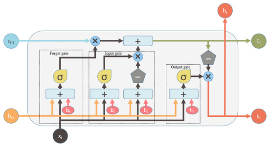
Figure 1.
A traditional LSTM (long short-term memory) with three gates: input, forget, and output gates. The content of the memory block is controlled by these three gates. Here, and are respectively the contents of the previous and the current memory cells, and are respectively the outputs of the previous and the current states, is an input vector, X is a bitwise multiplication, + is a bitwise summation, is a hyperbolic tangent function, is a sigmoid function. , , , and are the bias of the different gates.
Here, the top line is known as a memory pipe that takes previous memory content as input and generates final memory as output. The previous memory content is passed under two different operations: bitwise multiplication (x) with the output of the forget gate and bitwise summation (+) with the output of the input gate. The forget gate generates an output within the range 0 to 1, which plays an important role in deciding the content of the memory at the current timestamp. The output close to 0 means that most of the previous memory content will nearly be forgotten and the opposite will happen for the output near to 1. The bitwise summation (+) of the output of the input gate determines how much input from the current timestamp will be added to the previous memory content to produce the final memory at the current timestamp. Here, the input gate also produces an output within the range 0 to 1.
The forget gate takes the output of the previous state , an input vector , and a bias as input and generates a value within range 0 to 1 that decides how much content of the memory will pass through the memory pipe:
The input gate also generates a value within 0 to 1 that defines how much input from the current timestamp will add to the memory content at the current timestamp:
The output gate takes the content of the previous state, an input vector , and a bias as input and produces as output. Finally, the content of the current state is produced using the value of :
In the architecture of the traditional LSTM, there is no connection between a gate and its previous memory cell. This is why it is not possible to access the previous memory cell state when the output gate is closed, and it is often found closed during training. A variation of LSTM, called peephole convolutional LSTM, can overcome this problem.
3.2. Peephole Convolutional LSTM Unit
Long short-term memory (LSTM) is a recurrent neural network unit that has wide applications in sequence prediction problems. A common form of LSTM, known as traditional LSTM, can not access the content of its previous memory cell when its output gate is closed [29]. By adding an extra connection between each gate and the previous memory content, we can solve this problem of the traditional LSTM. This additional connection, known as a peephole connection, allows all of the gates to utilize the previous memory cell content even when the output gate is closed. The architecture of peephole convolutional LSTM is shown in Figure 2.
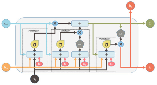
Figure 2.
A peephole convolutional LSTM with a peephole connection. Here, each gate is connected with the content of the previous memory cell . The memory of the previous cell along with , , and bias are provided as input to each gate. This allows for accessing the content of the previous memory cell even when the output gate is closed.
The implementation of peephole convolutional LSTM is as follows:
Here, the previous memory cell content along with other parameters are provided as input in the peephole convolutional LSTM while the traditional LSTM does not consider as input. Taking as input in the peephole convolutional LSTM influences the result of the sequence prediction problem. Therefore, we apply the peephole convolutional LSTM for abstractive summarization.
3.3. MAPCoL Model
The goal of this study is to develop an abstractive summarization model using multi-layered attentional peephole convolutional LSTM (MAPCoL).
Figure 3 shows the working process of the MAPCoL model. We add multiple layers of PCLSTM in MAPCoL, which means it has more than one hidden layer. We use two hidden layers to build the model since a layer size of more than three drops the performance of the model due to the gradient decay over the layers. Initially, the given input text is passed through the embedding layer that converts the given text into numerical distributed representations. These representations are passed through two hidden layers of PCLSTM, each layer with a hundred hidden units. Here, the encoder and the decoder of seq2seq modeling works. The encoder captures the feature vector that represents the given text. At the same time, it calculates the attention weight for each given word and stores it in an attention vector that has been used to generate a precise summary in the dense layer. Here, the attention weight is also calculated for each word and stored in the same attention vector. The attention strategy helps the sequence-to-sequence model to remember important aspects of a given input [27]. The attention weight of an input word at position t is computed when outputting the word as follows:
where represents the last hidden layer generated after processing input word, and represents the last hidden layer generated from the current step of decoding. The attention mechanism calculates the conditional probability of an input word. Once the entire given text is passed through the encoder, the decoder takes the feature vector from the encoder and generates the best text for the intended summary. The decoder generated text is passed through a final dense layer that utilizes the attention vector to select the most important parts as a final summary.
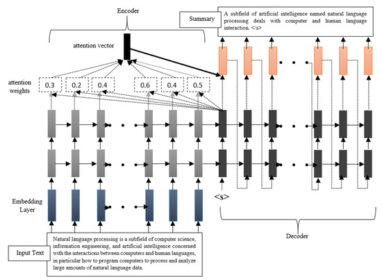
Figure 3.
The entire work flow of the model which starts by taking an input text and finishes by generating a summary.
We apply our developed MAPCoL model on CNN-Daily Mail data set. The system summary and the reference summary are shown in Table 1.

Table 1.
Comparison of system summary and reference summary.
Table 1 shows that the system summary looks better than the reference summary in terms of syntactic and semantic coherence.
The second phase of this study is to optimize the developed model using the central composite design (CCD) along with the response surface method (RSM). The model is optimized based on four parameters like epochNumber, batchSize, learningRate and hiddenUnits. A total number of 30 experiments is conducted in order to build a data set for optimization. The experiment for the optimization is built using the CCD. Then, RSM is used to perform the final optimization. RSM generates a quadratic polynomial equation based on the result of ANOVA analysis. Using that polynomial equation, RSM predicts the optimal output for the designated model.
3.4. Design of Experiment (DoE)
The parameters used for training and testing the developed model are needed to optimize to improve the performance of the model. In this study, the parameters of the developed model are optimized to improve the model performance using the central composite design (CCD) in combination with the response surface methodology (RSM). The RSM is a combination of mathematical and statistical methods that is used for building an empirical model to improve and optimize the parameters. It also investigates the combined effects of interaction among the parameters.
The central composite design is introduced to determine the number of experiments needed to optimize the variables and response. The CCD is also incorporated to filter the significant parameters from the candidate parameters. Additionally, the experimental design for performing the optimization is built by using the CCD. The CCD has three parts— factorial points coded to +1 to –1 notation, axial points (± a, 0, 0 ... 0), (0, ± a, 0 ... 0) ... (0, 0, ± a ... 0), and center points (0, 0, 0 ... 0). The vertices of the n-dimensional cube that are coming from the full or fractional factorial design are called fractional points. The center point is located at the center of the design space. The points on the axes of the coordinate system with respect to the central point at a distance of from the design center are called axial point. The total number of experiments required for an n-factor of a three-level CCD is , where n is the number of independent variables, is the corner points of the cube representing the experimental domain, is the axial points while is the center point that represents the replication of the test. The total number of experiments for the designed CCD with four factors of three-level and six replications of the test is . After designing the experimental model by the CCD, the response surface methodology is applied for the final optimization.
The RSM, which is used to optimize the variables as well as the response, has three phases—design of experiment space, determination of coefficient, and prediction of response with optimized variables. In this study, four independent variables are used for the experiment: epochNumber (), batchSize (), learningRate (), and hiddenUnits (). The range of values of these parameters is varied depending on the experiments. The results of different experiments with parameters are used to perform the optimization. The interaction among response and independent variables is as follows:
where Y is the response and is the independent variable of the system. The primary purpose of the design of experiment (DoE) is to optimize the response variable. Hence, it is necessary to determine a statistical correlation between the response variable and the independent variables. An analysis of variance (ANOVA) is carried out for graphical analysis of data that finds the correlation between the response surface and the independent variables. The values of P and F tests define the statistical significance of a variable over the response. An empirical model is built using the response to correlate the independent variables by generating a quadratic polynomial equation:
where Y, , , , and are respectively the predicted response variable, the constant coefficient, the linear coefficient, the quadratic coefficient, and the interaction coefficient. Additionally, n number of parameters are examined and optimized; , are the coded value of the parameters; and is the random error. The coded value of the parameter is calculated as follows [34]:
Here, the coded independent variable is , is the uncoded independent variable, and is the uncoded independent variable at the centre point. The accuracy of the quadratic polynomial equation is determined by the value of while the significance of the model is evaluated by the probability value (p-value) at a 95% confidence level. The optimization is carried out by a statistical software package Design Expert, Stat-Ease, Inc., Minneapolis, MN, USA. This software package is also used to plot the contour plot and the response surface plot in the optimized condition.
4. Experiment
The study is aimed to develop an abstractive text summarization with the help of peephole convolutional LSTM. We optimize the parameters of our MAPCoL model using the central composite design (CCD) in combination with the response surface methodology (RSM).
4.1. Experimental Setup
To develop a peephole convolutional LSTM-based abstractive text summarization model, we have used Python libraries Keras with a TensorFlow CPU backend. The batch size defines that the amount of data are used at a time while training a model. The epoch number means how many times data are used to train a model. We keep the batch size of 64, and the number of epochs of 200, to train our MAPCoL model. Our model with this setting produces the best result in terms of semantic coherence as well as syntactic structure. Then, we use a software called design expert to perform the optimization.
4.2. Experimental Data Set
Our experiment for generating a summary using multi-layered attentional peephole convolutional LSTM is carried out on the CNN-Daily Mail data set. The data set contains online news articles and a summary of those news articles. Here, the used dataset contains 287,226 training pairs, 13,368 validation pairs, and 11,490 testing pairs.
4.3. Evaluation Method
Manual evaluation of the quality of a summary is time hungry, annoying, and repetitive [37]. Hence, a method called ROUGE (Recall-Oriented Understudy for Gisting Evaluation) is used for summary evaluation [38] that evaluates the quality of a summary by comparing a system summary and a reference summary (human-generated). Different approaches are followed to measure ROUGE scores. In this study, we use ROUGE-N [13] and ROUGE-L [13] to evaluate the quality of our model generated summary. ROUGE-N is a recall oriented evaluation method that measures the quality of a candidate summary against a reference summary by considering n-gram. The ROUGE-N is measured as follows [13]:
where n is the number of consecutive words, is the set of reference summary, counts the number of n consecutive words of the reference summary, and counts the number of matched n consecutive words between the reference summary and system summary.
Another ROUGE method called ROUGE-L evaluates the quality by taking the longest common subsequence (LCS) between a candidate summary and a reference summary into consideration. The F-measure based ROUGE-L is estimated as follows [13]:
Here, and are the LCS-based recall and precision, respectively, while .
Another evaluation method called readability metrics is performed to evaluate the quality of a summary. Readability metrics are the techniques for judging the reading difficulty of a text by considering the letters, words, and sentences. Readability score defines the level of difficulty of a particular text. The following techniques are widely used to calculate the readability metrics.
The Automated Readability Index (ARI) [15] outputs a number that indicates the age needed to understand the text [15]:
The Flesch Reading Ease formula defines how easy or difficult a text is to read [16]. The Flesch Reading Ease score is between 0 to 100, and a higher number means that it is easier to read [16]:
where ASL = average sentence length (number of words divided by the number of sentences) and AWL = average word length in syllables (the number of syllables divided by the number of words).
5. Results and Discussion
The peephole convolutional LSTM works efficiently in different types of classifications and predictions. In this paper, we introduce a multi-layered attentional peephole convolutional LSTM to build an abstractive text summarization model (MAPCoL). In addition, we optimize the model to get better output using the central composite design (CCD) in combination with the response surface method (RSM).
5.1. Summary Generation by MAPCoL
We apply our model on a popular CNN/Daily Mail data set, and compare this result with that of the other models applied over the same data set, as shown in Table 2. We have calculated ROUGE-1, ROUGE-2, and ROUGE-L scores to evaluate the performance of our model. Here, ROUGE-1 measures summary quality by considering a single word while ROUGE-2 by considering two consecutive words at a time.
Table 2.
Performance comparison between the MAPCoL and other models on the CNN/DailyMail dataset. ROUGE stands for Recall-Oriented Understudy for Gisting Evaluation.
Table 2 shows the ROUGE scores that are obtained by four different text summarization models. The models shown in Table 2 obtain this result on the same CNN/Daily Mail data set. Here, the three models shown, such as Bottom-Up Sum [39], SummaRuNNer [22], and C2F + ALTERNATE [6], are based on a recurrent neural network (traditional LSTM), while our MAPCoL model is based on peephole convolutional LSTM. The highest ROUGE-1, ROUGE-2, and ROUGE-L scores obtained by the traditional LSTM-based models mentioned in Table 2 are 41.22, 18.68, and 38.34%, respectively. In contrast, the peephole convolutional LSTM-based model (MAPCoL) achieves ROUGE-1, ROUGE-2, and ROUGE-L scores 39.61, 20.87, and 39.33 percent, respectively, which are higher than that of the traditional LSTM-based model except for the ROUGE-1 score.
The model generates summary with more accuracy after optimization and the improved ROUGE-1, ROUGE-2, and ROUGE-L are 41.21, 21.30, and 39.42%, respectively. The ROUGE-1 of our model is very close to ROUGE-1 of the Bottom-Up Sum model while the other two ROUGE scores are greater than that of the comparing three models. The reason behind the better performance of our MAPCoL model is the peephole connection in LSTM architecture that allows us to access the cell state in any condition. Additionally, the multi-layered topology of LSTM in encoder–decoder architecture influences the performance improvement of our model.
The readability of our model generated summary is also calculated. Here, two techniques such as automated readability index (ARI) [15] and Flesch reading ease [16] are used for measuring the level of difficulty of the model generated summary. The both techniques use the average word and sentence length to calculate the difficulty. Table 3 shows the statistics of a dataset that is used for the readability computation. Here, a total of 11,490 summaries are evaluated, and two features like AWL (average word length) and ASL (average sentence length) are used to measure reading and understanding difficulties. The readability metrics of our model generated summary is shown in Table 4.
Table 3.
Statistics of the dataset used for readability metrics.
Table 4.
Readability metrics of our model generated summary before and after optimization.
We have estimated the readability metrics of both summaries before and after optimization. Table 4 indicates that the readability metrics of the optimized and non-optimized summary are not varied significantly. The ARI score of 10.60 and 10.40 are respectively obtained from the summary of the optimized and non-optimized models which indicate that the generated summary is understandable for people in the 8th grade. Students who are below 8th grade will find this summary a little difficult to read and understand. The lower the Flesch score, the more difficult the text is to read. The estimated Flesch scores from the summary of the optimized and non-optimized models are 73.16 and 73.68, which means that the text is readable for the people of 7th or 8th grade students. The Krippendorff’s alpha test is used to measure the score of agreement between the two evaluators like ARI and Flesch reading ease score. The Krippendorff’s alpha is statistics the computes the agreement obtained among evaluators who evaluate a set of objects in terms of the values of the variables. To perform the Krippendorff’s alpha test, the ARI and Flesch scores are mapped to grade level by following Table 5. The ARI and Flesch scores of 11,490 summaries are mapped to the corresponding grade level using Table 5, and the Krippendorff alpha test is performed. This statistical test produced value of 0.8132, which indicates that the two observers agreed at 81.32% to score the readability of summaries.
Table 5.
ARI and flesch score mapping to the grade level.
We have performed some comparative analysis within our model by tuning different internal parameters. We have observed the performance of our model by changing the size of hidden units. We have experimented over the number of hidden units within the range 50 to 150, as shown in Figure 4. The performance of the model increases sharply with the increase in the size of hidden units from 50 to 100. More than 100 hidden units causes over-fitting that leads the model to memorize the given data instead of learning the data pattern. Hence, the model generalizes the unseen data less efficiently. However, increasing the size of hidden units to over 100 does not have any significant impact on the performance of this model. Additionally, it takes more time to finish the training. Hence, the size of hidden units being 100 is suitable based on performance and time consumption.
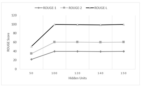
Figure 4.
Average performance of our MAPCoL with different numbers of hidden units.
We have also tested our model on different batch sizes. The batch size determines the amount of data used at a time to train the model. Here, we have tested the performance of MAPCoL on three different batch sizes keeping the size of hidden unit consistent at 100. The three different batch sizes are 32, 64, and 128. The performance of our model is very low with the batch size of 32, as shown in Figure 5.
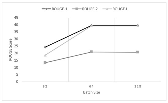
Figure 5.
Average performance of our developed MAPCoL on different batch sizes.
The performance increases rapidly until the batch size of 64 and then flattens out. The reason behind this is that the large batch size tends to converge to sharp minimizers of the training function. This tendency lessens the generalization power of the model and also reduces the ability to treat the unseen data precisely. Hence, the batch size of more than 64 has a diverse effect on the performance of the model. However, increasing the batch size also kills the overall training time. Hence, the use of batch size 64 against the unit size 100 shows the best result in our experiment.
We have also measured the ROUGE score with different epoch numbers, as shown in Figure 6. Here, the epoch number defines how many times the same data are used to train the model. In our experiment, the number of epochs varies from 100 to 250.
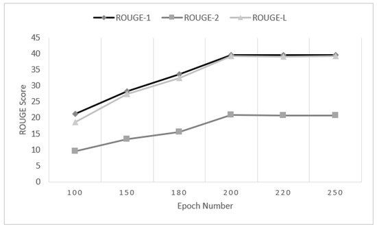
Figure 6.
Average performance of our MAPCoL model on different epoch numbers.
The performance of MAPCoL increases with the increase of epoch number. However, the performance improvement from 100 epochs to 200 epochs is very sharp, and this becomes stable afterward. Here, the over-fitting problem also occurred when the epoch number is more than 200. This is why the performance of the model is not improved when the model is trained for more than 200 epochs.
In our experiment, we also measure the training and validation accuracy of MAPCoL with respect to epoch numbers, as shown in Figure 7. A goal of building a model is to maximize the training and validation accuracy. Initially, the accuracy is low, and then it improves with the increase of epoch numbers. The accuracy of training and validation is falling after 200 epochs. This is because the model is facing the over-fitting problem after 200 epochs. Hence, both accuracies are falling after 200 epochs.
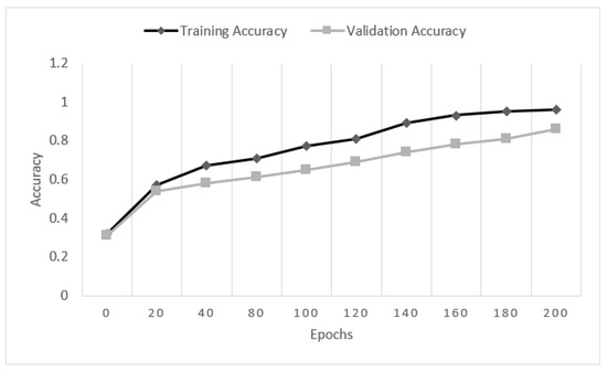
Figure 7.
Comparison of training and validation accuracy with epoch numbers.
Another expectation of building a deep learning model is that the training and validation loss will be near zero. The calculated validation and training loss with respect to the epoch number are shown in Figure 8. Figure 8 shows that both losses are decreasing as expected to epoch number 200 and, after that, they start increasing sharply. The reason for this unusual behavior is over-fitting, which puts a negative impact on the performance of the model.
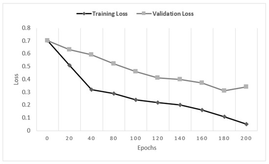
Figure 8.
Comparison of training and validation loss with epoch numbers.
The above experiments justify that our model MAPCoL produces better results than the state-of-the-art models of abstractive text summarization concerning semantic and syntactic structure.
5.2. Model Optimization by DoE
Model optimization is an important part of this study. The Design Expert software package is used to perform the regression analysis of the experimental data. The response surface plot is also drawn by this software package to investigate the combined effect of the parameters on the response variable. The values of the parameters used in optimization are chosen after performing a series of experiments. The model generates better results when the values of the parameters lie between the considered ranges.
A total number of 30 experiments with a different configuration of parameters are used to optimize the model. We have optimized the response variables such as ROUGE-1, ROUGE-2, and ROUGE-L concerning four important parameters of our model like epochNumber (), batchSize (), learningRate (), and hiddenUnits (). Table 6 shows the actual and coded value of four parameters along with the ROUGE scores in each of 30 experiments. These values are used to predict the maximum ROUGE scores along with the best configuration of these aforementioned four parameters to achieve that ROUGE score.
Table 6.
The coded and real value of the parameters along with response variable.
The statistical significance of each parameter over the response is evaluated by ANOVA analysis. The results of ANOVA for optimizing ROUGE-1, ROUGE-2, and ROUGE-l are shown in Table 7, Table 8 and Table 9, respectively.
Table 7.
Results of analysis of variance (ANOVA) for response surface in order to optimize the ROUGE-1.
Table 8.
Results of analysis of variance (ANOVA) for response surface in order to optimize the ROUGE-2.
Table 9.
Results of analysis of variance (ANOVA) for response surface in order to optimize the ROUGE-L.
The level of significance of each parameter is defined based on the F-value or p-value at a 95% confidence level. The larger F-value or the smaller p-value determine that the parameter is significant while the smaller F-value or the larger p-value indicate that the parameter is not significant. The parameters with p-values less than 0.05 are significant. Table 7 shows that , , , , and are statistically significant with respect to ROUGE-1. Table 8, the ANOVA results for optimizing ROUGE-2, shows that , , , , , and have significant impact on ROUGE-2. The optimization process is also carried out for ROUGE-L, and the ANOVA results in this regard are shown in Table 9.
Table 9 indicates that , , , , , , and have significant effects on ROUGE-L optimization. Here, the sum of square and mean of square define the variance between the individual value and the mean. The statistical parameters obtained from the ANOVA test to optimize ROUGE-1, ROUGE-2, and ROUGE-l are shown in Table 10, Table 11 and Table 12, respectively.
Table 10.
Statistical parameter obtained from the analysis of variance (ANOVA) for the ROUGE-1 optimization.
Table 11.
Statistical parameter obtained from the analysis of variance (ANOVA) for the ROUGE-2 optimization.
Table 12.
Statistical parameter obtained from the analysis of variance (ANOVA) for the ROUGE-L optimization.
The value of R-sq describes how perfectly the model has estimated the experimental data while R-sq(adj) adjusts the statistic based on the number of independent variables in the model. The R-sq(pred) indicates how well a model can predict the response for a new observation. A model with larger R-square value is better to optimize the output. The value of R-square, adjusted R-square, and predicted R-square for optimizing ROUGE-1 are 97.11%, 93.96%, and 90.90%, respectively. Table 10 shows that the model can estimate the experimental data with 97.11% accuracy. In addition, it can adjust the statistical data with 93.96% accuracy based on the independent variable. Table 10 also shows that, with 90.90% accuracy, the model can predict the best ROUGE-1 score.
Table 11 and Table 12 respectively show that the model can predict the optimum ROUGE-2 score with 91.14% and ROUGE-L score with 92.01% accuracy. An important step of response surface methodology is to perform the multiple regression analysis. The multiple regression analysis of the experimental data generates a quadratic polynomial equation for predicting the response variables such as ROUGE-1, ROUGE-2, and ROUGE-L. The quadratic equations obtained using response surface methodology are shown below:
This quadratic polynomial equation is used to predict the optimum value of the response variables. The predicted maximum ROUGE values with the optimal condition are shown in Table 13.
Table 13.
Predicted and experimental ROUGE scores with the optimal processing condition. Here, the star (*) sign represents the ROUGE scores getting through an experiment with the optimal values of the four parameters. The ROUGE scores without the star (*) sign are the predicted ROUGE scores by the optimization model.
Here, the values without star (*) sign are the predicted values by the response surface methodology while the values with star (*) sign are the experimental values using the best configuration of the four parameters. In this experiment, the response surface method (RSM) predicts the best ROUGE-1, ROUGE-2, and ROUGE-L scores of 41.98%, 21.67%, and 39.84% respectively with the best parameter configuration like epochNumber, batchSize, learningRate, and hiddenUnits are 200, 75.63, 0.001, and 111, respectively.
BY using the suggested parameter configuration by RSM, we found ROUGE-1, ROUGE-2, and ROUGE-L scores of 41.21%, 21.30%, and 39.42%, respectively, which is very close to the predicted ROUGE scores. Table 13 shows that the model gives a better result after optimization. This is because the value of the parameters is determined after considering the effect of the parameters on the response variable. The response surface method suggests the optimized values of the parameters after performing the multiple regression analysis. Hence, the optimized value of the parameters influences the ROUGE score significantly.
The response surface method is used to optimize the ROUGE scores and to examine the interaction of the parameters of the MAPCoL model. The level of significance of each parameter is investigated by performing the ANOVA test on the experimental data. Table 7, Table 8 and Table 9 show that the four parameters of the model have a significant influence on the ROUGE score. Here, to observe the combined effect of these parameters on the ROUGE score, the response surface methodology is used to draw the three-dimensional surface plot. Figure 9, Figure 10, Figure 11, Figure 12, Figure 13 and Figure 14 show the combined effect of epochNumber, batchSize, learningRate, and hiddenUnits on the ROUGE score.
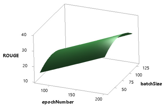
Figure 9.
Combined effect of epochNumber and batchSize on the ROUGE score.
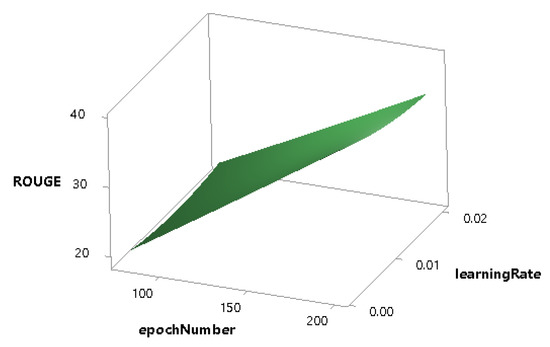
Figure 10.
Combined effect of epochNumber and learningRate on the ROUGE score.
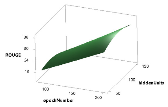
Figure 11.
Combined effect of epochNumber and hiddenUnits on the ROUGE score.
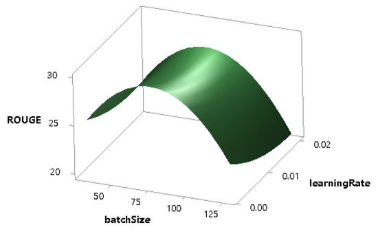
Figure 12.
Combined effect of batchSize and learningRate on the ROUGE score.
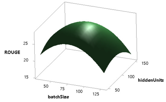
Figure 13.
Combined effect of batchSize and hiddenUnits on the ROUGE score.
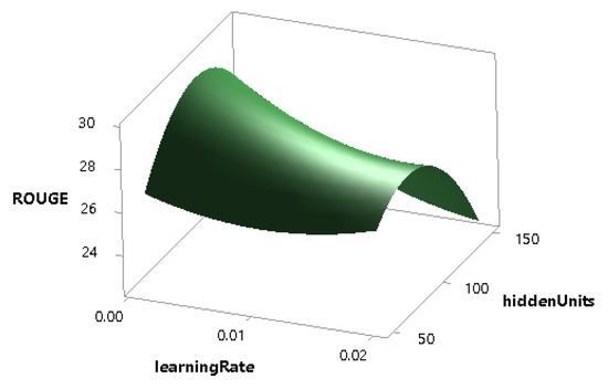
Figure 14.
Combined effect of learningRate and hiddenUnits on the ROUGE score.
Figure 9 shows that, with the increase of epochNumber, the ROUGE score increases linearly, and the model returns the maximum ROUGE score when the epochNumber is 200 and the batchSize is between 50 to 125.
Figure 10 defines that the ROUGE score grows sharply with the increase of epochNumber while the learningRate does not have a significant effect on the ROUGE score. The combined effect of the epochNumber and the hiddenUnits is shown in Figure 11, which indicates that the performance of the model increases linearly with the increase of epochNumber, but the hiddenUnits is less significant in this regard.
The effect of batchSize on the performance of the model is more than the learningRate as shown in Figure 12. Figure 13 shows that the batchSize and the hiddenUnits both have a significant combined impact on the performance, and, similarly, the learningRate and the hiddenUnits also have a notable combined effect on that of the model as shown in Figure 14.
The above experiments justify that our model MAPCoL produces better results shown in Table 2 than the state-of-the-art models of abstractive text summarization with respect to semantic and syntactic structure. Additionally, the optimized model has generated better accuracy than the un-optimized results. It is also seen that the model generates a more precise summary after optimizing the model using the response surface method.
6. Conclusions
The developed abstractive summarization model using multi-layered peephole convolutional LSTM achieves better performance than any state-of-the-art model with respect to semantic and syntactic coherence. The developed model has been optimized using the central composite design in combination with response surface design. The predicted ROUGE-1, ROUGE-2, and ROUGE-L scores found by the response surface method are 41.98%, 21.67%, and 39.84%, which are very close to the experimental of 41.21%, 21.30%, and 39.42%, respectively. The developed MAPCoL model overcomes some problems that are associated with the existing abstractive text summarization techniques. The semantic and syntactic coherence is also guaranteed in our developed model. Though our model overcomes some problems of other models, it also has some limitations. Our model works less efficiently when we generate a large text as a summary. In the future, we will work on that issue to make our model more efficient in order to generate a long summary. We have applied the developed model on the CNN-Daily Mail data set, and the MAPCoL works better than the traditional LSTM-based models.
Author Contributions
Conceptualization, M.M.R. and F.H.S.; methodology, M.M.R.; investigation, M.M.R.; Visualization, M.M.R.; Validation, F.H.S.; Writing—original draft preparation, M.M.R; supervision, F.H.S.; Writing-review and editing, F.H.S.
Acknowledgments
The authors are grateful to the Department of Computer Science and Engineering, Dhaka University of Engineering & Technology for providing us a opportunity to carry out this research.
Conflicts of Interest
There is no conflict of interest with the concerned persons or organizations.
Abbreviations
The following abbreviations are used in this manuscript:
| LSTM | Long Short-term Memory |
| PCLSTM | Peephole Convolutional Long Short-term Memory |
| DoE | Design of Experiment |
| CCD | Central Composite Design |
| RSM | Response Surface Method |
References
- Chen, J.; Zhuge, H. Abstractive Text-Image Summarization Using Multi-Modal Attentional Hierarchical RNN. In Proceedings of the 2018 Conference on Empirical Methods in Natural Language Processing; Association for Computational Linguistics: Brussels, Belgium, 2018; pp. 4046–4056. [Google Scholar]
- Yogatama, D.; Liu, F.; Smith, N. Extractive Summarization by Maximizing Semantic Volume. In Proceedings of the 2015 Conference on Empirical Methods in Natural Language Processing; Association for Computational Linguistics: Lisbon, Portugal, 2015; pp. 1961–1966. [Google Scholar]
- Mehta, P. From Extractive to Abstractive Summarization: A Journey. In Proceedings of the ACL 2016 Student Research Workshop; Association for Computational Linguistics: Berlin, Germany, 2016; pp. 100–106. [Google Scholar]
- Li, P.; Lam, W.; Bing, L.; Wang, Z. Deep Recurrent Generative Decoder for Abstractive Text Summarization. In Proceedings of the 2017 Conference on Empirical Methods in Natural Language Processing; Association for Computational Linguistics: Copenhagen, Denmark, 2017; pp. 2091–2100. [Google Scholar]
- Cheng, J.; Lapata, M. Neural Summarization by Extracting Sentences and Words. In Proceedings of the 54th Annual Meeting of the Association for Computational Linguistics; Association for Computational Linguistics: Berlin, Germany, 2016; Volume 1, pp. 484–494. [Google Scholar]
- Nallapati, R.; Zhou, B.; Santos, C.; Gulcehre, C.; Xiang, B. Abstractive text summarization using sequence-to-sequence rnns and beyond. In Proceedings of The 20th SIGNLL Conference on Computational Natural Language Learning; Association for Computational Linguistics: Berlin, Germany, 2016; pp. 280–290. [Google Scholar]
- Zhang, Y.; Liu, Q.; Song, L. Sentence-State LSTM for Text Representation. In Proceedings of the 56th Annual Meeting of the Association for Computational Linguistics; Association for Computational Linguistics: Melbourne, Australia, 2018; Volume 1, pp. 317–327. [Google Scholar]
- Gers, F.; Schraudolph, N.; Schmidhuber, J. Learning precise timing with LSTM recurrent networks. J. Mach. Learn. Res. 2003, 3, 115–143. [Google Scholar]
- Lujan, G.; Howard, P.; Rojas, O.; Montgomery, D. Design of experiments and response surface methodology to tune machine learning hyperparameters, with a random forest case-study. Expert Syst. Appl. 2018, 109, 195–205. [Google Scholar] [CrossRef]
- Najafi, B.; Ardabili, S.; Mosavi, A.; Shamshirband, S.; Rabczuk, T. An Intelligent Artificial Neural Network-Response Surface Methodology Method for Accessing the Optimum Biodiesel and Diesel Fuel Blending Conditions in a Diesel Engine from the Viewpoint of Exergy and Energy Analysis. Energies 2018, 11, 860. [Google Scholar] [CrossRef]
- Resnik, P.; Niv, M.; Nossal, M.; Schnitzer, G.; Stoner, J.; Kapit, A.; Toren, R. Using intrinsic and extrinsic metrics to evaluate accuracy and facilitation in computer-assisted coding. Perspect. Health Inf. Manag. 2008, 5, 1–12. [Google Scholar]
- Nandhini, K.; Balasundaram, S.R. Improving readability through extractive summarization for learners with reading difficulties. Egypt. Inform. J. 2013, 14, 195–204. [Google Scholar] [CrossRef]
- Lin, C.Y. ROUGE: A Package for Automatic Evaluation of Summaries. In Text Summarization Branches Out; Association for Computational Linguistics: Barcelona, Spain, 2004; pp. 74–81. [Google Scholar]
- Noorbehbahani, F.; Kardan, A. The automatic assessment of free text answers using a modified BLEU algorithm. Comput. Educ. 2011, 56, 337–345. [Google Scholar] [CrossRef]
- Tamimi, A.K.; Jaradat, M.; Al-Jarrah, N.; Ghanem, S. AARI: Automatic arabic readability index. Int. Arab J. Inf. Technol. 2014, 11, 370–378. [Google Scholar]
- Broda, B.; Ogrodniczuk, M.; Niton, B.; Gruszczynski, W. Measuring Readability of Polish Texts: Baseline Experiments. In Proceedings of the Ninth International Conference on Language Resources and Evaluation (LREC’14); European Languages Resources Association (ELRA): Reykjavik, Iceland, 2014; pp. 573–580. [Google Scholar]
- Narayan, S.; Cohen, S.; Lapata, M. Ranking sentences for extractive summarization with reinforcement learning. arXiv 2018, arXiv:1802.08636v2. [Google Scholar]
- Zhou, Q.; Yang, N.; Furu, W.; Huang, S.; Zhou, M.; Zhao, T. Neural document summarization by jointly learning to score and select sentences. In Proceedings of the 56th Annual Meeting of the Association for Computational Linguistics; Association for Computational Linguistics: Melbourne, Australia, 2018; pp. 654–663. [Google Scholar]
- Sinha, A.; Yadav, A.; Gahlot, A. Extractive text summarization using neural networks. arXiv 2018, arXiv:1802.10137. [Google Scholar]
- Bohn, T.; Ling, C. Neural sentence location prediction for summarization. arXiv 2018, arXiv:1804.08053, 245–258. [Google Scholar]
- Tarnpradab, S.; Liu, F.; Hua, K. Toward extractive summarization of online forum discussions via hierarchical attention networks. In Proceedings of the The Thirtieth International Flairs Conference, Marco Island, FL, USA, 22–24 May 2017; pp. 312–320. [Google Scholar]
- Nallapati, R.; Zhai, F.; Zhou, B. Summarunner: A recurrent neural network based sequence model for extractive summarization of documents. arXiv 2016, arXiv:1611.04230. [Google Scholar]
- Wang, L.; Jiang, J.; Chieu, H.; Ong, C.; Song, D.; Liao, L. Can Syntax Help? Improving an LSTM-based Sentence Compression Model for New Domains. In Proceedings of the 55th Annual Meeting of the Association for Computational Linguistics, Vancouver, BC, Canada, 30 July–4 August 2017; Volume 1, pp. 1385–1393. [Google Scholar]
- Rush, A.; Chopra, S.; Weston, J. A Neural Attention Model for Abstractive Sentence Summarization. arXiv 2015, arXiv:1509.00685. [Google Scholar]
- Chopra, S.; Auli, M.; Rush, A. Abstractive Sentence Summarization with Attentive Recurrent Neural Networks. In Proceedings of the 2016 Conference of the North American Chapter of the Association for Computational Linguistics: Human Language Technologies; Association for Computational Linguistics: San Diego, CA, USA, 2016; pp. 64–73. [Google Scholar] [CrossRef]
- Sabahi, S.; Zuping, Z.; Kang, Y. Bidirectional Attentional Encoder-Decoder Model and Bidirectional Beam Search for Abstractive Summarization. arXiv 2018, arXiv:1809.06662. [Google Scholar]
- Lopyrev, K. Generating News Headlines with Recurrent Neural Networks. arXiv 2018, arXiv:1512.01712. [Google Scholar]
- Song, S.; Huang, H.; Ruan, T. Abstractive text summarization using LSTM-CNN based deep learning. Multimed. Tools Appl. Kluwer Acad. Publ. 2018, 78, 1–19. [Google Scholar] [CrossRef]
- Shi, X.; Chen, Z.; Wang, H.; Yeung, D.; Wong, W.; Woo, W. Convolutional LSTM Network: A Machine Learning Approach for Precipitation Nowcasting. In Proceedings of the 28th International Conference on Neural Information Processing Systems; MIT Press: Montreal, QC, Canada, 2015; pp. 802–810. [Google Scholar]
- Karim, F.; Majumdar, S.; Darabi, H.; Chen, S. LSTM Fully Convolutional Networks for Time Series Classification. IEEE Access 2018, 6, 1662–1669. [Google Scholar] [CrossRef]
- Bilgera, C.; Yamamoto, A.; Sawano, M.; Matsukura, H.; Ishida, H. Application of Convolutional Long Short-Term Memory Neural Networks to Signals Collected from a Sensor Network for Autonomous Gas Source Localization in Outdoor Environments. Sensors 2018, 18, 4484. [Google Scholar] [CrossRef]
- Nwoye, C.I.; Mutter, D.; Marescaux, J. Weakly supervised convolutional LSTM approach for tool tracking in laparoscopic videos. Int. J. Comput. Assist. Radiol. Surg. 2019, 14, 1059–1067. [Google Scholar] [CrossRef]
- Zhu, G.; Zhang, L.; Shen, P.; Song, J. Multimodal Gesture Recognition Using 3D Convolution and Convolutional LSTM. IEEE Access 2017, 5, 4517–4524. [Google Scholar] [CrossRef]
- Behera, S.; Meena, H. Application of response surface methodology (RSM) for optimization of leaching parameters for ash reduction from low-grade coal. Int. J. Min. Sci. Technol. 2018, 28, 621–629. [Google Scholar] [CrossRef]
- Colmenares, C.; Litvak, M.; Mantrach, A.; Silvestri, F. HEADS: Headline Generation as Sequence Prediction Using an Abstract Feature-Rich Space. In Proceedings of the 2015 Conference of the North American Chapter of the Association for Computational Linguistics; Human Language Technologies; Association for Computational Linguistics: Denver, CO, USA, 2015; pp. 133–142. [Google Scholar]
- Lipton, Z. A Critical Review of Recurrent Neural Networks for Sequence Learning. arXiv 2015, arXiv:1506.00019. [Google Scholar]
- Ng, J.; Abrecht, V. Better Summarization Evaluation with Word Embeddings for ROUGE. In Proceedings of the 2015 Conference on Empirical Methods in Natural Language Processing; Association for Computational Linguistics: Lisbon, Portugal, 2015; pp. 1925–1930. [Google Scholar]
- Ling, J.; Rush, A. Coarse-to-Fine Attention Models for Document Summarization. In Proceedings of the Workshop on New Frontiers in Summarization; Association for Computational Linguistics: Copenhagen, Denmark, 2017; pp. 33–42. [Google Scholar]
- Gehrmann, S.; Deng, Y.; Rush, A.M. Bottom-Up Abstractive Summarization. In Proceedings of the 2018 Conference on Empirical Methods in Natural Language Processing; Association for Computational Linguistics: Brussels, Belgium, 2018; pp. 4098–4109. [Google Scholar]
© 2019 by the authors. Licensee MDPI, Basel, Switzerland. This article is an open access article distributed under the terms and conditions of the Creative Commons Attribution (CC BY) license (http://creativecommons.org/licenses/by/4.0/).