Solving Directly Higher Order Ordinary Differential Equations by Using Variable Order Block Backward Differentiation Formulae

Abstract

Variable order block backward differentiation formulae (VOHOBBDF) method is employed for treating numerically higher order Ordinary Differential Equations (ODEs). In this respect, the purpose of this research is to treat initial value problem (IVP) of higher order stiff ODEs directly. BBDF method is symmetrical to BDF method but it has the advantage of producing more than one solutions simultaneously. Order three, four, and five of VOHOBBDF are developed and implemented as a single code by applying adaptive order approach to enhance the computational efficiency. This approach enables the selection of the least computed LTE among the three orders of VOHOBBDF and switch the code to the method that produces the least LTE for the next step. A few numerical experiments on the focused problem were performed to investigate the numerical efficiency of implementing VOHOBBDF methods in a single code. The analysis of the experimental results reveals the numerical efficiency of this approach as it yielded better performances with less computational effort when compared with built-in stiff Matlab codes. The superior performances demonstrated by the application of adaptive orders selection in a single code thus indicate its reliability as a direct solver for higher order stiff ODEs.

1. Introduction

Real world problems from various applications in science and engineering can often be modeled into ordinary differential equations (ODEs). Some of the problems are modeled in the form of higher order ODEs [1] in such a way that ODE will describe the behavior of the problems. The main focus of this paper is on the linear third-order stiff initial value problems (IVPs). The linear third order ODEs is categorized as higher order ODE. Define the third-order ODE with its initial conditions as

$$\begin{array}{c}{y}^{‴}=f(x,y,y^{\prime },y^{″}),\\ \mathrm{or}\mathrm{rewrite}\mathrm{it}\mathrm{as}\\ y^{‴}=\alpha y+\beta y^{\prime }+\gamma y^{″}\\ \mathrm{equipped}\mathrm{with}\mathrm{initial}\mathrm{conditions}\\ y\left(a\right)=y_0,y^{\prime }\left(a\right)=y_0^{\prime },y^{″}\left(a\right)=y_0^{″}\end{array}$$

(1)

where $x\in [a,z]$, a is the starting point and z is the end point.

Numerical approximations are introduced to solve problems that are impossible to find the actual solution for. We found that a number of methods in the literature can provide approximate solutions for higher order ODEs. Commonly, the higher order ODE is converted into its equivalent system of first order before it is solved. Then, the first-order methods are used to find the approximate solutions. However, this approach leads to complicated execution work and lengthy computation time [2]. It is therefore significant to overcome this drawback by introducing a more efficient method that can solve the higher order problems directly. For that reason, solving higher order problems directly eases the execution work where the proof of direct solutions give advantages in speed and accuracy [3].

To date, the direct solutions that have been proposed to numerically approximate the third-order ODEs include new hybrid block method [4], new linear block method [5] and four-point block hybrid collocation method with two off-step points [2]. However, some of these methods are able to solve non-stiff ODEs. Besides, fourth-order improved Runge–Kutta method is proposed for solving special third-order ODEs [6].

Stiffness is one of the issues in ODE. Explicit methods, however, are not suitable to be applied since small step sizes and a large number of integration steps are required. Thus, implicit methods will take over the explicit methods to provide better performances. In the literature, we found that various methods have been introduced for finding stiff solutions. The pioneering and most well-known method, backward differentiation formula (BDF), was introduced by Gear [7]. In addition, backward Euler method [8], second-derivative general linear methods (SGLMs) [9], high order block implicit multistep [10] and new fourth-order, four-stage parallel Rosenbrock method (NPROS4) [11] have also been proven to be reliable in solving stiffness.

Further innovation on BDF saw the block method being associated with BDF method, also known as block backward differentiation formula (BBDF). The innovation is made at which BBDF is capable to approximate several points instead of one point only at the same time. BBDF has shown its excellent success as this method is capable of providing better approximations and reducing the computational effort for solving the first- and second-order stiff ODE problems [12,13,14,15,16]. In this paper, we develop constant step size of order three, four and five VOHOBBDF and fit the three methods in a single code by applying an adaptive order approach. This approach can enhance the computational efficiency for the direct approximations of the problem in Equation (1) such as minimize computational cost as compared to the BBDF while maintaining its accuracy. Due to the advantages, VOHOBBDF can produce more accurate results, manage to reduce the total number of steps and less time is needed to compute the solutions.

This paper is organized as follows. The formulae for VOHOBBDF are developed based on procedure stated in the second section followed by the detailed explanation on how to implement three different orders of VOHOBBDF methods in a single code. Then, we compute the solutions of the higher order ODEs by applying the proposed code to demonstrate its efficiency, which is followed by a discussion on the performances. Lastly, the final part concludes the advantages of applying the approach to VOHOBBDF methods for treating higher order ODEs.

2. Procedure on Developing Variable Order Block Backward Differentiation Formulae

VOHOBBDF methods consist of methods from order three up to order five with uniform step size. In this section, VOHOBBDF is developed from Lagrange polynomial using MAPLE software for which six, seven, and eight points are interpolated according to the order of VOHOBBDF. This method numerically approximates the solutions at two new points whereby the development of the formulae for each order goes through a similar procedure.

Thus, the procedure to develop the first and second points of the VOHOBBDF methods is briefly explained in the following lines:

• Firstly, we obtain Lagrange polynomials for order three, four and five VOHOBBDF by taking k = 5, 6 and 7.

  $$P_5\left(x\right)=\sum _{j=0}^{5}Y·L_{5,j}\left(x\right)$$

  (2)

  $$P_6\left(x\right)=\sum _{j=0}^{6}Y·L_{6,j}\left(x\right)$$

  (3)

  $$P_7\left(x\right)=\sum _{j=0}^{7}Y·L_{7,j}\left(x\right)$$

  (4)

  where

  $$x=s·h+x_{n+1},$$

  $$Y=y\left(x_{n+2-j}\right),$$

  $$L_{k,j}\left(x\right)=\prod _{\begin{array}{c}i=0\\ i\ne j\end{array}}^k\frac{(x-x_{n+2-i})}{\left(x_{n+2-j}\right)-\left(x_{n+2-i}\right)},k=5,6,7$$
• The development continues by differentiating Equations (2)–(4) with respect to s three times. The first point may be obtained by substituting s with 0. Following the same procedure, we get the second point by substituting s with 1.
• Finally, the resulting formulae for two new points for each order can be formulated into general formulations below:
  • Order 3 VOHOBBDF

    $$\begin{array}{c}\hfill y_{n+1}=\sum _{j=1}^4{a}_{j,1}{y}_{n+j-4}+b_2{y}_{n+2}+c_1{h}^3{f}_{n+1}\\ \hfill y_{n+2}=\sum _{j=1}^4{a}_{j,2}{y}_{n+j-4}+b_1{y}_{n+1}+c_2{h}^3{f}_{n+2}\end{array}$$

    (5)
  • Order 4 VOHOBBDF

    $$\begin{array}{c}\hfill y_{n+1}=\sum _{j=1}^5{a}_{j,1}{y}_{n+j-5}+b_2{y}_{n+2}+c_1{h}^3{f}_{n+1}\\ \hfill y_{n+2}=\sum _{j=1}^5{a}_{j,2}{y}_{n+j-5}+b_1{y}_{n+1}+c_2{h}^3{f}_{n+2}\end{array}$$

    (6)
  • Order 5 VOHOBBDF

    $$\begin{array}{c}\hfill y_{n+1}=\sum _{j=1}^6{a}_{j,1}{y}_{n+j-6}+b_2{y}_{n+2}+c_1{h}^3{f}_{n+1}\\ \hfill y_{n+2}=\sum _{j=1}^6{a}_{j,2}{y}_{n+j-6}+b_1{y}_{n+1}+c_2{h}^3{f}_{n+2}\end{array}$$

    (7)

    where $y_{n+1}$ and $y_{n+2}$ represent the approximated solutions for first and second point while $f_{n+1}$ and $f_{n+2}$ represent the function for first and second point.

According to these formulae, we can see that VOHOBBDF methods are implicit scheme. Regarding this matter, predictor methods are needed to compute the functions of $f_{n+1}$ and $f_{n+2}$.

The coefficients for each order are listed in the following

Table 1. Coefficients for first point of VOHOBBDF.

Order	${\mathit{b}}_2$	${\mathit{c}}_1$	${\mathit{a}}_{1,1}$	${\mathit{a}}_{2,1}$	${\mathit{a}}_{3,1}$	${\mathit{a}}_{4,1}$	${\mathit{a}}_{5,1}$	${\mathit{a}}_{6,1}$
3	${\displaystyle \frac{71}{17}}$	${\displaystyle \frac{4}{17}}$	${\displaystyle \frac{7}{17}}$	$-{\displaystyle \frac{41}{17}}$	${\displaystyle \frac{98}{17}}$	$-{\displaystyle \frac{118}{17}}$	0	0
4	${\displaystyle \frac{232}{49}}$	${\displaystyle \frac{8}{49}}$	$-{\displaystyle \frac{15}{49}}$	${\displaystyle \frac{104}{49}}$	$-{\displaystyle \frac{307}{49}}$	${\displaystyle \frac{496}{49}}$	$-\frac{461}{49}$	0
5	${\displaystyle \frac{5104}{967}}$	${\displaystyle \frac{120}{967}}$	${\displaystyle \frac{232}{967}}$	$-{\displaystyle \frac{1849}{967}}$	${\displaystyle \frac{6432}{967}}$	$-{\displaystyle \frac{12,725}{967}}$	${\displaystyle \frac{15,560}{967}}$	$-{\displaystyle \frac{11,787}{967}}$

and

Table 2. Coefficients for second point of VOHOBBDF.

Order	${\mathit{b}}_1$	${\mathit{c}}_2$	${\mathit{a}}_{1,2}$	${\mathit{a}}_{2,2}$	${\mathit{a}}_{3,2}$	${\mathit{a}}_{4,2}$	${\mathit{a}}_{5,2}$	${\mathit{a}}_{6,2}$
3	${\displaystyle \frac{7}{25}}$	$-{\displaystyle \frac{4}{25}}$	$-{\displaystyle \frac{1}{25}}$	${\displaystyle \frac{7}{25}}$	$-{\displaystyle \frac{22}{25}}$	${\displaystyle \frac{34}{25}}$	0	0
4	${\displaystyle \frac{15}{56}}$	$-{\displaystyle \frac{1}{7}}$	${\displaystyle \frac{1}{56}}$	$-{\displaystyle \frac{1}{7}}$	${\displaystyle \frac{29}{56}}$	$-{\displaystyle \frac{8}{7}}$	${\displaystyle \frac{83}{56}}$	0
5	${\displaystyle \frac{232}{889}}$	$-{\displaystyle \frac{120}{889}}$	$-{\displaystyle \frac{1}{127}}$	${\displaystyle \frac{64}{889}}$	$-{\displaystyle \frac{267}{889}}$	${\displaystyle \frac{680}{889}}$	$-{\displaystyle \frac{1205}{889}}$	${\displaystyle \frac{1392}{889}}$

based on the formulae yield in Equations (5)–(7).

3. Implementation of VOHOBBDF

3.1. Performing Newton’s Iteration

VOHOBBDF method is implemented in Newton’s iteration form. Based on this idea, Equations (5)–(7) for each point are expressed in Newton’s iteration form. Details explanation can be found in [14]. The updated formulae can then be simplified as a linear system:

$$\begin{array}{c}\hfill p{e}_1+q{e}_2=s\\ \hfill r{e}_1+t{e}_2=u\end{array}$$

(8)

where

$$e_1=y_{n+1}^{(i+1)}-y_{n+1}^{\left(i\right)},e_2=y_{n+2}^{(i+1)}-y_{n+2}^{\left(i\right)},$$

$$p=1-h^3{c}_1\left(\frac{\partial f_{n+1}}{\partial y_{n+1}}\right)-h^2{c}_1{\beta }_1\left(\frac{\partial f_{n+1}}{\partial y_{n+1}^{\prime }}\right)-h{c}_1{\gamma }_1\left(\frac{\partial f_{n+1}}{\partial {y^{″}}_{n+1}}\right),$$

$$q=-b_1-h^2{c}_1{\beta }_2\left(\frac{\partial f_{n+1}}{\partial y_{n+1}^{\prime }}\right)-h{c}_1{\gamma }_2\left(\frac{\partial f_{n+1}}{\partial {y^{″}}_{n+1}}\right),$$

$$r=-b_2-h^2{c}_2\widehat{{\beta }_1}\left(\frac{\partial f_{n+2}}{\partial y_{n+2}^{\prime }}\right)-h{c}_2\widehat{{\gamma }_1}\left(\frac{\partial f_{n+2}}{\partial {y^{″}}_{n+2}}\right),$$

$$t=1-h^3{c}_2\left(\frac{\partial f_{n+2}}{\partial y_{n+2}}\right)-h^2{c}_2\widehat{{\beta }_2}\left(\frac{\partial f_{n+2}}{\partial y_{n+2}^{\prime }}\right)-h{c}_2\widehat{{\gamma }_2}\left(\frac{\partial f_{n+2}}{\partial {y^{″}}_{n+2}}\right),$$

$$s=-y_{n+1}+b_1{y}_{n+2}+h^3{c}_{1}f(y_{n+1},y_{n+1}^{{}^{\prime }},y_{n+1}^{{}^{″}})+\sum _{j=1}^k{a}_{j,1}{y}_{n+j-k},$$

$$u=-y_{n+2}+b_2{y}_{n+1}+h^3{c}_{2}f(y_{n+2},y_{n+2}^{{}^{\prime }},y_{n+2}^{{}^{″}})+\sum _{j=1}^k{a}_{j,2}{y}_{n+j-k}$$

Notice that ${\beta }_1$, ${\beta }_2$, $\widehat{{\beta }_1}$, $\widehat{{\beta }_2}$ are coefficients for $y_{n+1}$ and $y_{n+2}$ of first derivative while ${\gamma }_1$, ${\gamma }_2$, $\widehat{{\gamma }_1}$, $\widehat{{\gamma }_2}$ are the coefficients for $y_{n+1}$ and $y_{n+2}$ of second derivative.

In particular, the linear system in Equation (8) is used to approximate the solution in Equation (1).

3.2. Suitable Order Selection

This approach aims to fit the different orders of VOHOBBDF in single code. In this way, the code is started to run the lowest order method first (third-order VOHOBBDF) followed by the higher order VOHOBBDF. With such strategy, the most accurate solutions of two future points among the three orders can be selected. Consequently, the best approximations at each step will be the two new values in the current block.

The steps for selecting the appropriate order are explained below.

Step 1: Begin the computation of the linear system in Equation (8) with the lowest order VOHOBBDF (order three) first, followed by computation of order four and five VOHOBBDF to find the approximate solutions for two new points, $y_{n+1}$ and $y_{n+2}$.

Step 2: Compare the LTE produced by the three orders of VOHOBBDF.

Step 3: Hence, switch the code to the method with the least LTE to proceed for the next step.

The code is written in C language programme.

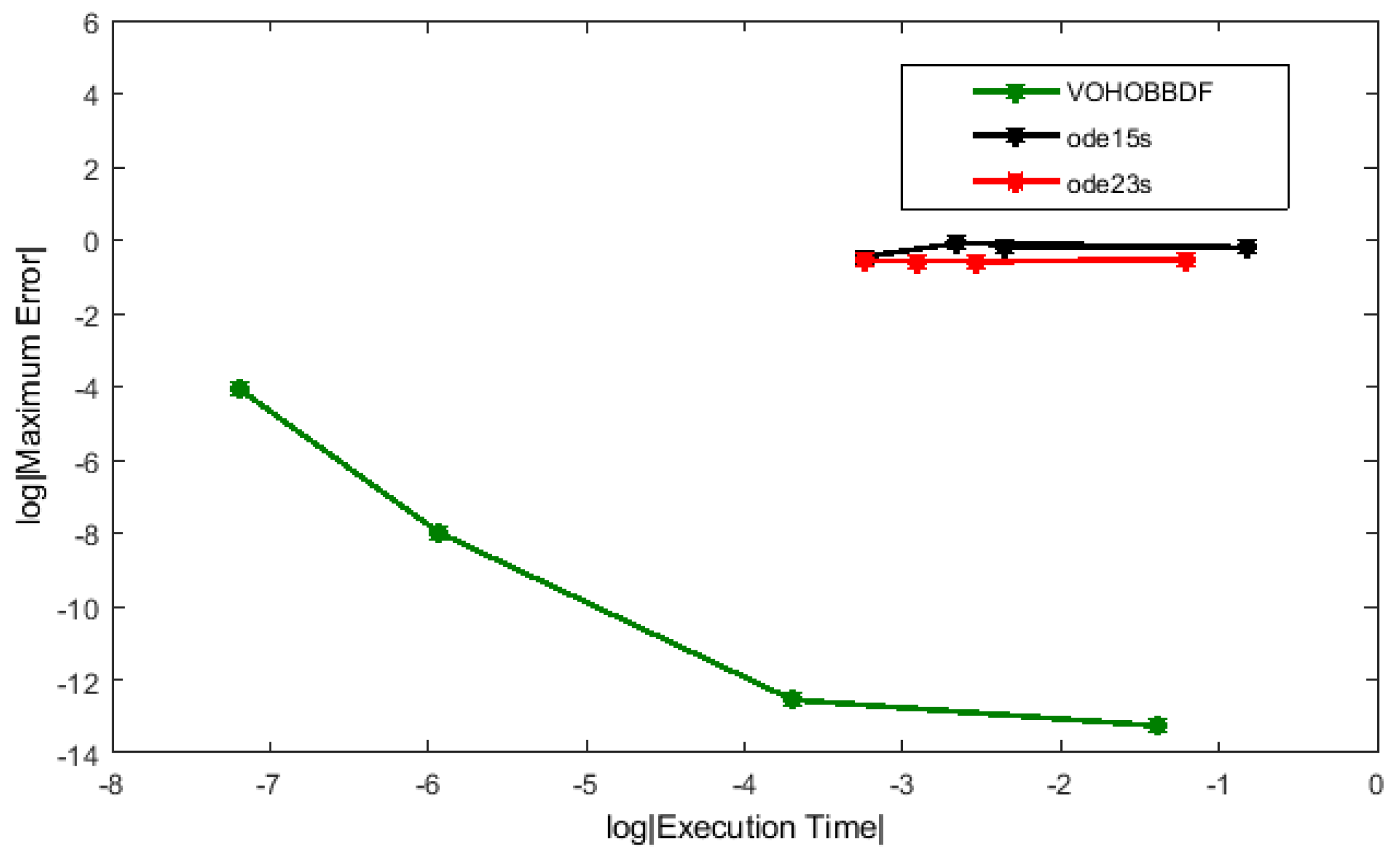
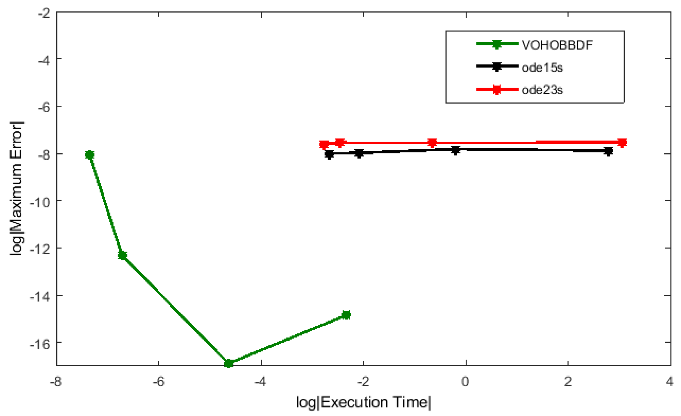
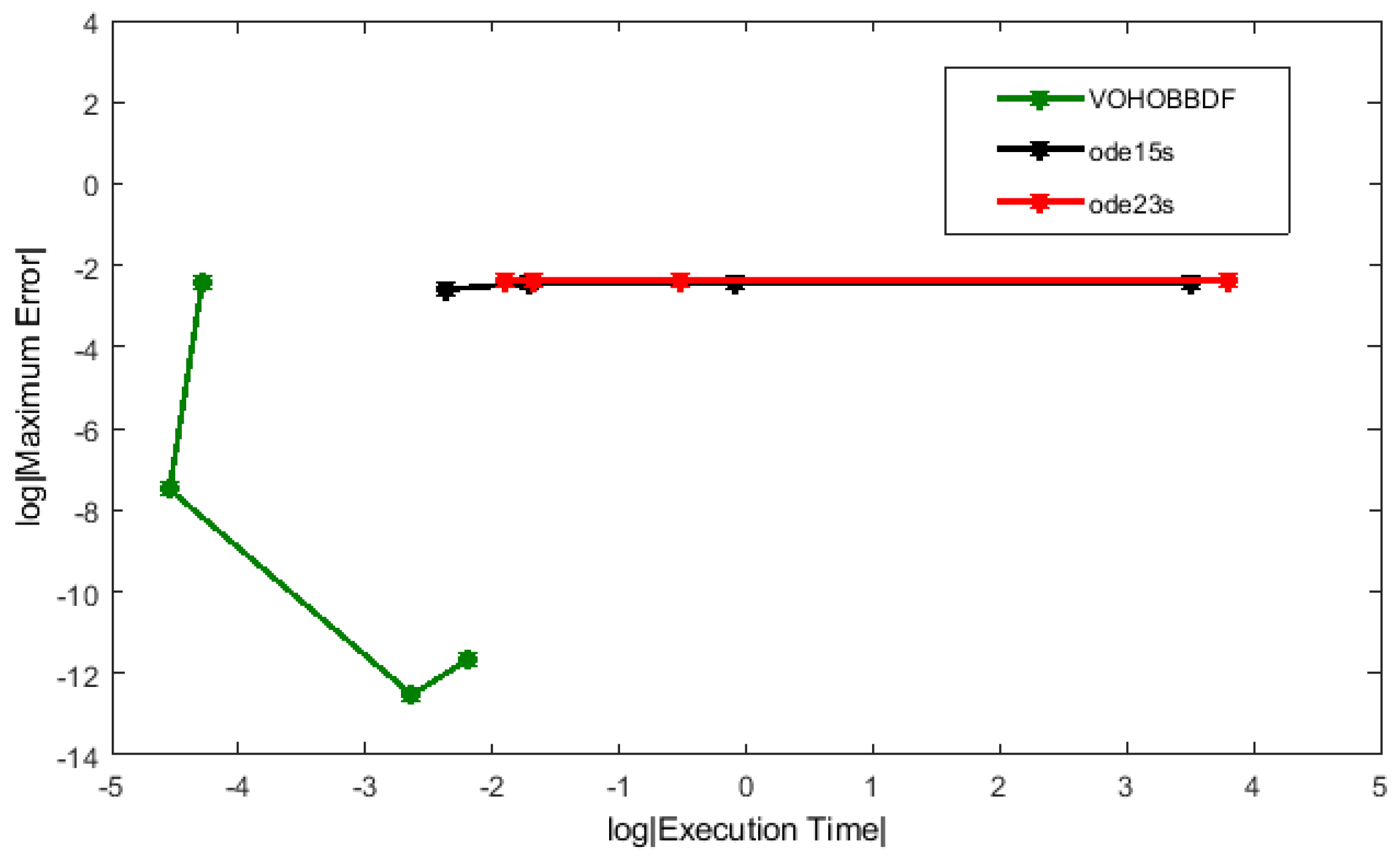
4. Numerical Experiments and Discussion

Three different problems were solved directly using the developed method by applying the variable order approach. To analyze the efficiency of applying this approach, the results were compared with two built-in stiff Matlab codes, ode15s and ode23s, which were designed to solve the stiff problems. However, to solve these problems using the Matlab codes, they need to be reduced into their equivalent systems of first order. The accuracy and efficiency of the methods are given in

Table 3. Numerical results for Problem 1.

h	Method	AE	ME	Total Steps	ET(s)
0.01	VOHOBBDF	9.52776 × ${10}^{-4}$	1.69964 × ${10}^{-2}$	100	0.000752
	ode15s	5.40856 $\times {10}^{-3}$	6.37651 $\times {10}^{-1}$	200	0.039062
	ode23s	1.02200 $\times {10}^{-2}$	5.75407 $\times {10}^{-1}$	200	0.039062
0.001	VOHOBBDF	2.13783 × ${10}^{-5}$	3.40432 × ${10}^{-4}$	1000	0.002652
	ode15s	7.73822 × ${10}^{-3}$	9.16663 × ${10}^{-1}$	2000	0.070312
	ode23s	9.62600 × ${10}^{-3}$	5.60735 × ${10}^{-1}$	2000	0.054687
0.0001	VOHOBBDF	2.21621 × ${10}^{-7}$	3.52619 × ${10}^{-6}$	10000	0.024842
	ode15s	7.75325 × ${10}^{-3}$	8.14285 × ${10}^{-1}$	20000	0.437500
	ode23s	9.96859 × ${10}^{-3}$	5.81096 × ${10}^{-1}$	20000	0.296875
0.00001	VOHOBBDF	1.32033 × ${10}^{-7}$	1.74158 × 10−6	100000	0.249087
	ode15s	7.74728 × ${10}^{-3}$	8.13635 × ${10}^{-1}$	200000	10.507812
	ode23s	9.57598 × ${10}^{-3}$	5.57189 × ${10}^{-1}$	200000	12.578125

,

Table 4. Numerical results for Problem 2.

h	Method	AE	ME	Total Steps	ET(s)
0.01	VOHOBBDF	5.76208 × ${10}^{-5}$	3.12829 × ${10}^{-4}$	100	0.000645
	ode15s	1.01716 × ${10}^{-5}$	3.34008 × ${10}^{-4}$	200	0.070312
	ode23s	2.31030 × ${10}^{-5}$	4.98225 × ${10}^{-4}$	200	0.062500
0.001	VOHOBBDF	8.29775 × ${10}^{-7}$	4.48794 × ${10}^{-6}$	1000	0.001214
	ode15s	1.01906 × ${10}^{-5}$	3.40308 × ${10}^{-4}$	2000	0.125000
	ode23s	2.31138 × ${10}^{-5}$	5.29203 × ${10}^{-4}$	2000	0.085937
0.0001	VOHOBBDF	8.47409 × ${10}^{-9}$	4.62483 × ${10}^{-8}$	10000	0.009719
	ode15s	7.21904 × ${10}^{-6}$	4.00145 × ${10}^{-4}$	20000	0.828125
	ode23s	2.30210 × ${10}^{-5}$	5.25468 × ${10}^{-4}$	20000	0.516075
0.00001	VOHOBBDF	9.96542 × ${10}^{-8}$	3.55634 × ${10}^{-7}$	100000	0.096912
	ode15s	7.52337 × ${10}^{-6}$	3.75244 × ${10}^{-4}$	200000	16.101562
	ode23s	2.31828 × ${10}^{-5}$	5.31723 × ${10}^{-4}$	200000	21.226562

and

Table 5. Numerical results for Problem 3.

h	Method	AE	ME	Total Steps	ET(s)
0.01	VOHOBBDF	4.50236 × ${10}^{-3}$	8.84316 × ${10}^{-2}$	100	0.013748
	ode15s	1.04430 × ${10}^{-1}$	1.32899 × ${10}^{+1}$	200	0.093750
	ode23s	1.57275 × ${10}^{-1}$	1.06758 × ${10}^{+1}$	200	0.187500
0.001	VOHOBBDF	3.15549 × ${10}^{-5}$	5.55627 × ${10}^{-4}$	1000	0.010650
	ode15s	8.07396 × ${10}^{-2}$	1.15260 × ${10}^{+1}$	2000	0.179687
	ode23s	1.55158 × ${10}^{-1}$	1.05471 × ${10}^{+1}$	2000	0.148437
0.0001	VOHOBBDF	2.07591 × ${10}^{-7}$	3.62885 × ${10}^{-6}$	10000	0.071776
	ode15s	7.30058 × ${10}^{-2}$	1.14937 × ${10}^{+1}$	20000	0.921875
	ode23s	1.57193 × ${10}^{-1}$	1.06936 × ${10}^{+1}$	20000	0.593750
0.00001	VOHOBBDF	5.32785 × ${10}^{-7}$	8.65595 × ${10}^{-6}$	100000	0.112163
	ode15s	7.28808 × ${10}^{-2}$	1.14840 × ${10}^{+1}$	200000	33.320312
	ode23s	1.54741 × ${10}^{-1}$	1.05336 × ${10}^{+1}$	200000	44.414062

for comparison purposes. Figure 1, Figure 2 and Figure 3 illustrate the results in Table 3, Table 4 and Table 5.

Let E be the error,

$${\left(E_i\right)}_n=\left|\frac{{\left(y_i\right)}_n-{\left(y\left(x_i\right)\right)}_n}{A+B{\left(y\left(x_i\right)\right)}_n}\right|$$

Therefore, the average error (AE) and maximum error (ME) are defined as

$$AE=\frac{{\displaystyle \sum _{i=1}^{TS}}{\displaystyle \sum _{i=1}^n}{\left(E_i\right)}_n}{n\left(TS\right)},$$

$$\mathit{ME}=\underset{1<i<TS}{max}\left(\underset{1<i<n}{max}{\left(E_i\right)}_n\right)$$

where TS is the total steps and n is the number of equations.

The general form for equivalent system of first order ODE is as follows.

$$\begin{array}{c}{y}_1^{\prime }=y_2,\\ y_2^{\prime }=y_3,\\ y_3^{\prime }=w{y}_1+v{y}_2+z{y}_3\end{array}$$

(9)

Refer to the general form of third order ODE in Equation (1) and its equivalent form of first order in Equation (4). The problems to be tested are as follows.

Problem 1

$\alpha =-\mathrm{27,000},\beta =-2700,\gamma =-90,$

Exact solution: $y\left(x\right)=e^{-30x}+4x{e}^{-30x}+9x^2{e}^{-30x},$

Initial conditions: $y\left(0\right)=1,y^{\prime }\left(0\right)=-26,y^{″}\left(0\right)=678,$

Interval: $[0,2]$

Equivalent system of first order

$w=-\mathrm{27,000},v=-2700,z=-90,$

Exact solutions:

$y_1=e^{-30x}+4x{e}^{-30x}+9x^2{e}^{-30x},$

$y_2=-26e^{-30x}-102x{e}^{-30x}-270x^2{e}^{-30x},$

$y_3=678e^{-30x}+2520x{e}^{-30x}+8100x^2{e}^{-30x}.$

Initial conditions:

$y_1\left(0\right)=1,$

$y_2\left(0\right)=-26,$

$y_3\left(0\right)=678.$

Problem 2

$\alpha =-1000,\beta =-300,\gamma =-30,$

Exact solution: $y\left(x\right)=-\frac{1}{2}{x}^2{e}^{-10x},$

Initial conditions: $y\left(0\right)=0,y^{\prime }\left(0\right)=0,y^{″}\left(0\right)=-1,$

Interval: $[0,2]$

Equivalent system of first order

$w=-1000,v=-300,z=-30,$

Exact solutions:

$y_1=-\frac{1}{2}{x}^2{e}^{-10x},$

$y_2=-e^{-10x}x+5x^2{e}^{-10x},$

$y_3=-e^{-10x}+20x{e}^{-10x}-50x^2{e}^{-10x}.$

Initial conditions:

$y_1\left(0\right)=0,$

$y_2\left(0\right)=0,$

$y_3\left(0\right)=-1.$

Problem 3

$\alpha =-\mathrm{15,000},\beta =-1850,\gamma =-75,$

Exact solution: $y\left(x\right)=3e^{-20x}+7e^{-25x}-13e^{-30x},$

Initial conditions: $y\left(0\right)=-3,y^{\prime }\left(0\right)=155,y^{″}\left(0\right)=-6125,$

Interval: $[0,2]$

Equivalent system of first order

$w=-\mathrm{60,000},v=-4700,z=-120,$

Exact solutions:

$y_1=3e^{-20x}+7e^{-25x}-13e^{-30x},$

$y_2=-60e^{-20x}-175e^{-25x}+390e^{-30x},$

$y_3=1200e^{-20x}+4375e^{-25x}-11700e^{-30x}.$

Initial conditions:

$y_1\left(0\right)=-3,$

$y_2\left(0\right)=155,$

$y_3\left(0\right)=-6125.$

5. Discussion

As evident from the results in Table 3, Table 4 and Table 5 and Figure 1, Figure 2 and Figure 3, the proposed method could improve the accuracy of all the test problems. The results also show that VOHOBBDF obtained the smallest maximum errors at different value of step sizes. Furthermore, the errors are also within the tolerance value. As shown in the results, VOHOBBDF successfully achieved less computational cost compared to both Matlab codes. It is clearly observed that the number of total steps was reduced to half and the method also sped up the execution time at all step sizes. Therefore, less time is needed to compute the solutions. This is due to the benefit of block method, where VOHOBBDF managed to produce two numerical approximations simultaneously at each step and approximate the solutions directly, thus decreasing the computational time.

6. Conclusions

This research demonstrates that the adaptive order approach applied to VOHOBBDF methods is significantly advantageous as it yields better performances over the built-in stiff Matlab codes. The approximate results of all the problems are better in accuracy as the results obtained lower maximum errors than both Matlab codes. The method also reduces computation time since the higher order problems can be solved directly. Hence, VOHOBBDF has proven its superior performances and reliability to be served as a direct solver for higher order stiff ODEs.

References

1. Suleiman, M.B.; Ibrahim, Z.B.; Rasedee, A.F.N.B. Solution of higher-order ODEs using backward difference method. Math. Probl. Eng. 2011, 2011, 810324. [Google Scholar] [CrossRef]
2. Yap, L.K.; Ismail, F. Four point block hybrid collocation method for direct solution of third order ordinary differential equations. In Proceedings of the 25th National Symposium on Mathematical Sciences, Kuantan, Malaysia, 27–29 August 2017; AIP Publishing: Melville, NY, USA, 2018; pp. 1–9. [Google Scholar]
3. Gear, C.W. The numerical integration of ordinary differential equations. In Mathematics of Computation; American Mathematical Society: Providence, RI, USA, 1967; pp. 21, 146–156. [Google Scholar]
4. Hijazi, M.; Abdelrahim, R. The Numerical Computation of three step hybrid block method for directly solving third order ordinary differential equations. Glob. J. Pure Appl. Math. 2017, 13, 89–103. [Google Scholar]
5. Adeyeye, O.; Omar, Z. New linear block method for third order ordinary differential Equations. J. Eng. Appl. Sci. 2018, 13, 4913. [Google Scholar]
6. Hussain, K.A.; Ismail, F.; Senu, N.; Rabiei, F. Fourth-order improved Runge–Kutta method for directly solving special third-order ordinary differential equations. Iran. J. Sci. Technol. 2017, 41, 429–437. [Google Scholar] [CrossRef]
7. Gear, C.W. The automatic integration of stiff ordinary differential equations. In Proceedings of IFIP Congress; North Holand Publishing Company: Amsterdam, The Netherlands, 1969; pp. 187–193. [Google Scholar]
8. Sumithra, B. Numerical solution of stiff system by backward euler method. Appl. Math. Sci. 2015, 9, 3303–3311. [Google Scholar] [CrossRef]
9. Abdi, A. Construction of high-order quadratically stable second-derivative general linear methods for the numerical integration of stiff ODEs. J. Comput. Appl. Math. 2016, 303, 218–228. [Google Scholar] [CrossRef]
10. Chollom, J.P.; Kumleng, G.M.; Longwap, S. High order block implicit multi-step (HOBIM) methods for the solution of stiff ordinary differential equations. Int. J. Pure Appl. Math. 2014, 96, 483–505. [Google Scholar] [CrossRef]
11. Ponalagusamy, R.; Ponnammal, K. A parallel fourth order rosenbrock method: Construction, analysis and numerical comparison. Int. J. Appl. Comput. Math. 2015, 1, 45–68. [Google Scholar] [CrossRef]
12. Suleiman, M.B.; Musa, H.; Ismail, F.; Senu, N. A new variable step size block backward differentiation formula for solving stiff IVPs. Int. J. Comput. Math. 2013, 90, 2391–2408. [Google Scholar] [CrossRef]
13. Zainuddin, N.; Ibrahim, Z.B.; Othman, K.I.; Suleiman, M.B. Direct fifth order block backward differentation formulas for solving second order ordinary differential equations. Chiang Mai J. Sci. 2016, 43, 1171–1181. [Google Scholar]
14. Ibrahim, Z.B.; Mohd Nasir, N.A.A.; Othman, K.I.; Zainuddin, N. Adaptive order of block backward differentiation formulas for stiff ODEs. Numer. Algebr. Control Optim. 2017, 7, 95–106. [Google Scholar] [CrossRef]
15. Asnor, A.I.; Yatim, S.A.M.; Ibrahim, Z.B. Algorithm of modified variable step block backward differentiation formulae for solving first order stiff ODEs. In Proceedings of the 25th National Symposium on Mathematical Sciences, Kuantan, Malaysia, 27–29 August 2017; AIP Publishing: Melville, NY, USA, 2018; pp. 1–11. [Google Scholar]
16. Ibrahim, Z.B.; Noor, N.M.; Othman, K.I. Fixed coefficient a(α) stable block backward differentiation formulas for stiff ordinary differential equations. Symmetry 2019, 11, 846. [Google Scholar] [CrossRef]
Figure 1. Efficiency graph for Problem 1.
Symmetry 11 01289 g001
Figure 2. Efficiency graph for Problem 2.
Symmetry 11 01289 g002
Figure 3. Efficiency graph for Problem 3.
Symmetry 11 01289 g003