An Improved Pigeon-Inspired Optimisation Algorithm and Its Application in Parameter Inversion

Abstract

Pre-stack amplitude variation with offset (AVO) elastic parameter inversion is a nonlinear, multi-solution optimisation problem. The techniques that combine intelligent optimisation algorithms and AVO inversion provide an effective identification method for oil and gas exploration. However, these techniques also have shortcomings in solving nonlinear geophysical inversion problems. The evolutionary optimisation algorithms have recognised disadvantages, such as the tendency of convergence to a local optimum resulting in poor local optimisation performance when dealing with multimodal search problems, decreasing diversity and leading to the prematurity of the population as the number of evolutionary iterations increases. The pre-stack AVO elastic parameter inversion is nonlinear with slow convergence, while the pigeon-inspired optimisation (PIO) algorithm has the advantage of fast convergence and better optimisation characteristics. In this study, based on the characteristics of the pre-stack AVO elastic parameter inversion problem, an improved PIO algorithm (IPIO) is proposed by introducing the particle swarm optimisation (PSO) algorithm, an inverse factor, and a Gaussian factor into the PIO algorithm. The experimental comparisons indicate that the proposed IPIO algorithm can achieve better inversion results.

1. Introduction

First proposed in the early 1990s, the swarm intelligence algorithm is a stochastic optimisation algorithm that is largely inspired by the phenomena of biological swarm intelligence in nature and mimics the behaviour of social animals [1]. Swarm intelligence means that a swarm constituted by a large number of simple individuals without intelligence shows intelligent behaviour through the simple cooperation of the individuals with each other. Under the guidance of appropriate evolutionary mechanisms, swarm intelligence takes an explicit form through the interaction among individuals. The swarm intelligence algorithm simulates the search and optimisation process of the individuals’ evolution or foraging process. In these algorithms, the individuals in nature are represented by the points in the search space. The objective function of the problem at issue is measured as the individuals’ ability to adapt to the environment, while the individuals’ survival of the fittest process or foraging process is analogous to the iterative process. In the process, a poor feasible solution is replaced by a good feasible solution, which gives rise to an iterative search algorithm characterised with the “generation + test” feature and represents a self-adaptive artificial intelligence technique for solving the extremum problems [2]. Based on swarm intelligence research, a variety of swarm intelligence optimisation algorithms have been proposed.

In 1991, Dorigo et al. [3] proposed the ant colony optimisation (ACO) algorithm by simulating the foraging behaviour of ant colonies in nature. The ACO algorithm enables the reorganisation of its own database according to changes in the environment to achieve the evolution of the algorithm’s solving ability. However, the ACO algorithm requires a long search time, convergences slowly, and is easily trapped in local optima.

In 1995, Kennedy and Eberhart [4] proposed the particle swarm optimisation (PSO) algorithm through the study of swarm phenomena in nature. The PSO algorithm manifests strong robustness and fast convergence when processing complex multimodal optimisation problems, but it still has the inherent shortcomings of traditional bionic intelligent algorithms and is easily trapped in local optima.

Delice et al. [5] proposed a new PSO algorithm with negative knowledge to address the mixed-model two-sided assembly line balancing problem, showing an enhanced solving ability. Chatterjee [6] proposed a PSO-based approach to train the neural network (NN-PSO) to address the issues of local optimum trapping and premature convergence, common to traditional learning methods. The NN-PSO can solve the failure problem of multi-story reinforced concrete structures by detecting the failure probability of the structures. This detection is of great significance in the prevention of enormous losses due to structural failure.

In long-range homing, pigeons need the help of both the geomagnetic field and the landform, using the former to determine the general direction and the latter to amend the actual direction, thereby achieving the purpose of accurately locking the position. Inspired by the homing behaviour of pigeons in nature, in 2014, Duan et al. [7] proposed the pigeon-inspired optimisation (PIO) algorithm, a pigeon homing behaviour-based swarm intelligence optimisation algorithm that has made remarkable achievements in recent years in various fields, such as unmanned aerial vehicle (UAV) formation, parameter change control, and image processing.

Duan et al. [8] proposed a cooperative control method for UAV tight formation based on the optimisation of the predatory escape behaviour of pigeons. Following the basic idea of PIO, the structure is adjusted, and the predatory escape mechanism is introduced to improve the overall performance and to address the issue of easily trapping the PIO in local optima. The three-dimensional route planning for unmanned combat aerial vehicles (UCAVs) is a complex optimisation problem that focuses on the routing optimisation of aircraft with different constraints in complex, dynamic environments [9]. To address this problem, Zhang and Duan proposed a new predator-prey PIO (PPPIO) algorithm, which improves the global optimisation performance and convergence rate by adopting the concept of predator and prey. Dou et al. [10] proposed a new method to obtain the optimal parameters for the carrier-based aircraft controller, wherein the PIO is used in the optimisation of the prediction control parameters of the model to quickly obtain the global optimal solution while enabling easier and more effective choice of parameters through the PIO algorithm. Duan et al. [11] used the PIO to optimise the parameters of the echo state neural network to restore blurred and noisy images. In addition, the PIO improved using the orthogonal strategy which exhibits higher adaptability in performance than the existing bionic optimisation algorithms. Saranya et al. [12] proposed a PIO-based method to obtain the optimal threshold for automatic detection and extraction of the features of follicular cysts from ovary images. They demonstrated through contrast experiments that the proposed method can find better solutions with faster convergence rates. Lei et al. [13] successfully applied the PIO method to protein complex detection, which is key to understanding the principles of cellular organisation. By optimising the parameters of ε and MinPts in density-based spatial clustering of applications with noise (DBSCAN) using PIO, Lei et al. developed a new method, the pigeon-inspired optimisation DBSCAN (P_DBSCAN) to detect protein complexes in the dynamic protein-protein interaction network. In recent years, the PIO algorithms have been extensively applied.

The main contributions of this paper are as follows:

• An improved PIO algorithm (IPIO) is proposed by introducing the particle swarm optimisation (PSO) algorithm, an inverse factor, and a Gaussian factor into the PIO algorithm. In order to verify the effectiveness of the improvement, the benchmark functions are used to do the experiments and compare the experimental results with other algorithms.
• The improved algorithm for the pre-stack AVO elastic parameter inversion is used. The experimental comparison results with other optimisation algorithms indicate that the proposed IPIO algorithm can achieve better inversion results.

2. PIO Algorithm

2.1. PIO Algorithm and Its Improvement

The main factors affecting the pigeons’ homing behaviour are the sun, the Earth’s magnetic field, and landmarks. The pigeons use different navigation tools at different stages of the journey. Studies on the pigeons’ navigation behaviour have revealed that in the initial stage of homing, the pigeons use the compass-like navigational tool most of the time. In the middle part of the journey, they switch to the landmark navigation tool and, at the same time, re-evaluate their route and make necessary corrections.

According to the pigeons’ homing behaviour and by imitating the mechanism that pigeons use different navigation tools at different stages, two different operator models are proposed for the PIO algorithm [7] as follows:

(1) The map and compass operator. The pigeons perceive the Earth’s magnetic field via magnetic objects and then form a map in their mind. They use the height of the sun as a compass to adjust their flight direction, and as they approach the destination, their dependence on the sun and magnetic objects is reduced.

Similar to the PSO algorithm, in the PIO algorithm, pigeons have their own position and velocity information, with the following updated Formulas (1) and (2) for each pigeon.

$$V_i^{N_c}=V_i^{N_c-1}{e}^{-R\times N_c}+rand(X_{gbest}-X_i^{N_c-1})$$

(1)

$$X_i^{N_c}=X_i^{N_c-1}+V_i^{N_c}$$

(2)

where R is the map and compass factor, with a range of 0 to 1; rand is a random number in the range of 0 to 1; Nc is the current number of iterations; and X_gbest is the global optimal position obtained by comparing the positions of all the pigeons after Nc-1 iteration cycles. Once the required number of iterations is reached, the operation of the map and compass operator is stopped and the landmark operator is activated.

(2) The landmark operator. The landmark operator is used to simulate the influence of landmarks on the pigeons’ navigation. When pigeons fly near the destination, they rely more on nearby landmarks. If they are familiar with the landmarks, they fly directly to the destination. Otherwise, they follow the pigeons that are familiar with the landmarks. In each iteration, the number of pigeons is halved by discarding the pigeons that are far from the destination since they are unfamiliar with the landmarks and no longer have the ability to distinguish the route. The central position of the remaining pigeons is X_center, which is used as a landmark, i.e., as a reference flight direction. Accordingly, the position of the ith pigeon (X_i) is updated using the Formulas (3)–(5).

$$X_{center}^{N_c-1}=\frac{{\displaystyle \sum _{i=1}^{N^{{}^{N_c-1}}}{X}_i^{N_c-1}F(X_i^{N_c-1})}}{N^{{}^{N_c-1}}{\displaystyle \sum _{i=1}^{N^{{}^{N_c-1}}}F(X_i^{N_c-1})}}$$

(3)

$$N^{N_c}=\frac{N^{{}^{N_c-1}}}{2}$$

(4)

$$X_i=X_i^{N_c-1}+rand(X_{center}^{N_c-1}-X_i^{N_c-1})$$

(5)

where, $F(X_i^{N_c-1})=\{\begin{array}{l}\frac{1}{fitness(X_i^{N_c-1})+\epsilon },Forminimisationproblems\\ fitness(X_i^{N_c-1}),Formaximisationproblems\end{array}$. Similarly, once the maximum number of iterations is reached, the operation of the landmark operator is stopped.

The PIO algorithm has a fast convergence rate but can be very easily trapped in local optima. Moreover, the population at every step shows an aggregation state, making it impossible to perform a large number of iterations. In general, after the iterations of the first operator, all the individuals are essentially overlapped, leading to the situation where the second operator has no chance to have a turn. To address the above shortcomings of the PIO algorithm, some modifications have been made.

(1) Hybrid particle swarm algorithm

In the map and compass operator of the PIO algorithm, all the individuals move towards the optimal or sub-optimal individual. When the initial position is not near the true global optimal solution, it can cause other individuals to search in the wrong space along the route, and ultimately, be unable to find the optimal solution. Moreover, the population exhibits an aggregation state at each step, decreasing the diversity.

The PIO algorithm is similar to the PSO algorithm in that both simulate the flight characteristics of living creatures, both use the position of the current optimal individual as a reference, and both have the advantages of fast convergence and simple implementation. The differences between the two are that in the PSO algorithm, individuals not only use the position of the current optimal individual as a reference, but also take their own optimal positions as references, using the updated Formulas (6) and (7).

$$V_i^{N_c}=\omega \ast V_i^{N_c-1}+c_1\ast rand\ast \left(X_{pbest}-X_i^{X_c-1}\right)+c_2\ast rand\ast \left(X_{gbest}-X_i^{X_c-1}\right)$$

(6)

$$X_i^{N_c}=X_i^{X_c-1}+V_i^{N_c}$$

(7)

Compared with the map and compass operator of the PIO algorithm, the speed update formula of the PSO algorithm introduces the individuals’ own optimal positions, which can avoid the aggregation state of all the particles, and thus increase the diversity of the swarm. Therefore, for the improved PIO algorithm (IPIO) proposed in this study, the original map and compass operator are replaced by the PSO algorithm.

(2) Reverse learning mechanism

After the operation of the map and compass operator, if all the individuals are basically overlapped, the landmark operator is likely to be invalid, causing the algorithm to be trapped in local optima, and thus seriously affecting its performance. To avoid such a situation, reverse learning is introduced to the algorithm and combined with particle learning of the particle swarm to effectively balance the global search and local mining capabilities.

The concept of reverse learning was proposed by Tizhoosh in 2005, who argued that the efficiency of the algorithm can be enhanced by simultaneously considering the current solution and its reverse solution in the search process, and then selecting the better one of the two [14]. In the proposed algorithm, the elitist selection strategy based on the current solution and the reverse solution is used to accelerate the convergence of the algorithm. To avoid local optima and improve algorithm performance, a reverse learning strategy is introduced to perform general reverse learning on the individuals’ position attributes and the next-generation population is selected through a comparison. In other words, based on the original population, a reverse population is generated, in which the individuals correspond pair-wisely to those in the original population. When making selections, the fitness value of each individual of the two populations is calculated, and if the reverse individual of an individual is superior to the individual itself in terms of the fitness value, the reverse individual is retained, and, otherwise, the original individual is retained. The next-generation population thus selected remains unchanged in size. The reverse solution is obtained using Formula (8).

$$X_i^{\prime }=a_i+b_i-X_i$$

(8)

where $a_i$ and $b_i$ are the upper and lower thresholds, respectively, of the solution. A comparison of the current solution with its reverse solution causes the solution to be more complete and avoids entrapment in local optima while ensuring that the second operator (i.e., the landmark operator) plays a better role.

(3) Gaussian factor.

The Gaussian factor has been introduced into the PIO algorithm [15], and it was noted that its use of random numbers with a uniform distribution results in, to some extent, a full search capability. A Gaussian distribution, also known as a normal distribution, has been widely used in natural and social sciences. It has two parameters, i.e., μ and σ². The parameter μ is the mean or expected value (which is also the mid-value and the mode) of the distribution and the parameter σ is the standard deviation (and its variance is σ²).

In many cases, the optimisation algorithm should have the ability to ensure that the destination is correct when carrying out a focused search. However, this requirement cannot be satisfied using a method for obtaining random numbers with a uniform distribution. The search equation in the landmark operator of the PIO satisfies the latent premise of a Gaussian distribution and can be improved to achieve global optima. Therefore, the Gaussian random numbers are introduced into the landmark operator to enhance their ability to search for the optima.

The position update formula of the improved landmark operator is as Formulas (9) and (10).

$$\{\begin{array}{ll}{X}_i\left(T\right)=X_i\left(T-1\right)+2\left(R_1-0.5\right)·\left(x_c\left(T\right)-X_i\left(T-1\right)\right)·mn& if(R_2>p)\\ X_i\left(T\right)=X_i\left(T-1\right)+2\left(R_1-0.5\right)·\left(x_c\left(T\right)-X_i\left(T-1\right)\right)·2n& if\left(R_2\le p\right)\end{array}$$

(9)

$$\{\begin{array}{l}m=\left|R_n\right|\\ n=0.5-0.25\frac{T}{T_2}\end{array}$$

(10)

where p is a flexible parameter that is used to balance a Gaussian distribution and a uniform distribution, R₁ and R₂ are two random numbers between 0 and 1, R_n is a Gaussian random number between 0 and 1, and T₂ is the maximum number of iterations.

From what has been discussed above, the steps of the proposed IPIO algorithm are as follows and the flow chart of the improved algorithm is shown in Figure 1.

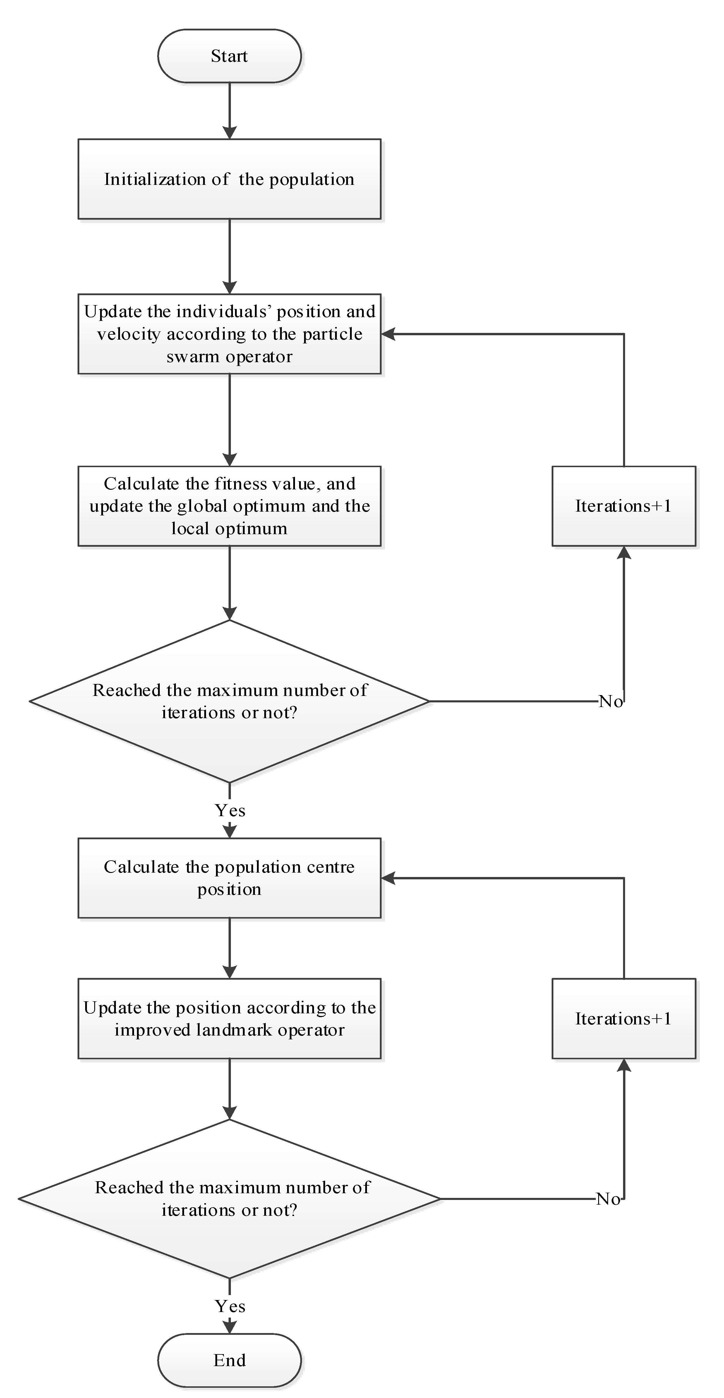
• Initialise the parameters, initialise the population, calculate the fitness value of each individual in the population, and select the optimal position $X_{gbest}$ of the population.
• Update the position and speed of each individual according to the PSO algorithm, and calculate the position of the individual’s corresponding reverse individual.
• Calculate the fitness value, compare the fitness values of the individual and its reverse individual, retain the better one of the two, remove the poor one, and update the global optimum and the historical optimum of each individual.
• Determine whether the maximum number of iterations of the particle swarm operator is reached. If yes, proceed to the next step, otherwise return to Step 2.
• Calculate the centre position of the population using the landmark operator of the PIO algorithm.
• Update the position of each individual based on the improved landmark operator.
• Calculate the fitness value, and update the global optimum.
• Determine whether the maximum number of iterations of the landmark operator is reached. If yes, terminate the operation, otherwise return to Step 6 to operate until the iteration is stopped.

2.2. Experimental Results and Analysis

To verify the effectiveness of the proposed IPIO algorithm and compare it with the basic genetic algorithm (GA), the differential evolution (DE) algorithm, the PSO algorithm, and the PIO algorithm, tests were performed using a variety of single-modal and multi-modal test functions, as shown in Formulas (11)–(19).

$$\begin{array}{l}{f}_1(x)={\displaystyle \sum _{i=1}^D{t}_i}+200D\\ t_i=\{\begin{array}{cc}-160+y_i^2\hfill & if(y_i<0)\\ \frac{160}{15}(y_i-15)\hfill & if(0\le y_i\le 15)\\ \frac{200}{5}(15-y_i)\hfill & if(15\le y_i\le 20)\\ -200+{(y_i-20)}^2\hfill & if(y_i>20)\end{array}\\ y=x+20\end{array}$$

(11)

$$\begin{array}{l}{f}_2(x)={\displaystyle \sum _{i=1}^D{t}_i}+D\\ t_i=\{\begin{array}{cc}{y}_i^2& if(y_i<0or{y}_i>1)\\ -\exp [-2\log (2)\cdot {\left(\frac{y_i-0.1}{0.8}\right)}^2]\cdot {\sin }^6(5\pi {\mathrm{y}}_i)& if(0\le y_i\le 1)\end{array}\\ i=1,2,\dots ,D\\ y=x+0.1\end{array}$$

(12)

$$f_3(x)={\displaystyle \sum _{i=1}^D[x_i^2-10\cos (2\pi x_i)+10]}$$

(13)

$$f_4(x)=x_1^2+{10}^6{\displaystyle \sum _{i=2}^D{x}_i^2}$$

(14)

$$f_5(x)={\displaystyle \sum _{i=1}^{n-1}[{(x_i^2)}^{x_{i+1}^2+1}+{(x_{i+1}^2)}^{x_i^2+1}]}\hspace{1em}{x}_i\in [-1,4]$$

(15)

$$f_6(x)={\displaystyle \sum _{i=1}^n[{(x_i-1)}^2+{(x_1-x_i^2)}^2]}\hspace{1em}x\in [0,10]$$

(16)

$$\begin{array}{l}{f}_7(x)={\displaystyle \sum _{i=1}^D{t}_i}+200D\\ t_{\mathrm{i}}=\{\begin{array}{cc}-200+x_i^2\hfill & if(x_i<0)\\ -80(2.5-x_i)\hfill & if(0\le x_i<2.5)\\ -64(x_i-2.5)\hfill & if(2.5\le x_i<5)\\ -64(7.5-x_i)\hfill & if(5\le x_i<7.5)\\ -28(x_i-7.5)\hfill & if(7.5\le x_i<12.5)\\ -28(17.5-x_i)\hfill & if(12.5\le x_i<17.5)\\ -32(x_i-17.5)\hfill & if(17.5\le x_i<22.5)\\ -32(27.5-x_i)\hfill & if(22.5\le x_i<27.5)\\ -80(x_i-27.5)\hfill & if(27.5\le x_i\le 30)\\ -200+{(x_i-30)}^2\hfill & if(x_i>30)\end{array}\end{array}$$

(17)

$$\begin{array}{l}{f}_8(x)={\displaystyle \sum _{i=1}^D{t}_i}+D\\ t_i=\{\begin{array}{ll}\begin{array}{cc}{y}_i^2& if(y_i<0or{y}_i>1)\\ -{\sin }^6(5\pi y_i)& if(0\le y_i\le 1)\end{array}& i=1,2,\dots ,D\end{array}\\ y=x+0.1\end{array}$$

(18)

$$\begin{array}{l}{f}_9(x)={\displaystyle \sum _{i=1,3,5,\dots }^{D-1}[{(y_i^2+y_{i+1}-11)}^2+{(y_i+y_{i+1}^2-7)}^2]}\\ y_i=\{\begin{array}{ll}\begin{array}{ll}{x}_i+3& if i is odd number\\ x_i+2& if i is even number\end{array}& i=1,2,\dots ,D\end{array}\\ D must be an even number\end{array}$$

(19)

The independent variable range, dimension, optimal value, and solution category of each test function are shown in

Table 1. Test function information.

Function	Range of Independent Variable	Dimension	Optimal Value	Category
f(1)	[−100,100]	5	0	Single solution
f(2)	[−100,100]	5	0	Single solution
f(3)	[−100,100]	6	0	Single solution
f(4)	[−100,100]	5	0	Single solution
f(5)	[−1,4]	5	0	Single solution
f(6)	[0,10]	5	0	Single solution
f(7)	[−100,100]	5	0	Multiple solutions
f(8)	[−100,100]	5	0	Multiple solutions
f(9)	[−100,100]	6	0	Multiple solutions

.

The experimental results of the test functions are shown in

Table 2. Experimental results.

Function	Algorithm	Minimum Value	Maximum Value	Mean
f(1)	GA	2.56 × 10−3	5.14 × 10−1	1.01 × 10−1
	DE	3.94 × 10−2	45.08599	27.59336
	PSO	3.60 × 10−1	4.224161	1.934762
	PIO	1.32 × 10−7	3.55 × 10−2	8.44 × 10−3
	IPIO	5.69 × 10−8	3.71 × 10−5	5.42 × 10−6
f(2)	GA	1.19 × 10−1	1.604513	5.17 × 10−1
	DE	4.63 × 10−7	11.1002	1.684983
	PSO	2.213867	4.607223	3.56288
	PIO	8.84 × 10−5	3.376968	1.703053
	IPIO	3.82 × 10−14	2.15 × 10−1	1.69 × 10−2
f(3)	GA	5.81 × 10−2	2.706744	1.060794
	DE	2.44 × 10−8	55.00046	7.248065
	PSO	7.609825	20.19414	15.15247
	PIO	8.81 × 10−9	8.328467	1.403083
	IPIO	1.07 × 10−14	1.15 × 10−1	5.73 × 10−3
f(4)	GA	1.90 × 10−2	4659.428	594.2779
	DE	9.68 × 10−2	22078.02	3841.383
	PSO	11827.93	3459811	362612.9
	PIO	5.26E + 02	114849.4	23962.32
	IPIO	3.88 × 10−8	318704.3	1.63E+04
f(5)	GA	1.67 × 10−11	9.68 × 10−6	1.81 × 10−6
	DE	2.29 × 10−6	4.11 × 10−1	3.09 × 10−2
	PSO	1.21 × 10−4	8.53 × 10−4	4.84 × 10−4
	PIO	1.62 × 10−7	2.32 × 10−3	3.23 × 10−4
	IPIO	3.87 × 10−24	5.45 × 10−19	7.82 × 10−20
f(6)	GA	6.56 × 10−4	7.93 × 10−3	3.40 × 10−3
	DE	3.35 × 10−6	30.11047	7.679355
	PSO	4.68 × 10−4	1.67966	8.87 × 10−2
	PIO	4.02 × 10−1	3.06216	1.59
	IPIO	9.86 × 10−32	6.99 × 10−15	6.79 × 10−16
f(7)	GA	2.99 × 10−3	2.68 × 10−2	1.09 × 10−2
	DE	7.31 × 10−2	5.163348	1.671903
	PSO	3.07 × 10−1	4.484861	1.868947
	PIO	0.00	86.51133	33.82977
	IPIO	7.45 × 10−9	6.22 × 10−5	4.70 × 10−6
f(8)	GA	2.82 × 10−4	2.18 × 10−1	3.22 × 10−2
	DE	8.06 × 10−6	8.353849	9.78 × 10−1
	PSO	1.772018	3.991754	3.012487
	PIO	3.02 × 10−5	3.41 × 10−2	1.66 × 10−4
	IPIO	3.55 × 10−15	3.73 × 10−3	2.26 × 10−4
f(9)	GA	3.30 × 10−4	1.908191	4.45 × 10−1
	DE	4.88 × 10−3	295.5104	21.82682
	PSO	9.761999	47.82482	24.92847
	PIO	3.06 × 10−4	2.236064	1.41 × 10−1
	IPIO	5.50 × 10−12	0.058537	2.93 × 10−3

.

The above experimental comparison indicates that for test Functions 1, 3, 5, 6 and 7, the IPIO algorithm significantly outperforms other methods (GA, DE, PSO, and PIO), and specifically, the results for test Functions 5 and 6 using the IPIO algorithm are very near to the optimal values. For test Functions 2, 8, and 9, the IPIO algorithm showed a slightly higher performance than the GA, while the DE, the PSO, and the PIO algorithms performed poorly. For test Function 4, all algorithms performed poorly during optimisation. In summary, the measurements of nine multimodal functions indicate that the proposed IPIO algorithm has a high optimisation ability and can be used to solve the pre-stack amplitude variation with offset (AVO) elastic parameter inversion problem.

3. Pre-stack AVO Elastic Parameter Inversion Problem

In seismic exploration, seismic information is used for oil exploration. This information may reflect the trend of change in reservoir parameters. Therefore, it is also used to predict reservoir parameters. Pre-stack seismic data contain more fluid information than post-stack seismic data, and the pre-stack inversion method presents significant advantages, such as a stable result, high resolution, and strong controllability. The AVO technique uses the elastic wave theory as the basis to study and analyse the characteristics of the variation of the seismic reflection amplitude with offset using the pre-stack common depth point to understand the relation between the reflection coefficient and the incident angle. This is then used to analyse the lithological characteristics and physical parameters above and below the reflection interface, and further predict and judge the fluid properties and lithology of the reservoir [16,17,18,19]. Pre-stack seismic data contains numerous useful information that can be used to predict underground oil and gas conditions, of which three elastic parameters, i.e., P-wave velocity $V_p$, S-wave velocity $V_s$, and density $\rho$, are key parameters that indirectly reflect the saturation state of underground oil and gas [20,21,22,23,24,25]. By using the AVO information to solve the approximate formula of the Zoeppritz equation, the pre-stack inversion obtains the elastic parameters that reflect the characteristics of underground rock directly, i.e., P-wave velocity, S-wave velocity and density. The inversion of pre-stack AVO elastic parameters requires the construction and then the optimisation of a suitable objective function, which is generally nonlinear. In theory, multiplicity is present in inversion. In the inversion process, multiple sets of solutions that can fit the observation data to the same extent can be obtained. However, it is difficult to confirm which set of solutions is closer to the real model. Therefore, the inversion problem exhibits multiplicity and non-uniqueness. Relative to linear inversion methods, intelligent optimisation algorithms do not depend on the initial model and are easy to implement. Therefore, they are suitable for the inversion of multi-parameter and multi-extremum geophysical problems. In the mid-1980s, nonlinear global intelligent optimisation inversion techniques began to receive the attention of researchers in the geophysical field. New ideas and methods in other areas have been continuously introduced since that time and have many successful applications [22,23,24,25,26,27,28,29,30,31,32,33,34,35,36].

The basic steps for solving the pre-stack AVO elastic parameter inversion problem are as follows. First, the three parameters are obtained through a series of operations, next the reflection coefficient is calculated by substituting the three parameters into the approximate equation, then the seismic data are obtained by convolving the reflection coefficient and the seismic wavelet, and finally, the obtained seismic data are compared with the actual seismic data to determine the inversion accuracy, i.e., when the two sets of data are close and the three calculated parameters are similar to the three actual parameters, the inversion accuracy is considered high. Since the three calculated parameters are within the range calculated based on well-logging data, and three smooth curves can be generated by connecting the data of all the layers corresponding to the three parameters, the pre-stack AVO elastic parameter inversion can also be viewed as a global numerical optimisation problem with continuous variables.

3.1. Inversion Model

One of the main steps in solving the pre-stack AVO elastic parameter inversion problem is to establish the inversion convolution model. The main steps of establishing the convolution model are as following: First, calculate the reflection coefficient $R_{\mathrm{pp}}$. In this study, the approximation formula of Aki and Richard [37] is used to calculate $R_{\mathrm{pp}}$ as Formula (20).

$$R_{\mathrm{pp}}(\theta )=\frac{1}{2}(1+{\tan }^2\theta )\frac{\Delta V_p}{\overline{V_p}}-(4{\gamma }^2{\sin }^2\theta )\frac{\Delta V_s}{\overline{V_s}}+\frac{1}{2}(1-4{\gamma }^2{\sin }^2\theta )\frac{\Delta \rho }{\overline{\rho }}$$

(20)

where $\Delta V_p$, $\Delta V_s$ and $\Delta \rho$ are the differences of $V_p$, $V_s$ and $\rho$, respectively, between the upper and lower layers; $\overline{V_p}$, $\overline{V_s}$ and $\overline{\rho }$ are the mean values of $V_p$, $V_s$ and $\rho$, respectively, of the upper and lower layers; $\theta$ is the angle; and $\gamma =\frac{V_s}{V_p}$, which is calculated based on the actual measurements. Therefore, the $R_{\mathrm{pp}}$ calculated using this formula can be used as a component of the seismic record convolution operation.

Second, obtain the seismic wavelet. The seismic wavelet is another component of the seismic record convolution model. Seismic record data can be obtained by convolving the seismic wavelet and the reflection coefficient, which is suitable for establishing the forward model and synthesising seismic data gathers. In this study, the Ricker wavelet, a zero-phase seismic wavelet, is adopted, using Formula (21).

$$f(t)=(1-2{\pi }^2{V}_m{}^2{t}^2)e^{-{\pi }^2{V}_m{}^2{t}^2}$$

(21)

where $V_m$ is the main frequency, and t is the time, which can be set manually.

Third, perform the convolution operation on the Ricker wavelet and the reflection coefficient, using Formula (22).

$$s(\theta )=R_{\mathrm{pp}}(\theta )\ast f(t)+n(t)$$

(22)

where $R_{\mathrm{pp}}(\theta )$ is the reflection coefficient function, $f(t)$ is the seismic wavelet, and $n(t)$ is the noise, which is neglected in this study. The calculated $s(\theta )$ is used to construct the objective function.

3.2. Inversion Results Evaluation

The simulation-optimisation method converts the pre-stack AVO elastic parameter inversion problem to an optimisation problem, which is then solved using the optimisation algorithm. From the perspective of optimisation, when the difference between the inversion seismic data generated by the optimised elastic parameter and the actual seismic record data is 0 or less than a specified threshold, the elastic parameter is considered satisfactory. As the optimisation algorithm judges the performance of each individual based on the fitness function converted from the objective function, the performance of the objective function constructed specifically for the inversion problem is the main factor affecting the effectiveness of the pre-stack AVO elastic parameter inversion. In this study, the approximation equation of Aki and Richard is first used to obtain $R_{pp}$, i.e., the reflection coefficient of the p-wave, then the synthetic seismic record data is obtained by convolving $R_{pp}$ and the wavelet. Assume the number of sampling points is n, and for each point, m different angles are required, giving rise to $n\times m$ entries of seismic record data. Lastly, the sum of squares of the differences between the m sets of seismic record data obtained through the optimisation and the actual record data of each sampling point is calculated, which is then divided by m, and the sum of squares of difference data of n sampling points is then divided by n. Taking the square root of the final result yields the solution. Based on the above formulas, the inversion objective function is Formula (23).

$$f(x)=\sqrt{\frac{{\displaystyle \sum _{i=1}^n{\displaystyle \sum _{j=1}^m(s({\theta }_{i,j})}}-s^{\prime }({\theta }_{i,j}){)}^2}{n\times m}}$$

(23)

where $s({\theta }_{i,j})$ is the forward seismic record and $s^{\prime }({\theta }_{i,j})$ is the inverse seismic record.

Since the reflection coefficient $R_{\mathrm{pp}}$ is calculated through the elastic parameters $V_p$, $V_s$ and $\rho$, and the same set of inverse seismic record data obtained through the calculation are generated from infinite combinations of $V_p$, $V_s$ and $\rho$, there are cases in which the inverse seismic record data are calculated with all three parameters having errors identical to those calculated with one parameter having errors and two parameters not having errors. To better evaluate the performance of the optimisation algorithm in the pre-stack AVO elastic parameter inversion, the Pearson product-moment correlation coefficient (PPMCC or PCCs) is adopted to measure the correlation between the inversed three parameters and the actual three parameters. The higher the absolute value of the correlation coefficient is, the stronger the correlation; the closer the correlation coefficient is to 1 or −1, the stronger the correlation; and the closer the correlation coefficient is to 0, the weaker the correlation. The correlation coefficient function is Formula (24).

$$r=\frac{{\displaystyle \sum _{i=1}^n\left(X_i-\overline{X}\right)\left(Y_i-\overline{Y}\right)}}{\sqrt{{\displaystyle \sum _{i=1}^n{\left(X_i-\overline{X}\right)}^2}}•\sqrt{{\displaystyle \sum _{i=1}^n{\left(Y_i-\overline{Y}\right)}^2}}}$$

(24)

where $X_i$ is the standard value of a certain parameter of the three parameters, and $Y_i$ is the corresponding inversion value, and $\overline{X}$, $\overline{Y}$ are the means of a set of values.

From the complexity of the solution process of seismic data, a small objective function does not necessarily mean a high correlation coefficient of the three parameters, and vice versa. However, when the objective function value reaches its theoretical optimal value of 0, the correlation coefficients of $V_p$, $V_s$ and $\rho$ also reach their theoretical optimal value of 1. Therefore, in this study, the objective function and the correlation coefficient are combined to evaluate the performance of the inversion. The ultimate goal is to have a small objective function through the inversion and simultaneously, the correlation coefficients for the three parameters are large.

4. Experimental Simulation and Analysis

4.1. Parameter Setting

The algorithm’s parameter setting and experimental environment parameters are shown in

Table 3. Parameter settings for the IPIO algorithm.

N	ω	C1	C2	p	Max_Iteration1	Max_Iteration2
40	0.5	2	2	0.3	4000	1000

and

Table 4. Experimental environment parameters.

Experimental Environment	Parameter Description
JAVA version	1.8.0_111-b14
Compiler environment	Eclipse-jee-luna-SR1a-win32-x86_64
Processor	Intel(R) Core (TM) i5-6500 CPU @ 3.10 GHZ
Installed Memory (RAM)	8.00 GB
System type	64-bit operating system

.

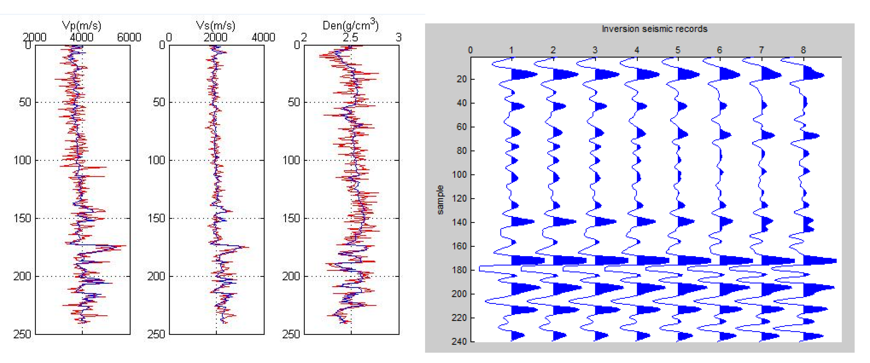
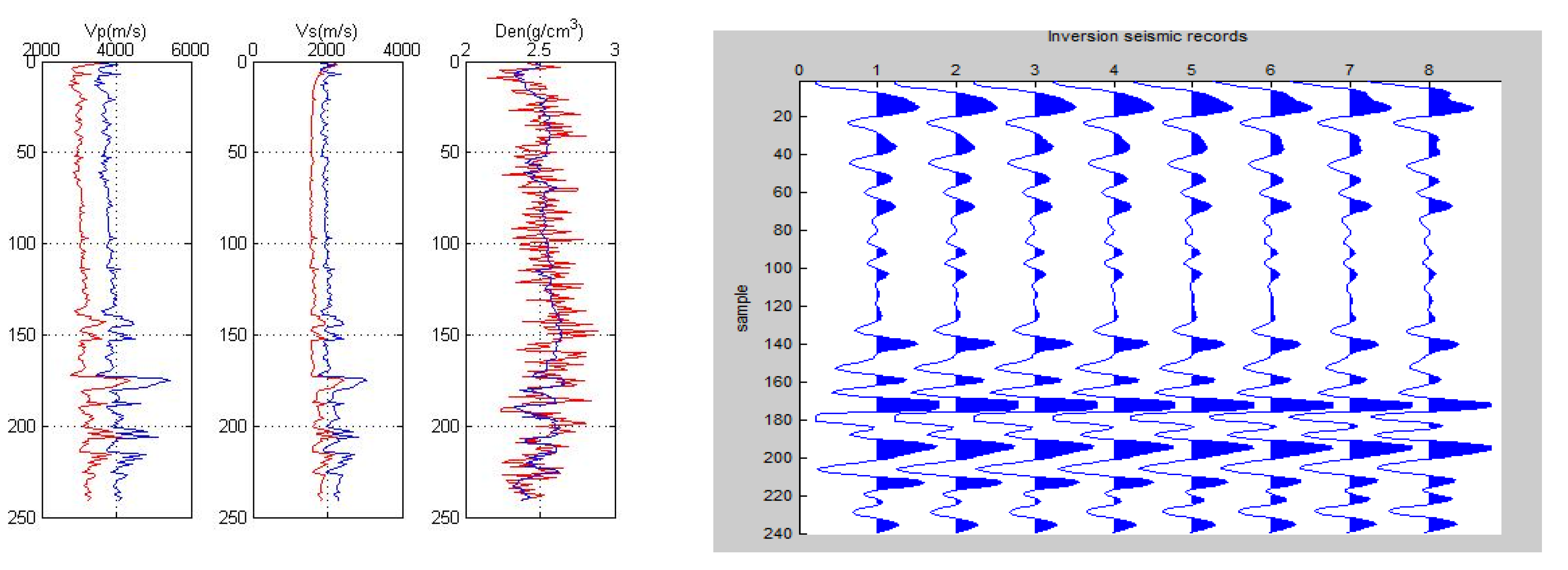
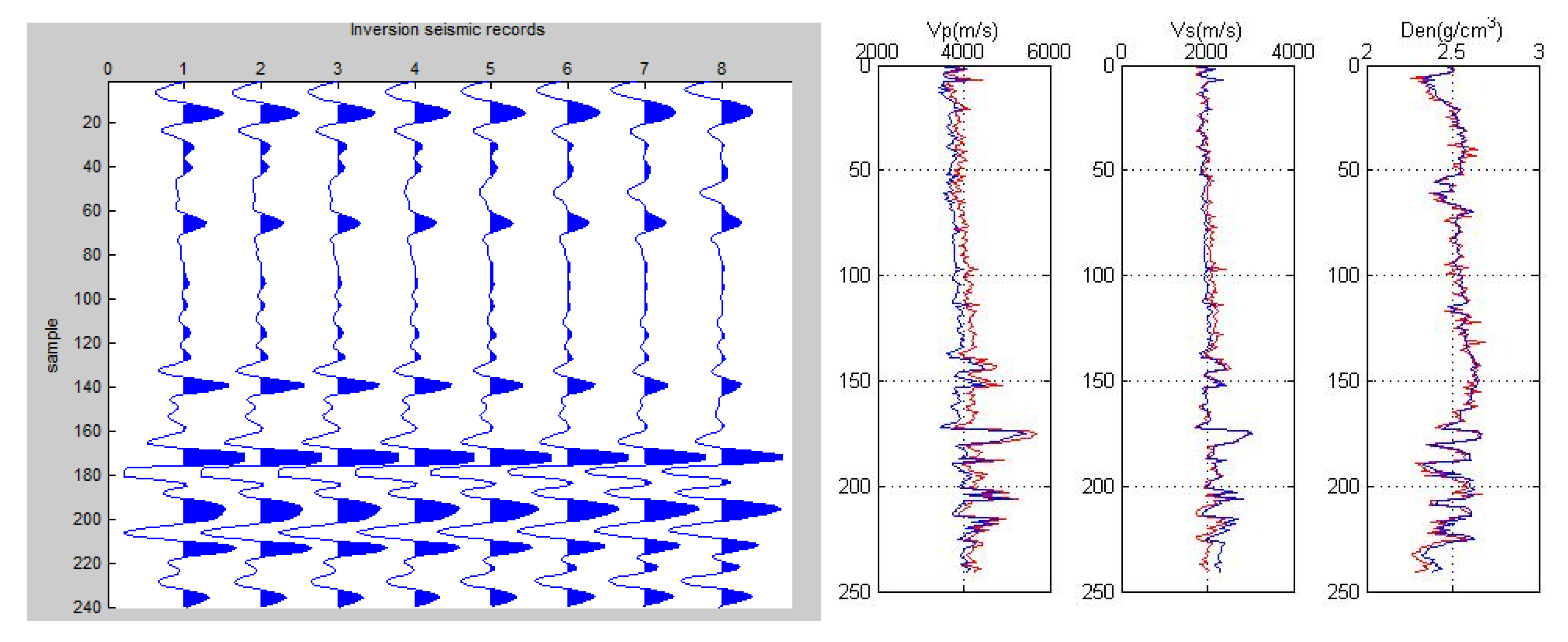
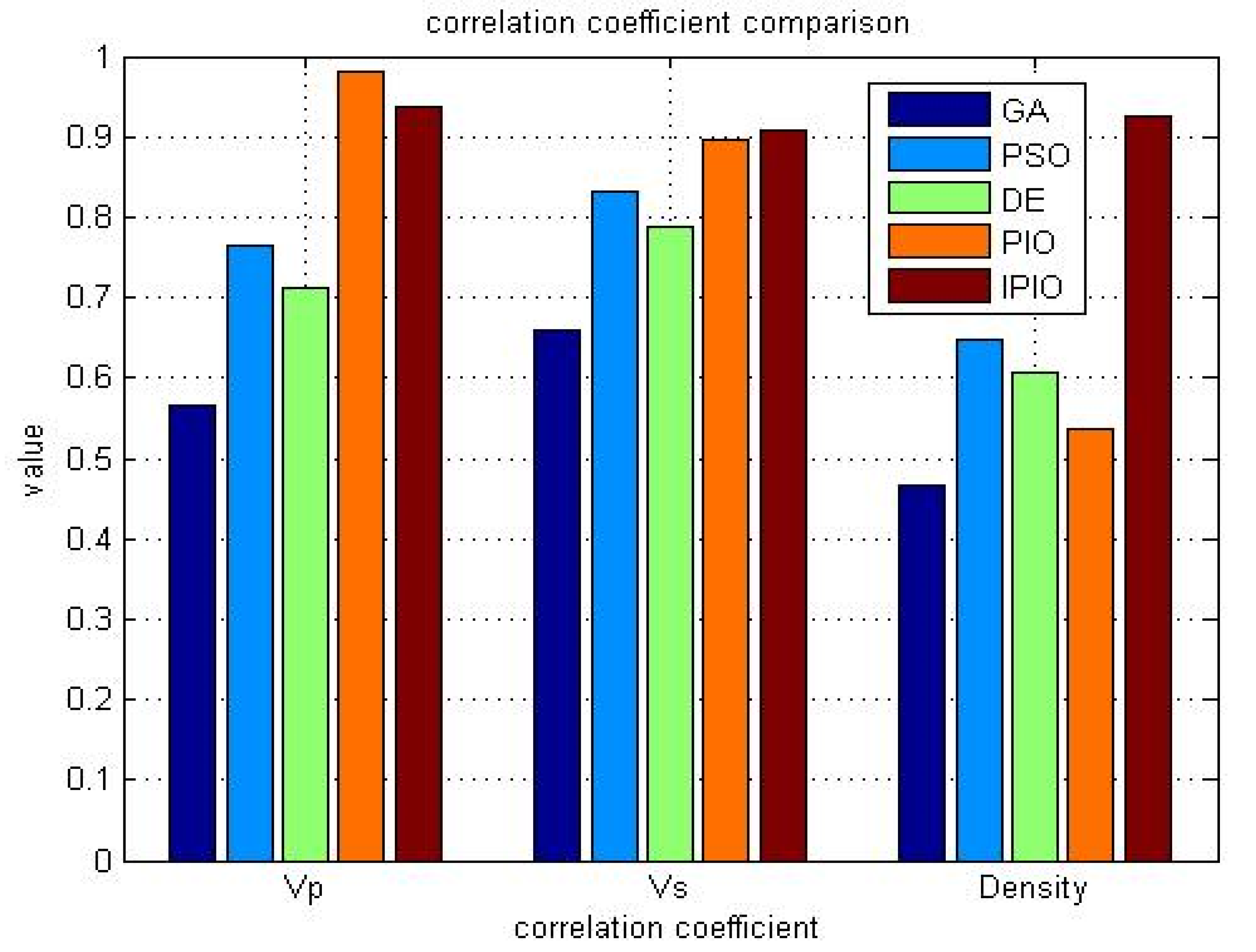
4.2. Simulation Experiment

The well-logging curve data in Dataset 1 are collected from 241 sampling points, including the p-wave velocity $V_p$, the S-wave velocity $V_s$, and the density $\rho$. At each sampling point, the data from eight different angles (0°, 6°, 11°, 17°, 23°, 29°, 34°, and 40°) were acquired and included in each dataset. The formula of Aki and Richard is used to forward the theoretical model of the logging curve, which is then used to calculate the reflection coefficient that is subsequently further convolved with the wavelet. When generating the seismic record data, it is necessary to use the relation between the upper and lower groups of sampling points. Therefore, the seismic record data contain 240 × 8 entries. The well-logging data thus generated are shown in Figure 2 and Figure 3.

The pre-stack AVO elastic parameter inversion was performed, respectively, using the proposed IPIO algorithm as well as the GA, PSO, DE and PIO algorithms. The experiments were conducted according to the algorithm parameter settings. The experimental results are shown in Figure 4, Figure 5, Figure 6, Figure 7 and Figure 8.

The mean correlation coefficients of the three parameters ($V_p$, $V_s$ and $\rho$) obtained from the experiments on the five algorithms (i.e., GA, PSO, DE, PIO and IPIO) are compared. The results are shown in Figure 9.

The comparison results shown in Figure 4, Figure 5, Figure 6, Figure 7 and Figure 8 and

Table 5. Comparison of the mean correlation coefficients of the three parameters for the five algorithms.

	GA	PSO	DE	PIO	IPIO
$V_p$	0.556364	0.765481	0.701792	0.980645	0.937951
$V_s$	0.650805	0.832094	0.787196	0.894879	0.908213
$\rho$	0.462346	0.649089	0.606702	0.537096	0.925746

indicate that the proposed IPIO algorithm significantly outperforms the GA, PSO, DE and PIO algorithms, with a drastically increased correlation coefficient. Form Table 5, it can be seen for the GA algorithm, the correlation coefficients for the three elastic parameters $V_p$, $V_s$ and $\rho$ are: 0.556364, 0.650805 and 0.462346. For the PSO algorithm, the correlation coefficients for the three elastic parameters $V_p$, $V_s$ and $\rho$ are: 0.765481, 0.832.94 and 0.649089. For the DE algorithm, the correlation coefficients for the three elastic parameters $V_p$, $V_s$ and $\rho$ are: 0.701792, 0.787196 and 0.606702. For the PIO algorithm, the correlation coefficients for the three elastic parameters $V_p$, $V_s$ and $\rho$ are: 0.980645, 0.894879 and 0.537096, but for the proposed algorithm, the correlation coefficients for the three elastic parameters $V_p$, $V_s$ and $\rho$ are: 0.937951, 0.908213 and 0.925746. The comparison results shown in Figure 9 indicate that the proposed IPIO algorithm effectively improves the correlation coefficients for the three elastic parameters $V_p$, $V_s$ and $\rho$, indicating that the inversed seismic data are closer to the actual seismic data.

The objective function values from the inversion are summarised in Figure 10. The original PIO algorithm has the worst performance in solving the inversion problem. The performance of the DE algorithm in solving the inversion problem is not satisfactory. GA outperforms the PIO and DE algorithms, with an objective function value of approximately 0.0035. The objective function value of the PSO algorithm is approximately 0.0018, which is better than the GA. The objective function value of the IPIO algorithm reaches 0.00094, which is an order of magnitude better than the other algorithms. The proposed IPIO algorithm greatly reduces the objective function value of the inversion. The comparison results in Figure 10 indicate that the proposed IPIO algorithm shows a rapid convergence rate and has a higher optimisation effectiveness than the GA, PSO and DE algorithms.

5. Conclusions

This study proposed an improved PIO algorithm that is more suitable for solving the inversion problem of pre-stack AVO elastic parameters. The proposed algorithm combines the PSO algorithm, the reverse particle, and the Gaussian factor, along with an improved initialisation strategy, to optimise the inversion, thus improving inversion accuracy. Through a large number of experiments, the authors confirm that the proposed IPIO algorithm is able to improve the accuracy of the inversion, making the inversed seismic data more consistent with the actual seismic data.

Future research directions can be divided into two levels: (1) At the algorithm level, more improvement strategies can be proposed for the PIO algorithm, so as to enhance the optimization ability of the algorithm; (2) At the problem level, the elastic parameters of the pre-stack seismic data inversion problem are complex. The actual cases and the geological structure are complex, from drilling to data acquisition. Each step has considerable errors. This article uses the data as an ideal data without error, and the actual situation, access to data, logging data and seismic data have some noise error. The inversion further increases the difficulty, and how to develop with noise error of pre-stack seismic data inversion of elastic parameters. Therefore, further research is needed.

References

1. Kennedy, J. Swarm Intelligence. Swarm Intelligence; Morgan Kaufmann Publishers Inc.: San Francisco, CA, USA, 2001. [Google Scholar]
2. Krause, J.; Ruxton, G.D.; Krause, S. Swarm intelligence in animals and humans. Trends Ecol. Evol. 2010, 25, 28–34. [Google Scholar] [CrossRef] [PubMed]
3. Dorigo, M.; Stützle, T. Ant Colony Optimization: Overview and Recent Advances. In Handbook of Metaheuristics; Springer: Cham, Switzerland, 2010. [Google Scholar]
4. Eberhart, R.; Kennedy, J. A New Optimizer Using Particle Swarm Theory. In Proceedings of the Sixth International Symposium, Nagoya, Japan, 4–6 October 1995; pp. 39–43. [Google Scholar]
5. Delice, Y.; Aydoğan, E.K.; Özcan, U.; İlkay, M.S. A Modified Particle Swarm Optimization Algorithm to Mixed-Model Two-Sided Assembly Line Balancing. J. Intell. Manuf. 2017, 28, 23–36. [Google Scholar] [CrossRef]
6. Chatterjee, S.; Sarkar, S.; Hore, S.; Dey, N.; Ashour, A.S.; Balas, V.E. Particle Swarm Optimization Trained Neural Network for Structural Failure Prediction of Multistoried RC Buildings. Neural Comput. Appl. 2017, 28, 2005–2016. [Google Scholar] [CrossRef]
7. Duan, H.; Qiao, P. Pigeon-Inspired Optimization: A New Swarm Intelligence Optimizer for Air Robot Path Planning. Int. J. Intell. Comput. Cybern. 2014, 7, 24–37. [Google Scholar] [CrossRef]
8. Duan, H.B.; Qiu, H.X.; Fan, Y.M. Optimal Combat Coordination Control for Unmanned Aerial Vehicle Using Predator-Escaped Pigeon. Chin. Sci. Technol. Sci. 2015, 45, 559–572. [Google Scholar]
9. Zhang, B.; Duan, H. Three-Dimensional Path Planning for Uninhabited Combat Aerial Vehicle Based on Predator-Prey Pigeon-Inspired Optimization in Dynamic Environment; IEEE Computer Society Press: Los Alamitos, CA, USA, 2017. [Google Scholar]
10. Dou, R.; Duan, H. Pigeon Inspired Optimization Approach to Model Prediction Control for Unmanned Air Vehicles. Aircr. Eng. Aerosp. Technol. Int. J. 2016, 88, 108–116. [Google Scholar] [CrossRef]
11. Duan, H.; Wang, X. Echo State Networks with Orthogonal Pigeon-Inspired Optimization for Image Restoration. IEEE Trans. Neural Netw. Learn. Syst. 2015, 27, 2413–2425. [Google Scholar] [CrossRef] [PubMed]
12. Sankareswaran, U.M.; Rajendran, S. A Novel Pigeon Inspired Optimization in Ovarian Cyst Detection. Curr. Med. Imaging Rev. 2016, 12, 43–49. [Google Scholar]
13. Lei, X.; Ding, Y.; Wu, F.X. Detecting Protein Complexes from DPINs by Density Based Clustering with Pigeon-Inspired Optimization Algorithm. Sci. China Inf. Sci. 2016, 59, 070103. [Google Scholar] [CrossRef]
14. Tizhoosh, H.R. Opposition-Based Learning: A New Scheme for Machine Intelligence. In International Conference on Computational Intelligence for Modelling, Control and Automation and International Conference on Intelligent Agents, Web Technologies and Internet Commerce (CIMCA-IAWTIC’06); IEEE: New York, NY, USA, 2005; pp. 695–701. [Google Scholar]
15. Zhang, S.; Duan, H. Gaussian Pigeon-Inspired Optimization Approach to Orbital Spacecraft Formation Reconfiguration. Chin. J. Aeronaut. 2015, 28, 200–205. [Google Scholar] [CrossRef]
16. Rodriguez-Zalapa, O.; Huerta-Ruelas, J.A.; Rangel-Miranda, D.; Morales-Sanchez, E.; Hernandez-Zavala, A. Csimfs: An Algorithm to Tune Fuzzy Logic Controllers. J. Intell. Fuzzy Syst. 2017, 33, 679–691. [Google Scholar] [CrossRef]
17. Alfonso, M.J.F.I.; Milán, D.P.S.; Córdoba, J.V.A.I.; Colmenero, N.P. Some Improvements on Relativistic Positioning Systems. Appl. Math. Nonlinear Sci. 2018, 3, 161–166. [Google Scholar] [CrossRef] [Green Version]
18. Plata, S.A.; Sáez, S.B. After Notes on Chebyshev’s Iterative Method. Appl. Math. Nonlinear Sci. 2017, 2, 1–12. [Google Scholar]
19. Neidell, N.S. Amplitude Variation with Offset. Lead. Edge 1986, 5, 47–51. [Google Scholar] [CrossRef]
20. Gao, W.; Zhu, L.; Guo, Y.; Wang, K. Ontology Learning Algorithm for Similarity Measuring and Ontology Mapping Using Linear Programming. J. Intell. Fuzzy Syst. 2017, 33, 3153–3163. [Google Scholar] [CrossRef]
21. Jin, J.; Mi, W. An Aimms-Based Decision-Making Model for Optimizing the Intelligent Stowage of Export Containers in a Single Bay. Discret. Contin. Dyn. Syst. Ser. S 2019, 12, 1101–1115. [Google Scholar] [CrossRef]
22. Wu, Q.; Zhu, Z.; Yan, X. Research on the Parameter Inversion Problem of Prestack Seismic Data Based on Improved Differential Evolution Algorithm. Clust. Comput. 2017, 20, 2881–2890. [Google Scholar] [CrossRef]
23. Yan, X.; Zhu, Z.; Wu, Q.; Gong, W.; Wang, L. Elastic Parameter Inversion Problem Based on Brain Storm Optimization Algorithm. Memet. Comput. 2019, 11, 143–153. [Google Scholar] [CrossRef]
24. Wu, Q.; Zhu, Z.; Yan, X.; Gong, W. An Improved Particle Swarm Optimization Algorithm for AVO Elastic Parameter Inversion Problem. Concurr. Comput. Pract. Exp. 2019, 31, 1–16. [Google Scholar] [CrossRef]
25. Yan, X.; Zhu, Z.; Hu, C.; Gong, W.; Wu, Q. Spark-Based Intelligent Parameter Inversion Method for Prestack Seismic Data. Neural Comput. Appl. 2018. [Google Scholar] [CrossRef]
26. Mallick, S. Model-based Inversion of Amplitude-variations-with-offset Data Using a Genetic Algorithm. Geophysics 1995, 60, 939–954. [Google Scholar] [CrossRef]
27. Priezzhev, I.; Shmaryan, L.; Bejarano, G. Nonlinear Multitrace Seismic Inversion Using Neural Network and Genetic Algorithm-Genetic Inversion. In Proceedings of the 3rd EAGE St. Petersburg International Conference and Exhibition on Geosciences-Geosciences: From New Ideas to New Discoveries 2008, Saint Petersburg, Russia, 2008. [Google Scholar]
28. Soupios, P.; Akca, I.; Mpogiatzis, P.; Basokur, A.T.; Papazachos, C. Applications of Hybrid Genetic Algorithms in Seismic Tomography. J. Appl. Geophys. 2011, 75, 479–489. [Google Scholar] [CrossRef]
29. Agarwal, A.; Sain, K.; Shalivahan, S. Traveltime and Constrained AVO Inversion Using FDR PSO. In SEG Technical Program Expanded Abstracts 2016; Society of Exploration Geophysicists: Tulsa, OK, USA, 2016; pp. 577–581. [Google Scholar]
30. Sun, S.Z.; Chen, L.; Bai, Y.; Hu, L.G. PSO Non-linear Pre-stack Inversion Method and the Application in Reservoir Prediction. In SEG Technical Program Expanded Abstracts 2012; Society of Exploration Geophysicists: Tulsa, OK, USA, 2012; pp. 1–5. [Google Scholar]
31. Sun, S.Z.; Liu, L. A Numerical Study on Non-linear AVO Inversion Using Chaotic Quantum Particle Swarm Optimization. J. Seism. Explor. 2014, 23, 379–392. [Google Scholar]
32. Zhou, Y.; Nie, Z.; Jia, Z. An Improved Differential Evolution Algorithm for Nonlinear Inversion of Earthquake Dislocation. Geod. Geodyn. 2014, 5, 49–56. [Google Scholar]
33. Song, X.; Li, L.; Zhang, X.; Huang, J.; Shi, X.; Jin, S.; Bai, Y. Differential Evolution Algorithm for Nonlinear Inversion of High-frequency Rayleigh Wave Dispersion Curves. J. Appl. Geophys. 2014, 109, 47–61. [Google Scholar] [CrossRef]
34. Lu, Y.F.; Bao, T.F.; Li, J.M.; Wang, T. Inversion of Geotechnical Mechanical Parameters Based on Improved Differential Evolution Algorithm Online Support Vector Regression and ABAQUS. J. Yangtze River Sci. Res. Inst. 2017, 34, 81–87. [Google Scholar]
35. Gao, Z.; Pan, Z.; Gao, J. Multimutation Differential Evolution Algorithm and Its Application to Seismic Inversion. IEEE Trans. Geosci. Remote Sens. 2016, 54, 3626–3636. [Google Scholar] [CrossRef]
36. Yan, X.; Zhu, Z.; Wu, Q. Intelligent Inversion Method for Pre-stack Seismic Big Data Based on MapReduce. Comput. Geosci. 2018, 110, 81–89. [Google Scholar] [CrossRef]
37. Aid, K.; Richards, P.G. Quantitative Seismology: Theory and Methods; W. H. Freeman and Co.: San Francisco, CA, USA, 1980. [Google Scholar]
Figure 1. The improved pigeon-inspired optimization (IPIO) algorithm flow chart.
Symmetry 11 01291 g001
Figure 2. Original logging curves.
Symmetry 11 01291 g002
Figure 3. Seismic records of theory model.
Symmetry 11 01291 g003
Figure 4. Logging curves and seismic records of inversion generated by basic genetic algorithm (GA).
Symmetry 11 01291 g004
Figure 5. Logging curves and seismic records of inversion generated by particle swarm optimisation (PSO).
Symmetry 11 01291 g005
Figure 6. Logging curves and seismic records of inversion generated by differential evolution (DE).
Symmetry 11 01291 g006
Figure 7. Logging curves and seismic records of inversion generated by pigeon-inspired optimisation (PIO).
Symmetry 11 01291 g007
Figure 8. Logging curves and seismic records of inversion generated by IPIO.
Symmetry 11 01291 g008
Figure 9. Comparison of the mean correlation coefficients of the three parameters for the GA, PSO, DE, PIO and IPIO algorithms.
Symmetry 11 01291 g009
Figure 10. Convergence curve of the algorithm.
Symmetry 11 01291 g010