Article

Research on a Real-Time Monitoring Method for the Wear State of a Tool Based on a Convolutional Bidirectional LSTM Model

Key Laboratory of Advanced Manufacturing Technology, Ministry of Education, Guizhou University, Guiyang 550025, China
*
Author to whom correspondence should be addressed.
Symmetry 2019, 11(10), 1233; https://doi.org/10.3390/sym11101233
Submission received: 14 August 2019 / Revised: 10 September 2019 / Accepted: 20 September 2019 / Published: 2 October 2019
(This article belongs to the Special Issue Symmetry in Mechanical Engineering)

Abstract

:
To monitor the tool wear state of computerized numerical control (CNC) machining equipment in real time in a manufacturing workshop, this paper proposes a real-time monitoring method based on a fusion of a convolutional neural network (CNN) and a bidirectional long short-term memory (BiLSTM) network with an attention mechanism (CABLSTM). In this method, the CNN is used to extract deep features from the time-series signal as an input, and then the BiLSTM network with a symmetric structure is constructed to learn the time-series information between the feature vectors. The attention mechanism is introduced to self-adaptively perceive the network weights associated with the classification results of the wear state and distribute the weights reasonably. Finally, the signal features of different weights are sent to a Softmax classifier to classify the tool wear state. In addition, a data acquisition experiment platform is developed with a high-precision CNC milling machine and an acceleration sensor to collect the vibration signals generated during tool processing in real time. The original data are directly fed into the depth neural network of the model for analysis, which avoids the complexity and limitations caused by a manual feature extraction. The experimental results show that, compared with other deep learning neural networks and traditional machine learning network models, the model can predict the tool wear state accurately in real time from original data collected by sensors, and the recognition accuracy and generalization have been improved to a certain extent.

Graphical Abstract

1. Introduction

As a critical component of intelligent manufacturing, mechanical intelligent fault diagnosis has become an essential part of “Made in China 2025” [1]. In mechanical processing, cutting is the most important means of manufacturing. At present, research in this field mainly focuses on tool cutting parameter optimization [2,3] and tool wear condition monitoring [4,5]. Real-time monitoring of the tool wear state is an essential part of the computerized numerical control (CNC) machining process in a manufacturing workshop. The wear state of a tool is affected by the processing procedures, workpiece materials, cutting parameters, and other factors. The whole system exhibits strong nonlinearity and uncertainty. The tool wear will not only reduce the processing quality of the CNC machining equipment but also affect the surface roughness and machining accuracy of the workpiece and seriously affect the overall stability and processing efficiency of the CNC machining equipment. The wear state of a tool will directly affect the machining accuracy, surface quality, and production efficiency of the parts. Therefore, the technology of tool condition monitoring (TCM) is of great significance for ensuring the quality of processing and realizing continuous automatic processing [6,7,8,9].
TCM methods are divided into direct measurement methods and indirect measurement methods. Direct measurement methods include resistance measurement methods, optical measurement methods, discharge current measurement methods, ray measurement methods, and computer image processing methods. The tool wear state can be obtained directly, but due to the influence of the coolant and other disturbances in the production process, the tool wear state in the mechanical processing stage cannot be detected in real time, which is rarely used in actual industrial production [10]. Indirect measurement methods include the cutting force measurement method, acoustic emission method, mechanical power measurement method, vibration signal and multi-information fusion detection [11,12,13,14,15]. Indirect measurement methods can acquire signals in real time through a sensor during tool cutting. After data processing and feature extraction, hidden Markov model (HMM), fuzzy neural network (FNN), back propagation neural network (BPNN), support vector machine (SVM), and other machine learning (ML) models can be used to monitor tool wear [16,17,18]. For example, Zhang Xiang et al. proposed micro-milling tool wear identification as the research object and established the HMM of tool wear. Eight optimal cutting forces were extracted as the HMM training input vectors by Fisher’s linear discriminant. The method can identify the micro-milling tool’s wear state with an accuracy rate of 85% [16]. X. Li et al. proposed an FNN designed and developed for machinery prognostic monitoring. The FNN is basically a multi-layered fuzzy-rule-based neural network that integrates a fuzzy logic inference into a neural network structure. This method is helpful to accelerate the learning process of the complex conventional neural network structure, and the accuracy in prediction and rate of convergence are better than those of similar ML models [17]. Liao Zhirong et al. proposed a tool wear condition monitoring system based on acoustic emission technology. By analysingrepresentative acoustic signals, the energy ratios from six different frequency bands are selected from the time–frequency domain. These are used as a classification feature to determine the amount of tool wear. In this method, the SVM is used as the classification method, which can ultimately achieve an accuracy rate of 93.3% [18]. The traditional ML model adopts shallow learning. Since ML is affected by the quality instability of the manual extraction feature, a random initialization of the weights can easily enable the objective function to converge to the local minimum. When the number of layers is too large, the forward propagation of the residuals will be lost, leading to gradient diffusion. At the same time, ML is limited by the inability to capture the dependence of long-distance signals on the sequential input. Deep learning (DL) can effectively avoid these problems.
DL was first introduced into machine learning (ML) in 1986 and then used in an artificial neural network (ANN) [19] in 2000. DL uses multi-level non-linear information to process low-level features to form more abstract high-level representations for supervised or unsupervised feature learning, representation, classification, and pattern recognition [
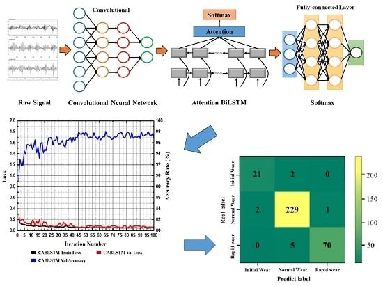
20]. The DL model is an “end-to-end learning” model, which does not require complex data pre-processing of the original data, making the construction of the model more concise (Figure 1). At present, the DL method has emerged in the industrial field. DL models represented by a CNN have been gradually applied to the study of tool wear condition monitoring and achieved specific results [21,22,23]. For example, Zhang Cunji et al. proposed transforming the vibration signal of a tool in the process of machining into an energy spectrum by a wavelet packet transform (WPT) and inputting the spectrum into a CNN to extract the features automatically and classify them accurately [21]. German Terrazas et al. proposed that based on the gramian angular summation fields (GASF) module, a large number of continuous force signals generated by cutting tools in a high-speed milling process can be automatically converted into two-dimensional images, which are input into a CNN to obtain the tool wear status [22]. Cao Dali et al. proposed the construction of a DenseNet using the dense connection, which adaptively extracts hidden high-dimensional features from original time series signals. The results showed that deepening the network layers is helpful for improving the accuracy of the tool wear monitoring model [23]. The above methods adopt DL to extract features adaptively, which basically solves the shortcoming of a manual extraction of the signal features. However, the convolution neural network (CNN) used relies too heavily on high-dimensional feature extraction. The excessive number of convolutional layers is prone to gradient dispersion, and the number of convolutional layers is too small to grasp the global features and does not take into account the critical feature of the correlation between the timing signal samples generated during tool processing.
Therefore, this paper proposes a method for real-time monitoring of a tool wear state based on a CNN and bidirectional long short-term memory (BiLSTM) network model with an attention mechanism (CABLSTM). The sensor acquires the signals generated during tool processing in real time, which are directly fed into the CNN for parallel local feature extraction and then into the BiLSTM network for feature extraction of the long-distance dependence information. The attention mechanism is used to calculate the network weights and distribute them reasonably. Finally, the signal feature information with different weights is sent to a Softmax classifier to classify the tool wear status, avoiding the complexity and limitation caused by a manual feature extraction. This method can meet the real-time and accuracy requirements of tool monitoring in actual industrial production.
The remainder of this paper is organized as follows. Section 2 presents the CABLSTM algorithm. Section 3 presents the monitoring process of tool wear. Section 4 presents the experimental results of the tool wear condition monitoring. Section 5 concludes the article.

2. CABLSTM Model

Inspired by the literature [24], this paper applied a CNN and recurrent neural network (RNN) fusion to the real-time monitoring task of a tool wear state, constructs two network models of convolutional long short-term memory (CLSTM) and convolutional bi-directional long short-term memory (CBLSTM), effectively solves the problem of the correlation between the ignored time-series signals in a single CNN, and avoids the problem of gradient dispersion and gradient explosion in a circular neural network. Meanwhile, the attention mechanism is introduced on the basis of the CBLSTM network. Finally, the CABLSTM network is proposed, which further improves the accuracy of model prediction.
The CABLSTM model mainly includes four parts: The first part involves the local feature extraction of the single time step timing signal, which mainly uses a one-dimensional CNN for neighborhood filtering, uses a sliding window for the convolution calculation, and finally obtains the high-dimensional features of the single time step timing signal. The second part involves the extraction of the time series of time-series signals, and the BiLSTM network is used to process the high-dimensional features generated by the continuous time step timing signals and gradually synthesize the vector feature representation of the input signals. The third part uses the attention mechanism to calculate the importance distribution of sequential signal features in continuous time steps and generate the feature model of sequential signals with an attention probability distribution. The fourth part is the classifier, which uses dropout technology to prevent overfitting and uses the Softmax classifier to predict the tool wear states. The neural network framework for real-time monitoring of the tool wear state based on CABLSTM is shown in Figure 2.

2.1. Local Feature Extraction of Single Time Step Timing Signals

The one-dimensional CNN can be applied to a time-series analysis of sensor data [24,25,26]. In the one-dimensional convolutional layer, multiple filters are used to perform neighborhood filtering of the input time-series data, and the acquired feature maps are superimposed to form an output feature map of the convolutional layer. Then, the pooling layer extracts the fixed-length feature vectors from feature maps of each candidate frame for a feature dimension reduction, thereby extracting critical features in the time-series data and simplifying the complexity of the network calculation.
In this paper, a one-dimensional CNN was used to directly process the timing signals generated during tool processing. The CNN includes two layers: A convolutional layer and a pooling layer. The convolution layer performs neighborhood filtering of the time-series signals of each dimension using a one-dimensional convolution operation to generate feature maps, and each feature map can be regarded as a convolution operation of different filters on the current time step timing signals [27]. When the input timing signal is x , the weight vector of the convolution kernel is w , the total number of samples is m , the size of the convolution kernel is n , is the convolution operation, and the output feature map of the convolutional layer y can be expressed as follows:
y = x w = m = 0 m x ( m ) w ( n m ) .
In the convolutional layer, each neuron of the l layer is only connected to a local window neuron in the l 1 layer to form a local connection network. The calculation formula for the one-dimensional convolution layer is as follows:
x j l = f ( i M j x i l 1 w i j l + b j l ) ,
where x j l is the j feature map of the l layer, f ( · ) is the activation function, M j is the input feature vector, x i l 1 is the i feature map of the l 1 layer, w i j l is a trainable convolution kernel, and b j l is the bias parameter. Considering the convergence speed and overfitting problems, the rectified linear unit (Relu) is chosen for the non-linear activation function, which converges faster to improve the sparsely of the network in this paper, reduces the interdependence of the parameters, and alleviates the occurrence of overfitting. The formula for the Relu activation function is as follows:
a i ( l + 1 ) ( j ) = f ( y i l + 1 ( j ) ) = max { 0 , y i l + 1 ( j ) } ,
where y i l + 1 ( j ) is the output value of the volume and operation and a i l + 1 ( j ) is the activation value of y i l + 1 ( j ) .
The convolutional layer is connected to the pooling layer for the local maximum or local mean, namely, max pooling and mean pooling [28]. The pooling layer has the function of feature selection, which can ensure that the feature can resist a deformation; at the same time, the pooling layer can reduce the feature dimension, speed up the network training, reduce the number of parameters, and improve the robustness of the feature. In this paper, max pooling was used to obtain the maximum value of the feature points in the neighborhood. The formula is as follows:
P i l + 1 ( j ) = max ( j 1 ) W + 1 t j W { q i l ( t ) } ,
where q i l ( t ) is the value of the t neuron in the i feature vector of the l layer and t [ ( j 1 ) w + 1 , j w ] . w is the width of the pooled region, and P i l + 1 ( j ) is the value corresponding to the l + 1 layer neuron.
The one-dimensional CNN performs the feature extraction of the original data, and the three-dimensional features of the time-series signal are better expressed as high-dimensional features, which facilitate the subsequent time-series feature extraction of the BiLSTM network. The basic structure of the one-dimensional CNN is shown in Figure 3.

2.2. Time-Series Feature Extraction of Time-Series Signals

Long short-term memory (LSTM) is an exclusive self-connected recurrent neural network (RNN). LSTM introduces a gate function to generate the path of continuous gradient flow for a long time, which effectively avoids the problem of gradient disappearance and gradient explosion caused by the chain rule in the gradient calculation of hidden layers in RNN [29]. LSTM can mine the temporal variation law of relatively long intervals in time series, and it is particularly used to process time-series data. The original signal generated during tool processing has a timing relationship. The LSTM network can encode the time series of time-series signals and mine the timing variation in relatively long intervals in the time series [30]. To ensure that the real-time monitoring model of tool wear can better learn the dependence of time-series features between time-series signals and improve the accuracy of the model classification, this paper improves the existing LSTM network [31] and builds a BiLSTM network with a symmetric structure by constructing two directions of LSTM networks [32]. At the same time, the attention mechanism is introduced into the BiLSTM network to increase the attention layer, which enables the model to both extract temporal signal features from both the positive and negative directions and selectively learn the critical information of the signal features.
The constructed BiLSTM network contained 256 neurons in this paper. The forward and reverse LSTM networks consisted of 128 neurons. Each BiLSTM neuron included an input gate, a forget gate and an output gate, which are represented by i , f , and o , respectively. The internal structure of the BiLSTM neurons is shown in Figure 4.
The input gate i is used to control the amount of current input information x t of the network that can be saved to the memory unit C t , uses the sigmoid function to determine new information to be saved, uses the tanh function to generate a new candidate vector C ˜ t , and sends the information to be saved to the memory. The unit completes the update. The forget gate f is used to control the self-connecting unit, filters the information in the memory unit C t 1 at the previous moment to determine the amount of valid information that needs to be retained in the current memory unit C t , and forgets the useless information. The output gate o controls the influence of the memory unit C t on the current output value h t and determines the amount of information that the memory unit C t outputs at time step t . The formula is as follows:
i t = σ ( W x i x t + W h i h t 1 + b i ) ,
C ˜ t = tanh ( W x c x t + W h c h t 1 + b c ) ,
f t = σ ( W x f x t + W h f h t 1 + b f ) ,
C t = f t c t 1 + i t C ˜ t ,
o t = σ ( W x o x t + W h o h t 1 + b o ) ,
h t = o t tanh ( C t ) ,
where C is the memory unit, which is called the cell state, C t is the memory cell state at time step t , C ˜ t is the candidate vector of the memory cell at time step t , x t is the input vector at time step t , h t is the output vector at time step t , W is the weight vector of the network, b is the offset vector, represents a multiplication of vector elements, σ ( · ) is the sigmoid function, and the tanh function is the hyperbolic tangent activation function.
The high-dimensional feature of the input timing signal is outputted by the forward LSTM network vector h t , the inverse LSTM network output vector is h t , and the BiLSTM network output eigenvector is P t at time step t . The formula is as follows:
h t = L S T M ( h t 1 , x t , C t 1 ) .
h t = L S T M ( h t + 1 , x t , C t + 1 ) .
P t = [ h t , h t ] .
In this paper, the attention mechanism was used to assign weights to each time step output vector of the BiLSTM layer by assigning different initialization probability weights. Finally, the values were calculated by the sigmoid function. The attention mechanism achieves selective filtering and focusing of some critical information from a large number of signal features. The focusing process was embodied in the calculation of the weight coefficients. Different weights were allocated to different critical pieces of information, and the proportion of critical information was enhanced by lifting the weights to reduce the loss of critical information of long sequence timing signals. The calculation formula for the attention mechanism [30] is as follows:
u t = tanh ( W s P t + b s ) ,
α t = s o f t max ( u t T , u s ) ,
ν = α t P t ,
where P t is the output eigenvector of the BiLSTM layer at time step t , u t is the hidden layer representation of P t through the neural network layer, u s is the randomly initialized context vector, α t is the importance weight of u t normalized by the Softmax function, and v is the feature vector of the final text message. u s is generated randomly during the training process, and finally, the output value v of the attention layer is mapped via the Softmax function to obtain a real-time classification result of the tool wear state. The partial expansion of the BiLSTM network model with the attention mechanism along the time axis is shown in Figure 5.

2.3. Network Model Training

In this paper, dropout technology was introduced into the real-time monitoring model of the tool wear state to prevent the model from overfitting during training. The activation function of the network model uses Softmax, and the loss function uses Categorical_crossentropy, which was used to classify the wear features of the acquired time-series signals. The formula is as follows:
y = s o f t max ( v ) = e v i m = 1 M e v m .
y is a vector whose dimensions are the number of categories, each of which has a value between [0,1], and the sum of all dimensions is 1, which is the probability that the tool wear state belongs to a category. M is the number of possible categories. During the training of the model, the entire model was trained by the Categorical_crossentropy loss. The calculation formula for the cross-entropy error is as follows:
l o s s = i = 1 n y ^ i 1 log y i 1 + y ^ i 2 log y i 2 + + y ^ i m log y i m ,
l o s s y i 1 = i = 1 n y ^ i 1 y i 1 ,
l o s s y i 2 = i = 1 n y ^ i 2 y i 2 ,
l o s s y i m = i = 1 n y ^ i m y i m ,
where m is the number of classifications, n is the number of samples, y ^ i m is the i value in the tool wear state real category label vector, and y i m is the i value of the output vector y of the Softmax classifier. For the obtained cross-entropy error, the average was taken as the loss function of the model. The Adam method was used to minimize the objective function when training the model. The Adam method is essentially the RMSprop method with a momentum term. The Adam method dynamically adjusts the learning rate of each parameter by using a first-order moment estimation and a second-order moment estimation of the gradient. The main advantage of the Adam method was that after the offset correction, the learning rate of each iteration had a specific range, which makes the parameter change relatively stable.

3. Real-Time Monitoring Method of the Tool Wear State

An acceleration sensor is used to collect the vibration signal generated by a computerized numerical control (CNC) machining device in the process of machining the workpiece in real time. The input signal of the real-time monitoring model of the tool wear state is the α x , α y , and α z vibration signals, and the output of the model is the predicted value of the tool wear state. In this paper, after continuous sampling of the original vibration signal generated by each milling cutter feed, the sampling points with a length of 2000 were cut to form multiple tensors (3 × 2000), which were taken as the input data of the model for the DL neural network. The schematics diagram of the CABLSTM network is shown in Figure 6. The CBLSTM network did not have an attention block, while the CLSTM network was similar to the CBLSTM network but with an LSTM block instead of a BiLSTM block.
The input data of the CABLSTM network included the time-series signal (data type) and the wear classification (label type). The feature extraction and expression of the time-series signal were achieved by two convolution layers, one pooling layer, one flatten layer, one BiLSTM layer, one attention layer, and two fully-connected layers. The parameters of each layer of the network are shown in Table 1.

4. Experimental

4.1. Experimental Design

A real-time monitoring system for the tool wear state includes a condition monitoring facility and a data analysis unit. The condition monitoring facilities include the basic equipment used to process the workpiece, the equipment to collect the vibration signals generated during the processing, and the equipment to measure the value of tool wear. The data analysis facility included high-performance computers and DL platforms for analyzing and processing the data and classifying and reporting the tool wear status in real time.

4.1.1. Condition Monitoring

The experimental platform of this paper was provided by the Engineering Training Center of Guizhou University. A high-precision CNC vertical milling machine (Model: VM600) was used for the milling workpiece. No coolant was added during milling. The workpiece was milled steel (S136). The milling tool had a cemented carbide 4-edge milling cutter, and its surface was covered with layers of a titanium aluminum nitride coating. The diameter of the tool was 6 mm, the rake angle was 4°, the clearance angle was 8°, and the helix angle was 30°. The cutting parameters of the milling experiment are shown in Table 2.
In the experiment, three accelerometers (Model: INV9822; Range: ±50 g) were magnetically attracted to the machine tool fixture in the x , y , and z directions for real-time acquisition of the original vibration signals generated during tool machining. A high-precision digital acquisition instrument (model: INV3018CT) from the Beijing Oriental Institute of Vibration and Noise was used to process the real-time signals and transmit them to a computer. The sampling frequency of the signal was 20 kHz, 200 mm of milling in each direction of the tool was recorded as a milling stroke, and each tool was milled for 330 strokes. After each milling stroke, the milling cutter was removed from the milling machine and photographed. A pre-calibrated high-precision digital microscope (EVDM-101) was used for the measurement, the optical magnification was 0.7×–4.5×, the electronic magnification was 35×–235×, and the measuring accuracy was 0.1 μm. During the measurement process, the position of the wear zone of the minor flank surface of the milling cutter, which was the most easily worn, was selected as the measurement position, and the same reference line was taken as the standard to ensure that the position remains unchanged during the measurement. The wear value (VBmax) was calculated by subtracting the current cutting edge length from the initial length of the cutting edge of the milling cutter. The real-time monitoring experimental device of the tool wear state is shown in Figure 7.

4.1.2. Data Analysis

The DL hardware platform of the experiment used high-performance servers: An Intel Xeon E5-2650 processor, with a frequency of 2.3 GHz, 256 GB of memory, and an NVIDIA GeForce TITAN X graphics processing unit (GPU). The software platform used the Ubuntu 16.04.4 operating system with Keras as the front-end of the in-depth learning framework and TensorFlow as the back-end for data analysis.
The milling operation was carried out with four milling cutters (C1, C2, C3, and C4). Each milling cutter was performed 330 times, and 1320 original signal samples were obtained. The data of three milling cutters (C1, C2, and C3) were used for the training set and verification set of the model, and one milling cutter (C4) data was used for the test set of the model. The training set was used for model fitting the data samples, the verification set was used for adjusting the hyperparameters of the model, the initial ability of the model was evaluated, and the test set was used to evaluate the generalization ability of the final model. In the DL training process, a sufficient number of samples were needed to improve the learning quality of the neural network. The data samples of the original processed signals were long sequences of periodic timing signals. According to the principle of signal sampling, in this paper, 100,000 points of each sample were sampled continuously, and 50 short sequence timing signals with a length of 2000 were cut to be used for model input after data normalization to reduce the computational intensity of the network training. At the same time, data expansion could increase the experimental data based on the original magnitude data, improve the robustness of the network, and reduce the risk of overfitting.
The processing conditions in the experiment had the following characteristics: 1. Finishing milling and small back engagement were performed; 2. the workpiece was milled steel (S136) with high hardness after heat treatment; and 3. the experiment needed to produce tool data set quickly and accurately. This paper referred to references [33,34,35] and the measurement methods of milling tool wear in 2010 prognostics and health management (PHM) competition. The following method was used as the blunt standard for the milling cutter in this experiment: The maximum value (VBmax) of the wear zone of the minor flank surface of the milling cutter was selected as the quantified value reflecting the wear state. It was specified that failure of the milling cutter occurred when the wear value of the milling cutter was greater than 0.13 mm. The wear process of the milling cutters (C1, C2, C3, and C4) is shown in Figure 8.
Each sample contains three-dimensional vibration signals and the wear values of the four rear blades. To prevent mutual interference of the different blade wear values, the maximum wear value of the four blades was selected as the label of the milling stroke. The wear state of the tool was divided into initial wear, normal wear, and rapid wear. In this paper, the wear state of the tool was defined according to the actual wear curve of each milling cutter. The actual wear curve was used to determine the wear degree of the tool. The tool wear degree was divided into three types of label data, and the label data were converted by a one-hot coding form to facilitate the classification of the final tool wear state. The classification of the final tool wear state is shown in Table 3.

4.2. Comparison of the Experimental Results of the Deep Learning Model

The original signal generated by the milling process was sampled and then sent to the DL neural network model. The model adaptively extracted the high-dimensional features implied in the time-series signal and calculated the actual output value and reality of the model. The Adam algorithm reduced the error distance between the values, and the network weight was continuously updated so that the actual output value of the model was closer to the real value. To further verify the performance of the proposed algorithm, we implemented the bearing fault diagnosis algorithm of the CNN model in [25] and the turbofan engine life prediction algorithm of the BiLSTM model in [26]. The above model was compared with our proposed CLSTM, CBLSTM, and CABLSTM networks. The five training models used the same training parameters. The specific training parameters of the model are shown in Table 4.
After the training and verification of the DL neural network, different loss function values and accuracies were obtained. The loss function values of the CNN [25], BiLSTM [26], CLSTM, CBLSTM, and CABLSTM models and the accuracy of the verification set are shown in Figure 9, Figure 10, Figure 11, Figure 12 and Figure 13, where the x axis was used to represent the number of iterations of the milling data set, and the double y axis was used to represent the loss function value and the model verification accuracy.
It can be concluded from the figure that the loss function value of the network model training set decreased with an increase in the number of iterations and finally stabilized. The loss function value of the verification set fluctuated periodically, and the loss function of the CLSTM model had a large amplitude. The CNN, BiLSTM, CBLSTM, and CABLSTM models were relatively stable, the overall trend of the loss function was decreasing and finally converging, there was no gradient explosion or dispersion phenomenon, and the network convergence speed was faster. The accuracy rates of the CNN and BiLSTM model validation sets were 87.57% and 86.36%, respectively, and the prediction accuracy was low. This result indicates that the individual DL network could predict the tool wear state, but deeper features could not be captured due to the limitation of the network model capability. There were deeper features hidden in the tool vibration signal. The network model proposed in this paper was superior to the CNN and BiLSTM network. This is because the network structure was relatively deep, which is conducive to mining deeper features. First, the CNN was used to extract the local features of the timing signals, which could effectively filter the noise in the original signal. At the same time, the length of the timing signal was reduced, which facilitates subsequent network learning depending on the time-series characteristics of the time-series signals and improved the ability of the model prediction.
In the network model proposed in this paper, the CABLSTM model had the best performance, which ewas superior to that of the CLSTM and CBLSTM models, and achieved high prediction accuracy. The initial prediction accuracy of the CLSTM model was relatively low. After 65 iterations, the accuracy of the verification set was basically stable and above 96%, and the accuracy was 96.42% after 100 iterations. The CBLSTM model used a two-way LSTM network to access past and future information; that is, it could extract timing signal features from both the forward and reverse directions and extract more abundant information features. After 42 iterations, the accuracy rate of the verification set was basically stable at over 96%, and the accuracy rate was 97.04% after 100 iterations. The CABLSTM model introduced the attention mechanism on the basis of CBLSTM, which selectively filtered out some key information from a large amount of information and focused on the key information, reducing the loss of key information features of long sequence texts. After 35 iterations, the accuracy of the verification set was basically stable and above 96%, the accuracy was 97.50% after 100 iterations, the loss function value reached 0.0651, and the network stability was higher. The loss function and the accuracy of the verification set and test set are shown in Table 5.
The data of the milling cutter (C4) were selected as the test set of the DL network model to evaluate the generalization ability of the final model. The total number of test samples was 330, including 23 initial wear samples, 232 standard wear samples, and 75 sharp wear samples. The samples were randomly fed into the trained DL network model. The CABLSTM model had high precision and recall. The F1-score reaches the optimum value at 1 (perfect precision and recall), and the worst is 0. The F1-score in this paper was 0.9697. The evaluation indices of the CABLSTM model are shown in Table 6. The test results show that the CABLSTM model proposed in this paper hade a strong generalization ability. Although the test time was not as good as that of the partial comparison model, the algorithm found a good balance between time and precision.
It can be concluded from the figure that the CABLSTM model proposed in this paper completed the inspection of the milling cutter (C4) with an accuracy of 96.97%. The predicted results of normal wear were more accurate. There were some deviations between the initial wear and sharp wear, but the deviations were within a reasonable range. The incorrect prediction results mainly occurred in the transition stage of the wear degree. This is because the tool was in the normal wear state for a long time during the machining process, the amount of data that could be learned by the model was relatively large, and the features were relatively distinct; in addition, the tool had a short period of initial wear and rapid wear, and the amount of data that could be obtained was insufficient. The confusion matrix of the wear test results of the tool test set is shown in Figure 14.
When the real-time monitoring system of tool wear state was working, the acceleration sensors would bring a three-axis vibration signal of length 2000 to the monitoring model of the CABLSTM network. The model performed a forward calculation to identify the current tool wear state and achieve real-time monitoring of the tool wear state.

4.3. Comparison of Deep Learning and Machine Learning

To further validate the feasibility of the proposed model, a comparative experiment was designed with alternative ML models. The same data set used for DL was used in the experiment. More specifically, the commonly used models in traditional tool wear value detection approaches, including the BPNN, the SVM, the HMM, and the FNN, were compared with the CABLSTM model proposed in this paper. The wavelet threshold denoising method was used to perform noise reduction processing on the original signal collected by the acceleration sensor. The data features of the time domain, frequency domain, and time-frequency domain were extracted, and the specific extraction method is shown in Table 7. Pearson’s correlation coefficient (PCC) was used to reflect the correlation between the feature and the wear value, and the feature with a correlation coefficient greater than 0.9 was selected as the extraction object to achieve a feature dimensionality reduction. The extracted features were used as the input of the ML model.
It can be concluded from Table 7 that the accuracy of traditional ML models varied greatly, which was due to the instability of the artificial extraction features, and the construction of the model would have an impact on the prediction results. The DL model proposed in this paper could achieve ideal results by adaptively extracting hidden high-dimensional features and reasonable network depth design for tool processing signals without data pre-processing. The prediction accuracy was significantly higher than that of the BPNN, SVM, and HMM. However, the prediction accuracy of the FNN reached 94.24% because the FNN used a neural network to learn the rules of the fuzzy system. According to the learning sample of the input and output, the design parameters of the fuzzy system were automatically designed and adjusted to realize the self-learning and adaptive functions of the fuzzy system. Compared with the other algorithm models, this method demonstrated a great improvement in performance. The test sample speed of the CABLSTM model could reach 6 ms, which could meet the requirements of real-time tool wear monitoring in industrial production. The accuracy of ML and DL prediction is shown in Table 8.

5. Conclusions

In this paper, we proposed the application of a CNN and RNN fusion to real-time monitoring of a tool wear state and modified the network parameters and structure according to the characteristics of vibration signals to monitor the tool wear degree in real time. The prediction accuracy of the CBLSTM reached 96.97%. In the pre-processing stage, the wear state of the tool was defined according to the actual wear curve, which was used to determine the wear degree of the tool and improve the accuracy of the data label classification. At the same time, the experimental data were added to the original magnitude data to improve the robustness of the algorithm by employing the data expansion method. A one-dimensional CNN was used to extract the local features, and abundant high-dimensional features were extracted from the original signal, which avoided the limitation of the traditional manual feature extraction, better characterizede the hidden tool wear state information in the original signal, and shortened the network model training time. The idea of introducing the attention mechanism was innovatively applied to the improved CBLSTM network model, which effectively improved the recognition accuracy and generalization performance of the real-time monitoring. The experimental results show that the CABLSTM model had certain advantages in the real-time monitoring of tool wear, which could meet the industrial requirements in terms of recognition accuracy and recognition speed.
In the process of actual manufacturing, the processing procedures and site conditions were often complicated and variable. There were many features that could reflect the wear state of a tool. In this paper, the original signal collected by the acceleration sensor was used as the tool wear monitoring index, which was restricted by the training data volume and processing method. It might not be applicable to meet the requirements of arbitrary working conditions. In future work, multi-source data fusion technology and DL theory will be used to further study the information characterizing the wear state of the tool, improve the proposed method, and extend the method to industrial monitoring.

Author Contributions

Q.C. and Q.Y. conceived and designed the experiments; Q.C. and Y.L. performed the experiments; Q.C. and H.H. analyzed the data; Q.C. wrote the paper; Q.Y., Q.X., and Q.C. revised and polished the manuscript. All authors have read and approved the final manuscript.

Funding

This research was funded by the Guizhou Province Science and Technology Fund Project (Branch Support [2017] 2870), and Guizhou Province Education Department Science and Technology Talents Support Project (Branch Support KY [2017]062).

Acknowledgments

We gratefully acknowledge the support of NVIDIA Corporation with the donation of the Titan X GPU used for this research.

Conflicts of Interest

The authors declare no conflict of interest.

References

  1. Lei, Y.G.; Jia, F.; Kong, D.T.; Lin, J.; Xing, S.B. Opportunities and Challenges of Machinery Intelligent Fault Diagnosis in Big Data Era. J. Mech. Eng. 2018, 54, 94–104. [Google Scholar] [CrossRef]
  2. Mia, M.; Królczyk, G.; Maruda, R.; Wojciechowski, S. Intelligent Optimization of Hard-Turning Parameters Using Evolutionary Algorithms for Smart Manufacturing. Materials 2019, 12, 879. [Google Scholar] [CrossRef] [PubMed]
  3. Andres, B.; Gorka, U.; Jose, M.P.; Octavio, M.P.; Luis, N.L. Smart optimization of a friction-drilling process based on boosting ensembles. J. Manuf. Syst. 2018, 48, 108–121. [Google Scholar]
  4. Zhu, K.P.; Zhang, Y. A generic tool wear model and its application to force modeling and wear monitoring in high speed milling. Mech. Syst. Signal Process. 2018, 115, 147–161. [Google Scholar] [CrossRef]
  5. Benkedjouh, T.; Zerhouni, N.; Rechak, S. Tool wear condition monitoring based on continuous wavelet transform and blind source separation. Int. J. Adv. Manuf. Technol. 2018, 97, 3311–3323. [Google Scholar] [CrossRef]
  6. Zhou, Y.Q.; Xue, W. Review of Tool Condition Monitoring Methods in Milling Processes. Int. J. Adv. Manuf. 2018, 96, 2509–2523. [Google Scholar] [CrossRef]
  7. Beranoagirre, A.; Urbikain, G.; Marticorena, R.; Bustillo, A.; Lacalle, L. Sensitivity Analysis of Tool Wear in Drilling of Titanium Aluminides. Metals 2019, 9, 297. [Google Scholar] [CrossRef]
  8. Krahmer, D.M.; Hameed, S.; Egea, A.J.; Pérez, D.; Canales, J.; Lacalle, L.N. Wear and MnS Layer Adhesion in Uncoated Cutting Tools When Dry and Wet Turning Free-Cutting Steels. Metals 2019, 9, 556. [Google Scholar] [CrossRef]
  9. Lacalle, L.N.; Fernandez-Larrinoa, J.; Rodriguez-Ezquerro, A.; Valdivielso, A.F.; Lopez-Blanco, R.; Azkona, I. On the cutting of wood for joinery applications. Proc. Inst. Mech. Eng. Part B J. Eng. Manuf. 2014, 229, 1–13. [Google Scholar]
  10. Dutta, S.; Pal, S.K.; Mukhopadhyay, S.; Sen, R. Application of digital image processing in tool condition monitoring: A review. CIRP J. Manuf. Sci. Technol. 2013, 6, 212–232. [Google Scholar] [CrossRef]
  11. Saglam, H.; Unuvar, A. Tool condition monitoring in milling based on cutting forces by a neural network. Int. J. Product Res. 2003, 41, 1519–1532. [Google Scholar] [CrossRef]
  12. Chen, X.Z.; Li, B.Z. Acoustic emission method for tool condition monitoring based on wavelet analysis. Int. J. Adv. Manuf. Technol. 2007, 33, 968–976. [Google Scholar] [CrossRef]
  13. Li, C.B.; Wan, T.; Chen, X.Z.; Lei, Y.F. On-line Monitoring Method of Tool Wear for NC Turning in Batch Processing Based on Cutting Power. Comput. Integr. Manuf. Syst. 2018, 24, 1910–1919. [Google Scholar]
  14. Yesilyurt, I.; Ozturk, H. Tool condition monitoring in milling msing vibration analysis. Int. J. Product Res. 2007, 45, 1013–1028. [Google Scholar] [CrossRef]
  15. Lui, Z.P. Research on Pattern Recognition and Life Prediction of Tool Wear Based on Multi-sensor Information Fusion; Southwest Jiaotong University: Nanjing, China, 2018. [Google Scholar]
  16. Zhang, X.; Fu, H.Y.; Sun, Y.Z.; Han, Z.Y. Hidden Markov Model Based Micro-milling Tool Wear Monitoring. Comput. Integr. Manuf. Syst. 2012, 18, 141–148. [Google Scholar]
  17. Li, X.H.; Lim, B.S.; Zhou, J.H.; Huang, S.; Phua, S.J.; Shaw, K.C.; Er, M.J. Fuzzy neural network modelling for tool wear estimation in dry milling operation. In Proceedings of the Annual Conference of the Prognostics and Health Management Society, PHM, Montreal, QC, Canada, 27 September‒1 October 2009; pp. 1–11. [Google Scholar]
  18. Liao, Z.R.; Li, S.M.; Lu, Y.; Dong, G. Tool Wear Identification in Turning Titanium Alloy Based on SVM. Mater. Sci. Forum 2014, 800–801, 446–450. [Google Scholar] [CrossRef]
  19. LeCun, Y.; Bottou, L.; Bengio, Y.; Haffner, P. Gradient-based learning applied to document recognition. Proc. IEEE 1998, 86, 2278–2324. [Google Scholar] [CrossRef] [Green Version]
  20. Minar, M.R.; Naher, J. Recent Advances in Deep Learning: An Overview. arXiv 2018, arXiv:1807.08169. [Google Scholar]
  21. Zhang, C.J.; Yao, X.F.; Zhang, J.M.; Liu, E.H. Tool Wear Monitoring Based on Deep Learning. Comput. Integr. Manuf. Syst. 2017, 23, 2146–2155. [Google Scholar]
  22. Terrazas, G.; Martínez-Arellano, Z.; Benardos, P.; Ratchev, S. Online Tool Wear Classification during Dry Machining Using Real Time Cutting Force Measurements and a CNN Approach. J. Manuf. Mater. Process. 2018, 2, 72. [Google Scholar] [CrossRef]
  23. Cao, D.L.; Sun, H.B.; Zhang, H.Z.; Mo, R. In-process Tool Condition Monitoring Based on Convolution Neural Network. Comput. Integr. Manuf. Syst. 2018. Available online: https://kns.cnki.net/KCMS/detail/11.5946.TP.20180913.1536.020.html (accessed on 3 September 2019).
  24. Zhao, R.; Yan, R.Q.; Wang, J.J.; Mao, K.Z. Learning to Monitor Machine Health with Convolutional Bi-Directional LSTM Networks. Sensors 2017, 17, 273. [Google Scholar] [CrossRef] [PubMed]
  25. Zhang, W. Study on Bearing Fault Diagnosis Algorithm Based on Convolutional Neural Network; Harbin Institute of Technology: Harbin, China, 2017. [Google Scholar]
  26. Zhang, A.S.; Wang, H.L.; Li, S.B.; Cui, Y.X.; Liu, Z.H.; Yang, G.C.; Hu, J.J. Transfer Learning with Deep Recurrent Neural Networks for Remaining Useful Life Estimation. Appl. Sci. 2018, 8, 2416. [Google Scholar] [CrossRef]
  27. Li, X.D.; Ye, M.; Li, T. Review of Object Detection Based on Convolutional Neural Networks. Appl. Res. Comput. 2017, 34, 2881–2891. [Google Scholar]
  28. Lipton, Z.C. A Critical Review of Recurrent Neural Networks for Sequence Learning. arXiv 2015, arXiv:1506.00019. [Google Scholar]
  29. Kolen, J.F.; Kremer, S.C. Gradient Flow in Recurrent Nets: The Difficulty of Learning LongTerm Dependencies; Wiley-IEEE Press: Hoboken, NJ, USA, 2007. [Google Scholar]
  30. Hochreiter, S.; Schmidhuber, J. Long Short-term Memory. Neural Comput. 1997, 9, 1735–1780. [Google Scholar] [CrossRef]
  31. Zhao, R.; Wang, J.J.; Yan, R.Q.; Mao, K.Z. Machine health monitoring with LSTM networks. In Proceedings of the 2016 10th International Conference on Sensing Technology (ICST), Nanjing, China, 11–13 November 2016. [Google Scholar]
  32. Graves, A.; Schmidhuber, J. Framewise Phoneme Classification with Bidirectional LSTM and other Neural Network Architectures. Neural Netw. 2005, 18, 602–610. [Google Scholar] [CrossRef]
  33. Andres, B.; Maritza, C.; Anibal, R. A Virtual Sensor for Online Fault Detection of Multitooth-Tools. Sensors 2011, 11, 2773–2795. [Google Scholar] [Green Version]
  34. Mikołajczyk, T.; Nowicki, K.; Bustillo, A.; Pimenov, D.Y. Predicting tool life in turning operations using neural networks and image processing. Mech. Syst. Signal Process. 2011, 104, 503–513. [Google Scholar] [CrossRef]
  35. Andres, B.; Juan, J.R. Online breakage detection of multitooth tools using classifier ensembles for imbalanced data. Int. J. Syst. Sci. 2013, 45, 2590–2602. [Google Scholar]
Figure 1. Comparison of deep learning and traditional machine learning methods.
Symmetry 11 01233 g001
Figure 2. Neural network framework for real-time monitoring of tool wear state based on convolutional neural network (CNN) and bidirectional long short-term memory (BiLSTM) network with an attention mechanism (CABLSTM).
Symmetry 11 01233 g002
Figure 3. The basic structure of the one-dimensional convolutional neural network (CNN).
Symmetry 11 01233 g003
Figure 4. The internal structure of the BiLSTM neurons.
Symmetry 11 01233 g004
Figure 5. Partial expansion of the BiLSTM network model with the attention mechanism along the time axis.
Symmetry 11 01233 g005
Figure 6. Schematic diagram of the CABLSTM.
Symmetry 11 01233 g006
Figure 7. Real-time monitoring experimental device of the tool wear state.
Symmetry 11 01233 g007
Figure 8. Wear process of the milling cutters.
Symmetry 11 01233 g008
Figure 9. Loss function and accuracy of CNN model training and verification.
Symmetry 11 01233 g009
Figure 10. Loss function and accuracy of BiLSTM model training and verification.
Symmetry 11 01233 g010
Figure 11. Loss function and accuracy of convolutional long short-term memory (CLSTM) model training and verification.
Symmetry 11 01233 g011
Figure 12. Loss function and accuracy of convolutional bi-directional long short-term memory (CBLSTM) model training and verification.
Symmetry 11 01233 g012
Figure 13. Loss function and accuracy of CABLSTM training and verification.
Symmetry 11 01233 g013
Figure 14. Confusion matrix of the wear test results of the tool test set.
Symmetry 11 01233 g014
Table 1. CABLSTM: The network parameters settings.
Layer NameOutput Feature SizeQuantityCABLSTM Network
Input layer3 × 20001/
Convolution layer 120 × 98 × 1281Conv1D, 1; kernel size = 3; stride = 1
Convolution layer 220 × 96 × 1281Conv1D, 1; kernel size = 3; stride = 1
Pooling layer20 × 48 × 1281MaxPooling1D, 1; stride = 2
Flatten layer20 × 61441/
Bidirectional layer20 × 2561/
Attention layer2561/
Fully-connected layer1282Dense, 128, 3
Output layer31Softmax, Loss: Categorical_crossentropy
Table 2. Cutting parameters of the milling experiment.
Spindle SpeedFeed RateCutting WidthCutting DepthTool OverhangProcessing ModeCooling Condition
8000 (RPM)1000 (mm/min)0.5 (mm)1 (mm)15 (mm)Up millingDry milling
Table 3. Classifications of the final tool wear state.
Label ClassificationTool Wear Value/mmTool Wear State
00–0.06Initial wear
10.06–0.13Normal wear
20.13–0.22Rapid wear
Table 4. Specific training parameters of the model.
ParameterModel
Learning rate0.001
Dropout0.5
Epoch100
Batch Size16
OptimizerAdam
Table 5. Loss function and the accuracy of the verification set and test set.
ParameterLossVerification Accuracy Rate (%)Single Test Time/msTest Accuracy Rate (%)
CNN [25]0.268888.34%287.57%
BiLSTM [26]0.285787.13%2086.36%
CLSTM0.160896.42%493.64%
CBLSTM0.093197.04%595.15%
CABLSTM0.065197.50%696.97%
Table 6. Evaluation indices of the CABLSTM model.
Label ClassificationPrecisionRecallF1-ScoreSupport
00.91300.91300.913023
10.97030.98700.9786232
20.98590.93330.958975
avg/total0.96970.96970.9697330
Table 7. Feature extraction category table of the machine learning (ML) models.
Feature AttributeFeature CategoryExtraction Method
Time domain featureMaximum, Mean, Root mean square, Variance, Standard deviation, Skewness, Kurtosis, Peak, Peak factorStatistical calculation
Frequency domain featurePower spectrum maximum, Band energy value, Mean, Variance, Skewness, Kurtosis, Band peakFourier transform
Time-frequency domain featureNode energy valueWavelet packet transform
Table 8. Accuracy of machine learning and deep learning prediction.
ModelsParameterAccuracy Rate (%)
Machine LearningBPNN84.85%
SVM91.21%
HMM85.76%
FNN94.24%
Deep LearningCNN [25]87.57%
BiLSTM [26]86.36%
CLSTM93.64%
CBLSTM95.15%
CABLSTM96.97%

