Research Methodology: Application of Railway Luggage and Package Transportation Scheme Formulation Based on a Dynamic Time–Space Service Network

Abstract

In the current market environment, the formulation of a railway luggage and package transport scheme (RLPTS) is often affected by the specific requirements of the transport organization, the complex composition of the transport service network, and the dynamic changes of transport demands, which make it very difficult. In this paper, a two-stage RLPTS formulation method is proposed that can meet not only transport demands with dynamic changes, but also the requirements of transport timeliness. It is used to solve the problem of current RLPTS formulation. First, a dynamic service network for railway luggage and package transport (RLPT) is constructed based on passenger train schedules, and based on this network, an improved A* algorithm is designed to generate feasible path sets for RLPT demand. Then, based on feasible path sets, a flow distribution model aiming at maximizing the total profit of transportation is established to solve the model in order to enable the flow allocated on the path. Finally, an example calculation shows that the method can implement the RLPTS formulation rapidly.

1. Introduction

In recent years, with the development of China’s e-commerce logistics, the improvement of the railway network, the speeding up of the railway, and the development of freight business, the proportion of express railway in China’s capacity structure has increased, and railway capacity has become one of the future directions for express delivery. China Railway Express (CRE) has the largest railway transportation network in the world, but it has relied on enterprise customers, since for a long time there has been a lack of distribution teams at both ends of “door-to-station” and “station-to-door” in the individual consumption layout, which leads to poor timeliness of the whole “door-to-door” business. Timeliness is at the core of competitiveness for express businesses. Most logistics companies refer to timeliness as the core index to divide service levels into different groups of products. For example, S.F. Express has launched several products representing different service levels, such as arrive today, arrive next morning, standard express, and special express. We summarized S.F. Express’s levels of express delivery services in 2018, as shown in

Table 1. Levels of service and related indices of S.F. Express in 2018.

Company	Indices
	Service Levels	Delivery Time	Charges
S.F. Express	Arrive today	Before 22:00 today	140 yuan **
	Arrive next morning	Before 10:30 next day	25 yuan*, 14 yuan/kg ***
	Standard express	1–2 days after receipt	23 yuan*, 14 yuan/kg ***
	Special express	2–3 days after receipt	18 yuan*, 4 yuan/kg ***

Notes: *, **, *** represent prices for first 1000 g weight, first 500 g weight, and continued weight.

[1]. S.F. Express relies on highways to build medium- and long-distance transportation services. Although its urban distribution service network is considered ideal, its speed is much slower than railway transportation, and it also faces high-cost pressure to maintain air transportation. The two companies recently established CR-SF International Express Co. Ltd (Shenzhen, China) to provide customers with safe, convenient, and efficient pickup and delivery services. To a certain extent, this amalgamation makes up for the poor timeliness of railway logistics door-to-door business distribution at both ends, but the commitment to creating door-to-door product cooperation still requires seamless connection at both ends of the distribution service. At present, this is a very common mode of transport, but what restricts its development is the formulation of railway luggage and package transport schemes (RLPTSs) from station to station. Therefore, this paper will focus on RLPTS formulation.

RLPT, taking the baggage cars of passenger trains as carriers, mainly transports small goods at high speed. RLPT organizations are based on RLPTS. After the passenger train operation plan and baggage car hooking plan have been set, RLPTS provides the routes for all luggage and package flow and transfer plans for part of the luggage and package flow. The essence of RLPTS is to match the luggage and package flow with the transport capacity in either the flow volume or direction. However, the theory and method of making RLPTS still have room for improvement.

The issue of implementing RLPTS has been a concern in the research literature for the past few years, and some researchers tried to apply the network flow method to solve the relevant problem [2,3,4]. One study [2] depicts the RLPT network as a time-varying network and divides the luggage and package routing problem into the shortest path problem of a single origin–destination (OD) without any capacity constraint and multi-commodity flow problem. Another study [3] states that the difficulty of implementing a luggage and package shipping plan is a K-shortest problem, and according to the characteristics of this problem, it needs to establish a complete transfer network, which considers the transfer time, cost, and degree. Thus, an optimized mathematical programming model with the lowest generalized transport cost can be established. A service network dynamic model for this problem is established in Ref. [4], adopting a heuristic approach based on linear programming relaxation, which takes the upper and lower bounds through column generation and rounding to find the best feasible solution.

Though these studies contribute a lot to the problem of making RLPTS, they still cannot solve it perfectly. The routing problem of luggage and packages is discussed in Ref. [2] by ignoring the flow distribution issue with capacity constraint. It is hard to solve using the transfer network completely, as proposed in Ref. [3], which has a problem on large-scale networks. A valuable method to resolve this problem is proposed in Ref. [4], but it does not consider the loading and unloading capacity constraint of stations, which is important to ensure the usability of the results.

Since goods have both time and space information in the whole transportation process, we intend to construct a dynamic time–space service network to study the timeliness of transporting goods. Compared with the traditional static physical network, the advantages of a dynamic time–space network include the ability to represent the transportation state that changes with time, better simulation of the complex time constraints in the station-to-station transportation process, and accurate characterization of the timeliness in the process of transporting goods. The construction method of a dynamic time–space service network is described in detail in Section 3.1.1. Based on the theory and method of service networks, we studied the factors that affect RLPT optimization and established an optimization model with maximum transportation revenue to solve the problem of implementing RLPTS.

The remaining parts of the paper are as follows: Section 2 presents a review of previous studies and analyzes the shortage of studies on this topic. In Section 3, the solution of RLPTS is introduced in two parts. First, a K shortest path search algorithm based on an improved A* algorithm under a dynamic time–space service network is proposed. Then the flow distribution model is constructed on the basis of feasible path sets. Section 4 and Section 5 present a numerical example and conclusion, respectively.

2. Literature Review

The essence of the problem of RLPTS formulation is how to choose the right path to meet demand, and its core is how to allocate traffic volume to passenger trains with cargo trailers. Traffic volume distribution refers to the process of reasonably allocating OD flow to the transportation network according to certain objectives. The traffic volume distribution results are the traffic volumes allocated by each road section. The traffic assignment problem based on system optimization is generally a nondeterministic polynomial problem in combinatorial optimization. It cannot calculate or search for the correct results directly in a timely manner. Usually, it needs to simplify the model or use a heuristic algorithm to solve it.

At present, there is little research on the formulation method of RLPTS, and the relevant literature usually only considers the transport time of station-to-station, and the transportation scheme cannot reflect the personal requirements of customers. The current formulation methods of RLPTS can be roughly divided into two types: The first type [5,6,7,8,9,10,11,12,13,14,15,16,17,18,19,20,21,22,23,24,25,26,27,28,29,30,31,32,33,34,35] is to build a flow distribution model with capacity constraints on the transport service network and solve the model by designing relevant algorithms. The model established by this method can accurately describe the problem of transportation scheme formulation, but the model is generally difficult to solve, and the optimal solution cannot be obtained in a timely manner when the scale is large. In the second type [36,37,38,39,40,41,42,43,44,45,46,47,48], under the conditions of not considering transport timeliness and capacity constraints, all the paths set between package business stations are first calculated, and then the flow distribution model is established based on the feasible path set to solve the problem. The model established by this method is easy to solve, but the description of the problem is not accurate enough, and many unreasonable paths are obtained, which increase the difficulty of flow distribution. At the same time, the transport capacity constraint is not considered sufficiently in the flow distribution, and the result has low accuracy, thus the obtained transport scheme can only be used as a reference.

In addition, with the rapid growth of domestic transportation demand for small-batch, multi- batch, and high-value-added small-piece goods, customers’ demands with different characteristics of RLPT will change dynamically. Existing studies on RLPTS formulation methods are mostly because the demand is fixed over a long period of time, and the corresponding transportation scheme is also fixed. When the demand starts to change, it is impossible to formulate a transportation scheme within a short period of time, so customers cannot be promised transport timeliness.

Railway luggage and packages are carried by luggage vehicles, which are mounted behind passenger trains. The passenger train schedule is fixed in a certain period of time. It can be understood that the possible transportation path of the luggage is also fixed in a certain period of time. Based on this, we divide the solution of the problem into two stages and design a two-stage RLPTS formulation method. First, a dynamic time–space service network of RLPT is constructed based on passenger train schedules, station sets, transfer station sets, and demand information. Considering the basic principles of RLPT organization and the relevant constraints, the path search algorithm is designed to calculate OD path sets that conform to station-to-station transportation timeliness. Then, based on the path sets, the flow distribution model is established by taking into full consideration the path transport capacity constraints and the RLPT demands with different aging requirements, aiming to maximize the total transport profit and solve the model to generate the RLPTS.

The innovative points of this paper are as follows:

• Based on passenger schedules and demand information, we include the station-to-station transportation process in the research scope and construct a dynamic time–space service network of RLPT.
• The initial constructed time–space network is processed into a closed time–space network at both ends, and the improved A* algorithm adapted to the network is adopted to generate feasible path sets for all transportation demands. It is suitable for solving large-scale network problems.
• Considering the relevant important constraints, a flow distribution model is constructed. Feasible path search and traffic allocation are part of the important components in the two-stage method. The advantages of the two-stage method include the following: Based on the static timetable of passenger trains in a certain period of time, different timeliness paths can be found. Once the demand changes, only one-time traffic volume can be reallocated through the model to compile the RLPTS in a short period of time. Therefore, the two-stage solution method can not only guarantee the transportation timeliness of demand, but also meet the traffic volume transportation demand and greatly reduce the difficulty when solving the problem and improve the solving efficiency.

Based on the above analysis, we take transportation timeliness as the core and design an effective and feasible path search algorithm based on the dynamic time–space service network of RLPT. Finally, the optimization method of transportation schemes is studied on the basis of the set of feasible paths.

3. Methods

3.1. Feasible Path Search Algorithm Based on Dynamic Time–Space Service Network

3.1.1. Construction of Dynamic Time–Space Service Network

A transportation service network is designed to determine the transportation service set with the minimum cost or maximum profit under existing transportation resources and limited conditions, and at the same time to meet the transportation requirements of customers [20]. For station-to-station RLPT, the transport process between two points can be regarded as a kind of transportation service provided by cars. When we abstract this kind of service into an arc, we can use the dynamic service network to study the optimization of RLPTS. The dynamic time–space service network can flexibly represent the varying transport time and accurately reflect the time–space correlation.

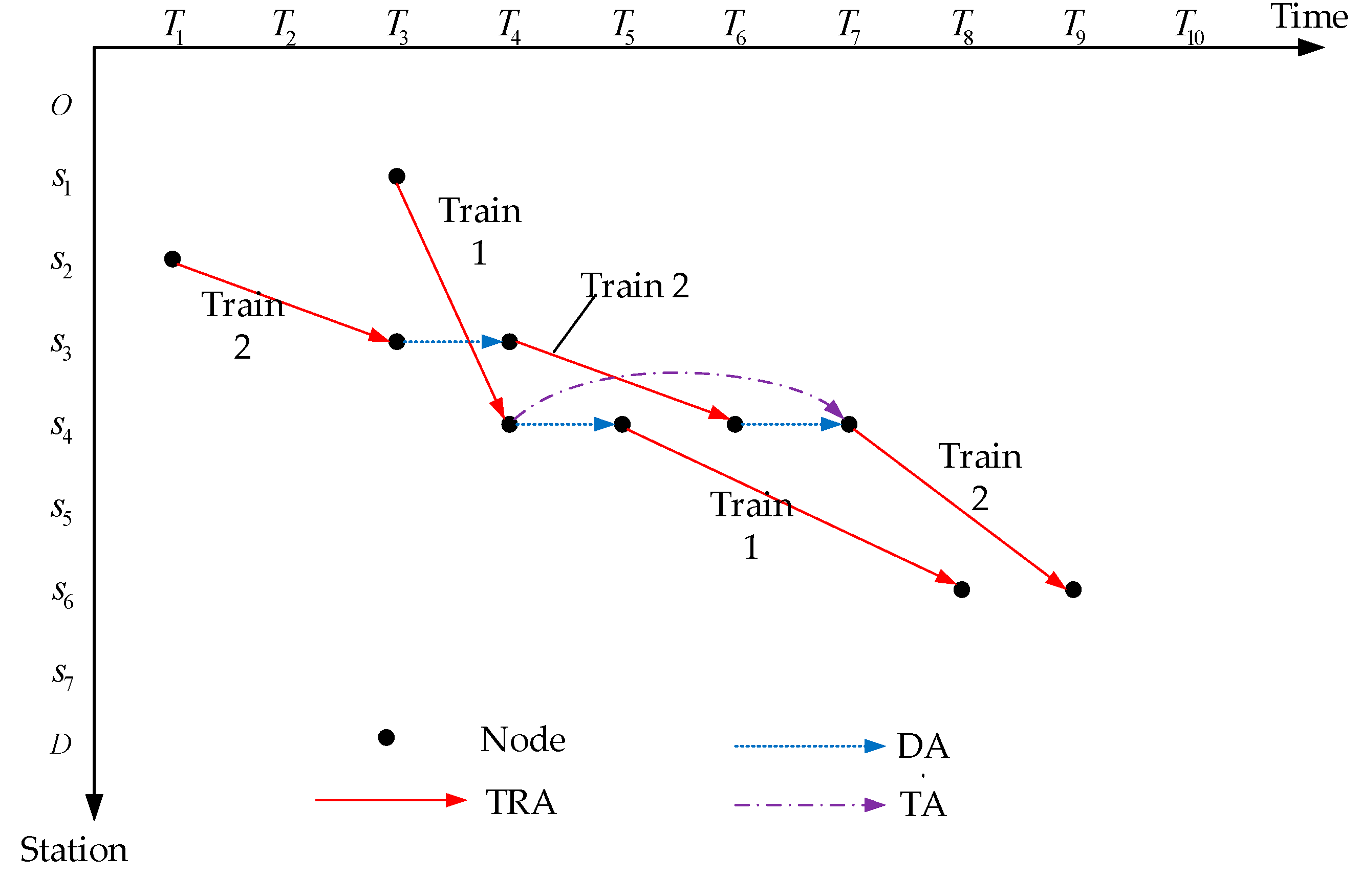
This paper refers to the RLPT service network in the literature [36,37,38,39,40,41,42,43,44,45,46,47,48,49]. As shown in Figure 1, for the vertical axis, $S_1$ to $S_7$ are RLPT handling stations. The horizontal axis represents time. The nodes in each row represent the same station at different times, and the nodes in each column represent different stations at the same time. When a car provides RLPT services, a series of arcs will be generated on the network. Figure 1 is a simple RLPT service network with two trains. The solid line is a train running arc (TRA), which represents the operation of passenger trains between RLPT handling stations. There are two types of horizontal dotted lines connected with nodes of the same RLPT handling station. The dotted line connecting the same trains from head to tail is a delayed arc (DA), which means that packages stay at the station waiting to be delivered. The dotted line connecting different trains from head to tail is a transit arc (TA), which means that packages are transferred from one train to another at the station. The main field definitions and data types of time– space nodes and arcs in the whole algorithm are shown in

Table 2. Field definitions of time–space network nodes.

Field	Definition	Data Type
node_id	ID index of time–space network node	Int
train_code	Train code on which node is located	String
station	Station corresponding to time–space node	Station class with attributes
time	Time corresponding to time–space node	Double

and

Table 3. Field definitions of time–space network arcs.

Field	Definition	Data Type
arc_id	ID index of time–space arc	Int
type	Type of time–space arc	Int
train_code	Train code on which time–space arc is located	String
start_node	Head node of time–space arc	Node with attributes
end_node	Tail node of time–space arc	Node with attributes
weight	Time difference between nodes at both ends of arc	Double

, and their ID indices start from 0. The indices of different time–space arcs are shown in

Table 4. Type index of different time–space arcs.

Time–space Arc	Type Index
TRA	0
DA	1
TA	2

.

Unlike the station-to-station transport process, when the two parts of door-to-station and station-to-door are included in the research scope, the constraints of transportation organization time and connection time need to be considered. When goods arrive at the sending or terminal station, the loading and unloading should be organized uniformly for a certain period of time, and the train’s stopping time should meet the loading and unloading operation time requirements of the goods. As shown in Figure 1, two trains can reach station $S_6$ close to destination $D$, but train 2’s departure time is too early, so the goods can only be sent to station $S_1$ at first, and then transported by train 1. In the process of transportation, the goods can be transferred to train 2 and transported to destination $D$ within time periods $T_4$ to $T_7$. Through a combination of a series of service arcs in the network, the process of RLPT is described, which can not only simulate the complex time constraints in the process of RLPT and properly calculate the K shortest path of OD, but also ensure timeliness in the process of transportation.

3.1.2. Principles and Restrictions of Path Search

For an OD pair with a given transport demand, the search for an RLPT path needs to satisfy the following restrictions following the organizational principles of RLPT, such as direct departure, reasonable division of transportation between long and short distances, and regional distribution:

• Time limit of loading and unloading operations. The loading and unloading of goods must be completed before the departure of the train; otherwise, the goods will not be able to undergo loading and unloading at the station.
• Minimum transit operating time limit. At the transfer station, the time interval between the arrival of the previous train and the departure of the next train is the transfer connection time. If the transfer connection time does not meet the limit of the shortest transfer operation time, the goods will not be able to undergo transit operation at the station.
• Limited number of transits. Each transit of goods will be accompanied by a loading and unloading operation, which not only consumes a lot of transportation resources, but also increases the uncertainty and reduces the safety of the transportation process. Therefore, it is stipulated that the maximum number of transits should be two, and any path with more than two transit times will be ignored.
• Transport timeliness constraint. The transportation time of the searched feasible path should not be too long, and the path should be guaranteed to meet the timeliness requirements of the cargo owner.

3.1.3. Preprocessing of Dynamic Time–Space Service Network before Path Search

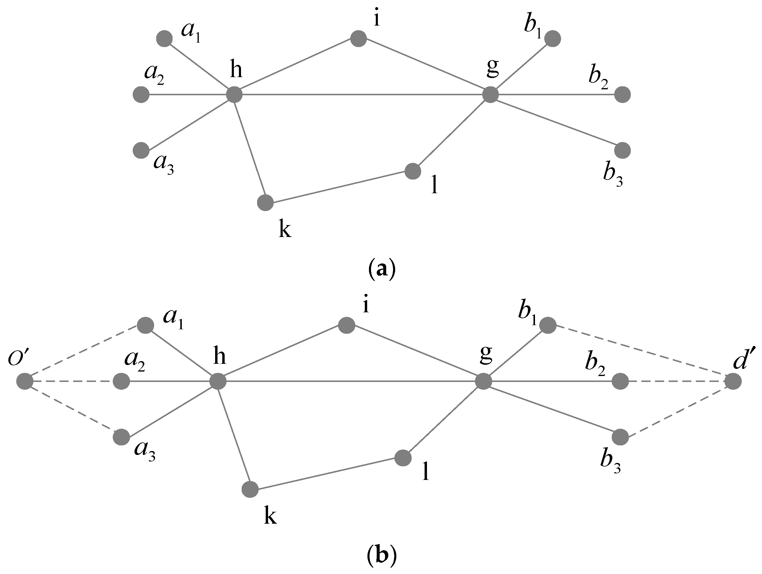
In the dynamic service network, there are many feasible paths between the start node and the end node of RLPT demand. The problem of the RLPT path is the problem of searching multiple feasible paths with greater timeliness and satisfying existing restrictions on the dynamic service network, which is essentially the K shortest path problem in the shortest paths. The dynamic time–space service network constructed by the method described in Section 3.1.1 has multiple start and end nodes. However, in graph theory, the path search can only be carried out in a graph with unique start and end nodes. If we search directly on the dynamic service network, we need to consider combinations of different start and end nodes, which will increase the complexity of the search process. A comparison between the initially constructed and processed dynamic time–space networks is shown in Figure 2. Figure 2a contains 11 network nodes, where $a_1,a_2,a_3$ and $b_1,b_2,b_3$ represent stations $a$ and $b$, respectively, at different times. When calculating the path of freight flow from station $a$ to station $b$, considering the time attributes of stations, there will be three start nodes and three end nodes in the network. The existing path search algorithms are not applicable to this network. As shown in Figure 2b, this problem can be solved by creating a virtual start arc (VSA) and virtual end arc (VEA) at both ends, with a unique virtual start node (VSN) and virtual end node (VEN). The dotted lines are virtual arcs at both ends, so that the whole network is a closed network with unique VSN and VEN. The specific operation methods are as follows: In the initial network, VSN $o^{\prime }$ and VEN $d^{\prime }$ with unique attribute identification are created. Since it is impossible to obtain the time when goods are delivered to the sending station, the time attribute of both can be set to 0. The attribute values of VSN and VSN are shown in

Table 5. Attribute values for virtual start node (VSN) and virtual end node (VEN).

Virtual Node	Node_Id	Train_Code	Station	Time
VSN	N (total number of network nodes) + 1	“0000”	VirtualStartStation	0
VEN	N (total number of network nodes) + 2	“0000”	VirtualEndStation	0

. We need to screen the network nodes that correspond to the sending station and consider the TRA that is passing through the particular station. If the train departure time corresponding to the node is later than the arrival time of the goods and the stop time of the train meets the loading operation time of the goods, then the node is connected with VSN $o^{\prime }$ to form a VSA. Similarly, the VEA connected with VEN $d^{\prime }$ can be constructed. The properties of virtual arcs at both ends are shown in

Table 6. Attribute values of virtual start arc (VSA) and virtual end arc (VEA).

Virtual Arc	Arc_Id	Type	Train_Code	Start_Node	End_Node	Weight
VSA	–1	3	“0000”	SN	$a_{1}or{a}_{2}or{a}_3$	0
VEA	–2	3	“0000”	$b_{1}or{b}_{2}or{b}_3$	VEN	0

. In path search, starting from $o^{\prime }$ and ending from $d^{\prime }$, we can search feasible paths for demand in dynamic time–space service networks with only start and end nodes. We set the arc weight of both virtual arcs to 0.

3.1.4. Feasible Path Set Generation Based on Improved A* Algorithm

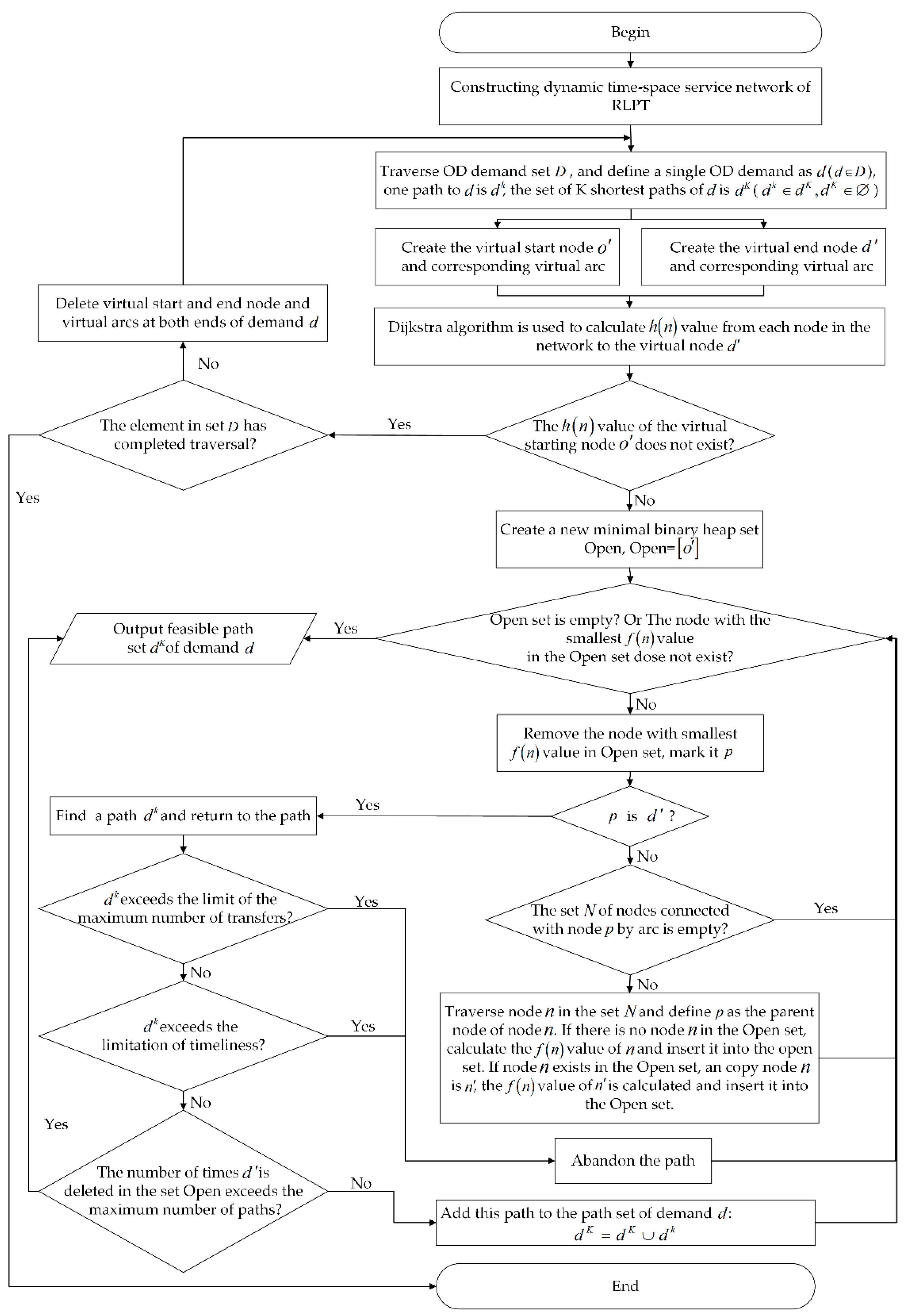
According to the structure of the dynamic time–space service network and the specific requirements of RLPT organizations, we can solve the K shortest path problem of RLPT by improving the A* algorithm. The existing K shortest path solving methods include double-sweep, A* algorithm, and deviation path algorithm [50,51]. The double-sweep algorithm has advantages in solving the path. However, obtaining path data requires reverse search, which is complex and difficult to understand [52]. In addition, compared with the double-sweep algorithm, the A* algorithm is easier to operate and has higher solution efficiency [53,54,55]. Therefore, the A* algorithm is used to solve the K shortest path in this study. The evaluation function of the A* algorithm is $f\left(n\right)=g\left(n\right)+h\left(n\right)$, where $g\left(n\right)$ is the actual cost from the initial node to the network node $n$ in the state space, and $h\left(n\right)$ is the estimated cost of the optimal path from network node $n$ to target node. The values of $g\left(n\right)$ and $h\left(n\right)$ will change with the change of A* algorithm execution time, but the shortest distance between two nodes is fixed and invariant, reflecting the property of local symmetry. The flowchart of the path search algorithm is shown in Figure 3, and the specific solving steps are as follows:

Step 1: Obtain basic dictionaries, such as passenger train schedule, station information, train information, demand set $D$, etc. Determine the basic parameters, such as minimum loading and unloading operation time and minimum transit operation time of each RLPT handling station, and maximum transit number of paths. According to the basic dictionary and basic parameters, construct the dynamic time–space service network of RLPT.

Step 2: Traverse OD demand set $D$, and define a single OD demand as $d$($d\in D$); one path to $d$ is $d^k$, and the set of K shortest paths of $d$ is $d^K$($d^k\in d^K,d^K\in \varnothing$).

Step 3: Determine whether the element in set $D$ has completed traversal. If the set traversal is complete, go to Step 13. Otherwise, according to the origin and destination information of demand $d$, create VSN $o^{\prime }$ and VEN $d^{\prime }$, then construct the virtual arcs at both ends based on the loading and unloading operation time requirements of each station and demand information to complete the network preprocessing of path search of demand $d$.

Step 4: Reverse arcs in service networks, take $d^{\prime }$ as the source node, use the Dijkstra algorithm to solve the shortest distance from $d^{\prime }$ to all nodes, that is, to find the $h\left(n\right)$ value of all nodes.

Step 5: Judge whether or not the $h\left(n\right)$ value of $o^{\prime }$ exists. If it does not exist, go to Step 2. Otherwise, go to Step 6.

Step 6: Create new minimum binary heap set Open (nodes in Open set are sorted by $f\left(n\right)$ value), insert $o^{\prime }$ into the Open set. The node in Open is the node through which the shortest path may pass.

Step 7: Determine whether the Open set is empty or the $h\left(n\right)$ value of the team head node of the Open set does not exist. If yes, output the feasible path set $d^K$ of demand $d$, go to Step 2. Otherwise, go to Step 8.

Step 8: Delete the node with the smallest $f\left(n\right)$ value in the Open set and mark it $p$. Determine if $p$ is $d^{\prime }$. If yes, find a path $d^k$ of demand $d$, return to the path, and go to Step 9. Otherwise, judge whether set $N$ of nodes connected with node $p$ by arc is empty. If yes, go to Step 7; otherwise, go to Step 12.

Step 9: Determine if $d^k$ exceeds the limitation of maximum transfer times. If yes, abandon $d^k$ and go to Step 7; otherwise, go to Step 10.

Step 10: Judge whether $d^k$ exceeds the limitation of timeliness. If yes, abandon $d^k$ and go to Step 7; otherwise, go to Step 11.

Step 11: Determine whether the number of $d^{\prime }$ deleted in the set Open exceeds the maximum number of paths. If yes, output the feasible path set $d^K$ of demand $d$, and go to Step 2. Otherwise, $d^K=d^K\cup d^k$ and go to Step 7.

Step 12: Traverse node $n$ in set $N$ and define $p$ as the parent node of node $n$. If there is no node $n$ in the Open set, calculate the $f\left(n\right)$ value of $n$ and insert it into the Open set. If node $n$ exists in the Open set and copy node $n$ is $n^{\prime }$, calculate the $f\left(n\right)$ value of $n^{\prime }$ and insert it into the Open set. Go to Step 7.

Step 13: When the traversal of demand set $D$ is completed, feasible paths of all demands have been found and the algorithm ends.

Through the path search algorithm mentioned above, the path set of all demands can be generated. Our proposed RLPTS formulation model is based on the feasible path set of demand, avoiding the allocation of goods flow on the infeasible path. The model aims to maximize the revenue of transportation enterprises and concentrates on the situation where the transportation demand cannot be satisfied due to the limited path capacity and insufficient luggage vehicle capacity. By solving the model, the flow allocated on each path can be obtained.

3.2. Flow Distribution Model Based on Feasible Path

3.2.1. Assumptions and Parameter Descriptions

Specifically, the decision variables are set up to provide convenience in obtaining the distribution scheme of cargo flows. The decision variables count the transport volume of goods assigned to each path. In this manner, the distribution scheme of cargo flows is obtained.

Without the loss of generality, this study further makes the following assumptions:

• Theoretically, the loading capacity of the train is limited by its own capacity, volume, and weight of goods. To simplify the solution, only the effect of weight on the train’s loading capacity is considered in the model.
• Without considering the restriction of mixed cargo loading, we studied the formulation of RLPTS from the perspective of system optimization.
• Assuming that RLPT handling station has no limitation on capacity, it can meet the requirements of large quantities of stacked goods.

Regardless of the specific composition of each demand, we consider demand as objects that can be split arbitrarily by weight and transported by multiple transportation paths.

The parameter and decision variable definitions of the model are as follows:

Parameter	Description
$D$	OD set of cargo flows, $d\in D$
$A$	Set of service arcs, $a\in A$
$d^k$	kth ($k=1,2\cdot \cdot \cdot$) path of demand $d$
$d^K$	Set of K shortest paths of demand $d$, $d^k\in d^K$
${\omega }_{d^k}$	Cost of demand $d$ transported by path $d^k$, yuan/kg
$x_d$	Demand $d$ for volume be transported through path $d^k$
$r_d$	Freight of demand $d$, yuan/t
$x_{d^k}$	Demand $d$ for volume to be transported through path $d^k$
$\tau$	Cost per kilogram of cargo loaded and unloaded, yuan/kg
$\rho$	Penalty charges for unmet demands, yuan/kg
${\gamma }_a^{d^k}$	If arc $a$ is selected by path $d^k$, the value is 1; otherwise, 0
$c_a$	Transportation capacity of arc $a$
$c_{d^k}$	Transportation capacity of path $d^k$

3.2.2. Objection Function

The model focuses on the objective function of maximum total profit of the transportation enterprise in order to meet customers’ demand to the greatest extent. Total profit is the difference between total revenue and total cost. Total revenue comes from completing the transport of goods. Total cost mainly includes transportation and time costs. The time cost of goods describes the timeliness of door-to-door transport. The lower the timeliness, the higher the time cost. Therefore, a model with maximum total profit can ensure priority distribution of goods to the path with high timeliness and ensure the timeliness of door-to-door transportation. The model objective function is as follows:

$$Maxz={\displaystyle \sum _{d\in D}{\displaystyle \sum _{d^k\in d^K}\left[x_{d^k}\cdot \left(r_d-{\omega }_{d^k}-2\tau \right)\right]}-{\displaystyle \sum _{d\in D}\left(x_d-{\displaystyle \sum _{d^k\in d^K}{x}_{d^k}}\right)\cdot \rho }}$$

(1)

3.2.3. Constraint Conditions

RLPTS is mainly influenced by railway passenger train transport schemes. It is also affected by the total demand of luggage and packages, the loading capacity of luggage vehicles, and the transport capacity of the path. The specific constraints are as follows:

The transport capacity of each path in the RLPT service network is limited, and the demand may require multiple paths to transport. Moreover, due to capacity constraints, some of the demand may not be transported. Therefore, the flow volume of demand to be transported is less than or equal to the total demand:

$${\displaystyle \sum _{d^k\in d^K}{x}_{d^k}\le x_d}\hspace{1em}\hspace{1em}\forall d\in D,d^k\in d^K$$

(2)

The maximum loading capacity of a train is the sum of the loading capacity of all luggage and package vehicles on the train. Because the train can be loaded and unloaded at each stop station, it can carry goods in different sections. Therefore, the total demand for goods transported in the same section should not exceed the maximum loading capacity of the vehicle. That is to say, any TRA in the service network must comply with the following formula:

$${\displaystyle \sum _{d\in D}{\displaystyle \sum _{d^k\in d^K}\left(x_{d^k}\cdot {\gamma }_a^{d^k}\right)}}\le c_{a\hspace{1em}\hspace{1em}}\forall a\in A$$

(3)

The meaning of the decision variable is the traffic volume allocated to each path, with the minimum being 0 and the maximum not exceeding the transport capacity of the path, namely,

$$0\le x_{d^k}\le c_{d^k}\hspace{1em}\hspace{1em}\forall d\in D,d^k\in d^K$$

(4)

3.2.4. Evaluation Indices

The result of traffic volume allocation is the traffic volume allocated on each feasible path and can be evaluated by the following indicators:

● Average transit times (ATT)

In this paper, the average transit time of demand is used to describe the transit times of a demand. If demand $d$ is transported by $n$ feasible paths, the completed traffic volume is $d_{total}$ ($d_{total}\le x_d$), the traffic volume on each path is $d_1,d_2,d_3,\dots ,d_n$, and the transit time of each path is $m_1,m_2,m_3,\dots ,m_n$. The ATT $d_{average}$ of demand $d$ is

$$d_{average}={\displaystyle \sum _{i=1}^n{m}_i\frac{d_i}{d_{total}}}$$

(5)

If the RLPT service network completes the transportation of $n$ demand, the ATT $D_{average}$ of all demands in the transportation is

$$D_{average}={\displaystyle \sum _{i=1}^n\frac{d_{average}^n}{n}}$$

(6)

The closer ATT is to 0, the more the goods tend to be transported by direct mode, which indicates that the flow distribution is better.

● Train capacity utilization ratio (TCUR)

The TCUR reflects the utilization situation of passenger train luggage vehicle capacity. Using statistics of the utilization ratio of train capacity is beneficial to analyze the bottleneck of restricting RLPT. Supposing the train passes through sections $s_1,s_2,s_3,\dots ,s_n$ in sequence, the distance of each section is $l_1,l_2,l_3,\dots ,l_n$, the goods loaded on each section is $k_1,k_2,k_3,\dots ,k_n$, and the carrying capacity of the train is $c_{train}$, then the formula for calculating the TCUR is as follows:

$$u_{train}={\displaystyle \sum _{j=1}^n\frac{l_j\cdot k_j}{c_{train}\cdot {\displaystyle \sum _{i=1}^n{l}_i}}}$$

(7)

● Transfer volume of transfer station

The daily transit volume completed by the transit station reflects the daily transit operation of the station. Assume that the paths pass through transfer station $T$ with ${\lambda }^1,{\lambda }^2,{\lambda }^3,\dots ,{\lambda }^n$, the traffic volume on each path is ${\lambda }_1,{\lambda }_2,{\lambda }_3,\dots ,{\lambda }_n$. Then the transfer volume $T_{\lambda }$ of transfer station $T$ is

$$T_{\lambda }={\displaystyle \sum _{i=1}^n{\lambda }_i}$$

(8)

If the result produced by flow distribution is more in line with the actual transfer volume undertaken by the transfer station, it indicates that the flow distribution is working well.

4. Empirical Studies

Visual Studio 2019 software (C#) was used to design the search path algorithm and Cplex solver (C# programming language) was used to solve the flow distribution model. It is a linear programming model that is efficient for use in a dynamic time–space service network of any size. Concretely, the traffic assignment of cargo flows is a combinatorial optimization problem. Given that the problem includes trains and demand, its scale is related to the quantity of demand (denoted by d), the number of trains (denoted by t), and the maximum value of k. The problem has in general (d^k) variables and (d + t + d^k) constraints, and the global optimal solution was obtained within 180 min in this study (path search took 165 min and model solving took 15 min).

4.1. Related Parameter Values

The model and algorithm were verified with the actual operation data of RLPT and the train schedule was provided by CRE in March 2018. There are 12,471 daily OD demands, 415 RLPT handling stations, and 130 transfer stations, while 1880 passenger trains are equipped with luggage wagons. Based on train schedules and station information, a dynamic time–space service network of RLPT with 44,122 time–space nodes and 399,548 time–space arcs was constructed.

4.1.1. Parameter Values in Path Search Algorithm

The actual operation data of CRE in 2018 were used to set various parameters in the algorithm. Assuming that loading and unloading conditions at each station are the same, minimum loading and unloading operation time is 2 min, minimum transit operation time is 5 h, and loading and unloading capacity and transit capacity of goods are both 300 kg/min. One luggage vehicle is arranged in each passenger train group. The carrying capacity of the vehicle is 12 t which considers that small goods will be tossed around lightly. Path search is carried out based on train running time as weight, in order to limit the search breadth and depth of the algorithm; it is necessary to find up to 10 feasible paths for each demand, and each path has a maximum of two transfers.

4.1.2. Freight Rates and Costs in the Model

1. Transport price $r_d$ for every OD

According to the actual operation data of CRE in 2018, the start station code, end station code, batch, number, weight, unit transport price, and time limit of different demands are shown in

Table 7. Start station code, end station code, batch, number, weight, time limit, and unit transport price ($r_d$) of different demands.

Start Station Code	End Station Code	Batch	Number	Weight (kg)	Unit Transport Price (kg/yuan)	Time Limit (day)
0902	0102	5	6	21	2.19	2
0904	1201	1	3	21	5.20	1
1203	3226	3	3	21	2.81	3
1001	3341	2	1	21	2.63	2
4719	3348	4	1	21	0.98	2
0901	9887	25	772	10,480	3.69	2
1201	9887	28	1588	18,699	1.57	2

(data on partial transportation demands).

2. Transport cost ${\omega }_{d^k}$ and loading or unloading operation cost $\tau$ of every path $d^k$

According to the Freight Rates Management Department of the China Railway General Corporation, the loading or unloading operation cost $\tau$ (yuan/kg) is 2, the transport cost ${\omega }_{d^k}$ of the path includes a locomotive traction fee ${\varphi }_{d^k}$, transfer operation fee ${\psi }_{d^k}$, and transportation time cost ${\mathsf{\Omega }}_{d^k}$, as follows:

● Locomotive traction fee ${\varphi }_{d^k}$

This is the cost incurred by the locomotive acting as the carrier of luggage for the traction train. The cost of locomotive traction for one kilometer per kilogram of luggage is called the unit locomotive traction fee, which is yuan/(kg*km). We define $f_a$ as the unit locomotive traction fee when the locomotive acts as arc a, and if $l_a$ is the distance of arc a, then the locomotive traction fee of path $d^k$ can be expressed as

$${\varphi }_{d^k}={\displaystyle \sum _{a\in d^k}{f}_a\cdot l_a}$$

(9)

● Transfer operation fee ${\psi }_{d^k}$

This is the cost incurred by the transfer operation. The transfer operation fee of demand is defined as the cost incurred by one transfer operation per kilogram of goods, in yuan/kg. The transit operation fee of path $d^k$ is related to the number of transit operations and the unit transit operation fee of goods. We define $\mu$ and ${\theta }_{d^k}$ as the unit transit cost of goods and the number of transit times of route b, respectively. Then the transfer operation fee of path $d^k$ can be expressed as

$${\psi }_{d^k}=\mu \cdot {\theta }_{d^k}$$

(10)

● Transportation time cost ${\mathsf{\Omega }}_{d^k}$

Assuming that the transportation time of path $d^k$ is $T_{d^k}$, we define V as the time cost calculation coefficient, in yuan/(min*kg). The transportation time cost ${\mathsf{\Omega }}_{d^k}$ of path $d^k$ is

$${\mathsf{\Omega }}_{d^k}=V\cdot T_{d^k}$$

(11)

Then the formula for calculating the cost of path $d^k$ is as follows:

$${\omega }_{d^k}={\varphi }_{d^k}+{\psi }_{d^k}+{\mathsf{\Omega }}_{d^k}={\displaystyle \sum _{a\in d^k}{f}_a\cdot l_a}+\mu \cdot {\theta }_{d^k}+V\cdot T_{d^k}$$

(12)

According to the actual operation data of CRE in 2018, the average locomotive traction fee $f_a$, the average unit transit cost $\mu$, and the time cost calculation coefficient V were determined to be 0.05, 0.5, and 0.004, respectively.

3. Penalty charges $\rho$ for unmet demands

Customers hope their goods will arrive at the station within the specified time range (time limit: $T_{arrive}$/min). When the transportation time ($T_s$/min) exceeds the expected arrival time, it can be considered that this OD demand has not been met, and the railway department must reduce the transportation cost to some extent. We define ${\xi }_d$ and $\rho$ as penalty coefficient of unit goods exceeding expected arrival time and penalty cost per unit goods (yuan/ton), respectively; then the required time penalty cost can be expressed as

$$\rho =\{\begin{array}{ll}0& \left(T_s-T_{arrive}\right)\ge 0\\ {\xi }_d\left|T_s-T_{arrive}\right|& \left(T_s-T_{arrive}\right)<0\end{array}$$

(13)

Based on research of the penalty coefficient of RLPT by Zheng (2012), the average penalty coefficient ${\xi }_d$ is determined to be 1.2.

4.2. Results and Discussion

Under the dynamic time–space service network, the total number of demand paths that can be solved by the A* algorithm is 117,227. The RLPTS of partial demands, transfer volume of transfer stations and train capacity utilization ratio are shown in

Table 8. The RLPTS of partial demands.

Demand ID	Start Station Name	End Station Name	RLPTS
1	Changsha	Qiqihaer	(Changsha, 00T124A7,ShenyangBei)(ShenyangBei,0K1082A4,Qiqihaer *)
1	Changsha	Qiqihaer	(Changsha,00T124A8,ShenyangBei)(ShenyangBei,0K1082A4,Qiqihaer *)
1	Changsha	Qiqihaer	(Changsha,00T124A7,ShenyangBei)(ShenyangBei,0K1082A5,Qiqihaer *)
1	Changsha	Qiqihaer	(Changsha,00T124A8,Zhangchun *)(Zhangchun,0K1082A5,Qiqihaer *)
1	Changsha	Qiqihaer	(Changsha,000T14A5,ShenyangBei *)(ShenyangBei,0K1082A4,Qiqihaer *)
1	Changsha	Qiqihaer	(Changsha,00T254A0,Tianjin *)(Tianjin,0K1082A4,Qiqihaer *)
1	Changsha	Qiqihaer	(Changsha,000T14A5,ShenyangBei *)(ShenyangBei,0K1082A5,Qiqihaer *)
1	Changsha	Qiqihaer	(Changsha,00T254A0,Tianjin *)(Tianjin,0K1082A5,Qiqihaer *)
1	Changsha	Qiqihaer	(Changsha,000Z14A0,ShenyangBei *)(ShenyangBei,0K1082A4,Qiqihaer *)
1	Changsha	Qiqihaer	(Changsha,000Z14A0,ShenyangBei *)(ShenyangBei,0K1082A5,Qiqihaer *)
2	Botou	Qiqihaer	(Botou,0K1450A2,ShenyangBei)(ShenyangBei,00K546A3,Qiqihaer *)
2	Botou	Qiqihaer	(Botou,0K1450A1,Tianjin)(Tianjin,00K546A3,Qiqihaer *)
2	Botou	Qiqihaer	(Botou,00K956A2,Tianjin)(Tianjin,00K546A3,Qiqihaer *)
2	Botou	Qiqihaer	(Botou,001450A0,Tianjin)(Tianjin,00K546A3,Qiqihaer *)
2	Botou	Qiqihaer	(Botou,001450A0, Zhangchun)(Zhangchun,0K1082A4,Qiqihaer *)
2	Botou	Qiqihaer	(Botou,001450A0, Zhangchun)(Zhangchun,0K1082A5,Qiqihaer *)
2	Botou	Qiqihaer	(Botou,00K956A3,Tianjin)(Tianjin,0K1082A4,Qiqihaer *)
2	Botou	Qiqihaer	(Botou,0K1450A1,Tianjin)(Tianjin,0K1082A4,Qiqihaer *)
2	Botou	Qiqihaer	(Botou,00K956A2,Tianjin)(Tianjin,0K1082A5,Qiqihaer *)
2	Botou	Qiqihaer	(Botou,00K956A3,Tianjin)(Tianjin,0K1082A5,Qiqihaer *)

Notes: * represent that the station is departure station or end station of the train.

,

Table 9. Transfer volume of transfer stations.

Station Name	Transit Volume (kg)
Haerbinxi	860
Qiqihaer	3097
Zhangchun	28,214
Shenyangbei	20,662
Shenyang	14,015
Jilin	3424
Jinzhou	31,063
Beijingxi	1270
Beijing	6412
Tianjin	47,654
Shijiazhuang	23,874

and

Table 10. Train capacity utilization ratio.

Train Code	Utilization Rate (%)
0000K5A0	0.11
0000T1A0	0.01
0000T2A0	0.04
0000T7A0	0.03
0000T8A0	0.12
0000T9A2	0.05
0000Z1A0	0.04
0000Z2A0	0.27
0000Z3A0	0.66
0000Z3A1	0.53

, respectively. (Table 8, Table 9 and Table 10 in the Supplementary Materials are the complete data calculated.)

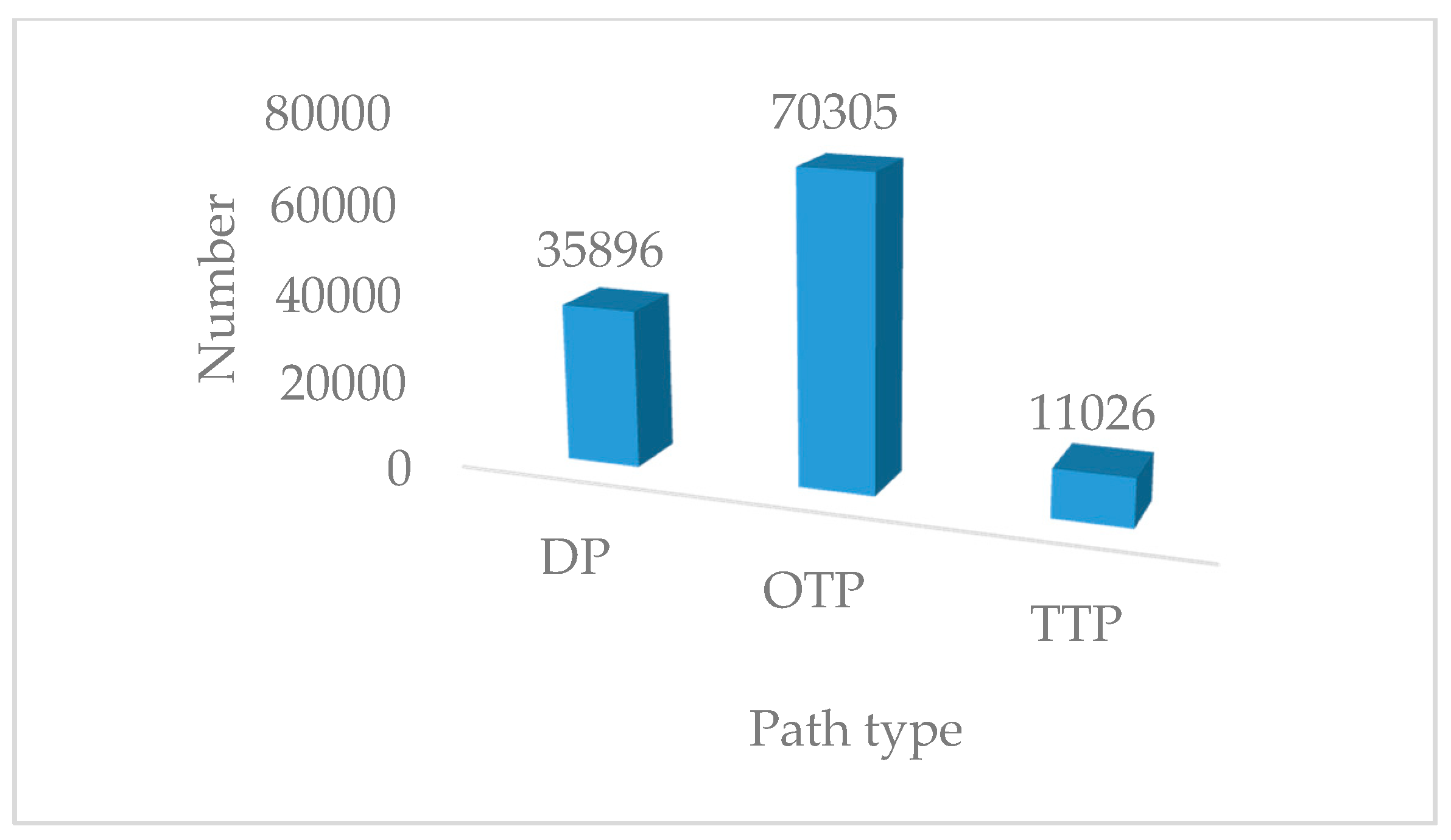
The numbers of direct paths (DPs), one transit paths (OTPs), and two transit paths (TTPs) are shown in Figure 4.

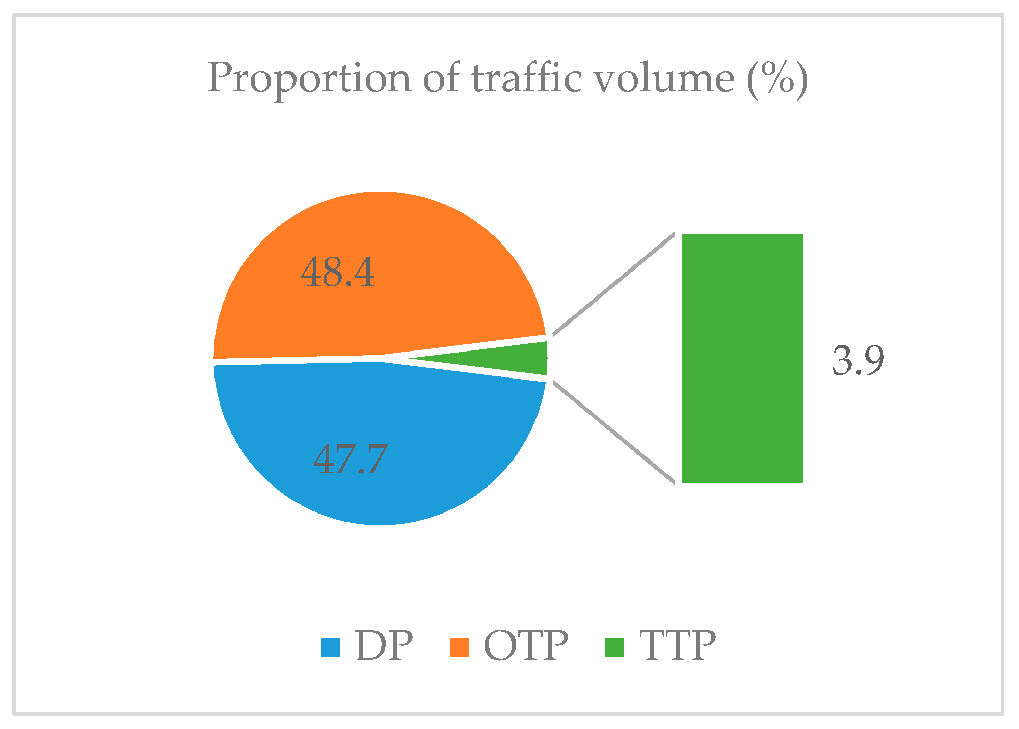
The ATT calculated by the model is 0.608; the closer ATT is to 0, the more the goods tend to be transported by direct mode, indicating that the result of flow distribution is better. Compared with the values of 1.029 and 2 of Zu (2009) and Zheng (2012), it is greatly improved. The proportions of traffic volume through DP, OTP, and TTP are shown in Figure 5. It indicates that most of the demands can be completed through the generated DP and OTP, which realizes well the basic principles of RLPT organization with less transit as far as possible, and the validity of the model is proved.

The results show that 97.6% of the transportation demand is completed, which can basically meet the current RLPT demand. Unshipped demand is concentrated in Xuzhou, Guiyang, Tianjin, Lanzhou, Beijing West, and other stations, mainly because the demand for transportation or transition at these stations is high, and the capacity of trains passing through the stations is insufficient, which is basically in line with the actual situation.

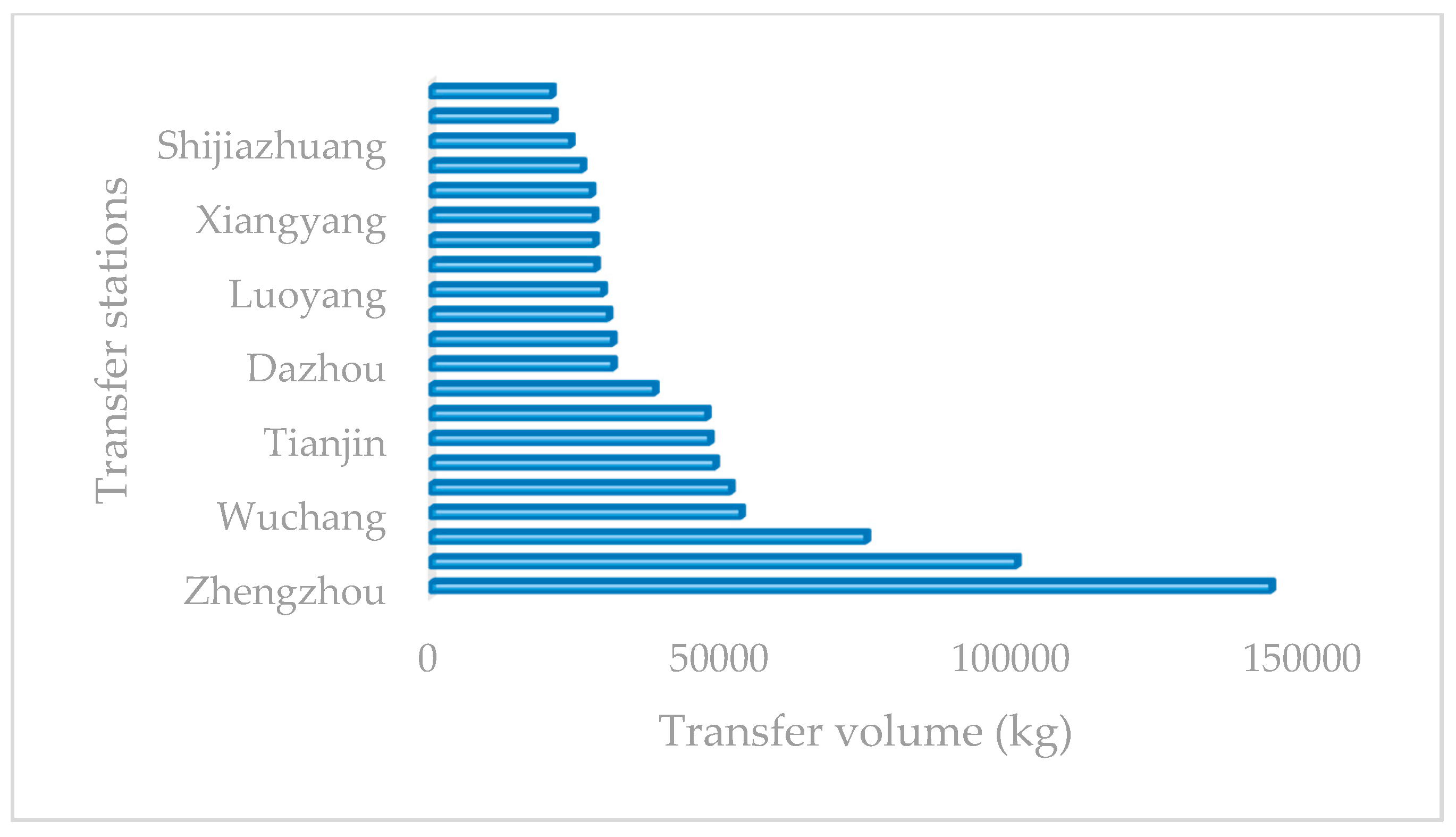
The transfer capacity of some transfer stations is shown in Figure 6. Zhengzhou, Xuzhou, Xi ‘an, Wuchang, and other stations have undertaken a large number of transfer operations, which is due to an excessive number of transit trains passing through these stations.

A total of 1880 trains is involved in RLPT, and the numbers of trains with different TCURs is shown in Figure 7. Overall, TCUR is still considered to be at a low level. It shows that the railway department has provided sufficient transport capacity for RLPT to meet the current market demand.

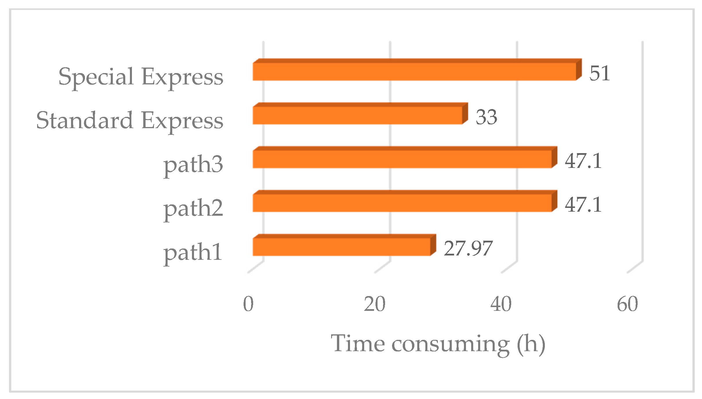
Take Harbin West–Shanghai, with a demand volume of 3409 kg, as an example to verify and illustrate the two-stage RLPTS formulation method proposed in this paper. Referring to the actual operation data of CR-SF, the average delivery time for S.F. Express in the same city is 2 h. Considering that the delivery time of goods to consignees should not be too late, it is stipulated that goods arriving after 21:00 will be postponed to the next day, and the delivery time will start at 08:00 every day. The flow distribution results are shown in

Table 11. Harbin West–Shanghai traffic volume distribution results.

Path	Sent Time	Train Code	Transfer Station	Arrival Time	Customer Receipt Time	Door-to-Door Timeliness	Volume (kg)
1	00:51	Z174	—	00:49 (2nd day)	14:49 (2nd day)	27 h, 58 min	3409
2	00:51	Z174 K292	Suzhou	05:34 (3rd day)	10:00 (3rd day)	47 h, 6 min	0
3	00:51	Z174 K378	Suzhou	05:24 (3rd day)	10:00 (3rd day)	47 h, 6 min	0

. As can be seen, the timeliness of path 1 is the highest; in the case of meeting capacity, the flow distribution model considering time cost will give flow distribution priority to path 1 with higher timeliness, which can avoid flow allocation issues on the unfeasible path and verifies the validity of the model.

The timeliness comparison of paths calculated by the model and algorithm and related products of S.F. Express are shown in Figure 8. It can be seen that the transportation timeliness of path 1 undertaking flow is better than that of S.F. Express, which verifies the accuracy of the model and algorithm.

4.3. Result Comparison

This paper further verifies the algorithm’s superiority and takes the RLPTS of “Beijing–Guangzhou” as an example to compare the RLPTS generated here with the RLPTS currently used by CRE. The contrast of the two plans is shown in

Table 12. Contrast of two RLPTS.

RLPTS in This Paper				RLPTS Currently Used
Train Number	Transfer Station	Cost (yuan)	Time (min)	Train Number	Transfer Station	Cost (yuan)	Time (min)
Z12	–	3281.06	1313	T15	–	3210.06	1326
T12	–	2659.87	1320	T29	–	2541.27	1348
2251, K93	Chengde	2226.74	1724	T1, K93	Changsha	2353.09	1885
K48, Z12	Tianjin	977.46	1933	K17, T25	Zhengzhou	1401.73	2013

.

As seen by the contrast in Table 12, the RLPTS generated in this paper gives two through paths and two paths with one transfer. The transfer frequency of this plan equals that of the RLPTS currently used, but with less time consumption and lower general cost. Therefore, the RLPTS in this paper is feasible, and better than the RLPTS currently used from the perspective of time and cost.

5. Conclusions

In this paper, we analyzed the characteristics of RLPT demand and defined the guiding ideology of RLPTS formulation with timeliness as the core. Based on its characteristics, we gave a formulation idea of a two-stage method of RLPTS. That is, we decomposed the RLPTS formulation problem into subproblems, one of which was the construction of a dynamic time–space service network based on passenger train schedules and demand information. Then, based on the time–space network, an improved A* algorithm was used to search feasible paths of RLPT. The other subproblem involved building a flow distribution model by considering the constraints of path capacity, capacity of luggage vehicles, and transport timeliness. The main innovation points of the algorithm and model proposed in this paper were as follows: (1) based on passenger schedules and demand information, we constructed a dynamic time–space service network of RLPT; (2) the initial constructed time–space network was processed into a closed time–space network at both ends, and the A* algorithm adapted to the network was adopted to generate a feasible path set of all transportation demands; and (3) considering the relevant important constraints, a flow distribution model was constructed. According to the solution results of the model, ATT, TCUR, and the transfer volume of transfer station were calculated. In the end, the RLPTS for all transportation demands was obtained, and the current resource utilization situation and development bottleneck of RLPT were analyzed.

The numerical studies demonstrated the following: (1) the ATT of feasible paths calculated by our proposed algorithm was close to 0, which is in line with the basic principle of minimizing transit for RLPT, that is, demand tends to be transported by direct paths; and (2) the RLPTS solved by the model can basically meet the current demand. In addition, it can be seen from the calculated TCUR and transit volume of transfer stations that the current RLPT capacity is larger than current demand for transportation, and some transfer stations have large cargo flow pressure, which can be improved through construction of related infrastructure.

Compared with the problems that exist in the current RLPTS formulation method, we demonstrated ways to resolve the issues with a two-stage method, which can reduce the difficulty of solving the problem and improve the efficiency of the scheme formulation. At the same time, the two-stage method can adapt to any dynamic changes in demand, ensure the timeliness of transportation, avoid the allocation of flow on unfeasible paths, and also consider the formulation of schemes from the perspective of global optimization, which is suitable for solving large-scale time–space network problems. Last but not least, the numerical studies demonstrate that this method can accomplish the entire road with the help of RLPTS within a short period of time and verifies the feasibility and effectiveness of the model and algorithm.

Although the model and algorithm proposed in this paper are highly efficient under certain assumptions, they do not consider the impact of the volume of goods, which to some extent leads to the limitation of problem solving. Future research will consider the volume and weight of cargo comprehensively and optimize the model and algorithm from the perspective of practical application.

References

1. Armstrong & Associates, Inc. Global and Regional Infrastructure, Logistics Costs, and Third-Party Logistics Market Trends and Analysis; Armstrong & Associates, Inc.: Milwaukee, WI, USA, 2016. [Google Scholar]
2. Cao, L.H. Research on Package Pathway Selection Problem with Capacity Constrains in Time-Varying Network. Ph.D. Thesis, Beijing Jiaotong University, Beijing, China, 2007. [Google Scholar]
3. Li, X.-J. Research on Railway Package Transport Organization and Optimization. Ph.D. Thesis, Beijing Jiaotong University, Beijing, China, 2006. [Google Scholar]
4. Shen, R. Research on Service Network Design Theory and Method of Railway Package Transport. Ph.D. Thesis, Beijing Jiaotong University, Beijing, China, 2006. [Google Scholar]
5. He, Z.H. Thought on organization method of passenger package transportation of passenger dedicated lines. Railw. Transp. Econ. 2006, 28, 65–66. [Google Scholar]
6. Huang, Z. Research on the transport system of dedicated passenger transport lines. Railw. Purch. Logist. J. 2007, 2, 21–22. [Google Scholar]
7. Xu, C.C. Research on the application of railway luggage and package train. J. Beijing Jiaotong Univ. 2008, 5, 104–106. [Google Scholar]
8. Zu, Y.; Li, Y.Q. Research on the development of railway express freight transport. China Storage Transp. 2019, 7, 91–93. [Google Scholar]
9. Wang, G.D. Research on organization method and optimization of railway luggage and package transportation. Technol. Enterp. 2012, 16, 88. [Google Scholar]
10. Feng, S.R. Marketing strategy analysis of railway luggage and package transportation market. Railw. Econ. Res. 2015, 5, 39–41. [Google Scholar]
11. Chen, J.L. Reflections on the development of railway express service in China. China Transp. Rev. 2006, 2, 71–74. [Google Scholar]
12. Chen, J.L. Innovation of railway part load freight service system to meet market demand. Railw. Freight Transp. 2006, 7, 1–3. [Google Scholar]
13. Ji, C.X.; Liu, J. Research on Marketing Strategy of Railway Luggage and package transportation. J. Beijing Jiaotong Univ. 2000, 24, 100–105. [Google Scholar]
14. Li, H. A preliminary study on the development of railway express transportation market. Railw. Transp. Econ. 2006, 28, 46–47. [Google Scholar]
15. Yi, C.Z.; Zhong, Y. Problems in railway baggage transportation and promotion stragegies. J. Beijing Jiaotong Univ. 2001, 25, 98–100. [Google Scholar]
16. Zhang, G.P. Marketing strategy of railway luggage and package express. Transp. Econ. 2005, 27, 66–68. [Google Scholar]
17. Huang, P.; Zhang, Z.Y. Research on model and algorithms of transportation network traffic allocation problem. Chin. J. Manag. Sci. 1999, 7, 48–54. [Google Scholar]
18. Yan, H.X.; Liang, D.; Zhang, T.W. Optimal model of railway network distribution. J. Xinan Jiaotong Univ. 2007, 42, 758–762. [Google Scholar]
19. Liu, C.; Lin, B.L.; Wang, J.X.; Liu, S.; Wu, J.; Li, J. Flow assignment model for quantitative analysis of diverting bulk freight from road to railway. PLoS ONE 2017, 12, e0182179. [Google Scholar] [CrossRef] [PubMed]
20. Wang, Y.; Liu, J. Study on the method of optimizing the schemes of railway luggage and package express special train. J. Transp. Syst. Eng. Inf. Technol. 2007, 7, 125–129. [Google Scholar]
21. Lin, B.L.; Wang, Z.M.; Ji, L.J.; Tian, Y.M.; Zhou, G.Q. Optimizing the freight train connection service network of a large-scale rail system. Transp. Res. B Meth. 2012, 46, 649–667. [Google Scholar] [CrossRef]
22. Zhu, E.; Cranic, T.G.; Gendreau, M. Scheduled Service Network Design for Freight Rail Transportation. Oper. Res. 2014, 62, 383–400. [Google Scholar] [CrossRef]
23. Newton, H.N.; Barnhart, C.; Vance, P.H. Constructing railroad blocking plans to minimize handling costs. Transport. Sci. 1998, 32, 330–345. [Google Scholar] [CrossRef]
24. Barnhart, C.; Jin, H.; Vance, P. Railroad blocking: A network design application. Oper. Res. 2000, 48, 603–614. [Google Scholar] [CrossRef]
25. Bai, R.; Wallace, S.W.; Li, J.; Chong, A.Y.L. Stochastic service network design with rerouting. Transp. Res. B Meth. 2014, 60, 50–65. [Google Scholar] [CrossRef]
26. Dong, X.Y.; Liu, J.; Ji, C.X. Design and research on network model of express freight transport based on multiple transport modes. Logist. Technol. 2006, 10, 36–39. [Google Scholar]
27. Ji, S.F.; Luo, R.J. A hybrid estimation of distribution algorithm for multi-objective multi-sourcing intermodal transportation network design problem considering carbon emissions. Sustainability 2017, 9, 1133. [Google Scholar]
28. Di, X.; Ma, R.; Liu, H.X.; Ban, X.G. A link-node reformulation of ridesharing user equilibrium with network design. Transp. Res. B Meth. 2018, 112, 230–255. [Google Scholar] [CrossRef]
29. Zu, Y.; Tian, N.; Yang, D.Y. Route algorithms for railway luggage and package transportation. China Railw. Sci. 2008, 29, 111–115. [Google Scholar]
30. Zu, Y.; Tian, N.; Yang, D.Y. Study on the programming model of railway luggage transportation. J. China Railw. Soc. 2009, 31, 20–24. [Google Scholar]
31. Chen, J.L. Study on compiling method of railway packaging and transportation schemes. China Railw. Sci. 2012, 1, 108–112. [Google Scholar]
32. Liu, J.T.; Zhou, X.S. Capacitated transit service network design with boundedly rational agents. Transp. Res. B Meth. 2016, 93, 225–250. [Google Scholar] [CrossRef] [Green Version]
33. Liu, Y.; Zu, X.N.; Yan, B.C. Optimization of high-speed railway luggage transportation scheme based on existing operating diagram. J. Wuhan Univ. Technol. Transp. Sci. Eng. 2016, 40, 1038–1042. [Google Scholar]
34. Liu, X.W. Study on Time Reliability of Railway Baggage Train. Master’s Thesis, Xinan Jiaotong University, Chengdu, China, 2016. [Google Scholar]
35. Yang, J.H.; Liu, L.Z.; Li, X.J. Study on optimizing the fast transport of scattered goods by railway luggage trains. J. Railw. Sci. Eng. 2016, 13, 1426–1432. [Google Scholar]
36. Lin, B.L. A study of car-to-train assignment problem for rail express cargos on scheduled and unscheduled train service network. arXiv 2018, arXiv:1803.05760v1. [Google Scholar] [CrossRef] [PubMed]
37. Lin, B.L.; Liu, C.; Wang, J.X.; Liu, S.Q.; Wu, J.P.; Li, J. Modeling the railway network design problem: A novel approach to considering carbon emissions reduction. Transp. Res. Part D Transp. Environ. 2017, 56, 95–109. [Google Scholar] [CrossRef]
38. European Commission. Roadmap to a Single European Transport Area—Towards a Competitive and Resource Efficient Transport System; White Paper; European Commission: Brussels, Belgium, 2011; pp. 1–31. [Google Scholar]
39. Liu, K. Research on the Planning and Design of Railway Express Service Network. Ph.D. Thesis, Lanzhou Jiaotong University, Lanzhou, China, 2014. [Google Scholar]
40. Deng, S.W. Research on High-Speed Rail Express Service Network Design. Ph.D. Thesis, Xinan Jiaotong University, Chengdu, China, 2016. [Google Scholar]
41. Oh, S.C. A multi-commodity, multi-modal network flow model for logistics management. Transp. Res. Part A 1996, 1, 64. [Google Scholar]
42. Haghani, A.; Oh, S.C. Formulation and solution of a multi-commodity, multi-modal network flow model for disaster relief operations. Transp. Res. Part A Policy Pract. 1996, 30, 231–250. [Google Scholar] [CrossRef]
43. Kuby, M.J.; Gray, R.G. The hub network design problem with stopovers and feeders: The case of Federal Express. Transp. Res. Part A Policy Pract. 1993, 27, 1–12. [Google Scholar] [CrossRef]
44. Barnhart, C.; Schneur, R.R. Air network design for express shipment service. Oper. Res. 1996, 44, 852–863. [Google Scholar] [CrossRef]
45. Kim, D.; Barnhart, C. Multimodal express shipment service design: Models and algorithms. Comput. Ind. Eng. 1997, 33, 685–688. [Google Scholar] [CrossRef]
46. Crainic, T.G. Service network design in freight transportation. Eur. J. Oper. Res. 2000, 122, 272–288. [Google Scholar] [CrossRef]
47. Le, B.A.; Crainic, T.G. A cooperative parallel meta-heuristic for the vehicle routing problem with time windows. Comput. Oper. Res. 2005, 32, 1685–1708. [Google Scholar]
48. Zäpfel, G.; Wasner, M. Operational Planning and Optimization of Hub-and Spoke Transportation Networks for Area Wide Groupage Services. Models Methods Decis. Support Manag. 2001, 130, 263–284. [Google Scholar]
49. Farvolden, J.M.; Powell, W.B. Subgradient methods for the service network design problem. Transp. Sci. 1994, 28, 256–272. [Google Scholar] [CrossRef]
50. Brander, A.W.; Sinclair, M.C. A comparative study of k-shortest path algorithms. Perform. Eng. Comput. Telecommun. Syst. 1996, 6, 370–379. [Google Scholar]
51. Hershberger, J.; Maxel, M.; Suri, S. Finding the k shortest simple paths: A new algorithm and its implementation. ACM Trans. Algorithms (TALG) 2007, 3, 45. [Google Scholar] [CrossRef]
52. Plotkin, D. Carrying freight on high-speed rail lines. J. Transp. Eng. 1997, 123, 199–201. [Google Scholar] [CrossRef]
53. Allman, W.P. Application series II an optimization approach to freight car allocation under time-mileage perdiem rental rates. Manag. Sci. 1972, 18, 567–574. [Google Scholar] [CrossRef]
54. Spieckermann, S.; Voß, S. A case study in empty railcar distribution. Eur. J. Oper. Res. 1995, 87, 586–598. [Google Scholar] [CrossRef]
55. Holmberg, K.; Joborn, M.; Lundgren, J.T. Improved empty freight car distribution. Transp. Sci. 1998, 32, 163–173. [Google Scholar] [CrossRef]
Figure 1. Dynamic time–space service network for RLPT. TRA, train running arc; DA, delayed arc; TA, transit arc.
Symmetry 11 01226 g001
Figure 2. Comparison between (a) initially constructed dynamic time–space network and (b) dynamic time–space service network with virtual arcs at both ends.
Symmetry 11 01226 g002
Figure 3. Flowchart of K shortest path search algorithm under dynamic time–space service network based on A* algorithm.
Symmetry 11 01226 g003
Figure 4. Numbers of different types of paths. DP, direct path; OTP, one transit path; TTP, two transit path.
Symmetry 11 01226 g004
Figure 5. Proportion of traffic volume through different types of paths.
Symmetry 11 01226 g005
Figure 6. Transfer capacity of some transfer stations.
Symmetry 11 01226 g006
Figure 7. Numbers of trains with different train capacity utilization ratios (TCURs).
Symmetry 11 01226 g007
Figure 8. Timeliness comparison of paths calculated by model and algorithm and related products of S.F. Express.
Symmetry 11 01226 g008