Comparison and Classification of Flexible Distributions for Multivariate Skew and Heavy-Tailed Data

Abstract

We present, compare and classify popular families of flexible multivariate distributions. Our classification is based on the type of symmetry (spherical, elliptical, central symmetry or asymmetry) and the tail behaviour (a single tail weight parameter or multiple tail weight parameters). We compare the families both theoretically (relevant properties and distinctive features) and with a Monte Carlo study (comparing the fitting abilities in finite samples).

1. Introduction

Probability distributions are the building blocks of statistical modelling and inference. In certain situations, we might be aware of the data-generating mechanism, and then the choice of the corresponding distribution is automatic, but in most occasions, we do not possess that information. It is then important to know which distribution can or cannot be used in what circumstances, as wrong choices will bias further analysis. An example of such a situation is the 2008 financial crisis where financial institutions tended to use the multivariate Gaussian distribution for modelling the behaviour of their assets. The Gaussian distribution, not accounting for extreme events, led to an underestimation of risks (of course, other factors also contributed to the underestimation of risks, such as, e.g., the use of unsuitable risk measures). Financial data have the peculiarity of being heavy-tailed and often exhibit some form of skewness as negative events are usually more extreme than positive events.

Consequently, one needs multivariate distributions that are flexible, in the sense that they can incorporate skewness and heavy tails. Also, their parameters should bear clear interpretations, and parameter estimation ought to be feasible. These are the main characteristics that we expect from good multivariate distributions. The need for such versatile probability laws is also motivated by the increased computing power of our modern days. More and larger data sets from various domains get collected and require high-quality analysis. Until the 1970s, the multivariate normal distribution played a central role in multivariate analysis as well as in practice. However, the incapacity of the Gaussian distribution to accommodate for instance heavy tails led researchers to search for more general alternative distributions. A natural extension of the multivariate Gaussian distribution is the family of elliptical or elliptically symmetric distributions. Even though they retain the property of elliptical symmetry, and hence cannot model skew data, this family of distributions allows for tails that are heavier and lighter than tails of the Gaussian distribution and, thus, are more flexible for data modelling. Numerous statistical procedures therefore have been built under the assumption of elliptical symmetry instead of multivariate normality.

The symmetry assumption and the fact that elliptical distributions are governed by a one-dimensional radial density, i.e., by a single tail weight parameter (see Section 2 for details), have proven to be too restrictive for various data sets. Financial data obviously are one example. Meteorological data also often present skewness and heavy tails, a striking example being coastal floods where, besides the fact that the sea level has risen during in the past century, land-rising and land-sinking can make an analysis complicated. Genton and Thompson [1] used the multivariate skew-t distribution (see Section 3.1) to assess flooding risks for Charlottetown in the Gulf of St. Lawrence. Wind data and rainfall data have also been investigated under the light of flexible distributions [2], as well as longitudinal data appearing in biostatistics [3], among many more examples.

For all these reasons, more flexible multivariate distributions than the elliptical ones are needed. Various distinct proposals exist in the literature, based on mixtures, skewing mechanisms and copulas; see for instance [4,5,6,7,8]. To the best of our knowledge no thorough comparison has ever been done. In the present paper, we intend to fill this gap.

Given the plethora of distinct proposals, we cannot address all existing distributions. We, therefore, decided to present those popular flexible families of multivariate distributions that we deem the most suitable for fitting skew and heavy-tailed data, and discuss their advantages and drawbacks. Our comparison goes crescendo in the sense that we start from the simplest families and every new section extends the previous one. These extensions are based on the tail behavior, moving from a single tail weight parameter to multiple tail weight parameters, and/or the type of symmetry, moving from spherical, elliptical, central symmetry to skewness. By doing so we introduce a natural classification of these multivariate distributions that is of use to both theoreticians and practitioners, and is in some sense a multivariate extension of the comparison in Jones [9]. Parameter estimation in each family will also be addressed, however, it is but one aspect in our comparison and not the central focus of this paper.

Our work is organized as follows. Elliptical distributions are described in Section 2. Skew-elliptical distributions are then presented (Section 3), followed by (multiple) scale and location–scale mixtures of multinormal distributions (Section 4), multivariate distributions based on the transformation approach (Section 5), copula-based multivariate distributions (Section 6) and meta-elliptical distributions (Section 6.1). A new copula-based proposal is given in Section 6.2. A theoretical comparison based on the properties of each distribution is shown in Section 7, while we conduct a Monte Carlo simulation study in Section 8. Conclusions are given in Section 9.

The following notation is used throughout the paper. We denote by $\mathbf{Z}$ a random d-dimensional standard normal vector, and by $\mathbf{X}$ the resulting final random d-vector following the distribution of interest. The vector $\mathit{\mu }\in {\mathbb{R}}^d$ represents a location parameter, while the symmetric positive semidefinite $d\times d$ matrix $\mathsf{\Sigma }$ stands for a scatter parameter. We use ${=}_d$ for equality in distribution between random quantities.

2. Spherically and Elliptically Symmetric Distributions

The family of elliptically symmetric distributions was introduced by Kelker [10] (see also [11,12]). This family represents a natural extension of the multinormal distribution as it allows for both lighter-than-normal and heavier-than-normal tails whilst keeping the elliptical geometry of the multinormal equidensity contours.

Many statistical procedures assume the broader assumption of elliptical symmetry instead of the narrower normality (which is thus encompassed by elliptical symmetry), such as for instance one-sample location problems [13], semi-parametric density estimators [14], efficient tests and estimators for shape [15,16], rank-based tests for principal components [17], or the construction of multivariate Hill estimators [18], to cite a few.

2.1. Definition, Examples and Properties

A d-dimensional random vector $\mathbf{X}$ is said to be elliptically distributed if and only if there exists a vector $\mathit{\mu }\in {\mathbb{R}}^d$, a positive semidefinite and symmetric matrix $\mathsf{\Sigma }\in {\mathbb{R}}^{d\times d}$ and a function $\phi :\mathbb{R}\to {\mathbb{R}}^{+}$ such that the characteristic function of $\mathbf{X}$ is given by $\mathbf{t}\mapsto exp\left(i{\mathbf{t}}^{\prime }\mathit{\mu }\right)\phi \left({\mathbf{t}}^{\prime }\mathsf{\Sigma }\mathbf{t}\right),\mathbf{t}\in {\mathbb{R}}^d.$ An elliptical random vector $\mathbf{X}$ can conveniently be represented by the stochastic representation

$$\mathbf{X}{=}_d\mathit{\mu }+\mathcal{R}\mathsf{\Lambda }{\mathbf{U}}^{\left(k\right)},$$

(1)

where $\mathsf{\Lambda }\in {\mathbb{R}}^{d\times k}$ has maximal rank $k\le d$ and is such that $\mathsf{\Lambda }{\mathsf{\Lambda }}^{\prime }=\mathsf{\Sigma }$, ${\mathbf{U}}^{\left(k\right)}$ is a k-dimensional random vector uniformly distributed on the unit hypersphere, and $\mathcal{R}$ is a nonnegative random variable independent of ${\mathbf{U}}^{\left(k\right)}.$ The scaling matrix $\mathsf{\Lambda }$ produces the ellipticity while the non-negative random variable $\mathcal{R}$ regulates the tail thickness. The parameters $\mathit{\mu }$ and $\mathsf{\Sigma }$ respectively endorse the role of location and scatter parameters. When $\mathsf{\Sigma }={\mathbf{I}}_d$, the $d\times d$ identity matrix, then $\mathbf{X}$ is spherically symmetric around $\mathit{\mu }$ (typically, $\mathit{\mu }$ then also corresponds to $\mathbf{0}$) meaning that the density contours are spheres instead of ellipses. Besides providing a nice intuition for elliptically symmetric distributions, the stochastic representation (1) renders data generation very simple.

Of particular interest for our investigation is the absolutely continuous case. If $\mathcal{R}$ has a density, then the density of $\mathbf{X}$ is of the form

$$\mathbf{x}\mapsto c_{d,g}{\left|\mathsf{\Sigma }\right|}^{-1/2}g\left({(\mathbf{x}-\mathit{\mu })}^{\prime }{\mathsf{\Sigma }}^{-1}(\mathbf{x}-\mathit{\mu })\right),$$

(2)

where $g:{\mathbb{R}}_0^{+}\to {\mathbb{R}}^{+}$ is the radial function related to the distribution of $\mathcal{R}$ and typically depends on a tail weight parameter, and $c_{d,g}$ is a normalizing constant. We attract the reader’s attention to the fact that the radial function g should actually be written $g_d$ as it often depends on the dimension of $\mathbf{X}$ (though $\mathcal{R}$ is one-dimensional). However, g without index d is the classical notation from the literature, see e.g. [19], hence we stick to it throughout this paper. An elliptical random vector $\mathbf{X}$ with location $\mathit{\mu }$, scatter $\mathsf{\Sigma }$ and radial density g is denoted as $\mathbf{X}\sim E_d(\mathit{\mu },\mathsf{\Sigma },g).$ Adopting the classical notation ${\mu }_{\ell ,g}={\int }_0^{\infty }{r}^{\ell }g\left(r\right)dr$, the density of $\mathcal{R}$ is written as $r\mapsto \frac{1}{{\mu }_{d-1,g}}{r}^{d-1}g\left(r\right)$ for $r>0$. The existence of the density thus requires ${\mu }_{d-1,g}$ to be finite, and $\mathbf{X}$ admits finite moments of order $\alpha >0$ if and only if ${\mu }_{d+\alpha -1,g}<\infty$.

Many well-known and widely used multivariate distributions are elliptical. The multivariate normal has density

$$\mathbf{x}\mapsto 1/\sqrt{{\left(2\pi \right)}^d\left|\mathsf{\Sigma }\right|}exp\left(-\frac{1}{2}{(\mathbf{x}-\mathit{\mu })}^{\prime }{\mathsf{\Sigma }}^{-1}(\mathbf{x}-\mathit{\mu })\right).$$

The second most popular elliptically symmetric distribution is the multivariate t-distribution with density

$$\mathbf{x}\mapsto \frac{\mathsf{\Gamma }\left[(\nu +d)/2\right]}{\mathsf{\Gamma }(\nu /2){\nu }^{d/2}{\pi }^{d/2}{\left|\mathsf{\Sigma }\right|}^{1/2}}{\left[1+\frac{1}{\nu }{(\mathbf{x}-\mathit{\mu })}^{\prime }{\mathsf{\Sigma }}^{-1}(\mathbf{x}-\mathit{\mu })\right]}^{-(\nu +d)/2},$$

where $\nu >0$ is the tail weight parameter. The lower the value of $\nu$, the heavier the tails. For the sake of illustration, we provide in Figure 1 the density contours of the bivariate standard normal and t-distributions. The symmetric multivariate stable distribution, multivariate power-exponential distribution, symmetric multivariate Laplace distribution, multivariate logistic, multivariate Cauchy, and multivariate symmetric general hyperbolic distribution are further examples of elliptical distributions.

A salient feature of elliptical distributions is their closedness under affine transformations. If $\mathbf{X}\sim E_d(\mathit{\mu },\mathsf{\Sigma },g)$ as defined by (1), then $\mathbf{A}\mathbf{X}+\mathbf{b}\sim E_k(\mathbf{A}\mathit{\mu }+\mathbf{b},\mathbf{A}\mathsf{\Sigma }{\mathbf{A}}^{\prime },g)$ where $\mathbf{A}$ is a $k\times d$ matrix and $\mathbf{b}\in {\mathbb{R}}^k$. This directly implies that marginal distributions are also elliptically symmetric, with the same radial function g. Conditional distributions also remain elliptical, but the radial function now needs to be updated.

Inference in spherically and elliptically symmetric distributions has been well studied, see Paindaveine [19] for references. In most elliptically symmetric distributions that are moderate and thin-tailed, the classical estimation methods (e.g., maximum likelihood, (generalized) method of moments) work well. Special care needs to be taken with heavy-tailed distributions that lack moment existence or closed forms of the density, such as the multivariate t-distributions or the elliptical stable distribution. Alternative estimation procedures for such settings are for instance Indirect Inference [20] and projections [21]. Popular general estimators for the shape matrix (scatter matrix up to a constant) are Tyler’s M-estimator [22] or the R-estimator by Hallin et al. [16]. A popular estimator for the tail dependence has been provided by [23], see also [24].

2.2. Modelling Limitations

Despite its appealing features, the family of elliptically symmetric distributions suffers from two major limitations in terms of modelling flexibility. On the one hand, they are necessarily (elliptically) symmetric by construction and, hence, are unable to capture potential skewness present in data sets. On the other hand, since their density is determined by a one-dimensional random variable $\mathcal{R}$, the tail weight is governed by a single one-dimensional parameter (one could imagine a radial density that depends on more than one tail weight parameter; this does not change our reasoning that the parameters are the same for any dimension of $\mathbf{X}$). For instance, all marginals of the multivariate t-distribution have the same number of degrees of freedom $\nu >0$, and hence same tail weight. Thus the construction of elliptical distributions precludes modelling varying tail weight in distinct directions.

Wrapping up, elliptical distributions represent an important improvement over the multivariate normal distribution, yet they lack flexibility when it comes to modelling skew and heavy-tailed multivariate data. This need must be palliated via what we term skew multi-tail distributions. In the subsequent sections, we review flexible multivariate distributions under the light of our requirements.

3. Skew-Elliptical Distributions

Skew-elliptical distributions are obtained by perturbating or modulating symmetry in elliptical distributions via multiplication with a skewing function. Let the skewing function $\mathsf{\Pi }:{\mathbb{R}}^d\times {\mathbb{R}}^d\to [0,1]$ satisfy $\mathsf{\Pi }(-\mathbf{z},\mathit{\delta })+\mathsf{\Pi }(\mathbf{z},\mathit{\delta })=1,\mathbf{z},\mathit{\delta }\in {\mathbb{R}}^d,$ and $\mathsf{\Pi }(\mathbf{z},\mathbf{0})=1/2,\mathbf{z}\in {\mathbb{R}}^d$. Let $\mathbf{Y}$ be an elliptically symmetric random d-vector with density (2) and U a uniform random variable on $(0,1)$, both independent of each other. Then

$$\mathbf{X}{=}_d\left\{\begin{array}{cc}\mathbf{Y}\hfill & \mathrm{if}U\le \mathsf{\Pi }({\mathsf{\Sigma }}^{-1/2}(\mathbf{Y}-\mathit{\mu }),\mathit{\delta })\hfill \\ -\mathbf{Y}\hfill & \mathrm{if}U>\mathsf{\Pi }({\mathsf{\Sigma }}^{-1/2}(\mathbf{Y}-\mathit{\mu }),\mathit{\delta })\hfill \end{array}\right.$$

follows a skew-elliptical distribution with density

$$\mathbf{x}\mapsto 2c_{d,g}{\left|\mathsf{\Sigma }\right|}^{-1/2}g\left({(\mathbf{x}-\mathit{\mu })}^{\prime }{\mathsf{\Sigma }}^{-1}(\mathbf{x}-\mathit{\mu })\right)\mathsf{\Pi }({\mathsf{\Sigma }}^{-1/2}(\mathbf{x}-\mathit{\mu }),\mathit{\delta }).$$

(3)

Whenever $\mathit{\delta }\ne \mathbf{0}$, the resulting density is skewed in the direction of $\mathit{\delta }$, while at $\mathit{\delta }=\mathbf{0}$ the original elliptical distribution is retrieved. Thus $\mathit{\delta }$ endorses the role of skewness parameter. An advantage of this symmetry modulation is that it requires no complicated normalizing constant calculation. A drawback is that it is designed to model skewness but not tail weight due to the absence of a tail weight parameter. This is why the multivariate skew-t distribution receives particular attention in Section 3.1 below.

Skew-elliptical densities of the form (3) have been formally introduced in Genton and Loperfido [25] under the name generalized skew-elliptical distributions, since the name skew-elliptical had been formerly used by Azzalini and Capitanio [26] to refer to densities (3) where $\mathsf{\Pi }(\mathbf{z},\mathit{\delta })=G_1\left({\mathbf{z}}^{\prime }\mathit{\delta }\right)$ for $G_1$ some univariate cumulative distribution function (cdf). We drop here, for the sake of simplicity and since there exists no ambiguity, the word “generalized”.

Skew-elliptical distributions, or slight variations of them, have been further studied in several works, most prominently in Branco and Dey [27], Azzalini and Capitanio [28] and Wang et al. [29], the latter two papers dealing also with the even more general skew-symmetric distributions which are skewed versions of centrally symmetric distributions (a random vector $\mathbf{X}$ is said to be centrally symmetric about $\mathit{\mu }$ if $\mathbf{X}-\mathit{\mu }{=}_d\mathit{\mu }-\mathbf{X}$). Recently, Shushi [30] showed that generalized skew-elliptical distributions are closed under affine transformations. A very good overview of properties and applications is provided in the monograph Genton [5]; a particular focus of applications in finance and actuarial science is given by [31]. The literature on these skew distributions has been enhanced since the seminal paper Azzalini [32] proposed the univariate skew-normal density, later extended to the multivariate case by Azzalini and Dalla Valle [33]. Their multivariate skew-normal corresponds to choosing g the radial density of a multivariate normal and $\mathsf{\Pi }(\mathbf{z},\mathit{\delta })=\mathsf{\Phi }\left({\mathbf{z}}^{\prime }\mathit{\delta }\right)$ with $\mathsf{\Phi }$ the cdf of the univariate standard normal.

Maximum likelihood estimation from skew-elliptical distributions is in principle straightforward, yet some of its members suffer from a Fisher information singularity in the vicinity of symmetry, due to collinearity between the scores for location and skewness. The most famous representative suffering from this flaw is the multivariate skew-normal. Hallin and Ley [34,35] characterized which skew-elliptical (and more generally, skew-symmetric) distributions suffer from this singularity, by showing that it only occurs due to an unfortunate matching of the elliptically symmetric density and the skewing function. Such a Fisher information singularity renders for instance impossible the construction of likelihood ratio tests for the symmetric sub distributions in such skew-elliptical distributions. A directly related issue is the existence of a stationary point in the profile log-likelihood function for skewness in the vicinity of symmetry, see Ley and Paindaveine [36].

3.1. Multivariate Skew-t Distribution

The multivariate skew-t distribution of [28] (throughout this paper, we use the name “multivariate skew-t” for the distribution proposed by [28]; other skew versions of the multivariate t-distribution exist in the literature, see for instance [37]) has emerged as a tractable and robust distribution with parameters that regulate both skewness and heavy tails. It is formally defined as a ratio of a multivariate skew-normal variate and an appropriate transformation of a chi-square random variable, that is

$$\mathbf{X}{=}_d\mathit{\mu }+V^{-1/2}\mathbf{Y},$$

where $\mathbf{Y}$ has a multivariate skew-normal distribution and $V\sim {\chi }_{\nu }^2/\nu$ with $\nu >0$, independent of $\mathbf{Y}$. The density of $\mathbf{X}$ is given by

$$\mathbf{x}\mapsto 2t_d({\mathsf{\Sigma }}^{-1/2}(\mathbf{x}-\mathit{\mu });\nu )T_1\left({\mathit{\delta }}^T{\mathsf{\Sigma }}^{-1/2}(\mathbf{x}-\mathit{\mu }){\left(\frac{\nu +d}{Q_x+\nu }\right)}^{1/2};\nu +d\right),$$

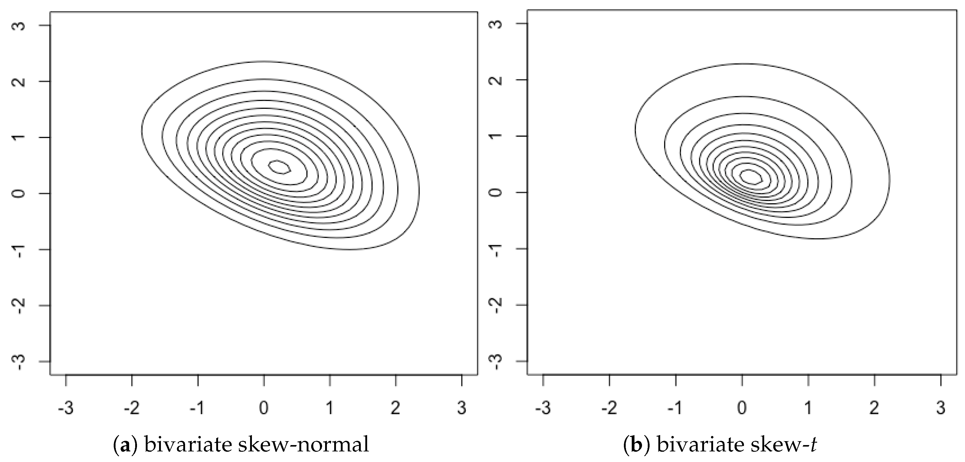
where $Q_x={(\mathbf{x}-\mathit{\mu })}^T{\mathsf{\Sigma }}^{-1}(\mathbf{x}-\mathit{\mu })$, $t_d(\mathbf{x};\nu )$ is the density of a d-dimensional t variate with $\nu$ degrees of freedom, and $T_1(x;\nu +d)$ is the skewing function and denotes the cdf of the scalar t-distribution with $\nu +d$ degrees of freedom. Figure 2 shows contour plots of the bivariate skew-t density along with the bivariate skew-normal.

The multivariate skew-t distribution is not closed under conditioning, which is important for methods that require the study of the conditional distribution of a skew-t. Also, although the skew-t distribution has the ability to model distributional tails that are heavier than the normal, it cannot represent lighter tails. A family of multivariate extended skew-t (EST) distributions which offers a solution for these issues has been introduced by Arellano-Valle and Genton [38]. Finally, we stress that the multivariate skew-t does not suffer from the above-mentioned Fisher information singularity.

4. (Multiple) Scale and Location-Scale Mixtures of Multinormal Distributions

In this section we describe four types of location–scale mixtures of multinormal distributions: the scale mixtures (Section 4.1), the location–scale mixtures (Section 4.2), the multiple scale mixtures (Section 4.3), and the multiple location–scale mixtures (Section 4.4). An alternative name from the literature for scale and location–scale mixtures is variance and mean-variance mixtures. For the sake of presentation, we only describe inferential issues related to the latter two families of distributions as they respectively encompass the former two.

4.1. Scale Mixtures of Multinormal Distributions

Scale mixtures of multinormal distributions are typically obtained via the stochastic representation

$$\mathbf{X}{=}_d\mathit{\mu }+\sqrt{W}\mathsf{\Lambda }\mathbf{Z},$$

(4)

where W is a non-negative scalar-valued random variable that is independent of $\mathbf{Z}$ and $\mathsf{\Lambda }{\mathsf{\Lambda }}^{\prime }=\mathsf{\Sigma }$, the scatter matrix. The scalar W is called weight variable and we denote its density by $f_W(·;\mathit{\theta })$ depending on some parameter $\mathit{\theta }\in {\mathbb{R}}^m$. In some sense, this weight variable plays the same role as $\mathcal{R}$ in the construction of elliptically symmetric distributions. The resulting density of the scale mixtures of multinormal distributions then is

$$\mathbf{x}\mapsto {\int }_0^{\infty }{\varphi }_d(\mathbf{x};\mathit{\mu },\mathsf{\Sigma }/w)f_W(w;\mathit{\theta })dw,$$

(5)

where we denote by ${\varphi }_d(\mathbf{x};\mathit{\mu },\mathsf{\Sigma })$ the density of the d-variate normal distribution with mean $\mathit{\mu }\in {\mathbb{R}}^d$ and positive-definite scatter matrix $\mathsf{\Sigma }\in {\mathbb{R}}^{d\times d}$.

Various choices of W have been explored in the literature, with special focus on Gamma distributions with density $x\mapsto \frac{{\gamma }^{\alpha }}{\mathsf{\Gamma }\left(\alpha \right)}{x}^{\alpha -1}exp(-\gamma x),x>0$, where $\alpha ,\gamma >0$ are respectively a shape and scale parameter. The multivariate t-distribution is for instance defined as Gaussian scale mixture based on a Gamma weight variable with parameters $\alpha =\gamma =\nu /2$. Gaussian mixtures of the form (5) still belong to the family of elliptically symmetric distributions, and suffer from the limitations mentioned in Section 2.2.

4.2. Location-Scale Mixtures of Multinormal Distributions

The limitations of elliptical symmetry can be overcome by considering location–scale mixtures instead of only scale mixtures. Replacing the fixed vector $\mathit{\mu }$ in (4) with a stochastic quantity $\mathbf{m}\left(W\right)$ where $\mathbf{m}:{\mathbb{R}}^{+}\to {\mathbb{R}}^d$ is a measurable function, we get the stochastic representation

$$\mathbf{X}{=}_d\mathbf{m}\left(W\right)+\sqrt{W}\mathsf{\Lambda }\mathbf{Z}.$$

A common specification for $\mathbf{m}\left(W\right)$ is $\mathit{\mu }+W\mathit{\xi }$ where $\mathit{\xi }\in {\mathbb{R}}^d$. Location-scale mixtures of multinormal distributions have the density

$$\mathbf{x}\mapsto {\int }_0^{\infty }{\varphi }_d(\mathbf{x};\mathbf{m}\left(w\right),\mathsf{\Sigma }/w)f_W(w;\mathit{\theta })dw.$$

The presence of w in the location parameter $\mathbf{m}\left(w\right)$ implies that location–scale mixtures of multinormal distributions are not elliptically symmetric. We refer the interested reader to Section 6.2 of McNeil et al. [39] for more details and references about scale and location–scale mixtures of multinormal distributions.

4.3. Multiple Scale Mixtures of Multinormal Distributions

A new family of scale mixtures of multinormal distributions has been proposed by Forbes and Wraith [40] and termed multiple scaled distributions. They replace the scalar weight variable W in (4) with a d-dimensional weight vector $\mathbf{W}={(w_1,\dots ,w_d)}^{\prime }$. To simplify their construction, Forbes and Wraith [40] decompose the matrix $\mathsf{\Sigma }$ into $\mathbf{D}\mathbf{A}{\mathbf{D}}^T$, where $\mathbf{D}$ is the matrix of eigenvectors of $\mathsf{\Sigma }$ and $\mathbf{A}$ is a diagonal matrix with the corresponding eigenvalues of $\mathsf{\Sigma }$. This leads to the stochastic representation

$$\begin{array}{c}\hfill \mathbf{X}{=}_d\mathit{\mu }+\mathbf{D}{\mathbf{A}}^{1/2}{\left[Z_1/\sqrt{W_1},\cdots ,Z_d/\sqrt{W_d}\right]}^T,\end{array}$$

(6)

where $Z_i,i=1,\dots ,d,$ are standardized Gaussian random variables and $W_1,\cdots ,W_d$ are d independent positive variables with respective densities $f_{W_i},i=1,\dots ,d.$ This extension brings more flexibility and, in particular, allows different tail weights in every direction. The decomposition of $\mathsf{\Sigma }$ into $\mathbf{D}\mathbf{A}{\mathbf{D}}^T$ allows an intuitive incorporation of the multiple weight parameters in the Gaussian density inside (5): ${\varphi }_d(\mathbf{x};\mathit{\mu },\mathbf{D}{\mathsf{\Delta }}_w\mathbf{A}{\mathbf{D}}^T)$, where ${\mathsf{\Delta }}_w=\mathrm{diag}(w_1^{-1},\cdots ,w_d^{-1})$. The generalization of the density of the scale mixture into the density of the multiple scale mixture is therefore defined as

$$\begin{array}{c}\hfill \mathbf{x}\mapsto {\int }_0^{\infty }\cdots {\int }_0^{\infty }{\varphi }_d(\mathbf{x};\mathit{\mu },\mathbf{D}{\mathsf{\Delta }}_w\mathbf{A}{\mathbf{D}}^T)f_{\mathbf{W}}(w_1,\cdots ,w_d;\mathit{\theta })d{w}_1\cdots d{w}_d,\end{array}$$

(7)

where $f_{\mathbf{W}}(w_1,\cdots ,w_d;\mathit{\theta })$ is now a d-variate density to be further specified, depending on a vector of parameters $\mathit{\theta }$. By considering independent weights, (7) can be written as

$$\begin{array}{c}\hfill \prod _{j=1}^d{\int }_0^{\infty }{\varphi }_1\left({\left[{\mathbf{D}}^T(\mathbf{x}-\mathit{\mu })\right]}_j;0,A_{jj}{w}_j^{-1}\right)f_{W_j}(w_j;{\mathit{\theta }}_j)d{w}_j,\end{array}$$

where ${\left[{\mathbf{D}}^T(\mathbf{x}-\mathit{\mu })\right]}_j$ denotes the j-th component of the vector ${\mathbf{D}}^T(\mathbf{x}-\mathit{\mu }),$${\mathit{\theta }}_j$ the vector of parameters relevant for $W_j$ and $A_{jj}$ the j-th diagonal element of the diagonal matrix $\mathbf{A}$.

The stochastic representation (6) is very useful for simulations as well as for the derivation of properties of multiple scaled distributions. For instance, moments can readily be derived from (6) and marginal distributions are easy to sample from. Note however that, in general, numerical integration is required to compute their pdfs.

Setting $f_{W_j}(w_j;{\mathit{\theta }}_j)$ to $\mathrm{Gamma}(w_j;{\nu }_j/2,{\nu }_j/2)$ leads to a generalization of the multivariate t-distribution with density

$$\mathbf{x}\mapsto \prod _{j=1}^d\frac{\mathsf{\Gamma }(({\nu }_j+1)/2)}{\mathsf{\Gamma }({\nu }_j/2){\left(A_j{\nu }_j\pi \right)}^{1/2}}{\left(1+\frac{{\left[{\mathbf{D}}^T(\mathbf{x}-\mathit{\mu })\right]}_j^2}{A_j{\nu }_j}\right)}^{-({\nu }_j+1)/2}.$$

This multiple scaled t-distribution allows for a number of different shapes which are not elliptically symmetric, though well centrally symmetric, as can be appreciated from Figure 3.

Parameter estimation by means of maximum likelihood can be performed via the EM algorithm, see Section 4 of Forbes and Wraith [40] for details. This estimation approach, however, happens to be very slow in high dimensions. The estimation of $\mathbf{D}$ is also problematic, as it is only identifiable up to a rotation. This implies that one has to make sure that, for instance, the eigenvalues are always ordered, as otherwise problems in the estimation of the degrees of freedom may appear.

4.4. Multiple Location-Scale Mixtures of Multinormal Distributions

In order to provide a wider variety of distributional forms, Wraith and Forbes [41] proposed an extension of their multiple scale mixtures to multiple location–scale mixtures of multinormal distributions. This extension allows different tail and skewness behavior in each dimension of the variable space with arbitrary correlation between dimensions. They replace $\mathit{\mu }$ in (6) with $\mathit{\mu }+\mathbf{D}{\mathsf{\Delta }}_{\mathbf{W}}\mathbf{A}{\mathbf{D}}^T\mathit{\beta }$ where $\mathit{\beta }\in {\mathbb{R}}^d$ is a skewness parameter. This yields densities of the form

$$\mathbf{x}\mapsto {\int }_0^{\infty }\cdots {\int }_0^{\infty }{\varphi }_d(\mathbf{x};\mathit{\mu }+\mathbf{D}{\mathsf{\Delta }}_{\mathbf{W}}\mathbf{A}{\mathbf{D}}^T\mathit{\beta },\mathbf{D}{\mathsf{\Delta }}_{\mathbf{W}}\mathbf{A}{\mathbf{D}}^T)\times f_{\mathbf{W}}(w_1,\cdots w_d;\mathit{\theta })d{w}_1\cdots d{w}_d,$$

where the weights are assumed to be independent: $f_{\mathbf{W}}(w_1,\cdots ,w_d;\mathit{\theta })=f_{W_1}(w_1;{\mathit{\theta }}_1)\cdots f_{W_d}(w_d;{\mathit{\theta }}_d).$ If $f_{W_m}(w_m;{\mathit{\theta }}_m)$ is the Generalised Inverse Gaussian (GIG) density, then $\mathbf{X}$ follows a generalization of the multivariate Generalised Hyperbolic distribution, the so-called multiple scaled generalised hyperbolic distribution (MSGH).

The multiple location–scale mixtures of multinormal distributions provide very flexible distributional forms. The parameter $\mathit{\beta }$ measures asymmetry and its sign determines the type of skewness. Each dimension can be governed by a different tail behavior. The marginals are easy to sample from, but computing their densities involves, in general, numerical integration. Estimation of the parameters can be done using the EM algorithm, bearing in mind however the identifiability issues and computational difficulties in high dimensions.

5. Multivariate Distributions Obtained via the Transformation Approach

The idea underpinning the transformation approach is quite simple: start from a “basic” random vector $\mathbf{Y}$, typically multivariate normal, and turn it into $\mathbf{X}{=}_d{\mathbf{H}}^{-1}\left(\mathbf{Y}\right)$ via some diffeomorphism $\mathbf{H}:{\mathbb{R}}^d\to {\mathbb{R}}^d$ (The reason for writing $\mathbf{X}{=}_d{\mathbf{H}}^{-1}\left(\mathbf{Y}\right)$ instead of the apparently more natural $\mathbf{X}{=}_d\mathbf{H}\left(\mathbf{Y}\right)$ can be traced back to the origins of this approach in Edgeworth (1898) who spoke of “Method of Translation” instead of transformation. The pre-dominance of the (scalar) normal distribution at that time implied that researchers were searching for a transformation to make their transformed data have a normal behaviour, hence $\mathbf{H}\left(\mathbf{X}\right)$ which follows the law of $\mathbf{Y}$). Writing f the density of $\mathbf{Y}$, the new random vector $\mathbf{X}$ has density $\mathbf{x}\mapsto f\left(\mathbf{H}\left(\mathbf{x}\right)\right)\left|D\mathbf{H}\left(\mathbf{x}\right)\right|,\mathbf{x}\in {\mathbb{R}}^d,$ where $D\mathbf{H}\left(\mathbf{x}\right)$ stands for the determinant of the Hessian matrix associated with the transformation $\mathbf{H}$. For instance, if $\mathbf{Y}$ follows a ${\mathbb{N}}_d(\mathit{\mu },\mathsf{\Sigma })$, then a transformation ${\mathbf{H}}_{\mathbf{a},\mathbf{b}}$ with $\mathbf{a}\in {\mathbb{R}}^d$ a skewness parameter and $\mathbf{b}\in {\mathbb{R}}^d$ a tail weight parameter leads to a multivariate distribution with well-identified location, scatter, skewness and tail weight parameters, where moreover the tail weight parameter is d-dimensional.

Ley and Paindaveine [36] study the transformation from a general viewpoint. Their focus lies on producing pure skewing mechanisms, hence their transformations only contain a skewness parameter. Theorem 3.2 of Ley and Paindaveine [36] details the impact on the tail behaviour of each skewing transformation.

5.1. Tukey’s Transformation

A well-known one-dimensional example of a transformation distribution is Tukey’s g-and-h distribution (Tukey [42], see also Hoaglin [43]). A standard normal random variable Z is transformed to $X{=}_d{\tau }_{g,h}\left(Z\right),$ where

$$\begin{array}{c}\hfill {\tau }_{g,h}\left(Z\right)=\left(\frac{exp\left(gZ\right)-1}{g}\right)exp\left(\frac{h}{2}{Z}^2\right),\end{array}$$

(8)

with $g\in \mathbb{R}$ and $h\ge 0.$ The resulting random variable X is said to have a g-and-h distribution, where g is a real constant controlling the skewness and h is a nonnegative real constant controlling the tail weight. Note that ${\tau }_{0,0}\left(Z\right)=Z$. The g-and-h distribution does not allow a closed-form density since ${\tau }_{g,h}$ does not possess a closed-form inverse, but the quantiles are explicitly available in terms of the quantiles of Z.

Field and Genton [2] extended the g-and-h distribution to the multivariate setting. A random vector $\mathbf{X}\in {\mathbb{R}}^d$ is said to have a standard multivariate g-and-h distribution, where $\mathbf{g}={(g_1,\cdots ,g_d)}^{\prime }\in {\mathbb{R}}^d$ controls the skewness and $\mathbf{h}={(h_1,\cdots ,h_d)}^{\prime }\in {\mathbb{R}}_{+}^d$ controls the tail weight, if it can be represented as

$$\mathbf{X}{=}_d{({\tau }_{g_1,h_1}\left(Z_1\right),\cdots ,{\tau }_{g_d,h_d}\left(Z_d\right))}^{\prime }={\mathit{\tau }}_{g,h}\left(\mathbf{Z}\right),$$

where $\mathbf{Z}={(Z_1,\cdots ,Z_d)}^{\prime }$ has a standard multivariate normal distribution and the univariate functions ${\tau }_{g_i,h_i},i=1,\dots ,d,$ are defined by (8). Location and scatter parameters can be introduced as usual, leading to the following stochastic representation:

$$\mathbf{X}{=}_d\mathit{\mu }+{\mathsf{\Sigma }}^{1/2}{\tau }_{\mathbf{g},\mathbf{h}}\left(\mathbf{Z}\right).$$

By construction, the marginals of ${\mathsf{\Sigma }}^{-1/2}(\mathbf{X}-\mathit{\mu })$ follow scalar g-and-h distributions. Just as its one-dimensional antecedent, the multivariate $\mathbf{g}$-and-$\mathbf{h}$ distribution does not have a closed-form density unless $\mathbf{g}=\mathbf{0}$, and one has to resort to some definition of quantiles to estimate its parameters. One issue of the multivariate $\mathbf{g}$-and-$\mathbf{h}$ distribution in higher dimensions is that the number of directions in which to compute the quantiles grows exponentially.

5.2. SAS Transformation

Another popular univariate transformation leads to the Sinh-Arcsinh (SAS) distribution of Jones and Pewsey [44], obtained by transforming a standard normal random variable by the inverse of the sinh-arcsinh function $z\mapsto S_{g,h}\left(z\right):=sinh(h{sinh}^{-1}\left(z\right)-g),z\in \mathbb{R},$ where $g\in \mathbb{R}$ is a skewness parameter and $h>0$ a tail weight parameter. After adding a location parameter $\mu \in \mathbb{R}$ and a scale parameter $\sigma >0$, the resulting SAS-normal or SAS density is of the form

$$x\mapsto \frac{h/\sigma }{\sqrt{2\pi (1+{(x-\mu )}^2/{\sigma }^2)}}{\left(1+S_{g,h}^2\left(\frac{x-\mu }{\sigma }\right)\right)}^{1/2}exp\left(-\frac{S_{g,h}^2\left(\frac{x-\mu }{\sigma }\right)}{2}\right).$$

Heavy-tailed distributions correspond to $h<1$ and light-tailed distributions to $h>1$, $h=1$ yielding normal-like tails. All non-zero values of g lead to skewed distributions. The SAS distribution enjoys numerous appealing properties such as parameter interpretability and straightforward parameter estimation, see Jones and Pewsey [44].

Jones and Pewsey [44] briefly described a multivariate extension of the SAS distribution (though they did not discuss inference). It is based on transforming the univariate marginals of a standardized, but correlated, multivariate normal distribution. Skewness and/or tail weight are modelled on the original scales of the variables. In d dimensions, let $\mathbf{R}$ be a correlation matrix and define the vector $\mathbf{X}$ by $Y_i{=}_d{S}_{g_i,h_i}\left(X_i\right),i=1,\cdots ,d,$ where $\mathbf{Y}\sim {\mathbb{N}}_d(\mathbf{0},\mathbf{R}).$ The density of $\mathbf{X}$ then is

$${\mathbf{x}\mapsto \{\left(2\pi \right)}^d{\left|\mathbf{R}\right|\}}^{-1/2}exp\{-S_{\mathbf{g},\mathbf{h}}{\left(\mathbf{x}\right)}^{\prime }{\mathbf{R}}^{-1}{S}_{\mathbf{g},\mathbf{h}}\left(\mathbf{x}\right)/2\}\prod _{i=1}^d\left\{{(1+x_i^2)}^{-1/2}{h}_i{\left(1+S_{g_i,h_i}^2\left(x_i\right)\right)}^{1/2}\right\}.$$

The univariate marginals are sinh-arcsinh distributions by construction, while conditional distributions are not very tractable. Figure 4 shows the contour plots of densities of bivariate SAS distributions.

6. Copula-Based Multivariate Distributions

Copulas are a very popular tool to build multivariate distributions as they allow modelling separately the marginal distributions and the dependence structure. According to Sklar’s Theorem [45], any multivariate cdf F with marginal distribution functions $F_1,\dots ,F_d$ can be expressed under the form

$$F(x_1,\dots ,x_d)=C(F_1\left(x_1\right),\dots ,F_d\left(x_d\right)),$$

(9)

where C is a copula, which means a cdf of a d-variate random vector uniformly distributed on the unit d-cube. Vice-versa, any combination of such a copula C and marginal distributions leads to a multivariate random vector with cdf $C(F_1\left(x_1\right),\dots ,F_d\left(x_d\right))$.

The idea underpinning the copula construction is that the random vector $\mathbf{U}{=}_d{(F_1\left(X_1\right),\dots ,F_d\left(X_d\right))}^{\prime }$, with $\mathbf{X}={(X_1,\dots ,X_d)}^{\prime }\sim F$, has uniform marginals and takes its values on the unit d-cube. The dependence structure of $\mathbf{X}$ thus is inherited from the dependence structure on the unit d-cube. This freedom of choice in combining the copula C with the marginal cdfs $F_1,\dots ,F_d$ is the main reason for the popularity of copulas. Their first appearance in the statistical literature is often traced back to Fréchet [46], and the cornerstone references about copulas are the monographs Joe [47] and Nelsen [6].

Simulation methods for copula-based multivariate distributions depend on the specific type of copula. The general approach for generating data from these types of distributions is to first sample from a specific copula C, that is ${(U_1,\cdots ,U_d)}^{\prime }\sim C$, and second obtain $\mathbf{X}$ using inverse marginal distributions, that is $X_i{=}_d{F}_i^{-1}\left(U_i\right)$.

Two famous families of copulas are Archimedean and elliptical copulas:

-

A d-variate Archimedean copula is the function

$$C(u_1,u_2,\cdots ,u_d)={\varphi }^{-1}(\varphi \left(u_1\right)+\cdots +\varphi \left(u_d\right)),{(u_1,\dots ,u_d)}^{\prime }\in {[0,1]}^d,$$

where $\varphi :[0,1]\to [0,\infty ]$ is continuous, decreasing, convex and such that $\varphi \left(1\right)=0.$ Such a function $\varphi$ is called a generator. An important source of generators for Archimedean d-copulas consists of the inverses of the Laplace transforms of cdfs. Examples of Archimedean copulas are the Gumbel, Clayton and Frank copula. We refer the interested reader to the above mentioned references for more details.

-

As the terminology suggests, elliptical copulas are the copulas of elliptically symmetric distributions. From (9) one readily sees that an elliptical copula is expressed as $F(F_g^{-1}\left(x_1\right),\dots ,F_g^{-1}\left(x_d\right))$ where F is the elliptical cdf and $F_g$ is the same symmetric marginal cdf for every component (see Section 2.1). They naturally inherit good properties as well as drawbacks from elliptical distributions. More detailed information about elliptical copulas is provided in the next section on Meta-Elliptical distributions as these are, de facto, nothing else but multivariate distributions obtained via elliptical copulas.

In high dimensions, the classical copula construction faces modelling limitations. The statistical community working on copulas has reacted to this bottleneck by devising vine copulas based on the pair-copula construction of Joe [48] and Aas et al. [49], and graph theory [50,51]. We do not enter into details here but refer the reader to Aas et al. [49] and the monograph Kurowicka and Joe [52]. An alternative approach to deal with high-dimensional data via copulas are the factor copulas described by Oh and Patton [53].

Parameter estimation in copulas can become challenging and various approaches have been proposed. The natural approach is maximum likelihood estimation for all parameters and the entire distribution, but it is often computationally unaffordable. Alternatively, a two-step procedure ought to be considered, where first the margins are estimated followed by the copula parameters. In both steps, maximum likelihood is used. A third approach is pseudo–maximum likelihood, which is also a two-step procedure where the marginals are estimated non-parametrically. We refer the reader to Embrechts and Hofert [54], who in particular discuss estimation in high dimensions, and Joe [47] for the asymptotics of the two-step approach.

6.1. Meta-Elliptical Distributions

As already mentioned, meta-elliptical distributions are in fact nothing else but distributions based on elliptical copulas. Fang et al. [55] coined the term as reference to the meta-Gaussian distribution of Krzysztofowicz and Kelly [56].

Let $\mathbf{Y}={(Y_1,\dots ,Y_d)}^{\prime }$ be an elliptically symmetric random vector with density (2) where $\mathit{\mu }=\mathbf{0}$ and $\mathsf{\Sigma }=\mathbf{R}$, the correlation matrix. In accordance with Fang et al. [55], we denote the identical marginal density and cdf respectively as $f_g(·)$ and $F_g(·)$. A random vector $\mathbf{X}={(X_1,\cdots ,X_d)}^{\prime }$ is then said to be meta-elliptical with the copula inherited from $\mathbf{Y}$ and marginal distributions $F_1,\dots ,F_d$ with densities $f_1,\dots ,f_d$ if we have the stochastic representation $X_i{=}_d{F}_i^{-1}\left(F_g\left(Y_i\right)\right)$ for all $i=1,\dots ,d$. This leads to the following density for $\mathbf{X}$:

$$\begin{array}{c}\hfill \mathbf{x}\mapsto \gamma (F_g^{-1}\left(F_1\left(x_1\right)\right),\cdots ,F_g^{-1}\left(F_d\left(x_d\right)\right);\mathbf{R})\prod _{i=1}^d{f}_i\left(x_i\right),\end{array}$$

where $\mathbf{x}={(x_1,\dots ,x_d)}^{\prime }$ and $\gamma$ is the d-variate density weighting function

$$\gamma (y_1,\cdots ,y_d;\mathbf{R})={\left|\mathbf{R}\right|}^{-1/2}{c}_{d,g}g\left({\mathbf{y}}^{\prime }{\mathbf{R}}^{-1}\mathbf{y}\right)/\prod _{i=1}^d{f}_g\left(y_i\right).$$

We borrow the name “density weighting function” from Fang et al. [55] and the reader should bear in mind that it refers to the density of the elliptical copula. Conditional distribution functions can easily be derived, as well as dependence properties like the Kendall’s correlation coefficient, see Fang et al. [55].

An interesting example of a meta-elliptical distribution is the multivariate asymmetric t-distribution proposed by Fang et al. [55]. Note that the terminology “asymmetric t-distribution”, taken from Fang et al. [55], is not conform with our definition of symmetry and asymmetry, since actually this distribution is centrally symmetric. Letting $t_m$ and $T_m$ respectively be the density and distribution functions of the scalar t-distribution with m degrees of freedom, its density reads

$$\mathbf{x}\mapsto \gamma (T_m^{-1}\left(T_{m_1}\left(x_1\right)\right),\cdots ,T_m^{-1}\left(T_{m_d}\left(x_d\right)\right);\mathbf{R})\prod _{i=1}^d{t}_{m_i}\left(x_i\right),$$

where

$$\begin{array}{cc}\hfill \gamma (y_1,\cdots ,y_d;\mathbf{R})=& \frac{\mathsf{\Gamma }((m+d)/2){\left(\mathsf{\Gamma }(m/2)\right)}^{d-1}}{{\left(\mathsf{\Gamma }((m+1)/2)\right)}^d}{\left|\mathbf{R}\right|}^{-1/2}{\left(1+\frac{{\mathbf{y}}^{\prime }{\mathbf{R}}^{-1}\mathbf{y}}{m}\right)}^{-\frac{m+d}{2}}\prod _{i=1}^d{\left(1+\frac{y_i^2}{m}\right)}^{\frac{m+1}{2}}.\hfill \end{array}$$

This distribution is said to have $(m;m_1,\cdots ,m_d)$ degrees of freedom and we use the notation $\mathbf{X}\sim AM{t}_d(m;m_1,\cdots ,m_d;\mathbf{R}).$ Of course, this asymmetric t-distribution and the classical t-distribution share the same copula, and the latter is retrieved for $m_1=m_2=\cdots =m_d=m$.

The $AM{t}_d$ distribution overcomes certain modelling limitations of the elliptically symmetric distributions since it is able to incorporate different tail weights in each direction. Figure 5 shows the densities of asymmetric t-distributions with different marginal degrees of freedom and correlation coefficients.

6.2. Our Proposal: t-Copula with SAS Marginals

To fully exploit the power of copulas, it is essential to combine a sound copula dependence structure, such as elliptical or Archimedean copulas, with versatile marginal distributions. Given the appealing properties of the univariate SAS distribution, we suggest to use them as marginal distributions in combination with the t-copula described in the previous section. We call the new distribution the t-SAS distribution.

Letting $f_{g_i,h_i}$ and $F_{g_i,h_i}$ respectively be the density and distribution functions of the scalar SAS distribution with parameters $g_i$ and $h_i$, $i=1,\dots ,d$, and using the notations from the previous section, the density of the t-SAS distribution reads

$$\mathbf{x}\mapsto \gamma (T_m^{-1}\left(F_{g_1,h_1}\left(x_1\right)\right),\cdots ,T_m^{-1}\left(F_{g_d,h_d}\left(x_d\right)\right);\mathbf{R})\prod _{i=1}^d{f}_{g_i,h_i}\left(x_i\right).$$

The only difference with respect to the asymmetric t-distribution thus are the marginals. This new distribution enjoys all desirable properties: it has a simple data generation mechanism, it can be symmetric or asymmetric (thanks to the SAS marginals instead of t marginals), where the degree of skewness can vary in every direction, the dependence structure is governed by the popular t-copula while the marginals can be light- or heavy-tailed, and it is multi-tailed. We illustrate the various shapes of the t-copula with SAS marginals in Figure 6.

The t-SAS and the multiple location–scale mixtures of multinormal distributions share the asymmetric and multi-tailed characteristics, which are key for this article, but a closer look reveals that these distributions deal with these characteristics differently. The main difference is that the t-SAS distinguishes between joint tail dependence (through the copula) and marginal tail thickness (through the marginal distributions). Put it differently, the copula allows to disentangle the tail thickness that is common to all the elements of the random vector and the tail thickness that is idiosyncratic to each element of the random vector. By contrast, the multiple location–scale mixtures of multinormal distributions estimate as many tail parameters as dimensions of the random vector, but do not explain the commonness in the tails.

7. Classification and Comparison of the Families

Our goal in this section is to compare in a systematic way and classify the distinct families presented in previous sections in terms of their degrees of flexibility. The comparison is based on relevant properties that a flexible multivariate distribution ought to possess. Clearly, these properties may appear subjective, and the reader may favour other properties. The history of flexible modelling itself tells us that the fathers of this field were not unanimous about what makes a flexible distribution “good”. We refer the reader to Section 2 of Ley [57] for an overview of the stormy beginnings of this research domain, especially the competition between Edgeworth and Pearson.

We now explain the motivations behind each chosen criterion, and in how far every distribution satisfies each criterion. Some criteria may not be fulfilled by all special cases of a family of distributions, so our comparison is to be understood as the potential that every family possesses. Two further remarks should be made: (1) we focus on the multivariate SAS distributions within the family of multivariate distributions obtained via the transformation approach, and (2) we omit copulas in general and rather focus on meta-elliptical distributions.

Table 1. Summary of our property-based comparison.

Family of Distributions	Simulation	Asymmetry	Tail	TD	TMD	PE
Spherical	✓	SS	ST	✓	✓	✓
Elliptical	✓	ES	ST	✓	✓	✓
Skew-elliptical	✓	AS	ST	✓	✓	✓
Scale mixtures	✓	ES	ST	✗	✗	(✓)
Location-scale mixtures	✓	AS	ST	✗	✗	(✓)
Multiple scale mixtures	✓	CS	MT	✗	✗	(✓)
Multiple location–scale mixtures	✓	AS	MT	✗	✗	(✓)
SAS transformation of multinormal	✓	AS	MT	✓	✓	✓
Meta-elliptical distributions	✓	CS	MT	✗	✓	(✓)

SS, ES, CS, AS denote spherical symmetry, elliptical symmetry, central symmetry and asymmetry, while ST and MT respectively represent single tail parameter and multiple tail parameters. TD stands for tractable density, TMD for tractable marginal density and PE for parameter estimation.

summarizes our comparison, which is based on the following six criteria: whether simulation is feasible, the degree of asymmetry, the flexibility to capture the tail behaviour (which we denote by single tail or ST versus multi tail or MT), the tractability of the density, the tractability of marginal distributions, and the easiness of estimation of the parameters. The criterion on asymmetry deserves further explanations, since there are different types of (a)symmetry. The simplest form of symmetry is spherical. A random vector $\mathbf{X}$ is spherically symmetric (SS) if and only if $\mathbf{X}-\mathit{\mu }{=}_d\mathbf{O}(\mathbf{X}-\mathit{\mu })$ for every $d\times d$ rotation matrix $\mathbf{O}$, is elliptically symmetric (ES) if $\mathbf{X}{=}_d\mathbf{A}\mathbf{Y}+\mathit{\mu }$ where $\mathbf{Y}$ is spherically symmetric about the origin and $\mathbf{A}$ is an arbitrary $d\times d$ matrix, and is centrally symmetric (CS) if $\mathbf{X}-\mathit{\mu }{=}_d-(\mathbf{X}-\mathit{\mu })$. A random vector $\mathbf{X}$ that does not satisfy these definitions of symmetry is asymmetric (AS). In Table 1 a checkmark indicates that a given property is satisfied (a checkmark between parentheses expresses a partial satisfaction), while a cross means the opposite.

Now we are ready to delve into the comparison and criteria:

• Simulation: In order to be able to simulate data from every distribution, we need to have a stochastic representation that underpins a data generating mechanism. All families but copulas enjoy a stochastic representation, and all families can be simulated.
• Asymmetry: It is natural to require from a flexible distribution to be able to capture asymmetry, all the more as the symmetric situation is then contained as a special case. Spherically and elliptically symmetric distributions are, by nature, spherically and elliptically symmetric, respectively. Scale mixtures of multinormal distributions are also elliptically symmetric, while multiple scale mixtures of multinormal distributions and meta-elliptical distributions are centrally symmetric. All other families are able to model skew phenomena via some skewness parameter and hence fully satisfy this criterion.
• Tail: Like skewness, tail weight ought to be governed by at least a d-dimensional vector allowing for one parameter per dimension. This criterion is not satisfied by the spherically and elliptically symmetric distributions as they only contain a one-dimensional tail weight parameter, and consequently also not by the skew-elliptical distributions as they are directly derived from them. The same holds true for scale and location–scale mixtures of multinormal distributions. The remaining distributions can all be termed multi-tail.
• Tractable Density: It is desirable for a distribution to possess a tractable density, be it for the sake of understanding the roles of the parameters, the development of stochastic properties or for parameter estimation purposes. By tractable we mean a density that can be written out explicitly without involving complicated functions such as integrals, for example. The families of spherically and elliptically symmetric distributions can be considered as very tractable (although they do possess complicated special cases such as the scale mixtures of multinormal distributions and the elliptical $\alpha -$stable distributions). The same holds then true for the skew-elliptical distributions. The multivariate SAS distribution also possesses a tractable density. All other distributions do not have tractable densities.
• Tractable Marginal Distributions: Multivariate distributions should possess tractable marginal laws, as often one is interested not only in the combined behavior of various components, but also in their individual behavior. Similarly, tractable conditional distributions are an asset. However, we did not emphasize the latter as special requirement since a tractable density combined with tractable marginals inevitably leads to tractable conditional distributions, even if the latter are not necessarily of a well-known form. We have seen that spherically and elliptically symmetric distributions are closed under linear transformations, hence they do satisfy this requirement. The multivariate SAS distribution has SAS marginals and the meta-elliptical distributions, being based on copulas, allow by construction to have full control over the marginals. Skew-elliptical distributions also enjoy tractable marginals [30]. The only families of distributions not completely satisfying this criterion are the (multiple) scale and location–scale mixtures of multinormal distributions, where it is not difficult to sample from the marginals but computing their density involves numerical integration.
• Parameter Estimation: It is essential to correctly estimate the parameters of each distribution, in particular by means of maximum likelihood estimation (for the sake of brevity, we do not consider here other estimation methods such as moment-based or Bayesian methods). This ensures that the distributions can serve their purpose in other inferential endeavours such as hypothesis testing. All considered families satisfy this criterion, albeit some require more special care, such as for instance the multiple scale or multiple location–scale mixture of multinormal distributions where an EM algorithm is required, or the $\alpha -$stable distribution that requires the use of the fast Fourier transform. In case of meta-elliptical distributions, recently more efficient maximum likelihood estimation methods have been proposed [58] that decompose the estimation into marginal estimation and dependence structure estimation.

On basis of this discussion and Table 1, we propose the following classification of the flexible multivariate families of distributions in terms of their degrees of skewness and tail behavior:

• spherically symmetric distributions (ST, SS)
• elliptically symmetric distributions and scale mixtures of multinormals (both ST, ES)
• skew-elliptical distributions and location–scale mixtures of multinormals (both ST, AS)
• multiple scale mixtures of multinormals and meta-elliptical distributions (both MT, CS)
• multiple location–scale mixtures of multinormals and SAS transformation of multinormal (both MT, AS)

We believe that this classification further enhances the understanding of multivariate distributions and can also be a useful guide for both theoreticians and practitioners.

8. Finite Sample Performance Comparison

We assess the fitting abilities in finite samples of a selected group of distributions from the aforementioned families: multivariate t-distribution, skew-t distribution, multiple scaled t-distribution, meta-elliptical asymmetric t-distribution, and t-copula combined with SAS marginals. We opt for these distributions as they all relate to the multivariate t-distribution, and hence are comparable.

To get a fair picture, we generate data from every distribution and fit all other distributions. The metric comparison is the Bayesian Information Criterion (BIC). We generate data for dimensions 2 and 5 and for sample sizes $n=100,1000$ and 10,000. The number of replications is 100, though the word “replication” deserves some comments. In all replications, the location and scatter parameters are the same, but we have chosen distinct values of skewness and tail weight in order to consider distinct scenarios. Simulations were coded in R 3.4.2 [59], and the packages sn [60], copula [61], QRM [62] and fitdistrplus [63] were used. The computer used is a MacBook Pro (Retina, 15-inch, Mid 2015), Processor 2.2 GHz Intel Core i7, Memory 16 GB 1600 MHz DDR3. The code is available upon request.

The results of our simulation study are shown in

Table 2. BIC scores and computation times (in seconds, minutes or hours)—dimension 2.

Fitted Distribution	Data Generator
	t	Skew-t	Multiple Scaled-t	Meta Elliptical-t	t-SAS
n = 100
t		787.0882	1274.422	731.9593	918.0995
		(20.50 s)	( 59.89 s)	(10.49 s)	(35.65 s)
skew-t	623.4148		1080.851	668.383	736.6848
	(3.43 s)		(3.86 s)	(3.09 s)	(4.20 s)
multiple scaled-t	620.7204	698.6299		667.6790	746.9414
	(4.07 min)	(3.54 min)		(3.63 min)	(4.12 min)
meta elliptical-t	617.5156	692.7963	1112.939		776.8259
	(12.10 s)	(1.02 min)	(4.29 min)		(3.10 min)
t-SAS	634.0599	694.6652	1075.957	667.4588
	(1.31 min)	(2.03 min)	(9.73 min)	(2.72 min)
n = 1000
t		7346.343	11891.12	7849.712	9847.058
		(16.62 s)	(23.56 s)	(17.45 s)	(55.87 s)
skew-t	6066.006		10513.17	6620.216	7361.205
	(13.74 s)		(14.54 s)	(14.07 s)	(15.58 s)
multiple scaled-t	6091.425	6706.059		6585.36	7490.495
	(46.58 min)	(33.01 min)		(37.33 min)	(45.10 min)
meta elliptical-t	6054.726	6609.865	10,945.42		7855.342
	(7.31 min)	(1.44 min)	(1.34 min)		(10.26 min)
t-SAS	6095.659	6553.907	10,434.28	6539.835
	(19.46 min)	(11.83 min)	(32.67 min)	(11.94 min)
n = 10,000
t		72,318.55	118,699.1	77,715.79	96,475.54
		(1.38 min)	(38.73 s)	(1.49 min)	(1.59 min)
skew-t	59,862.13		104,062.7	65,793.52	72,670.13
	(2.48 min)		(2.56 min)	( 2.79 min)	(2.87 min)
multiple scaled-t	60,211.49	66,097.17		65,624.49	74,064.37
	(6.65 h)	(7.001 h)		(7.92 h)	(8.90 h)
meta elliptical-t	59,845.96	65,078.95	108,362.4		77,732.89
	(11.59 min)	(12.92 min)	(29.52 min)		(1.44 h)
t-SAS	60,115.14	64,506.98	103,324.6	64,959.53
	(2.12 h)	(1.96 h)	(10.17 h)	(1.81 h)

and

Table 3. BIC scores (in seconds, minutes or hours)—dimension 5.

Fitted Distribution	Data Generator
	t	Skew-t	Multiple Scaled-t	Meta Elliptical-t	t-SAS
n = 100
t		2139.904	2910.327	2431.283	2568.123
		(19.13 s)	(8.71 s)	(12.81 s)	(12.35 s)
skew-t	1541.473		3067.713	2367.529	2050.565
	( 10.19 s)		(10.67 s)	(11.59 s)	(13.90 s)
meta elliptical-t	1530.399	1591.337	2487.038		2275.882
	(4.05 min)	(3.49 min)	(3.97 min)		(4.09 min)
t-SAS	1581.714	1638.517	2509.191	2157.801
	(6.12 min)	(7.14 min)	(6.74 min)	(6.92 min)
n = 1000
t		20,440.26	28,311.18	23,663.64	24,483.51
		(16.54 s)	(14.02 s)	(20.48 s)	(13.20 s)
skew-t	14,053.25		27,661.15	40,215.95	19,902.44
	(39.59 s)		(41.76 s)	(48.51 s)	(47.05 s)
meta elliptical-t	14,026.45	15,169.81	23,467.53		22,220.04
	(23.87 min)	(23.95 min)	(26.24 min)		(35.05 min)
t-SAS	14,161.15	15,367.83	23,475.92	21,409.75
	(53.33 min)	(55.97 min)	(56.59 min)	(1.01 h)
n = 10,000
t		201,314.9	280,266.2	238,979.6	245,145.6
		(1.57 min)	(1.67 min)	(1.96 min)	(1.62 min)
skew-t	139,361.6		298,194.7	338,688.8	197,373.4
	(6.38 min)		(6.58 min)	(7.51 min)	(7.94 min)
meta elliptical-t	139,317.2	149,850.3	231,530.1		222,997.3
	(4.53 h)	(4.69 h)	(4.59 h)		(6.03 h)
t-SAS	140,195.5	152,159.8	231,812.7	212,482.6
	( 9.35 h)	(9.15 h)	(8.88 h)	(9.96 h)

, along with the computation times in parentheses. The EM algorithm for estimating the parameters of the multiple scaled t-distribution is very slow in dimension 5, which, in combination with the parameter identifiability issue mentioned in Section 4, leads us to leave this distribution out as competitor in the 5-dimensional setting, but we kept it as data generator.

On basis of the results in Table 2 and Table 3 (where the best-fitting distributions are indicated in boldface), we can draw the following conclusions:

• The distributions based on the multivariate t-copula yield in general the best fit.
• For the dimension $d=2$, the t-copula combined with SAS marginals outperforms its competitors, especially for large sample sizes, while for $d=5$ the meta-elliptical asymmetric t provides the best fit.
• For data generated under the $t-$ SAS distribution, the skew-t exhibits the best performance, which is in line with the fact that it can capture skewness as opposed to the meta-elliptical asymmetric t that is centrally symmetric. In dimension 2, the multiple scaled t-distribution even outperforms the meta-elliptical asymmetric t in this case.
• In most situations where the meta-elliptical asymmetric t is the best, the t-copula combined with SAS marginals has a nearly as good BIC value.
• In no setting does the multivariate t-distribution provide the best fit, nor does the multiple scaled t-distribution.
• The meta-elliptical asymmetric t and t-SAS are copula-based models and they are computationally demanding for large sample sizes and dimensions. Hence, they have large computational times. The same holds for the multiple scaled-t, as the parameters are estimated using the EM algorithm; it has the largest computational times in dimension 2, as mentioned earlier.

9. Conclusions

We have described popular families of flexible multivariate distributions, with a focus on skewness and tails. We have compared them in terms of their theoretical properties as well as fitting abilities. This comparison allows the reader to draw his/her own conclusions regarding which family to use in which situation. A further aid in this endeavour is our newly proposed classification.

Although flexibility is a desirable property of a distribution, it comes with the risk of overfitting. Indeed, the more parameters a distribution possesses, the more flexible it becomes, at the cost of parameter interpretability and accuracy of the estimators (as well as estimation complexity) for finite samples. While we do not thoroughly discuss estimation in this work, the distributions discussed here have parameters that are fairly interpretable. In general terms, the distributions possess a d-dimensional vector of location parameters, a $d(d+1)/2$-dimensional matrix of scatter parameters, a d-dimensional vector of skewness parameters and a d-dimensional vector of tail weight parameters. In the simplest distributions, some of these vectors and matrices are not present, while in others, additional parameters exist (like in the copulas with a tail parameter in the copula function).

Further interesting issues remain to be explored and discussed. For instance, inference in high-dimensional situations is currently a hot topic, and adapted parameter estimation methods need to be devised especially for those distributions where EM algorithms are being used. Another extension is broadening the universe of families. For example, Arellano-Valle et al. [64] proposed multiple scale-shape mixtures of multivariate skew-normal distributions. Another example is to investigate the (uni)modality of the distributions considered. Finally, flexible distributions for multivariate data that take values on non-linear manifolds such as spheres or Stiefel manifolds (see Chapter 2 of [65] for examples) are worth researching on.