Reusing Source Task Knowledge via Transfer Approximator in Reinforcement Transfer Learning

Abstract

Transfer Learning (TL) has received a great deal of attention because of its ability to speed up Reinforcement Learning (RL) by reusing learned knowledge from other tasks. This paper proposes a new transfer learning framework, referred to as Transfer Learning via Artificial Neural Network Approximator (TL-ANNA). It builds an Artificial Neural Network (ANN) transfer approximator to transfer the related knowledge from the source task into the target task and reuses the transferred knowledge with a Probabilistic Policy Reuse (PPR) scheme. Specifically, the transfer approximator maps the state of the target task symmetrically to states of the source task with a certain mapping rule, and activates the related knowledge (components of the action-value function) of the source task as the input of the ANNs; it then predicts the quality of the actions in the target task with the ANNs. The target learner uses the PPR scheme to bias the RL with the suggested action from the transfer approximator. In this way, the transfer approximator builds a symmetric knowledge path between the target task and the source task. In addition, two mapping rules for the transfer approximator are designed, namely, Full Mapping Rule and Group Mapping Rule. Experiments performed on the RoboCup soccer Keepaway task verified that the proposed transfer learning methods outperform two other transfer learning methods in both jumpstart and time to threshold metrics and are more robust to the quality of source knowledge. In addition, the TL-ANNA with the group mapping rule exhibits slightly worse performance than the one with the full mapping rule, but with less computation and space cost when appropriate grouping method is used.

1. Introduction

Reinforcement learning (RL) is a popular learning paradigm for solving sequential decision-making problems. However, it relies on extensive interactions with the environment to converge to an acceptable policy, which usually takes quite a long time. Therefore, techniques like transfer learning (TL) have been developed to facilitate the learning process and improve the performance in reinforcement learning. Based on the idea that the learned knowledge in a related source task may aid the learning process in the target task, transfer learning is gaining more and more attention, especially in some data mining domains like classification, regression and clustering. However, the work of the transfer learning under the reinforcement learning framework is relatively less. Therefore, this paper will focus on the transfer learning for reinforcement learning, not on the classification, regression and clustering problems.

In transfer learning, the target task is related to but different from the source task. Typically, the target task is more complex than the source task, and they are even characterized by different space/action spaces. Therefore, the source task knowledge can not be used directly in the target task. Typically, an inter-task mapping [1] is necessary; this consists of a state-mapping and an action-mapping, and it is able to map the source knowledge to the target task for initialization or other uses. Two issues stand out regarding the inter-task mapping. First, the inter-task mapping is typically designed by human experts, which can involve a lot of human resources. Second, methods to learn the inter-task mapping are almost all designed to learn just one-to-one mapping, which can not make full use of related features. To avoid the trouble of inter-task mapping, some TL methods just assume that the inter-task mapping is already given or that the source task and target task are from the same domain where no inter-task mapping is needed, but these assumptions may not hold in many cases.

Apart from the concerns on the inter-task mapping, there is another concern regarding the timing of transfer. Mostly, the transfer is done at the beginning of the reinforcement learning, which uses the source knowledge to initialize the target task. Works that done the transfer during the process of the reinforcement learning are very limited and may need extra parameter training at the same time.

The motivation of this paper is to reduce human involvements in the transfer learning, and to make a better use of the related features between the source task and the target task. This paper neither neglects the difference between the source task and the target task, nor assumes that the inter-task mapping is already given. Moreover, this paper also concerns the transfer learning happening during the reinforcement learning, but without extra parameter training during the reinforcement learning.

With these motivations, this paper makes a number of contributions by proposing a new transfer learning framework. This framework builds a transfer approximator to predict the quality of target task actions based on source task knowledge, and then biases the action selection of the target task learner with the Probabilistic Policy Reuse (PPR) scheme [2,3].

The main contributions of this work are as follows:

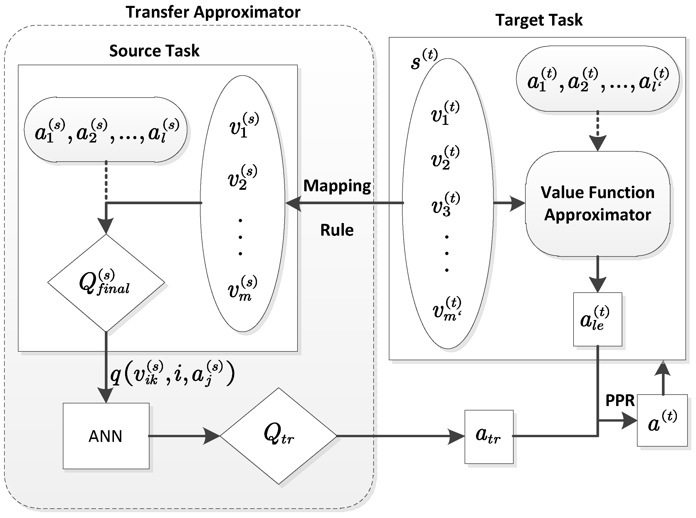
• The concept of the transfer approximator is proposed. By taking the state from the target task as the input and predicting the quality of actions in the target task, the transfer approximator does not need the action mappings across the two tasks. As for the state mapping in the inter-task mapping, it is replaced by the state feature mapping rules that are different from the state mapping of the inter-task mapping to some extent.
• Two mapping rules called full mapping and group mapping are designed. The mapping rule is used in the transfer approximator for mapping each state feature of the target task into a set of features in the source task. With such feature mapping rules, much more related feature information can be used. Differently from the state mapping of the inter-task mapping, the full mapping rule is totally task independent and human-free. However, it is hard for the group mapping rule to be task independent, but it can have relatively less human involvement depending on the grouping method used. For example, there will be nearly no human involvement if the grouping is done by certain machine learning methods.
• A new transfer learning framework, called Transfer Learning via Artificial Neural Network Approximator (TL-ANNA), is proposed. It builds an Artificial Neural Network (ANN) transfer approximator to transfer the related knowledge from the source task to the target task and reuses the transferred knowledge based on the PPR scheme. The ANNs are used to predict the quality of actions in the target task, which allows certain errors in collecting source knowledge and increases the robustness of transfer learning. The result from the transfer approximator is combined with the PPR scheme. Without extra parameter training during the RL of the target task, the PPR scheme provides easy integration between transferred knowledge and learned knowledge.

The rest of the paper is organized as follows. Related literature works are commented in Section 2. Section 3 outlines the concepts behind the reinforcement transfer learning. Section 4 details the proposed transfer learning framework. Experiments are presented in Section 5. Section 6 concludes the proposed methods.

2. Literature Review

Since the inter-task mapping is important in typical transfer leaning, some research focuses on the design of the inter-task mapping, such as [4]. However, human designed inter-task mapping involves too much human effort and can create inaccuracies due to the limitations of human knowledge, and many researchers have tried to autonomously learn inter-task mapping. The MASTER (Modeling Approximate State Transitions by Exploiting Regression) method proposed in [5] learns a one-to-one state mapping and action mapping by minimizing the MSE (Mean Square Error) between the mapped samples and the predicted samples in the target task. To remove the need of samples in the target task, Silva et al. [6] proposed the Zero-Shot Autonomous Mapping Learning to learn the state mapping between tasks described through Object-Oriented Markov Decision Process, where the action mapping is assumed to be given already. Instead of learning the inter-task mapping, some methods attempt to create other forms of inter-task mapping. A many-to-many inter-task mapping in the form of ANN was designed in our previous work [7].

The primary contrast between these previous methods and our work is that we are interested in relating more state features in the source task with that of the target task to make a better use of the related knowledge, and reducing the necessity of human involvements in the inter-task mapping, as well as trying to remove part of the inter-task mapping, such as the action mapping.

Some other research focuses on how to use the source knowledge but is based on some assumptions about the inter-task mapping. For instance, Wang and Taylor [8] used Gaussian Processes to summarize demonstrated policy (source knowledge) with the assumption that the inter-task mapping has been given. Brys et al. [9] encoded the transferred policy as a dynamic potential-based reward shaping function with the inter-task mapping assuming to exist already. The work [10] transferred the unchanged part between the source task and the target task, ignoring the need of the inter task mapping. The online transfer framework proposed in [11] uses advice as transferred knowledge, but the difference between tasks was not emphasized. The work [12] treated the source task and the target task as one single problem, so no consideration on the inter-task mapping was given. To avoid the need of inter-task mapping, Laflamm [13] chose the source task and the target task from the same domain with the same state and action space, and then compared three existing transfer learning methods on the Mario AI domain. The work in [14] transfers the shared transition sample $(s,a,r,s^{\prime })$ between tasks by modifying the immediate reward r with the estimated reward function, which is based on the assumption that the tasks only have different reward functions. The work in [15] proposed a new method called target transfer Q-Learning to transfer the Q-function when certain safe conditions are satisfied, where the two Markov Decision Processes (MDPs) have only different transition function, reward function and discount factor. The transfer learning method proposed in the work [16] uses the modified learning vector quantization (LVQ) to extract an abstract policy from the source task, where the state space and action space between tasks are the same.

Differently from above works, this work allows for the difference between the source task and the target task, and with no ignorance on the fact that the source knowledge can not be used directly in the target task. That is to say, the state space and the action space in the source task are both different from those in the target task. Furthermore, no inter-task mapping is assumed to be given to our transfer learning.

Apart from the inter-task mapping, some research tries to find other ways to relate the source task knowledge with the target task. The work in [17] uses the Transfer Component Analysis (TCA) to extract the features shared by visual observations in both simulations and real environments to do the transferring. By encoding the states as an image and the action space as a multi-channel image, the work in [18] introduced a novel state-action space representation that remains invariant to the number of agents in an environment for the policy transfer. The work [19] trained an invariant feature space to add additional terms to the reward function of the target agent. Successor features were used in the work [20] to parametrize the reward function with reward features, and the transfer was done by training the weights for these reward features. Shoeleh and Asadpour [21] added the learned skills to the target agent’s action repertoire by expanding the action-value function in the target task. The TL method proposed in [22] uses an inter-task mapping provided by the Unsupervised Manifold Alignment (UMA) technique to move back and forth between tasks to determine a policy adjustment term with the target apprentice learning, and then augments the transferred policy with the policy adjustment term for the transfer adaption. Kelly and Heywood [23] introduced a symbiotic framework that hierarchically constructs a policy tree to transfer tasks under genetic programming. Didi and Nitschke [24] used the neuro-evolution method to evolve policy from the source task to the target task. The ADAAPT (A Deep Architecture for Adaptive Policy Transfer) method proposed in [25] combines the weighted learned policies for knowledge transfer, and updates an attention work during the reinforcement learning to adjust the policy weights.

These methods either use specific representation in the task, or add some changes on the reward or action-value function, or learn some extra parameters in the target task along with the reinforcement learning. On the contrary, the proposed methods in this paper use a transfer approximator to find out the relationship between tasks before the transfer, and transfer knowledge during the reinforcement learning, without the need of specific representation in tasks or extra parameter learning during the transfer.

There is another big difference between the proposed methods and the reviewed works. Most previous transfer learning happens at the initialization period of the reinforcement learning. Some other works transfer during the reinforcement learning, but they either need extra parameter learning along with the transfer (e.g., [25]), or transfer with a budge or in certain circumstances [11]. On the contrary, the PPR scheme ([2,3]) is used in this paper to transfer knowledge, which adjusts the transferring by decaying probability during the reinforcement learning, and no extra parameter learning is needed during the transferring.

3. Reinforcement Transfer Learning

3.1. Reinforcement Learning

A Reinforcement Learning (RL) [26] problem is typically formalized as a Markov Decision Process (MDP) $[\mathcal{S},\mathcal{A},\mathcal{T},\mathcal{R}]$. The agent selects an action $a\in \mathcal{A}$ when it is in the environment’s state $s\in \mathcal{S}$. After taking the action a, it receives an immediate reward $r\in \mathcal{R}$, while the environment state transits into the next state $s^{\prime }\in \mathcal{S}$ with probability ${\mathcal{T}}_{s{s}^{\prime }}^a$. The agent’s goal is to maximize the total amount of reward it receives, which is often estimated by action-value function $Q^{\pi }(s,a)$, where $\pi :\mathcal{S}\to \mathcal{A}$ is the policy that the agent follows. The definition of the action-value function $Q^{\pi }(s,a)$ is as follows:

$$Q^{\pi }(s,a)=E_{\pi }\left\{\left.\sum _{k=0}^{\infty }{\gamma }^k{r}_{t+k+1}\right|s_t=s,a_t=a\right\},$$

(1)

where $0\le \gamma \le 1$ is the discount rate.

Solving a reinforcement learning task is to find the optimal policy ${\pi }^{*}$. By solving the Bellman optimality equation (Equation (2)), the optimal action-value function $Q^{*}$ can be obtained and therefore the optimal policy ${\pi }^{*}$ as well:

$$Q^{*}(s,a)=\sum _{s^{\prime }}{\mathcal{T}}_{s{s}^{\prime }}^a\left[r+\gamma \underset{a^{\prime }}{max}{Q}^{*}(s^{\prime },a^{\prime })\right].$$

(2)

However, in systems where the dynamics of the environment are unknown ($\mathcal{R}$ and/or $\mathcal{T}$) or where the state space ($\mathcal{S}$) and/or action space ($\mathcal{A}$) contain continuous variables, the Bellman optimality equation should be solved approximately. The temporal-difference (TD) learning methods with function approximation are popularly used in solving such RL problems. In this work, the proposed TL methods are based on the $Sarsa(\lambda )$ TD method with the CMAC (cerebellar model arithmetic computer, [27]) function approximator.

The CMAC is a linear tile-coding function approximator. It discretizes the continuous state space by laying infinite axis-parallel tilings over state variables and then generalizes them via multiple overlapping tilings with some offset. Each element of a tiling is called a tile, which is a binary feature. The value of a tile is 1 when being activated; otherwise, it is 0. The number of tilings and the tile width are hand-coded since they can influence the generalization. The CMAC maintains $Q(s,a)$ in the following form:

$$Q(s,a)={\overrightarrow{\theta }}^T{\overrightarrow{\varphi }}_a(s)=\sum _{i\in I({\overrightarrow{\varphi }}_a(s))}\theta (i),$$

(3)

where ${\overrightarrow{\varphi }}_a(s)$ is the vector of tile values for all the tiles that are laid for pair $(s,a)$, and $\overrightarrow{\theta }$ is the vector of tile weights for corresponding tiles. $I({\overrightarrow{\varphi }}_a(s))$ is the set of tiles that are activated by the pair $(s,a)$, whose tile values are 1.

For a state space with many state features, one-dimensional tilings are usually used, where each state feature can independently activate one tile in each tiling. Let ${\theta }_{ki}$ denote the weight for the tile activated in the ith tiling by the kth state feature and the action a, and let n denote the number of tilings. In this paper, the concept of the q-value function can be defined as $q(v_k,k,a)={\sum }_{i=1}^n{\theta }_{ki}$. Therefore, for a state with m state features, Equation (3) can be rewritten in the following form:

$$Q(s,a)=\sum _{k=1}^m\sum _{i=1}^n{\theta }_{ki}=\sum _{k=1}^{m}q(v_k,k,a),$$

(4)

where ${\theta }_{ki}$ is updated by the TD learner with samples from experience. Therefore, the q-value function $q(v_k,k,a)$ is what the kth state feature contributes to the action-value function Q.

The gradient-descent method is used to adjust the parameter $\theta$. The updating rule is as follows:

$${\overrightarrow{\theta }}_{t+1}={\overrightarrow{\theta }}_t+\alpha {\delta }_t{\overrightarrow{e}}_{(s_t,a_t)},$$

(5)

where $\overrightarrow{e}$ is eligibility trace [26], and ${\delta }_t$ is the usual TD error,

$${\delta }_t=r_{t+1}+\gamma Q_t(s_{t+1},a_{t+1})-Q_t(s_t,a_t).$$

(6)

3.2. Transfer Learning

In the target task without transfer learning, the RL learner initializes all the CMAC parameters ${\theta }^{(t)}$ with 0. Therefore, the target task learner can not distinguish the actions by the initial action-value function $Q_0^{(t)}$. As the RL learner interacts with the environment to collect samples, the distinctions between actions become clearer. Therefore, the learning process can be denoted as

$$\left(S^{(t)},s_0^{(t)},A^{(t)},T^{(t)},R^{(t)},Q_0^{(t)},{\pi }_0^{(t)}\right)\stackrel{D^{(t)}}{\Rightarrow }\left(Q_{final}^{(t)},{\pi }_{final}^{(t)}\right),$$

(7)

where $D^{(t)}$ is the knowledge received during the learning process. $Q_{final}^{(t)}\approx {(Q^{*})}^{(t)}$, which is learned approximately by adjusting parameters ${\theta }^{(t)}$ with $D^{(t)}$, and ${\pi }_{final}^{(t)}\approx {({\pi }^{*})}^{(t)}$.

In transfer learning, the source task has completed the RL process, as denoted in Equation (8). The idea of transfer learning is to reuse $D^{(s)}$, or $Q_{final}^{(s)}$, or ${\pi }_{final}^{(s)}$ to aid the learning process in the target task:

$$\left(S^{(s)},s_0^{(s)},A^{(s)},T^{(s)},R^{(s)},Q_0^{(s)},{\pi }_0^{(s)}\right)\stackrel{D^{(s)}}{\Rightarrow }\left(Q_{final}^{(s)},{\pi }_{final}^{(s)}\right).$$

(8)

There are many ways to realize transfer learning, and most of these methods need the inter-task mapping to map related knowledge from the source task into the target task. An inter-task mapping $\rho$ consists of a state mapping ${\chi }_X:s^{(t)}\leftarrow s^{(s)}$ and an action mapping ${\chi }_A:a^{(t)}\leftarrow a^{(s)}$. Typically, the inter-task mapping is either provided by human experts or learned via certain methods. Inter-task mapping provided by human experts involves too much human intervention and can bring in errors due to limitations of human knowledge. Methods to learn an inter-task mapping are usually complex and may cause much time and space consumption. Therefore, a TL method that can reduce and even eliminate the human involvement or remove some part of the inter-task mapping is very much worth studying. The concept of the transfer approximator is proposed in this paper to achieve these goals.

Typically, transfer learning methods with inter-task mapping $\rho$ use the mapped source knowledge to initialize the parameters in the target task to set a better start point for the RL learner in the target task. Supposing the knowledge transferred is an action-value function, this class of TL methods can be formalized as:

$$Q_0^{(t)}\left(s^{(t)},a^{(t)}\right)=Q_{final}^{(s)}\left({\chi }_X(s^{(t)}),{\chi }_A(a^{(t)})\right)=\rho \left(Q_{final}^{(s)}\right).$$

(9)

However, it is considered in this paper that the transferred knowledge not only can be used for initialization before the RL process but also can be helpful for biasing the learning during the RL process. Therefore, the PPR scheme is used in this paper to integrate transferred knowledge from the transfer approximator into the learned knowledge during the RL process, which can be formulated as:

$$Q^{(t)}\left(s^{(t)},a^{(t)}\right)\leftarrow g\left(f(Q_{final}^{(s)}),Q^{(t)}(s^{(t)},a^{(t)})\right),$$

(10)

where function f is realized by the transfer approximator in the proposed methods and function g is fulfilled by the PPR scheme. this class of methods aim at a fuller use of the transferred knowledge by using it not for initialization but for biasing during the learning process. The details of the proposed methods are presented in the following section.

4. Transfer Learning via ANN Approximator

In this paper, a novel transfer learning framework is proposed for reinforcement learning. This framework builds a component, namely transfer approximator, to leverage source knowledge and biases the action selection in the target task with PPR ( Probabilistic Policy Reuse) [2,3], as shown in Figure 1.

The main part of the proposed framework is a component which takes the state ($s^{(t)}$) of the target task as input and gives the target task a suggested action based on the predicted quality of target task actions. In this sense, this component is similar with the action-value function approximator of the RL in the target task, which also takes the state $s^{(t)}$ as the input and gives the agent an action $a_{le}^{(t)}$ based on the action-value $Q^{(t)}$. Therefore, the name Transfer Approximator is invented in this paper for this component. The predicted quality of target task actions from the transfer approximator are called the transferred action-value function $Q_{tr}\left(a^{(t)}\right)$, which is used to determine an action. This target task action determined by the transfer approximator is called the transferred action in this paper, denoted by $a_{tr}$. Since the transferred action $a_{tr}$ is already a target task action, it can be used in the target task directly, and no action mapping is needed even if the action set of the target task is different from that of the source task. Algorithm 1 demonstrates how an ANN transfer approximator works. In line 2 of Algorithm 1, a certain mapping rule is needed for the feature mapping. Compared with the state mapping in the inter-task mapping, the mapping rule used here has less and even no human involvements and can be more and even totally task independent. Line 4 is used for activating related source knowledge. Here, the q-value function from $Q_{final}^{(s)}$ is chosen as the related source knowledge. Each output node of the ANNs predicts a value of $Q_{tr}\left(a^{(t)}\right)$ corresponding to an action in the target task. The ANNs should be trained before transfer learning with a small set of samples from both the source task and target task.

Algorithm 1 The process in an ANN transfer approximator

Input:$s^{(t)}$ Output:$a_{tr}$  1: for each feature $v_k^{(t)}$ in $s^{(t)}$ do  2: Map $v_k^{(t)}$ into a set of features ($F_k^{(s)}$) in the source task  3: for each feature $v_{ik}^{(s)}\in F_k^{(s)}$ and each action $a_j^{(s)}\in {\mathcal{A}}^{(s)}$ do  4:  Activate related source knowledge (q-value function $q\left(v_{ik}^{(s)},i,a_j^{(s)}\right)$ from $Q_{final}^{(s)}$)  5: end for  6: end for  7: Use all the q-value functions obtained as the inputs of the ANNs  8: Predict the quality of the target task actions (denoted by $Q_{tr}$) with ANNs  9: $a_{tr}={arg\; max}_{a^{(t)}}{Q}_{tr}\left(a^{(t)}\right)$

Since there is a learned action $a_{le}^{(t)}$ determined from the value function approximator in the target task and a transferred action $a_{tr}$ determined from the transfer approximator, the PPR scheme can be used to determine the executing action $a^{(t)}$ for the RL learner in the target task.

As the transfer approximator in this work uses ANNs for prediction, this proposed algorithm is referred to as Transfer Learning via ANN Approximator (TL-ANNA). It has advantages over most of the TL algorithms mainly in terms of the following two aspects:

• With the use of the transfer approximator, TL-ANNA removes the need of the action mapping in the inter-task mapping. The state feature mapping rule in the transfer approximator can make a better use of the related knowledge in the source task than the typical one-to-one state mapping from a inter-task mapping does. Certain state feature mapping rules in the transfer approximator can even eliminate the human involvement.
• By combining the PPR scheme with the transfer approximator, TL-ANNA can integrate the source knowledge during the RL process, not just before the RL process.

Two state feature mapping rules for the transfer approximator, full mapping and group mapping, are designed in this paper. The structure of the ANNs varies due to the difference of the mapping rules. In the following subsections, we will introduce these two state feature mapping rules and the construction of the ANNs, as well as the biasing action selection scheme.

4.1. State Feature Mapping Rules

Denote the number of state features in the source task and the target task by m and $m^{\prime }$, respectively. The number of actions in the source task and the target task are denoted by l and $l^{\prime }$, respectively. Since the target task is usually more complex than the source task, it can be assumed that $m\le m^{\prime }$ and $l\le l^{\prime }$.

As described in Section 3, each state feature activates tiles independently when one-dimensional tile coding is used. For a tile coding that lays n tilings for a state, each state feature can activate one tile in each tiling independently and thus n tiles in total for the tile coding. Based on this independence, the concept of the state feature mapping rule is defined. Given a state $s^{(t)}=\left[v_1^{(t)},v_2^{(t)},\dots ,v_k^{(t)},\dots ,v_{m^{\prime }}^{(t)}\right]$ of the target task, the state feature mapping rule can map each feature $v_k^{(t)}$ to a set of state features in the source task and sets all the source task state features in the mapped set with the value of state feature $v_k^{(t)}$.

The two designed mapping rules are called Full Mapping and Group Mapping. Both mapping rules only map state features, while the typical inter-task mapping usually consists of state mapping and action mapping. The transfer approximator removes the necessity of an action mapping. Moreover, both state feature mapping rules are one-to-many mapping, while most of the state mappings in the inter-task mappings are just one-to-one mapping. Therefore, more related knowledge in the source task can be used in the transfer approximator. The full mapping rule is totally task independent, while the group mapping rule and the inter-task mapping are task related. In addition, the full mapping rule does not need human involvement, and the group mapping rule may also need no human involvement in certain circumstances, while many other inter-task mapping involves human effort. In the group mapping, the grouping not only can be done by human knowledge, but also can be done by some machine learning methods, such as clustering methods. However, the grouping methods are considered to be out of the scope of this paper and can be left for the future work.

4.1.1. Full Mapping

In this mapping rule, each state feature in $s^{(t)}$ is mapped into all the state features in the source task. That is to say, when mapping the kth feature of $s^{(t)}$, all the m state features in the source task are set with the value of $v_k^{(t)}$. Therefore, a target task state $s^{(t)}$ can be mapped into $m^{\prime }$ sets of features, and each mapped feature set consists of m source task features with all the same values of the corresponding target task feature. Given an action $a_j^{(s)}$ in the source task, each mapped source task feature $v_{ik}^{(s)}$ for the kth target state feature can activate n tiles in the tilings. Summing the weight of these n tiles, the corresponding q-value function $q\left(v_{ik}^{(s)},i,a_j^{(s)}\right)$ can be obtained. Therefore, a given target task state $s^{(t)}$ can activate $N_f$ sets of tiles and obtain $N_f$ pieces of q-value from the source task, where $N_f$ is given in Equation (11):

$$N_f=m^{\prime }\times m\times l.$$

(11)

4.1.2. Group Mapping

This mapping rule is based on the idea from our previous work [4]. Assume the state features from both the source task and the target task can be divided into K groups. Let $F_i^{(s)}$ and $F_i^{(t)}$ denote the ith group of features in the source and target task, respectively. The features in $F_i^{(t)}$ are all assumed to be related to all the features in $F_i^{(s)}$ but have no relationship (or little relationship) with features in other groups of the source task. Therefore, features from group $F_i^{(t)}$ simply need to be mapped into features in $F_i^{(s)}$. Supposing that $F_i^{(t)}$ has $m_i^{\prime }$ features and $F_i^{(s)}$ has $m_i$ features, a target task feature $v_k^{(t)}\in F_i^{(t)}$ can be mapped into $m_i$ source state features. Given an action $a_j^{(s)}$ in the source task, target task feature $v_k^{(t)}$ can activate $m_i$ sets of tiles. Therefore, a given target task state $s^{(t)}$ can activate $N_g$ sets of tiles and get $N_g$ pieces of q-value from the source task, where $N_g$ is given in Equation (12):

$$N_g=\sum _{i=1}^K(m_i^{\prime }\times m_i)\times l.$$

(12)

Note that, when $K=1$, the group mapping is equal to the full mapping. Full mapping does not require any grouping knowledge, which makes it totally task independent. However, full mapping requires much computation and space in complex tasks. Therefore, with additional knowledge (grouping knowledge), the full mapping can be changed into group mapping, which would reduce computation and space consumption. However, the grouping knowledge may come with the price of extra computing from methods like clustering, or extra human involvement in the grouping.

4.2. Construction of the ANNs

There are many kind of ANNs existing; however, the research on the ANNs is out of the scope of this paper. This paper adopts a simple structure of ANNs to demonstrate how the proposed transfer learning framework works, since the scale of training data is relatively small. However, in more complex problems with too many states and actions, more complex ANNs can be used and methods for accelerating ANNs [28,29] can be explored, which we will leave for future works. The BackPropagation (BP) ANNs with one hidden layer are chosen as the architecture of the ANNs in the transfer approximator. The ANNs take the source knowledge (q-value functions) obtained through the feature mapping rule as its inputs and predict the transferred action-value function $Q_{tr}$. The number of input nodes is $N_i$, which is given by Equation (13):

$$N_i=\sum _{i=1}^K(m_i^{\prime }\times m_i)\times l.$$

(13)

$K=1$ when full mapping is used. The number of input nodes is equal to the number of the q-value functions obtained from the source task. The number of output nodes is equal to the number of actions in the target task. Denote the number of output nodes by $N_o$; then,

$$N_o=l^{\prime }.$$

(14)

The predicted value from each output node indicates the quality of the corresponding action in the target task. In this way, it removes the necessity of the action mapping. The number of hidden nodes is denoted by $N_h$.

Suitable ANNs for the transfer approximator can be obtained through Algorithm 2, where T is a small number and $d_t^{(t)}$ is other related information in addition to the state $s_t^{(t)}$, the action $a_t^{(t)}$ and the reward $r_t^{(t)}$.

For each sample $(s_t^{(t)},a_t^{(t)},r_t^{(t)},d_t^{(t)})$ recorded from the target task, the $s_t$ is used to generate the input sample of the ANNs, while $(a_t^{(t)},r_t^{(t)},d_t^{(t)})$ are used to generate the corresponding output sample of the ANNs. The process of generating training samples will be detailed in the following.

Algorithm 2 The process for obtaining the ANNs of transfer approximator

1: $t_{stop}\leftarrow T$  2: Run the target task  3: for each step t do  4: if $t<t_{stop}$ then  5:  record the $(s_t^{(t)},a_t^{(t)},r_t^{(t)},d_t^{(t)})$ tuples  6: else  7:  stop the target task  8: end if  9: end for 10: Generate the input samples of the training data 11: Generate the corresponding output samples of the training data 12: Train the ANNs

4.2.1. Generating Input Samples

First, the recorded target task state $s_t^{(t)}$ needs to be mapped into the source task with a mapping rule. Then, $N_i$ q-value functions ($q\left(v_{ik}^{(s)},i,a_j^{(s)}\right)$) are obtained from the learned action-value function $Q_{final}^{(s)}$ in the source task. Each $q\left(v_{ik}^{(s)},i,a_j^{(s)}\right)$ value corresponds to an input node.

4.2.2. Generating Output Samples

The outputs of the ANNs indicate the quality of the corresponding actions of the target task. On the other hand, the reward $r_t^{(t)}$ and the additional information $d_t^{(t)}$ obtained from the target task after executing the action $a_t^{(t)}$ reflect the effect of the action $a_t^{(t)}$. Suppose the value of the output node corresponding to the target task action $a_i^{(t)}$ for sample t is $O_{it}$, and the value ranges of all $O_{it}$ are $[o_{min},o_{max}]$. Therefore, for a sample tuple $(s_t^{(t)},a_t^{(t)},r_t^{(t)},d_t^{(t)})$ collected from the target task, the output $O_{it}$ is defined by Equation (15), where $f(•)$ is a function of $r_t^{(t)}$ and $d_t^{(t)}$, and $o_{min}\le f\left(r_t^{(t)},d_t^{(t)}\right)\le o_{max},\forall r_t^{(t)},d_t^{(t)}$:

$$O_{it}=\left\{\begin{array}{cc}f\left(r_t^{(t)},d_t^{(t)}\right),\hfill & \mathrm{if}{a}_i=a_t^{(t)},\hfill \\ (o_{max}+o_{min})/2,\hfill & \mathrm{otherwise}.\hfill \end{array}\right.$$

(15)

After generating the training data, the BP algorithm is adopted to train the ANNs, where the activate function of each layer is a sigmoid function.

4.3. Biasing the Action Selection with PPR Scheme

With the knowledge from the source task, the transfer approximator can roughly determine which action should be taken in the target task by predicting the quality of all the actions in the target task. However, how to use this transferred action to speed up RL in the target task is another important issue of transfer learning. To address this issue, the Probabilistic Policy Reuse (PPR) scheme is adopted in this framework, which is based on the $\pi$-reuse Exploration Strategy [2]. The Policy Reuse in Q-Learning algorithm (PRQ-Learning) proposed in [2] is also based on the $\pi$-reuse Exploration Strategy, which reuses past policies from a policy library. In each episode, a past policy is chosen with a varying probability, and this probability is updated with the reward received in the episode. The work [30] replaced the Q-learning update rule in the PRQ-Learning with the Sarsa updating rule to do the inter-task transfer learning. However, the work [3] used the $\pi$-reuse Exploration Strategy to directly transfer from human demonstrations, which is slightly different from that in [2,30]. The way of integrating the $\pi$-reuse Exploration Strategy in this paper is the same as that in work [3]; therefore, the PPR is referred to as the $\pi$-reuse Exploration Strategy used in the way given in the work [3]. Unlike the typical TL methods which simply transfer before the RL process, the PPR scheme helps to transfer during the RL process.

Figure 2 illustrates the difference between the RL without TL, the transfer before the RL process and the transfer during the RL process. The initial action-value function $Q_0^{(t)}$ and the final optimal action-value function $Q_{final}^{(t)}$ are assumed to be located in the Q space as shown in Figure 2. The RL without TL starts from $Q_0^{(t)}$, and explores quite a lot of points in the Q space to collect as many samples as possible before reaching the final optimal point $Q_{final}^{(t)}$, as shown by the black line. Typical TL methods usually transfer before the RL by initializing parameters of the target task with source task knowledge. Therefore, the TL via initialization can set the start point to $\rho \left(Q_{final}^{(s)}\right)$, which is closer to the final optimal point $Q_{final}^{(t)}$ than the start point $Q_0^{(t)}$ in the RL without TL. Thus, the RL transferred by this method can shorten the exploration time, as illustrated by the blue line. The transferring during the RL also starts from the $Q_0^{(t)}$ as the RL without TL does; however, it uses the transferred knowledge to bias the learning process during the RL and guides the target learner toward the final optimal policy more straightforwardly. Therefore, it does not need to explore too much unrelated points in the Q space, and thereby reaches the final optimal point $Q_{final}^{(t)}$ more quickly. The orange line depicts the TL via biasing methods.

Since parameters in the RL are usually initialized with the same value, all the actions appear to be the same for the RL learner at the beginning. Determined by using source knowledge, the transferred action $a_{tr}$ is considered to be better than the RL learner’s own learned action $a_{le}^{(t)}$ in the initial period of the RL process. Through interacting with the environment, the RL learner accumulates more and more knowledge and therefore determines better and better action $a_{le}^{(t)}$ from its own learned value-function approximator. The transferred action $a_{tr}$ is not always optimal for the target task due to errors in the transfer approximator and the difference between source task and target task. Thereby, the learned action $a_{le}^{(t)}$ will turn out to be better than the transferred action $a_{tr}$ in the later stage of the RL process. The PPR scheme uses a decaying probability $\mathsf{\Phi }$ to adjust the use of the transferred action $a_{tr}$, which takes all the above concerns into consideration.

The PPR scheme is based on the $ϵ$-greedy scheme. The learner explores with the probability of $ϵ$. In addition, it uses the transferred action with the probability of $\mathsf{\Phi }$, and uses the learned action with the rest of the probability. The probability $\mathsf{\Phi }={\mathsf{\Phi }}_D^k$, where $0<{\mathsf{\Phi }}_D<1$, and k is the episode number. Therefore, the RL learner selects the transferred action more often at the beginning period of its learning and tends to select its own learned action more often as the episodes increase. Algorithm 3 presents the process of biasing action selection with the PPR scheme in the framework.

Algorithm 3 Biasing Action Selection with PPR Scheme

1: $\mathsf{\Phi }\leftarrow {\mathsf{\Phi }}_D$  2: Load source task knowledge  3: for each episode do  4: Initialize the start state with $s_0^{(t)}$  5: $s^{(t)}\leftarrow s_0^{(t)}$  6: if $rand()<ϵ$ then  7:  $a^{(t)}\leftarrow$ random action  8: else  9:  if $rand()<\mathsf{\Phi }$ then 10:   send $s^{(t)}$ to the transfer approximator 11:   obtain $a_{tr}$ from the transfer approximator 12:   $a^{(t)}\leftarrow a_{tr}$ 13:  else 14:   $a_{le}^{(t)}\leftarrow {arg\; max}_a{Q}^{(t)}$ 15:   $a^{(t)}\leftarrow a_{le}^{(t)}$ 16:  end if 17: end if 18: $a_0^{(t)}\leftarrow a^{(t)}$ 19: Execute action $a_0^{(t)}$ 20: Observe new state $s_1^{(t)}$ and reward $r_0^{(t)}$ 21: for each step of the episode do 22:  $s^{(t)}\leftarrow s_1^{(t)}$ 23:  Repeat line 6 to line 17 24:  $a_1^{(t)}\leftarrow a^{(t)}$ 25:  Use Sarsa and $<s_0^{(t)},a_0^{(t)},r_0^{(t)},s_1^{(t)},a_1^{(t)}>$ to update $Q^{(t)}$ 26:  Execute action $a_1^{(t)}$ 27:  Observe new state $s_2^{(t)}$ and reward $r_1^{(t)}$ 28:  $s_0^{(t)}\leftarrow s_1^{(t)}$, $a_0^{(t)}\leftarrow a_1^{(t)}$, $r_0^{(t)}\leftarrow r_1^{(t)}$, $s_1^{(t)}\leftarrow s_2^{(t)}$ 29: end for 30: $\mathsf{\Phi }\leftarrow \mathsf{\Phi }\times {\mathsf{\Phi }}_D$ 31: end for

5. Experiments and Results

Different from the transfer learning for the classification, regression and clustering problems, the transfer learning methods for the reinforcement learning problems should be tested on some reinforcement learning platform. As a relatively complex RL task, the Keepaway task has been used for testing many existing TL methods of RL. To verify the effectiveness of these proposed transfer learning methods, experiments are also performed on the Keepaway task.

5.1. Keepaway Task

Robotic Soccer Games are popularly used in evaluating the reinforcement learning methods, such as [31]. There are many subproblems of the soccer games, such as the Keepaway [32]. In the Keepaway task, there are two teams, keepers and takers, fighting for the ball in a limited region. The keepers try to maintain possession of the ball within the region, while the takers try to gain possession of the ball or kick it out of bounds. Let x and y denote the number of keepers and takers, respectively. $\{K_0,\dots ,K_{x-1}\}$ denote keepers, where $K_0$ is the keeper with the ball and $K_1$ is the closest keeper to $K_0$, and $K_2$ the second closest, and so on up to $K_{x-1}$. Similarly, $\{T_1,\dots ,T_y\}$ are takers that are also ordered by the closeness to the keeper $K_0$.

There are $4x+2y-3$ state features for each state in the Keepaway task, which can be divided into six groups with two types (distance and angle). The details of the state features and the six groups are listed in

Table 1. State features in Keepaway.

Group #	Meaning	Total Number	Range $[{\mathit{f}}_{\mathit{i}},\dots ,{\mathit{f}}_{\mathit{j}}]$	Type
1	distance from a keeper to the center	x	$i=0$ $j=x-1$	distance
2	distance from a taker to the center	y	$i=x$ $j=x+y-1$	distance
3	distance from a keeper to the keeper $K_0$	$x-1$	$i=x+y$ $j=2x+y-2$	distance
4	distance from a taker to the keeper $K_0$	y	$i=2x+y-1$ $j=2x+2y-2$	distance
5	minimal distance from a keeper without ball to takers	$x-1$	$i=2x+2y-1$ $j=3x+2y-3$	distance
6	minimal angle between a keeper and a taker whose vertex is at $K_0$	$x-1$	$i=3x+2y-2$ $j=4x+2y-4$	angle

.

The keeper with the ball is the agent who makes the decision. There are two types of actions: hold and pass. Let $a_0$ denote the hold action and $a_i(i=1,..,x-1)$ denote the action of passing the ball to keeper $K_i(i=1,..,x-1)$. Thus, keeper $K_0$ can choose the action from an action set $A=\{a_0,a_1,\dots ,a_{x-1}\}$ with x actions.

The goal of keepers is to keep the ball on their own side as long as possible. The learner receives a reward of $+1$ for each time step the ball remains in play. In the Keepaway task, episode duration is usually chosen as the performance measure for the learning.

5.2. TL-ANNA in Keepaway

In these transfer learning experiments, the target task is set as a Keepaway scenario with four keepers and three takers, denoted as 4vs.3 Keepaway; while the source task is chosen as the Keepaway scenario with three keepers and two takers, denoted as 3vs.2 Keepaway. Therefore, according to Table 1, there are 19 state features and four actions in the target task, while 13 state features and three actions in the source task. That is to say, the source task and the target task have both different state sets and different action sets.

First, data are collected for sample generation by running the target task (4vs.3 Keepaway) for several minutes. Every $(s_t^{(t)},a_t^{(t)},r_t^{(t)},d_t^{(t)})$ tuple is collected at each decision-making step. Since the reward for each time step is +1, it is hard to tell the difference between two executed actions only by the reward. To compensate this, it is roughly regarded that the last executed action $a_l^{(t)}$ in an episode is worse than other executed actions, for the duration is the shortest from executing action $a_l^{(t)}$ to the end of the episode. Therefore, the related information $d_t^{(t)}$ here is defined as an indicator of whether the executing action $a_t^{(t)}$ is the last executed action $a_l^{(t)}$ in the episode, or whether the episode ends after executing action $a_t^{(t)}$. The value of $d_t^{(t)}$ is set with Equation (16):

$$d_t^{(t)}=\left\{\begin{array}{cc}1,\hfill & \mathrm{if}{a}_t^{(t)}=a_l^{(t)},\hfill \\ 0,\hfill & \mathrm{otherwise}.\hfill \end{array}\right.$$

(16)

Two sets of data are collected. The first dataset (denoted by $D_1$) contains 24,354 $(s_t^{(t)},a_t^{(t)},r_t^{(t)},d_t^{(t)})$ tuples from 2961 episodes running for about 10 minutes. The second dataset (denoted by $D_2$) contains 4388 $(s_t^{(t)},a_t^{(t)},r_t^{(t)},d_t^{(t)})$ tuples from 557 episodes running for about three minutes.

Second, training samples are generated for the ANNs. Each collected data set is used to generate a training set. Dataset $D_1$ uses full mapping to generate input samples, and the corresponding training set is denoted as ${\mathcal{D}}_f$. Dataset $D_2$ uses group mapping to generate input samples, and the corresponding training set is denoted as ${\mathcal{D}}_g$. The output samples of the training set ${\mathcal{D}}_f$ and ${\mathcal{D}}_g$ are also generated from dataset $D_1$ and dataset $D_2$, respectively. The way to generate the output samples of the two training set is the same.

Generate Input Samples with Full Mapping: For a state $s^{(t)}=\left[f_0^{(t)},f_1^{(t)},\dots ,f_{18}^{(t)}\right]$ from the target task, each of its feature $f_k^{(t)}$ is mapped to a feature set $F_k^s$ with all the 13 state features of the source task, which is $F_k^s=\left\{\left.f_i^{(s)}\right|f_i^{(s)}=f_k^{(t)},i\in [0,12]\right\}$. For each feature $f_i^{(s)}\in F_k^s$ and each action $a_j^{(s)}\in \left\{a_0^{(s)},a_1^{(s)},a_2^{(s)}\right\}$, lay tilings for the pair $<f_i^{(s)},a_j^{(s)}>$ and compute the q-value function $q\left(f_k^{(t)},i,a_j^{(s)}\right)$. Therefore, each state feature $f_k^{(t)}$ from the target task state $s^{(t)}$ can generate $13\times 3=39$ q-value functions from the source task, and the total number of q-value functions generated for state $s^{(t)}$ is $19\times 13\times 3=741$. Each q-value function corresponds to an input node of the ANNs, so the number of input node $N_i$ for this set of ANNs is 741.

Generate Input Samples with Group Mapping: Since the state features in Keepaway have an obvious group partition as presented in Table 1, the state features is divided based on this table. A slight difference is that the distance from keeper $K_0$ to the center is grouped into a separate group, denoted as group 0. Therefore, the features of both the source task and target task can be divided into seven groups as shown in

Table 2. Feature grouping in Keepaway.

Group	Target Task Features	Souce Task Features
0	$f_0^{(t)}$	$f_0^{(s)}$
1	$f_1^{(t)}$,$f_2^{(t)}$,$f_3^{(t)}$	$f_1^{(s)}$,$f_2^{(s)}$
2	$f_4^{(t)}$,$f_5^{(t)}$,$f_6^{(t)}$	$f_3^{(s)}$,$f_4^{(s)}$
3	$f_7^{(t)}$,$f_8^{(t)}$,$f_9^{(t)}$	$f_5^{(s)}$,$f_6^{(s)}$
4	$f_{10}^{(t)}$,$f_{11}^{(t)}$,$f_{11}^{(t)}$	$f_7^{(s)}$,$f_8^{(s)}$
5	$f_{13}^{(t)}$,$f_{14}^{(t)}$,$f_{15}^{(t)}$	$f_9^{(s)}$,$f_{10}^{(s)}$
6	$f_{16}^{(t)}$,$f_{17}^{(t)}$,$f_{18}^{(t)}$	$f_{11}^{(s)}$,$f_{12}^{(s)}$

. For example, group 1 contains two features ($f_1^{(s)}$ and $f_2^{(s)}$) in the source task, while it contains three features ($f_1^{(t)}$, $f_2^{(t)}$ and $f_3^{(t)}$) in the target task. Thus, for a target task feature in group 1, say feature $f_1^{(t)}$, it will be mapped into a feature set with two features from the source task, which is $F_1^s=\left\{\left.f_i^{(s)}\right|f_i^{(s)}=f_1^{(t)},i\in [1,2]\right\}$. Combining with the three actions $a_j^{(s)}\in \left\{a_0^{(s)},a_1^{(s)},a_2^{(s)}\right\}$, feature $f_1^{(t)}$ can obtain six q-value functions $q\left(f_1^{(t)},i,a_j^{(s)}\right),\forall i\in \{1,2\},j\in \{0,1,2\}$. Input samples for other target task state features are generated in a similar way. Therefore, the number of input nodes $N_i$ is $(1\times 1+3\times 2\times 6)\times 3=111$, equaling the number of q-value functions.

Generate Output Samples: Since there are four actions $\left\{a_0^{(t)},a_1^{(t)},a_2^{(t)},a_3^{(t)}\right\}$ in the target task, the number of output nodes $N_o$ is also 4, so that the transferred action is an target task action and can be used directly in the target task without an action mapping. According to Equation (15), the function $f(•)$ is defined as in Equation (17), where $a=1,b=-1$ are set in these experiments:

$$f\left(r_t^{(t)},d_t^{(t)}\right)=a{r}_t^{(t)}+b{d}_t^{(t)}.$$

(17)

The value range of $O_i$ is set to be $[0,1]$. Therefore, the rule for generating output samples is set as Equation (18), where $i=0,1,2,3$.

$$O_{it}=\left\{\begin{array}{cc}1,\hfill & \mathrm{if}{a}_i^{(t)}=a_t^{(t)}\mathrm{and}{a}_t^{(t)}\ne a_l^{(t)},\hfill \\ 0.5,\hfill & \mathrm{if}{a}_i^{(t)}\ne a_t^{(t)},\hfill \\ 0,\hfill & \mathrm{if}{a}_i^{(t)}=a_t^{(t)}\mathrm{and}{a}_t^{(t)}=a_l^{(t)}.\hfill \end{array}\right.$$

(18)

Third, train the ANNs with the generated samples. Two sets of ANNs have been built. Both sets of ANNs are BP networks with the sigmoid function as the activate function. The number of hidden nodes for both sets of ANNs is set to be

$$N_h=(N_i+N_o)/2.$$

(19)

The first set of ANNs are trained with training set ${\mathcal{D}}_f$ which is generated with full mapping. There are 741 input nodes, 374 hidden nodes and four output nodes in these ANNs. Denote these ANNs by ANN-f. The second ANNs are trained with training set ${\mathcal{D}}_g$ which is generated with group mapping. There are 111 input nodes, 57 hidden nodes and four output nodes. Denote these ANNs by ANN-g.

By using different source knowledge obtained after different episodes of learning, different sets of training data can be generated and therefore different ANNs can be trained. Ten weight files have been collected, which are learned with {200, 500, 1000, 1500, 1800, 2000, 2500, 3000, 4000, 8000} episodes in the source task. Therefore, 10 ANN-f and 10 ANN-g have been built. The Neural Network Toolbox™ software in Matlab (R2015b, The Mathworks, Inc., Natick, MA, USA) is used to train the ANNs. In the Neural Network Toolbox™ software, techniques like early stopping are automatically provided to avoid the overfitting problem, and the early stopping technique divides the data into three subsets to get validation errors to detect the overfitting. The training is performed by Gradient Descent with Momentum Adaptive LR (traingdx), and the performance is measured by Mean Squared Error (MSE). The training results of all the ANNs are given in

Table 3. The ANN (Artificial Neural Network) training results.

3vs.2 Episodes	Training Time (Seconds)		Performance (MSE)
	ANN-g	ANN-f	ANN-g	ANN-f
200	15	455	0.0502	0.0518
500	26	425	0.0491	0.0516
1000	4	424	0.0503	0.0515
1500	33	406	0.0498	0.0515
1800	33	390	0.0495	0.0515
2000	14	426	0.0493	0.0514
2500	14	495	0.0500	0.0513
3000	35	434	0.0494	0.0514
4000	25	392	0.0495	0.0514
8000	4	782	0.0499	0.0514

, which includes the training time and the final performance of each set of ANNs.

Finally, use the transfer approximator with trained ANNs to transfer knowledge. In the target task, the RL learner uses Algorithm 3 with the PPR scheme to update its learning. When the transferred action is needed, the learner passes the state to the transfer approximator. The ANN transfer approximator outputs the transferred action with Algorithm 1.

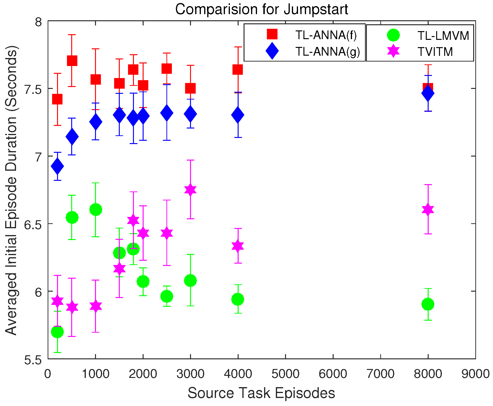
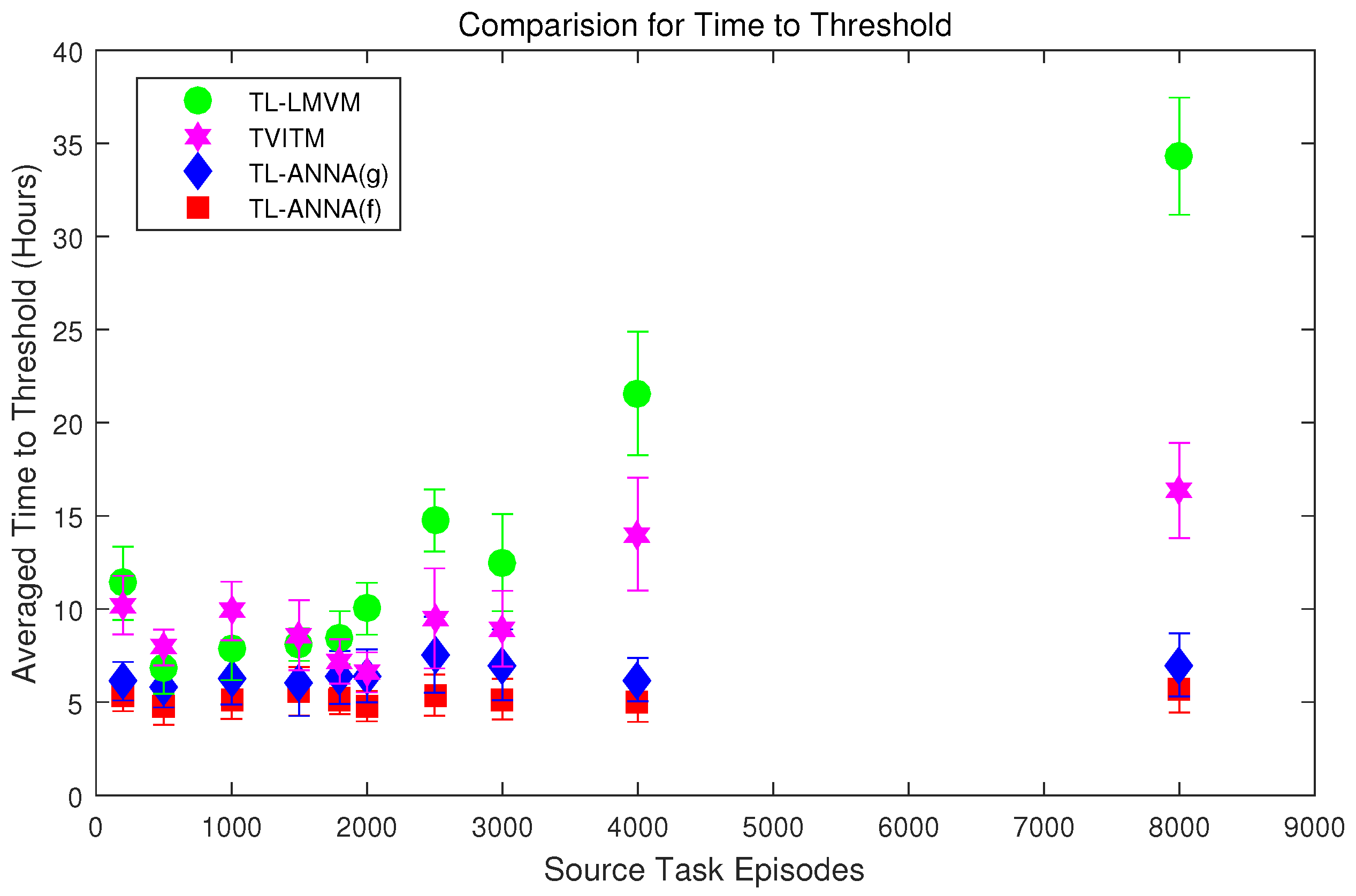
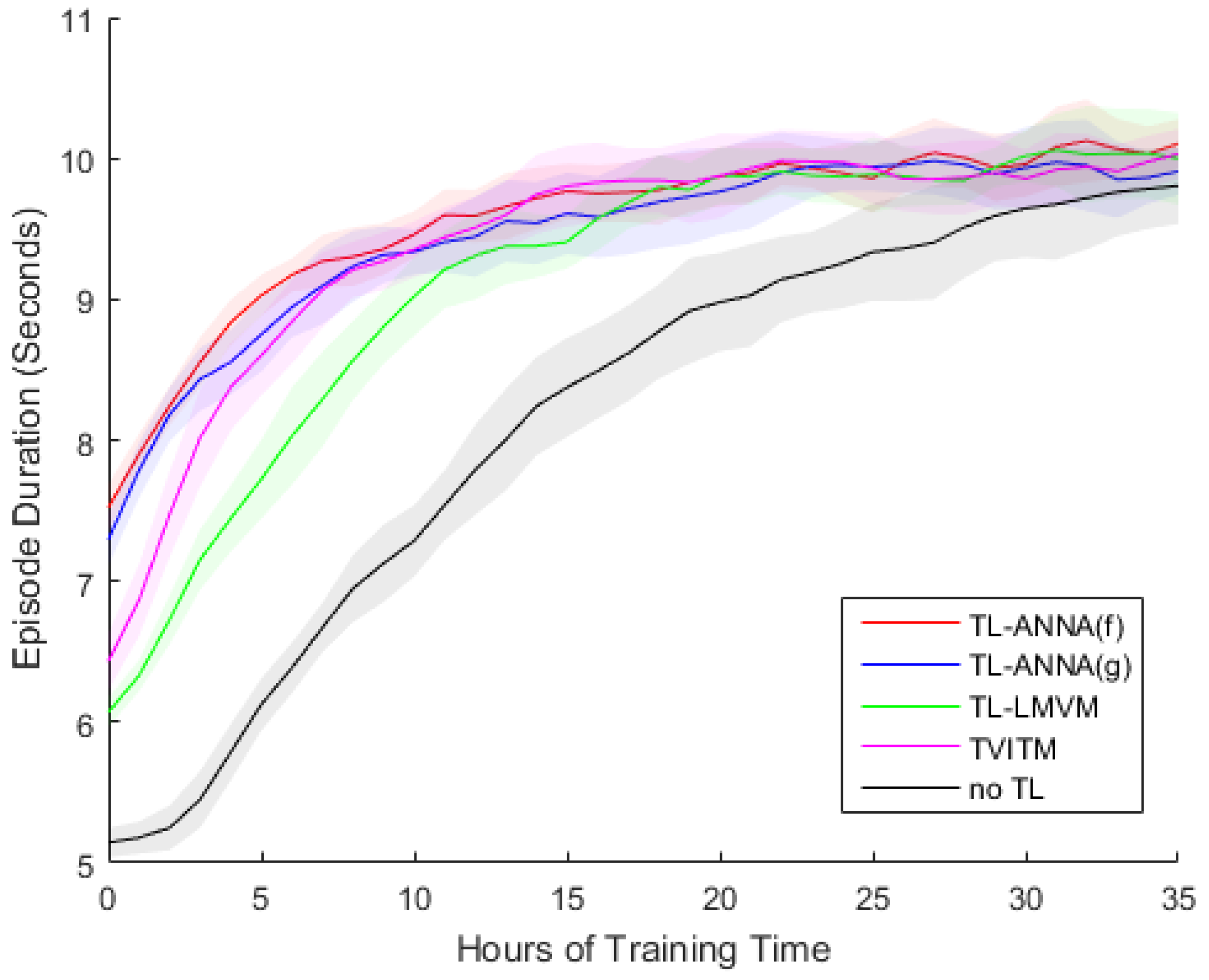
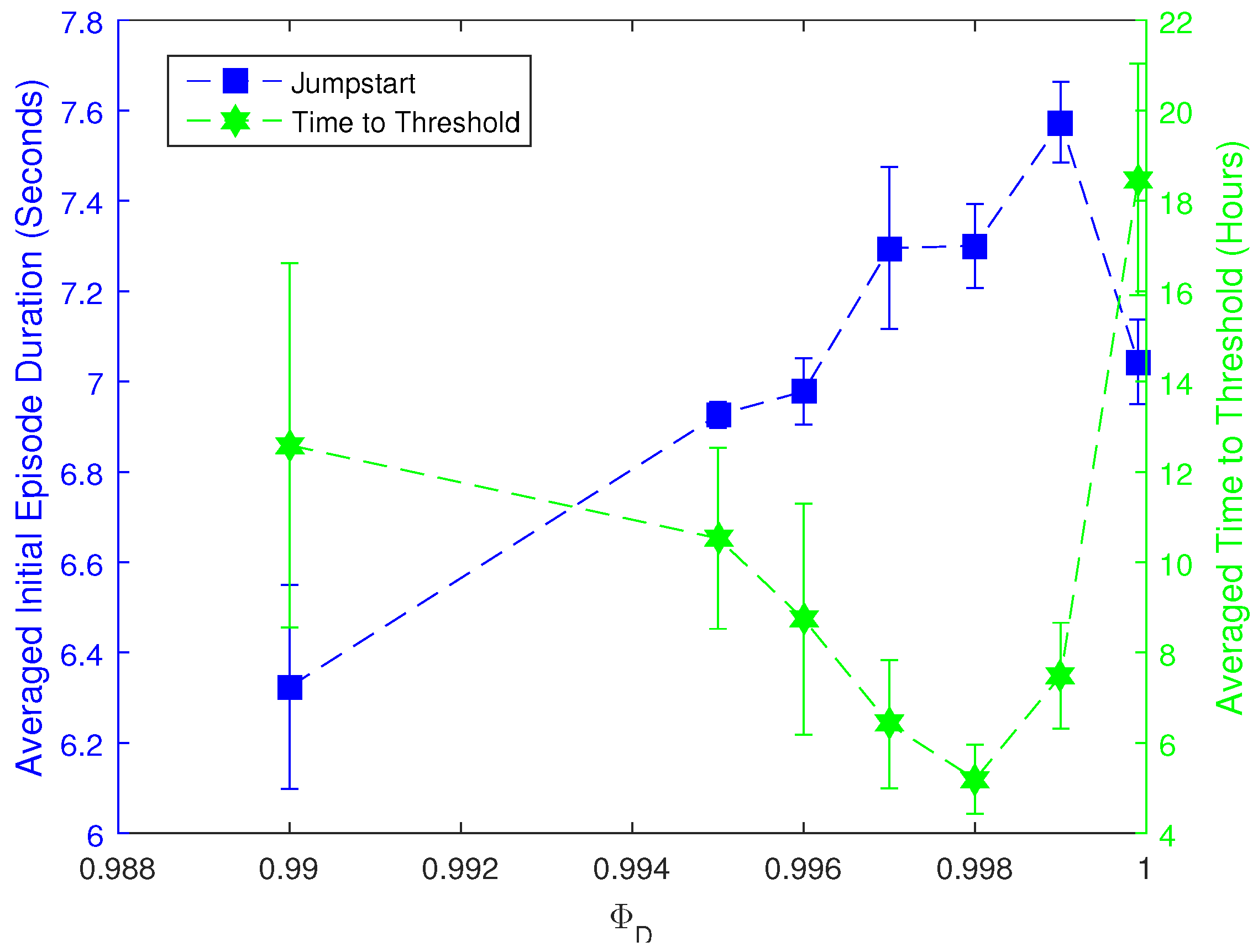
5.3. Experiment Settings and Results

Since there are two types of transfer approximator due to two mapping rules, two sets of experiments have been performed for the proposed TL-ANNA methods. One is with the full mapping rule, and the other is with the group mapping rule. In both sets of experiments, the parameter ${\mathsf{\Phi }}_D$ is set to be 0.997. For comparison, two sets of experiments with two other transfer learning methods have also been performed in the same experimental condition. The first comparison method is Transfer via Inter-Task Mapping (TVITM) [1], and the second one is Transfer via Linear Multi-Variable Mapping (TL-LMVM) [4]. In the TL-LMVM, the variables are grouped before transferring. In this set of experiments for TL-LMVM, the same state variables grouping method as that of the TL-ANNA is used, while the action variables are just grouped into one group. The TL-LMVM method uses the transferred knowledge to initializing the parameters in the target task, where the transferred knowledge for each variable of the target task are the linear combination of the knowledge associated with variables in the corresponding group of the source task. The linear parameters are set with those from [4]. Therefore, there are four sets of experiments in total.

Ten different weight files are collected from the source task after different episodes of learning in it, as stated in Section 5.2. For each source task weight file, four sets of experiments have been run with the above four transfer learning methods, respectively. Each set of experiments is run for 10 trials in the target task, and each trial runs for at least 10,000 episodes. The results of each set of experiments are averaged over these 10 trials.

These proposed methods would bring extra computational complexity in each transferring update due to the use of ANN. However, this extra computational complexity is negligible compared to the sample complexity in reinforcement learning. Thus, the main goal of these proposed methods is to reduce the sample complexity rather than the computational complexity. To measure the effectiveness of transfer learning, many metrics can be used [33]. In this work, two key metrics are used to compare the performance of these four transfer learning methods: jumpstart and the time to threshold.

Jumpstart measures the initial performance that has been improved by transfer learning. Since the episode duration is the performance measure of Keepaway, the initial performance refers to the initial episode duration in these experiments. To reduce errors, the average duration of the first 1000 episodes is calculated as the initial episode duration for comparison. In the 4vs.3 Keepaway learning task without transfer learning, the initial episode duration is $5.14\pm 0.10$ s (averaged over 10 trials). The initial episode duration of all four sets of experiments with different transfer learning methods and different source knowledge are summarized in Figure 3. All the results are averaged over 10 independent trials, and the error bar shows the corresponding averaged initial episode duration and the standard deviation.

In order to gauge the statistically significant difference of the jumpstart metric among the four methods, the Welch’s t-test with $95\%$ confidence is used. Seven sets of Welch’s t-test have been performed: (1) TL-ANNA (full mapping) vs. no transfer; (2) TL-ANNA (group mapping) vs. no transfer; (3) TL-ANNA (full mapping) vs. TL-LMVM; (4) TL-ANNA (group mapping) vs. TL-LMVM; (5) TL-ANNA (full mapping) vs. TVITM; (6) TL-ANNA (group mapping) vs. TVITM; and (7) TL-ANNA (full mapping) vs. TL-ANNA (group mapping). Each set contains 10 Welch’s t-test for there are 10 cases with different source weight files. The first two sets of tests show that both two TL-ANNA methods have significantly longer initial episode duration than the no-transfer learner in all cases, which also indicates no negative transfer occurs. In addition, test sets (3)–(6) show that both two TL-ANNA methods have significantly higher jumpstart than the two comparison methods, TL-LMVM and TVITM, in all cases. That is to say, both proposed methods can set a better start point for the RL learners. Moreover, the last set of Welch’s t-test shows that the TL-ANNA with full mapping has significantly higher jumpstart than the TL-ANNA with group mapping for 9 cases out of all these 10 cases, and only in the case with 8000 episodes of source task learning has no statistical difference. This is probably due to the fact that state features in full mapping can be mapped to all the related source state features. While in the group mapping case, it is hard to group all the related features into the same group very accurately, so the mapping in group mapping may lose part of the related knowledge compared with that of full mapping. Thus, the transfer ability of the group mapping TL-ANNA is slightly weaker than that of the full mapping TL-ANNA in the normal cases. However, the quality of the source task knowledge can also have some influence on the performance of the transfer learning. From Figure 3, it can be seen that the jumpstart of the two comparison methods, TL-LMVM and TVITM, vary a lot by the source task knowledge. In addition, the TL-ANNA with group mapping tends to have higher jumpstart as the learning in the source task set to be longer. While the jumpstarts of the TL-ANNA with full mapping are not influenced too much by the choose of the source task knowledge. This may be the reason for the exception one in the last set of Welch’s t-test results.

Time to threshold measures how fast the learning reaches a threshold with the transfer learning, which can reflect the improvement in reducing the sample complexity. The average episode duration over 1000 episodes reaches about 9.2 s after 30 h of training without transfer learning. Therefore, set the threshold as 9.0 s, and the learning time necessary to reach this threshold is referred as the time to threshold. The learning in the target task is considered to be sufficient when the keepers can maintain an average episode duration of 9.0 s over 1000 episodes. In learning without transfer learning, the average time to reach the threshold of 9.0 s over 10 trials is $20.54\pm 3.88$ h. Figure 4 presents the average time to threshold over 10 trials for each set of transfer learning experiments with different methods and different source task knowledge.

Seven sets of Welch’s t-test are also performed as in the analysis of the jumpstart to detect the significant difference for the time to threshold results among the four different sets of experiments (at the $95\%$ confidence level, each set has 10 tests.). The tests show that both the TL-ANNA with full mapping and the TL-ANNA with group mapping have significantly shorter time to threshold than the learner without transfer in all these 10 cases, which again indicates that no negative transfer occurs in these proposed methods. Moreover, the TL-ANNA with full mapping reaches the threshold in a significantly shorter time than both the TL-LMVM and the TVITM do in all cases. The TL-ANNA with group mapping reaches the threshold in a significantly shorter time than the TL-LMVM does in all cases, while it has significantly shorter time to threshold than the TVITM in eight cases, and has no statistical difference only in the two cases with 1800 episodes and 2000 episodes of source task learning. The TL-ANNA with full mapping reaches the threshold significantly faster than the TL-ANNA with group mapping in nine cases, and only the case with 1500 episodes of source task learning has no statistical difference. From Figure 4, it can be noticed again that both the TL-LMVM and the TVITM are influenced by the quality of the source task knowledge very much, while both two TL-ANNA methods are more robust to the quality of the source task knowledge, especially the TL-ANNA with full mapping.

Among so many tested cases, only one or two cases can not tell the significant difference between these proposed methods and the comparison methods. Therefore, these proposed TL methods can be generally regarded as better than the other two TL methods, and the TL-ANNA with full mapping is better than the TL-ANNA with group mapping. However, both the results presented in Figure 3 and Figure 4 have not considered the time required for collecting samples in the target task and the time required for training the ANNs. In our case, the time for collecting samples is in minutes, and the time for training the ANNs (Table 3) is either in seconds (for group mapping case) or in minutes (for full mapping case), while the time shortened by TL-ANNA is in hours. Therefore, it can be considered that the time needed for preparing the transfer learning can be ignored, whereas, even if there are cases where the time needed before the transfer learning is close to the time been shorten by the transfer learning, there is still benefit from the TL-ANNA that the TL-ANNA removes the need of the action mapping and even reduce the human involvement with certain state feature mapping rule. However, for tasks that have totally dissimilar action sets, the effects of the TL-ANNA have not been tested yet, therefore good performance can not be guaranteed in such cases. Furthermore, the TL-ANNA methods are more robust to the quality of the source knowledge, which can reduce the time spent on the selection of the source knowledge. On the other hand, the robustness to the quality of the source knowledge also means that the proposed methods are more robust to the negative transfer, though it is hard to guarantee that there will be no negative transfer when transfer between two unrelated tasks. Therefore, attention still needs to be paid on the selection of the source task to avoid negative transfer, but less energy can be paid on selecting the quality of the source knowledge. In addition, the full mapping TL-ANNA works slightly better than the group mapping TL-ANNA, possibly due to the fact that more source knowledge can be conserved in the full mapping case than the group mapping case. However, the full mapping case costs much more in terms of computation and space than the group mapping one, including in the training for the ANNs. Usually, the reducing of the computation and space in the TL-ANNA with the group mapping comes in the price of extra computation for grouping with methods like clustering or extra human involvement in the grouping.

Another thing needs to be noted is that there are some errors brought into the ANNs by the roughly determined training data. However, the experimental results show that such errors do not effect too much of the effectiveness of the proposed methods. As for to what extent that the proposed transfer learning framework can tolerate the errors from the ANNs, it is still not sure and can be left for future work. In cases that the training data are accurately determined to reflect the relationship between the source task and the target task, more training time for the ANNs can be expected to be more beneficial for the performance of the transfer learning, such as reducing more time for the reinforcement learning in the target task. However, too much training time for the ANNs could add up more time to the whole learning process, which makes the time shorten by the transfer learning appear to be not that much worthwhile. Since the proposed methods are affected more by the quality of the source task than by the errors in the ANNs, it is not recommended to spend too much time on training the ANNs.

To show the difference of the learning process with different transfer learning methods in more detail, Figure 5 illustrates the learning process for one of these ten groups of experiments. The source task knowledge for this group of experiments is collected after learning for 2000 episodes in the 3vs.2 Keepaway task.

Finally, a set of experiments are also performed to test the effect of the parameter ${\mathsf{\Phi }}_D$ in the proposed transfer learning methods. This set of experiments uses the group mapping TL-ANNA method to transfer from 3vs.2 Keepaway to 4vs.3 Keepaway with different values of ${\mathsf{\Phi }}_D$, and all the runs use the source task weight file obtained after learning for 2000 episodes in the 3vs.2 Keepaway. Six extra different ${\mathsf{\Phi }}_D$ values ranging from 0.99 to 0.9999 are tested (initial experiments show that the transfer learning performance is much worse when ${\mathsf{\Phi }}_D\le 0.9$), and the experiments for each ${\mathsf{\Phi }}_D$ value are run for four trials. The initial episode duration and the time to threshold (also a threshold of 9.0 s) for each group of experiments with different ${\mathsf{\Phi }}_D$ values are presented in Figure 6, where each result is averaged over four trials, except that results for ${\mathsf{\Phi }}_D=0.9970$ are averaged over 10 trials.

As shown by Figure 6, the parameter ${\mathsf{\Phi }}_D$ does have a great deal of influence on the performance of transfer learning. Approximately, the bigger the ${\mathsf{\Phi }}_D$ is, the more likely this transfer learning can help the RL learner acquire a longer initial episode duration and reach the threshold in a shorter time. However, as the ${\mathsf{\Phi }}_D$ approaches 1, the effects would turn worse. In short, the choice of ${\mathsf{\Phi }}_D$ should be big enough but not too close to 1.

6. Conclusions

In this work, a new transfer learning framework has been proposed to transfer knowledge from the source task to the target task with a transfer approximator and the PPR scheme. The transfer approximator can use full mapping or group mapping to map the state in the target task into the source task. Through the ANNs, the transfer approximator can suggest a transferred action to bias the learning in the target task, where the transferred action is a target task action, so no action mapping is needed in this framework. With a good deal of experiments performed on the Keepaway task, it has been verified that the proposed TL-ANNA methods outperform the other two transfer learning methods, TL-LMVM and TVITM. In addition, the TL-ANNA with full mapping usually works slightly better than the TL-ANNA with group mapping, and the fact that full mapping is totally task independent makes the TL-ANNA with full mapping more promising. However, the TL-ANNA with full mapping costs more in terms of computation and space, particularly in tasks with too many state features. Though less computation and space consumption, the TL-ANNA with group mapping may require extra computation from grouping methods like clustering or extra human involvement in grouping. Therefore, users should balance the two methods based on their requirements and task properties. In addition, the performance of TL-ANNA is very robust to the quality of source knowledge, while other transfer learning methods seldom have this property. However, the proposed TL-ANNA can be influenced by the parameter ${\mathsf{\Phi }}_D$. By following the strategy given in this paper when choosing the value for ${\mathsf{\Phi }}_D$, the performance of TL-ANNA can avoid being worsened by the parameter ${\mathsf{\Phi }}_D$.

However, there are still many aspects that can be explored in future works. First, other forms of the state feature mapping rules for the transfer approximator may exist. Second, the grouping method such as clustering could be explored, so as to make the group mapping rule less human involved. Third, other methods to generate the training data or even more accurate output samples for the ANNs may be worth being explored to improve the performance of the proposed transfer learning methods. Fourth, methods for finding a more suitable number of hidden nodes in the ANNs and achieving a better performance of the ANNs could be explored. Fifth, the BP ANNs could also be replaced by other forms of ANNs or even other supervised learning methods. Sixth, more layers of ANNs and even deep learning techniques could be applied to test the performance of the proposed framework. Seventh, other methods to combine with the PPR scheme could be studied. Eighth, methods that can reduce the computational complexity could be examined in the future. Lastly, other schemes to reuse the transferred action could be explored.

References

1. Taylor, M.E.; Stone, P.; Liu, Y. Transfer learning via inter-task mappings for temporal difference learning. J. Mach. Learn. Res. 2007, 8, 2125–2167. [Google Scholar]
2. Fernández, F.; Veloso, M. Probabilistic Policy Reuse in a Reinforcement Learning Agent. In Proceedings of the Fifth International Joint Conference on Autonomous Agents and Multiagent Systems, Hakodate, Japan, 8–12 May 2006. [Google Scholar]
3. Taylor, M.E.; Suay, H.B.; Chernova, S. Integrating reinforcement learning with human demonstrations of varying ability. In Proceedings of the 10th International Conference on Autonomous Agents and Multiagent Systems, Taipei, Taiwan, 2–6 May 2011; pp. 617–624. [Google Scholar]
4. Cheng, Q.; Wang, X.; Shen, L. Transfer learning via linear multi-variable mapping under reinforcement learning framework. In Proceedings of the 2017 36th Chinese Control Conference (CCC), Dalian, China, 26–28 July 2017; pp. 8795–8799. [Google Scholar]
5. Taylor, M.E.; Kuhlmann, G.; Stone, P. Autonomous transfer for reinforcement learning. In Proceedings of the Seventh International Joint Conference on Autonomous Agents and Multiagent Systems, Estoril, Portugal, 12–16 May 2008. [Google Scholar]
6. da Silva, F.L.; Costa, A.H.R. Towards Zero-Shot Autonomous Inter-Task Mapping through Object-Oriented Task Description. In Proceedings of the Transfer in Reinforcement Learning Workshop (TiRL) in AAMAS 2017, São Paulo, Brazil, 8–12 May 2017; pp. 1–10. [Google Scholar]
7. Cheng, Q.; Wang, X.; Shen, L. An Autonomous Inter-task Mapping Learning Method via Artificial Neural Network for Transfer Learning. In Proceedings of the 2017 IEEE International Conference on Robotics and Biomimetics, Macao, China, 5–8 December 2017; pp. 768–773. [Google Scholar]
8. Wang, Z.; Taylor, M.E. Effective Transfer via Demonstrations in Reinforcement Learning: A Preliminary Study. In Proceedings of the 2016 AAAI Spring Symposium Series, Palo Alto, CA, USA, 21–23 March 2016; The AAAI Press: Palo Alto, CA, USA, 2016. [Google Scholar]
9. Brys, T.; Harutyunyan, A.; Taylor, M.E.; Nowé, A. Policy transfer using reward shaping. In Proceedings of the 2015 International Conference on Autonomous Agents and Multiagent Systems, Istanbul, Turkey, 4–8 May 2015; International Foundation for Autonomous Agents and Multiagent Systems: Richland, SC, USA, 2015; pp. 181–188. [Google Scholar]
10. Du, Z.; Wang, C.; Sun, Y.; Wu, G. Context-Aware Indoor VLC/RF Heterogeneous Network Selection: Reinforcement Learning with Knowledge Transfer. IEEE Access 2018, 6, 33275–33284. [Google Scholar] [CrossRef]
11. Zhan, Y.; Taylor, M.E. Online transfer learning in reinforcement learning domains. arXiv, 2015; arXiv:1507.00436. [Google Scholar]
12. Koga, M.L.; Freire, V.; Costa, A.H. Stochastic abstract policies: Generalizing knowledge to improve reinforcement learning. IEEE Trans. Cybern. 2015, 45, 77–88. [Google Scholar] [CrossRef] [PubMed]
13. Laflamme, S. Transfer in Reinforcement Learning: An Empirical Comparison of Methods in Mario AI. Master’s Thesis, McGill University Libraries, Montreal, QC, Canada, 2017. [Google Scholar]
14. Laroche, R.; Barlier, M. Transfer Reinforcement Learning with Shared Dynamics. In Proceedings of the AAAI-17—Thirty-First AAAI Conference on Artificial Intelligence, San Francisco, CA, USA, 4–9 February 2017; pp. 2147–2153. [Google Scholar]
15. Wang, Y.; Meng, Q.; Cheng, W.; Liug, Y.; Ma, Z.M.; Liu, T.Y. Target Transfer Q-Learning and Its Convergence Analysis. arXiv, 2018; arXiv:1809.08923. [Google Scholar]
16. Faudzi, A.A.M.; Takano, H.; Murata, J. Transfer Learning Through Policy Abstraction Using Learning Vector Quantization. J. Telecommun. Electron. Comput. Eng. 2018, 10, 163–168. [Google Scholar]
17. Matsubara, T.; Norinaga, Y.; Ozawa, Y.; Cui, Y. Policy Transfer from Simulations to Real World by Transfer Component Analysis. In Proceedings of the 14th IEEE International Conference on Automation Science and Engineering, Munich, Germany, 20–24 August 2018. [Google Scholar]
18. Schwab, D.; Zhu, Y.; Veloso, M. Zero Shot Transfer Learning for Robot Soccer. In Proceedings of the 17th International Conference on Autonomous Agents and MultiAgent Systems, Stockholm, Sweden, 10–15 July 2018; International Foundation for Autonomous Agents and Multiagent Systems: Richland, SC, USA, 2018; pp. 2070–2072. [Google Scholar]
19. Gupta, A.; Devin, C.; Liu, Y.; Abbeel, P.; Levine, S. Learning invariant feature spaces to transfer skills with reinforcement learning. arXiv, 2017; arXiv:1703.02949. [Google Scholar]
20. Lehnert, L.; Tellex, S.; Littman, M.L. Advantages and Limitations of using Successor Features for Transfer in Reinforcement Learning. arXiv, 2017; arXiv:1708.00102. [Google Scholar]
21. Shoeleh, F.; Asadpour, M. Graph based skill acquisition and transfer learning for continuous reinforcement learning domains. Pattern Recognit. Lett. 2017, 87, 104–116. [Google Scholar] [CrossRef]
22. Joshi, G.; Chowdhary, G. Cross-Domain Transfer in Reinforcement Learning using Target Apprentice. arXiv, 2018; arXiv:1801.06920. [Google Scholar]
23. Kelly, S.; Heywood, M.I. Knowledge Transfer from Keepaway Soccer to Half-field Offense through Program Symbiosis: Building Simple Programs for a Complex Task. In Proceedings of the 2015 Annual Conference on Genetic and Evolutionary Computation, Madrid, Spain, 11–15 July 2015; ACM: New York, NY, USA, 2015; pp. 1143–1150. [Google Scholar]
24. Didi, S.; Nitschke, G. Multi-agent behavior-based policy transfer. In Proceedings of the 19th European Conference on the Applications of Evolutionary Computation, Porto, Portugal, 30 March–1 April 2016; Springer: Berlin/Heidelberg, Germany, 2016; pp. 181–197. [Google Scholar]
25. Rajendran, J.; Prasanna, P.; Ravindran, B.; Khapra, M. Adaapt: A deep architecture for adaptive policy transfer from multiple sources. arXiv, 2015; arXiv:1510.02879. [Google Scholar]
26. Sutton, R.S.; Barto, A.G. Reinforcement Learning: An Introduction; MIT Press: Cambridge, UK, 1998. [Google Scholar]
27. Albus, J.S. Brains, Behaviour, and Robotics; Byte Books: Perterborough, NH, USA, 1981. [Google Scholar]
28. Chung, I.H.; Sainath, T.N.; Ramabhadran, B.; Picheny, M.; Gunnels, J.; Austel, V.; Chauhari, U.; Kingsbury, B. Parallel deep neural network training for big data on blue gene/q. IEEE Trans. Parallel Distrib. Syst. 2017, 28, 1703–1714. [Google Scholar] [CrossRef]
29. Połap, D.; Woźniak, M.; Wei, W.; Damaševičius, R. Multi-threaded learning control mechanism for neural networks. Future Gener. Comput. Syst. 2018, 87, 16–34. [Google Scholar] [CrossRef]
30. Fernández, F.; García, J.; Veloso, M. Probabilistic policy reuse for inter-task transfer learning. Robot. Auton. Syst. 2010, 58, 866–871. [Google Scholar] [CrossRef]
31. Shi, H.; Lin, Z.; Hwang, K.S.; Yang, S.; Chen, J. An Adaptive Strategy Selection Method With Reinforcement Learning for Robotic Soccer Games. IEEE Access 2018, 6, 8376–8386. [Google Scholar] [CrossRef]
32. Stone, P.; Kuhlmann, G.; Taylor, M.E.; Liu, Y. Keepaway soccer: From machine learning testbed to benchmark. In Robot Soccer World Cup; Springer: Berlin/Heidelberg, Germany, 2005; pp. 93–105. [Google Scholar]
33. Taylor, M.E.; Stone, P. Transfer learning for reinforcement learning domains: A survey. J. Mach. Learn. Res. 2009, 10, 1633–1685. [Google Scholar]
Figure 1. The proposed TL (Transfer Learning) framework with ANN (Artificial Neural Network) transfer approximator.
Symmetry 11 00025 g001
Figure 2. The comparison between two TL ideas and no-transfer RL (Reinforcement Learning).
Symmetry 11 00025 g002
Figure 3. The comparisons for jumpstart among the four transfer learning methods. The error bars show the averaged initial episode duration over 10 trials and their standard deviations when using different source knowledge and transfer learning methods. The source knowledge is collected in the 3vs.2 Keepaway after different episodes of learning.
Symmetry 11 00025 g003
Figure 4. The comparisons for time to threshold among the four transfer learning methods. The threshold is set to be 9.0 s of episode duration. The error bars show the averaged time to this threshold over 10 trials and their standard deviations when using different source knowledge and transfer learning methods. The source knowledge is collected in the 3vs.2 Keepaway after different episodes of learning.
Symmetry 11 00025 g004
Figure 5. The learning process for four TL methods and the no-TL learning. The source task knowledge is obtained after learning for 2000 episodes in the 3vs.2 Keepaway. Each line is averaged over 10 trials, and the shadow indicates the standard variation.
Symmetry 11 00025 g005
Figure 6. The comparisons for the effect of different Φ D values. The blue line denotes the averaged initial episode duration (Jumpstart). The green line presents the time to threshold. All values are averaged over four trials, except that the values for Φ D = 0.997 are averaged over 10 trials. The error bars also indicate the corresponding standard deviations. The TL method used is TL-ANNA with group mapping, and the source knowledge is collected in the 3vs.2 Keepaway after 2000 episodes of learning.
Symmetry 11 00025 g006