Abstract
Pixel value ordering (PVO) hiding scheme is a kind of data embedding technique that hides a secret message in the difference of the largest and second largest pixels of a block. After that, the scholars improved PVO scheme by using a threshold to determine whether the block is smooth or complex. Only a smooth block can be used to hide information. The researchers analyzed all the possible thresholds to find the proper one for hiding secret message. However, it is time consuming. Some researchers decomposing the smooth block into four smaller blocks for hiding more messages to increase image quality. However, the complexity of the block is more important than block size. Hence, this study proposes an ameliorated method. The proposed scheme analyzes the variation of the region so as to judge the complexity of the block and applies quantification strategy to quantified the pixel for making sure the pixel is reversible. It adopts an adaptive threshold generation mechanism to find the proper threshold for different images. The results show that the image quality of the proposed scheme is higher than that of the other methods. The proposed scheme can also let the user adjust the hiding rate to achieve higher image quality or hiding capacity.
1. Introduction
Reversible Data Hiding (RDH) is a kind of technique used to extract embedded confidential information from image media, and restore the image back to its most primitive state [1]. Based on hiding methods, the RDH technique can be divided into two main types. First the histogram displacement method pointed out by Ni et al. [2]. This method employs statistics of pixel values or prediction of error value distribution, finds out frequently appearing items and consider them peak value points, and items which has not appeared before are considered as zero value points. The items located between peak value points and zero value points will be shifted to the next position; and the peak value points will be treated as positions with embedded confidential information. Another method is Tian’s difference expansion technique. This method utilizes the difference between pixels, or the difference between pixels and predicted values, to perform expansion in multiples and embeds confidential information in the difference values after expansion [3,4]. The main research directions of the current RDH techniques focused mainly on how to enhance the overall hiding capacity and how to enhance the image quality [5].
To enhance the hiding capability, many scholars used predictors in combination with RDH technique. The confidential information is embedded using the predicted errors generated by the original pixel values and predicted values. The more accurate the predicted values, the smaller the errors, and the larger the hiding capacity. For instance, Thodi and Rodriguez [6], Luo et al. [7], and Hong et al. [8] modified Weinberger’s edge Median Edge Detection (MED) to increase the information hiding capacity. MED uses three adjacent pixel values for prediction. One of these adjacent pixels will be the base pixel, and together with the other two pixels, a degree of complexity is computed, and then the predicted pixel is generated. Fallahpour [9], Coltuc [10] and Li et al. [11] used Wu’s and Memon’s Gradient Adjusted Prediction (GAP) to enhance prediction accuracy of edge pixels. GAP uses seven adjacent pixel values for prediction, performs tests on horizontal edges and vertical edges to compute correlation coefficients which are either strong or weak. In this way it is able to more accurately predict edge blocks [12]. Lu [13], Feng and Fan [14] used Lukac’s edge sensitivity predictor and extended its application. In this method the sensitive coefficients of adjacent pixels are computed and then normalized to weights. The weights and original pixels are then multiplied and the resultant values are added to form the predicted pixel value [15].
Recently, to improve the accuracy of prediction, Li et al. proposed a new RDH prediction method in 2013. It is called the Pixel Value Ordering (PVO) strategy [16,17,18]. In this method pixel values in the same set are first sorted out in ascending order. After that the two largest pixels are used to compute the maximum difference value, and the 2 smallest pixels are used to compute the minimum difference. Lastly, the confidential information is hidden into the maximum and minimum pixels. This method uses the sorted results to generate predicted errors. It effectively reduces the gap in the difference, and does not affect the sorted results while modifying the pixel values so that the pixel values can be restored to the original states. In 2014, Peng et al. proposed the modified PVO prediction method [19]. To enhance hiding capability, after sorting the pixel values, the index sequence was used to generate predictive errors of positive and negative values. Further, a bimodal histogram displacement technique was designed for embedding. For example, let represent a sorted set. Two maximum values are 10 and 9. The maximum difference is 10 – 9 = 1. The two minimum values are 3 and 4. The minimum difference is 3 − 4 = −1. If the maximum difference is equal to 1 then the value is embeddable. At the same time, if the minimum difference is equal to −1, then the pixel is embeddable. In this case, both the maximum difference and the minimum difference are embeddable. Hence, the hiding capacity is twice of the original hiding scheme.
Wang modified Peng’s method in 2015. He used the complexity of a set to determine the capacity of confidential information hiding. Image distortion was also reduced [19,20,21]. For example, assume the set is . The complexity of the set is very large such that cannot be used conceal information. In PVO scheme, the maximum value 254 and the minimum value 5 will be respectively shifted to 255 and 4 for further recovering. The shifting will make a great image distortion.
The method proposed by Peng et al. uses a threshold value to determine whether the region is smooth or complex. Only smooth regions may be used to hide confidential information. For example, in Peng et al.’s scheme, the complexity of the set is larger than the threshold. Hence, the set is skipped without doing any embedding or shifting to keep high image quality.
However, the setting of threshold value did not have an effective mechanism. Peng et al. employed a rather crude approach. The test will start from value 1 until the maximum tolerable value is attained. An acceptable threshold value is then picked from this value range. This approach is not ideal and it is also time consuming. Besides, this method may also have an overflow problem. This study is designed to improve Peng’s proposed method. Variability of the block itself is used to determine whether the block can be used for hiding. To ensure that the recipient can obtain the same variance, the proposed method will conduct quantization of the block. Even if the quantized value has hidden message, the recipient can re-quantize the camouflaged pixel and still obtain the same quantized value. Besides, how to determine the threshold value is another issue. This study employs the self-adaptive threshold value setting method. The proper threshold value is derived via analyzing the variability, and is used enhance the image quality.
2. Related Works
In 2013, Li et al. proposed a pixel value sequencing strategy to enhance the overall image quality. It is combined with the prediction error expansion (PEE) technique for information embedding [18]. Figure 1 shows that how Li et al.’s method works. First of all, the method divides the image into many blocks of the same size. Each block is represented by a set. Let represent the set. Within the set, there are n pixels in total. The pixel values in each set are sorted in ascending order, ; where is the index position after sorting. Pixel values will be sorted in a sequence based on , … .
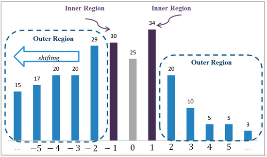
Figure 1.
Li et al.’s PVO Difference Histogram.
Next, the maximum predicted error is generated through using the difference between the largest pixel value and the second largest pixel value . Similarly, the minimum predicted error is generated through using the difference between the smallest pixel value and the second smallest pixel value . The equations are shown as follows:
In the embedding stage, Li et al. divided the histogram into two parts, left-hand side part and right-hand side part. Each part separated into two regions, Inner Region and Outer Region. If the error values are located in 1 and −1, the values were in the Inner Region. Otherwise, the values are located in the Outer Region. Figure 1 demonstrates an example.
In Li’s experiments, it was found that when the predicted difference values and generated by PVO were used, the peak value points of most images would fall within 1 and −1. To maintain image quality, the error value 0 was excluded, without doing any embedding and displacement. The error values 1 and −1 were deemed as the Inner Region where confidential information can be embedded. The remaining error values were deemed as Outer Region and displacement were performed. If the predicted difference value is equal to 1, then one secret bit b can be concealed into the value to generate the stego-value . If is equal to 0, then the value cannot be used to hide information and the stego-value is equal to its original value . Otherwise, does not located in the inner region and is not equal to 0, then the value needs to be shifted by +1. On the other side, if the predicted difference value is equal to −1, then one secret bit b can be concealed into the value to generate the stego-value . If is equal to 0, then the value cannot be used to hide information, then the stego-value is equal to its original value . If does not located in the inner region and is not equal to 0, then the value needs to be shifted by 1.
The embedding equations were as follows:
Figure 2 is taken as an example. The image is first cut into many blocks. In this example, four pixels are grouped as a set. The pixel value combination of the first set is X = {5, 4, 15, 19}. After sorting in ascending order, the = {4, 5, 15, 19} is obtained. Through Equation (1), the derived values are the maximum predicted error = 19 − 15 = 4 and the minimum predicted error = 4 − 5 = −1. In this case, = 4 is located in the Outer Region. Through Equation (2), displacement is conducted on original pixels and a camouflaged pixel value = 19 + 1 = 20 is generated; and = −1 falls in the Inner Region. Through Equation (3), the embedded confidential information is s = 1; and it generates a camouflaged pixel value = 4 − 1 = 3.
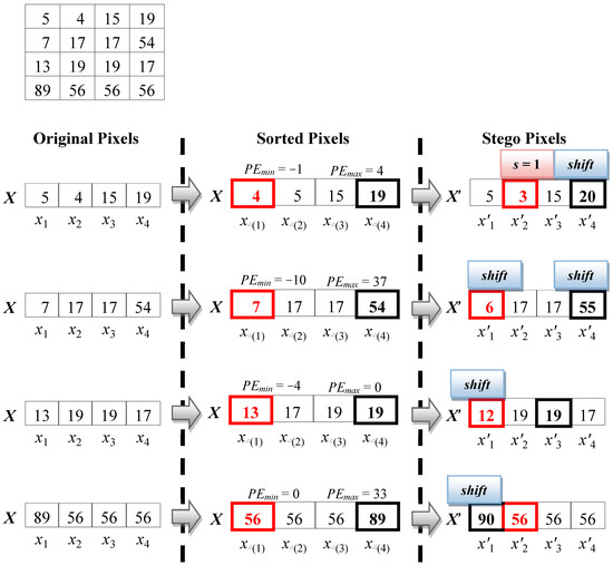
Figure 2.
Li et al.’s PVO Embedding Example.
The PVO technique proposed by Li et al. first sorts the pixel values in the same block in ascending order. Then it uses the difference between the largest pixel and the second largest pixel as the error value (or the error value between the smallest pixel and the second smallest pixel). Finally, the maximum pixel values are modified in ascending way and the minimum pixel values are modified in descending way, so that the predicted errors are reduced and they also keep the original sorted sequence. However, their approach ignores the position where the error is 0. From Figure 1, it can be found that error value 0 is the second most frequently occurring position. It should be noted that Li et al. did not effectively use the error value.
Peng et al. expanded the PVO method of Li et al. to Improved Pixel-Value-Ordering (IPVO) method. They adopted the bimodal strategy to expand the embedded confidential information in Inner Region to errors of ±1 and 0 [16]. They modified the method by which the predicted value for predicted errors and is generated so that the maximum pixel value and minimum pixel value would not affect the sorting result. The maximum error value could also produce a negative error value for the left shift displacement of error value 0; and the minimum error value could also produce a positive error value for the right shift displacement of error value 0. As shown in Figure 3, Figure 3a is the maximum error histogram maximum predicted error and Figure 3b is the minimum error histogram maximum predicted error. The equations for predicted errors and are shown as follows:
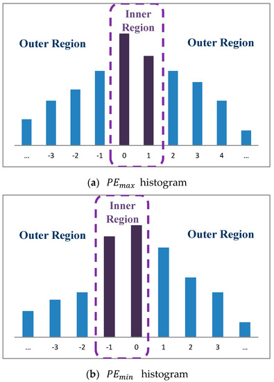
Figure 3.
The PVO Difference Histogram of Peng et al.
Supposing that u and v are the largest pixel index value and the second largest pixel index value after sorting; s and t were the smallest pixel index value and second smallest pixel index value after sorting, Peng et al. use the index values u, v, s, and t to produce positive and negative predicted errors. Take for an example a pixel set X = {12, 17, 2, 1}. After sorting, it becomes = {1, 2, 12, 17}. The sorted index value pairs are, in order, Δ(1) = 4, Δ(2) = 3, Δ(3) = 1, and Δ(4) = 2. Through Equation (4), it comes to u = min(1, 2) = 1 and v = max(1, 2) = 2. Finally, the maximum predicted error is = 12 − 17 = −5. Similarly, through Equation (5), it derives s = min(4, 3) = 3 and t = max(4, 3) = 4. Finally, minimum predicted error is = 2 − 1 = 1.
Peng et al. then modified the embedding and displacing Equations (2) and (3) to Equations (4) and (5), embedding confidential information into the Inner Region and displacing other pixel values in the Outer Region. The relevant embedded equations are as follows:
Figure 4 is an example to explain the equations. The pixel value set of first block is X = {5, 4, 15, 19}. After sorting in ascending order, it becomes = {4, 5, 15, 19}. The respective index values are Δ(1) = 2, Δ(2) = 1, Δ(3) = 3, and Δ(4) = 4. Through Equations (4) and (5), the derived maximum predicted error is = 15 − 19 = −4; and the minimum predicted error is = 5 − 4 = 1. = −4 falls in Outer Region. Through Equation (6), displacement is conducted on original pixels, and a camouflaged pixel value Δ(4) = 19 + 1 = 20 is generated. = 1 also falls on Outer Region. Through Equation (7), camouflaged pixel value = 4 − 1 = 3 is generated.
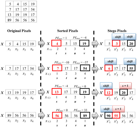
Figure 4.
The PVO Embedding Example of Peng et al.
Through using the sequence order of index positions, Peng et al. made the error values and capable of having corresponding positive and negative errors, and thus the two histograms can effectively use the error value 0 for bimodal displacement. The method also effectively enhanced the overall hiding capability. However, through this method, the maximum pixel value and minimum pixel value are all displaced in each block, resulting in severe image distortion.
In 2015, Wang et al. proposed the modified Peng’s PVO method. The method goes as follows. An image is divided into 4 × 4 fixed size blocks. Then the complexity of the blocks is determined through threshold values T1 and T2. In this way, the displacement extent of high complexity blocks can be reduced, and hence image quality is enhanced [20]. First, the image is cut into many blocks 4 × 4 in size. Further, the pixels in each block are divided into four sets of sub-blocks 4 × 4 in size and sorted in ascending order. Next, in each block, complexity computation is using the second smallest pixel value and the second largest pixel value . The equation for complexity computation is as follows:
Let NL be the difference extent of the block. Pixel values , ), , and are the second largest pixel values in the four sub-blocks. Pixel values , , , and are the second smallest pixel values in the four sub-blocks. Take Figure 5b as an example. Through Equation (8), we know that the complexity of the large block is NL = max(7, 19, 56, 56) − min(5, 17, 19, 19) = 56 − 5 = 51. The computation flow is shown in Figure 5.
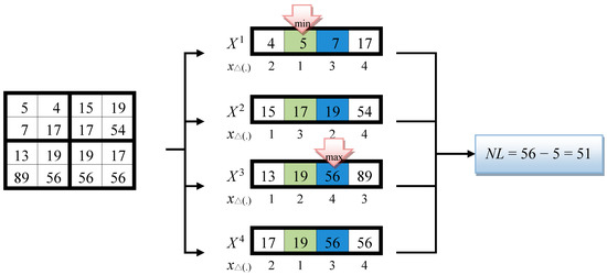
Figure 5.
Wang’s Computation of PVO Block Complexity.
Next, the two thresholds T1 and T2 are used to judge the block complexity, and the threshold values are between –1 T2 T1 255. Blocks of different complexity are processed as either one of the following three Cases to process:
- Case 1: When NL > T1, it indicates that the block is a high complexity area. There will not be any message embedding and displacement.
- Case 2: When T2 < NL T1, it indicates that the block is a common complex area. Since the block is not smooth, the errors generated in the four blocks will mostly fall in the Outer Region; their displacements cannot increase the hiding capacity and may even lead to image distortion; Hence the 4 × 4 block is sorted directly and Peng’s method is used to generate error values, and confidential information embedding and pixels displacement are performed.
- Case 3: When NL T2, it indicates that the block is a smooth block, and embedding and displacement may be performed on each of the four sub-blocks individually; hence they are sorted in 2 × 2 blocks. Peng’s method is used for embedding.
Figure 6 is used as an example. It is assumed that the threshold values are T2 = 15 and T1 = 60. When the four sub-block pixel combination in the first 4 × 4 block is = {5, 4, 7, 17}, = {15, 19, 17, 54}, = {13, 19, 89, 56}, and = {19, 17, 56, 56}, and each sub-blocks are sorted individually; through Equation (8), the computed block complexity is NL = max(7, 19, 56, 56) − min(5, 17, 19, 19) = 51. When T2 < NL T1, it conforms to the general complexity block in Case 2, hence the entire block is reordered. Using Equations (4) and (5) the computed maximum error value = 89 − 56 = 33 and the minimum error value = 5 − 4 = 1. Finally, Equations (6) and (7) are used to generate the camouflaged pixel values = 89 + 1 = 90 and = 4 − 1 = 3. When the four sub-block pixel combination in the second block are = {19, 17, 20, 21}, = {15, 14, 14, 18}, = {22, 22, 20, 24}, and = {16, 14, 10, 12}, sort each sub-block individually and use Equation (8) to compute the block complexity NL = max(20, 15, 22, 14) − min(19, 14, 22, 12) = 10. When NL T2, it conforms to the smooth block in Case 3. Therefore, embedding and displacement will be conducted in each sub-block individually. Take = {14, 14, 15, 18} as an instance. Through Equations (4) and (5), the computed error values are = −3 and = 0. Finally, using Equations (6) and (7), the confidential information s = 0 is embedded and displaced to give = 18 + 1 = 19 and = 14 − 0 = 14. The camouflaged pixel values of the four sub-blocks can be obtained in the same way.
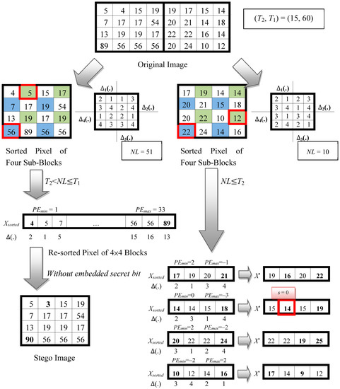
Figure 6.
PVO embedded example of Wang et al.
Wang et al. employed the sorted pixel values and to compute the block complexity NL, and used the threshold values to determine the Case where the block complexity fits. The logic goes as follows. When NL > T1, it means that the block complexity is high, the computed difference values and , will not fall in the Inner Region where embedding may be performed and instead fall in the Outer Region, resulting in pixel value modification and hence serious image distortion. When T2 < NL T1, it means that the block is of general complexity and it is possible to embed confidential information. In order to reduce the amount of pixel modifications, all the pixels in the 4 × 4 block are directly sorted in sequence and the difference and are obtained, reducing the variation amount to 2. On the other hand, when the NL T2, it means that the block is very smooth and many error values will fall in the Inner Region. It is suitable for volume information embedding. The 4 × 4 block is thus converted to 2 × 2 sub-blocks for individual embedding and displacement so as to enhance the hiding capability.
3. Proposed Scheme
Before introducing the embedding procedure in detail, we first present the improvement for Peng et al.’s hiding scheme. The fully proposed scheme, including embedding and extraction procedures, is demonstrated in Section 3.3 and Section 3.4.
3.1. Improvement of Peng et al.’s Hiding Scheme
The proposed scheme applies the variance of each block instead of the NL in Peng et al.’s scheme to judge whether the block is embeddable. However, the variance of the original pixels is usually different from that of the stego pixels, such that the stego pixel cannot be completely recovered. Hence, the proposed scheme uses the quantified pixel values to compute the variance. The quantified pixel is the original pixel after a quantifying operation. The quantifying equation is as follows:
where Q is the quantify number, Q ∈ , 1 ≤ r ≤ 7 and 1 ≤ i ≤ n. For example, assume that Q is set to be . The set X = {5, 5, 255, 2} is quantified as q = {4, 4, 252, 0}, where and so on.
According to the experimental results, the value of Q is suggested to be set to 4 or 8. This will be described in more detail in Section 4.2.
Then, the variance of is computed using:
For example, the variance of is computed by and . For the same set, Peng et al.’s scheme classifies as a smooth set. On the contrary, in the proposed scheme the set is a rough set. In fact, the set is very complex. The variance is used to decide whether the set is embeddable. If the variance satisfies , the set can be selected for data embedding.
3.2. Adaptive Threshold Generation Strategy
In order to find a proper threshold, the proposed scheme examines the variances of every block for each image. The variances are rounded to the nearest integer to generate a variance histogram. Let be the total number of occurrences of the rounded variance, and denote the normalized histogram of the variances with a bin for each possible value. The equation is shown below:
Next, the proposed scheme computes the cumulative percentage () for each variance, where is the total number of each frequency added to its predecessor.
Table 1 shows the statistical analysis of an example image. The first row is the rounded variance and the second row is its occurrences number. For example, the occurrences number of the variance 3 is 14,148, where . The third row is the percentage of each rounded variance; and the final row is the cumulative percentage. The percentage of is 21.59% that is because the total number of blocks is 65,536 and . The value of the variance 3 is computed by .

Table 1.
The statistical analysis of an example image.
After finding the cumulative percentage, the proposed scheme automatically adjusts the threshold according to the hiding rate. The scheme will find a threshold whose value is closest to the hiding rate. For example, in Table 1, suppose that the hiding rate is 50%, the closest is 52.05% and its corresponding variance is 8. Hence, the threshold is set to be 8, where T = 8. The block with variance less than 8, where , can be used to embed the secret message.
Figure 7 is the line graph of Table 1. We can see that there are approximately 70% of the blocks where the variance is less than 19 and approximately 80% of the blocks where it is less than 36. Hence, if the hiding rate is 70%, then the threshold is set to be 19, where T = 19. For a high hiding rate, such as 80%, the threshold is set to be 36, where T = 36.
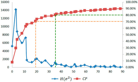
Figure 7.
The line graph of and for the example image.
3.3. Proposed Data Embedding Procedures
Along the same line as Peng et al.’s scheme, the proposed scheme performs maximum and minimum modification procedures to enhance the hiding performance. In the proposed scheme, the maximum value and the minimum value are used to embed the secret message. The shifting and embedding operation will change the original pixel at the most by 1 bit. Because the quantifying number is more than 2, the quantified value of the original pixel is the same as that of the stego pixel. The variance is invariant and can be recomputed by the decoder. Hence, the proposed scheme is reversible.
The embedding procedure is as shown.
- Divide the host image into several non-overlaping blocks sized . Let be the block and total number of blocks is .
- Sort each block in ascending order to get .
- Generate a location map to record whether the block has an overflow (or underflow) problem or not. For each block, if = 0 or = 255, then = 1 which means the block may have the problem. On the contrary, if = 0, the location map is then compressed by the data algorithm (such as arithmetic coding or JBIG2 and so on). The compressed results are then concatenated with the secret message to embed it into the host image.
- Compute the variance of each block by using Formulas (9)–(11).
- Calculate the predefined threshold using the adaptive threshold generation strategy which was introduced in Section 3.2.
- Detect whether the block is embeddable or not.
- If = 1, then the block is non-embeddable.
- If the variance and = 0, then the block is non-embeddable.
- If the variance and = 0, then the block is embeddable.
- Conceal the secret message into the embeddable block.
- Compute , where:
- Calculate the stego pixel by:
- Compute , where:
- Calculate the stego pixel by:
- Continue the steps until all secret messages are embedded.
The proposed scheme applies Wang et al.’s strategy to handle location mapping. Hence, the compressed location map is also concealed in the original image.
Figure 8 shows an embedding example by using the proposed scheme. For the first block X = {5, 4, 15, 19}, the proposed scheme first sorts the block according to its pixel values. The sorted block is . Before computing the variance of the block, the proposed scheme quantifies the block to get the quantified pixels. Suppose the quantifying number is , the block is quantified as , where and so on. Then, the variance of is computed by and . Assume that the threshold is . The variance is less than the threshold, . Hence, the block is embeddable. The proposed scheme calculates the distance between and to get , where = . Because the distance is higher than 1, the stego pixel of is set to be , where
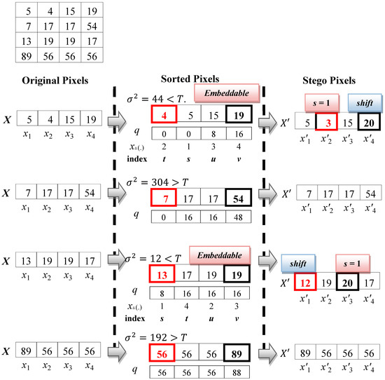
Figure 8.
Embedding example of the proposed scheme.
Next, the proposed scheme calculates the distance between and to get , where = . Because the distance is equal to 1, one secret bit can be concealed in the pixel. Assume that the secret bit is . The stego pixel is computed by = .
Consider another example, the second block is X = {7, 17, 17, 54}. Because the variance of the block is , the block is non-embeddable. The proposed scheme will skip the block and will not modify the pixel value.
Different from the previous work, the proposed scheme avoids shifting pixels located in complex areas where it is impossible to hide secret data. Hence, the image quality can be maintained in the proposed scheme.
3.4. Extraction and Recovering Procedures
When the receiver gets the stego image, they can use the extraction and recovering procedure to decode the secret bit and recover the original image. The procedures are shown below.
- Divide the stego image into several non-overlap blocks sized . Let be the block and total number of blocks is .
- Sort each block in ascending order to get .
- Extract the location map from the stego image by using Wang et al.’s scheme. For each block, if = 1 which means the block is non-embeddable.
- Compute the variance of each block by using Formulas (9)–(11).
- Detect whether the block is embeddable or not.
- If = 1, then the block is non-embeddable.
- If the variance and = 0, then the block is non-embeddable.
- If the variance and = 0, then the block is embeddable.
For the non-embeddable block, the proposed scheme will skip the block. The original block is the same as the stego block. - Extract the secret message from the embeddable block.
- Compute , where
- Obtain the secret message
- Calculate the original pixel by
- Compute , where
- Obtain the secret message
- Calculate the original pixel by
- Continue the steps until all the secret messages are extracted and the pixels are recovered.
Figure 9 shows an extraction example using the proposed scheme. In the first set = {5, 3, 15, 20}, the proposed scheme sorts the set according to its pixel values. The sorted set is . Before computing the variance of the set, the proposed scheme quantifies the set to get the quantified pixels. The quantifying number is ; hence, the set is quantified as , which is the same as the quantified number in the embedding procedure. Then, the variance of is . The threshold is , where , the set is embeddable. Then, the proposed scheme calculates the distance between and to get , where = . Because the distance is higher than 1, the original pixel of is , where
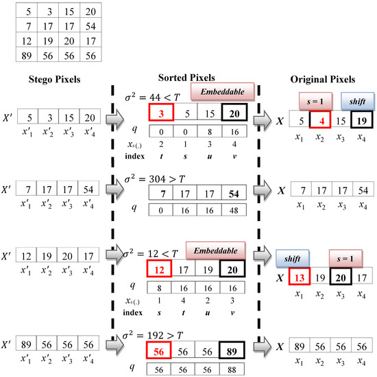
Figure 9.
Extraction and recovery example of the proposed scheme.
Next, the proposed scheme calculates the distance between and to get , where = . Because the distance is equal to 2, one secret bit can be concealed in the pixel. The secret bit is computed by = 2 − 1 = 1. The stego pixel is computed by = .
4. Experimental Results
The proposed scheme used six grayscale-images sized 512 × 512, namely as shown from left to right, top to bottom: Airplane, Lake, Lena, Mandrill, Pepper, and Tiffany so as to compare the performance with other methods. The images are shown in Figure 10.

Figure 10.
Six test images sized 512 × 512.
The comparisons utilize a peak signal to noise ratio (PSNR) to evaluate the image quality of the stego-images. The higher the PSNR value, the less perceptible the stego image will be. PSNR value is computed using:
where and is the width and height of an image.
The hiding payload is calculated using:
and the hiding rate is calculated by:
where is the total number of secret bits embedded in the cover image, and means the total number of bits embedded in the current stage.
In Section 4.1, a systematic way is designed to determine the adaptive threshold value of T. Each image is evaluated based on its own threshold. In Section 4.2, a comparison is made between the hiding capacity and image quality for the proposed method as it relates to Peng et al. and Wang et al.’s schemes.
4.1. Adaptive Threshold Detection
In the embedding procedure, a proper threshold T, which is used to determine whether the block is embeddable or not, is very important. To find the appropriate threshold, the proposed scheme examines the variances of each image and analyzes the tendency of the variance curve. The statistical variance curves of the test images are shown in Figure 11.
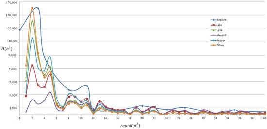
Figure 11.
The variance curves for the test images.
Table 2 shows the threshold values of the test images under different hiding rates. For example, for the hiding rate set of 70%, the threshold of Lena is equal to T = 20 that cumulative percentage (CP) is 71.33%. On the contrary, for the hiding rate set of 80%, the threshold is equal to T = 36 which is CP = 80.46%.

Table 2.
The threshold value T of each image in the different hiding rate.
4.2. Quantified Number Evaluation
The value of is used to quantify the pixel such that the quantified original pixel is equal to the quantified stgeo pixel. Figure 12 shows the experimental results of the test image under different hiding rates with = 4 and = 8. For example, the symbol VAR (70, ) means the hiding rate is set of 70% and = 4.
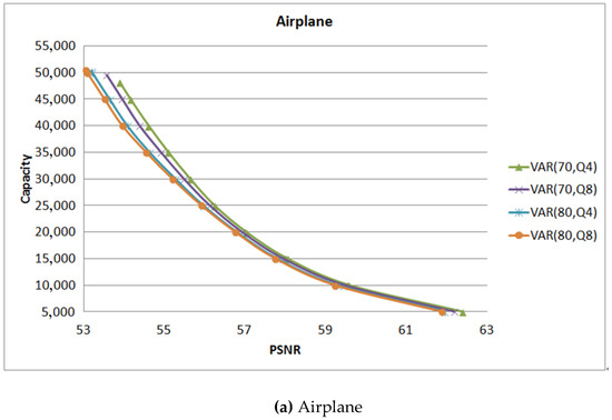
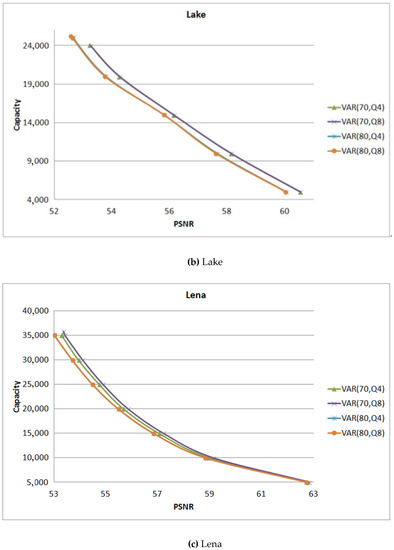
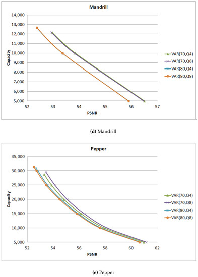
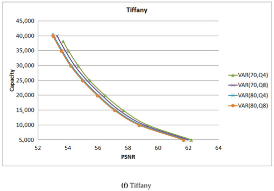
Figure 12.
The comparison between different values.
For the smooth images Airplane shown in Figure 12a and Tiffany shown in Figure 12f, when the hiding rate is set of 70%, = 4 can get a better image quality and hiding capacity. But for the images Lena shown in Figure 12c and Pepper shown in Figure 12e, the performance of = 8 is a little higher than that of = 4. For the complex images Mandrill shown in Figure 12d and Lake shown in Figure 12b, there is no difference between the values of . Therefore, in the smooth image, the value of is suggested to be set as 4. On the contrary, the proposed scheme suggests should be set to 8.
4.3. Comparison Results
The proposed scheme improves upon Peng et al.’s scheme with variance detection, hence the proposed scheme is called Peng_VAR. The experiment that compares the proposed scheme to Peng et al. (called Peng) and Wang et al.’s (called Wang) scheme is shown in Table 3. For the image Airplane, the capacities of the proposed scheme Peng_VAR with hiding rates of 70% and 80% are 48,132, and 50,223 bits. Peng’s and Wang’s schemes are 52,546 and 52,007, respectively. Although the hiding capacity of the proposed scheme is less than Peng and Wang’s schemes, the PSNR values of the proposed scheme are higher than that of the others. The PSNR value of the proposed scheme with a hiding rate of 70% is 53.90 which is more than that of Peng’s scheme 1.79 dB and that of Wang’s scheme 1.69 dB.

Table 3.
The comparison results between the proposed scheme and the other schemes.
The column “Increased” in Table 3 is the difference of PSNR between Peng_VAR 70% and other schemes. For example, the difference of PSNR between Peng_VAR 70% and Peng is 1.79 = 53.90 − 52.11. The average PSNR value of the proposed scheme with a hiding rate of 70% is higher than that of Peng’s scheme 1.63 dB and that of Wang’s scheme 1.14 dB. With a hiding rate of 80%, the proposed scheme surpasses Peng’s scheme 1.01 dB and Wang’s scheme 0.52 dB.
Figure 13 shows the experimental results of the proposed scheme and the other schemes. Peng_VAR (70%) and Peng_VAR (80%) are the proposed schemes with hiding capacities of 70% and 80%, respectively. Both of the figures show that Peng_VAR (70%) can get highest PSNR value, particularly for complex images such as Mandrill and Lake. The figure also shows that under the same hiding capacity, the PSNR value of the proposed scheme is better than that of the other schemes. For example, if the hiding capacity was set to be 30,000, the PSNR value of the proposed scheme is 53.95 dB and that of Peng’s scheme and Wang’s scheme are 53.01 and 53.26 dB, respectively.
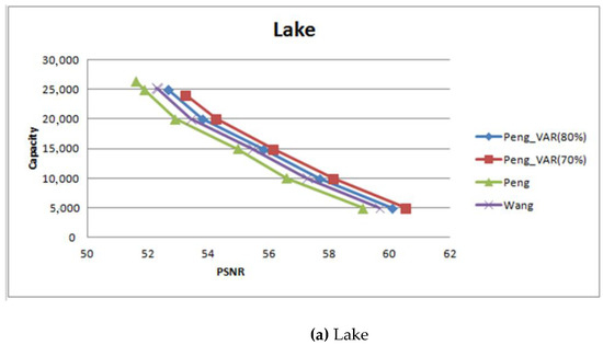
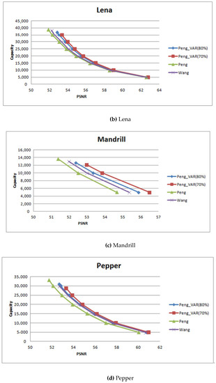
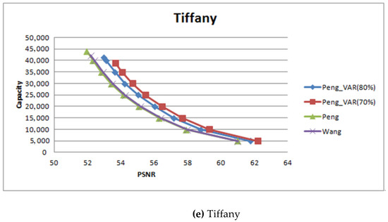
Figure 13.
The experimental results of different hiding capacity.
To prove that the proposed scheme was not designed for some special image, the images from the Uncompressed Color Image Database (UCID) (http://homepages.lboro.ac.uk/~cogs/datasets/ucid/ucid.html) were included to test the performance of the proposed scheme. There are 1338 color images sized 512 × 384 (or 384 × 512) in UCID database. Some of them are shown in Figure 14. Before performing the experiment, these images were transformed to gray-scale. The proposed scheme converts RGB values to gray-scale values by forming a weighted sum of the R, G, and B components. The equation is shown below:

Figure 14.
Some test images from Uncompressed Color Image Database (UCID).
Figure 15 and Figure 16. depict the PSNR and hiding capacity comparisons among the proposed scheme and the other schemes. In Figure 16, so as to show the tendency, the proposed scheme used the PSNR value of Peng_VAR (80%) to sort the images in increasing order. In general, the PSNR values of Peng_VAR (70%) are higher than that of the others. There are 135 images hiding by using Wang’s scheme where the PSNR value is higher than the proposed scheme. Some of them are shown in Table 4. Most with high PSNR value have a low hiding capacity. Furthermore, the total number of pixels which has an overflow or underflow problem is the highest among the comparison schemes. For example, for the image numbered 1063, the total number of overflow pixels is 453. Furthermore, these 135 images are very complex.
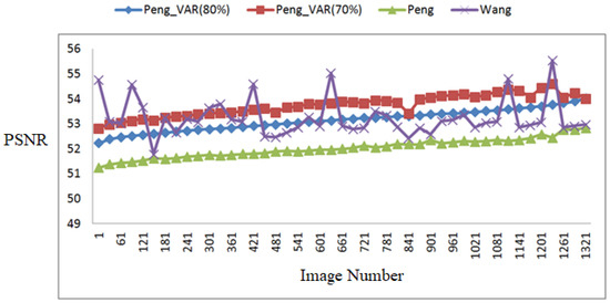
Figure 15.
Peak signal to noise ratio (PSNR) comparison using UCID images.
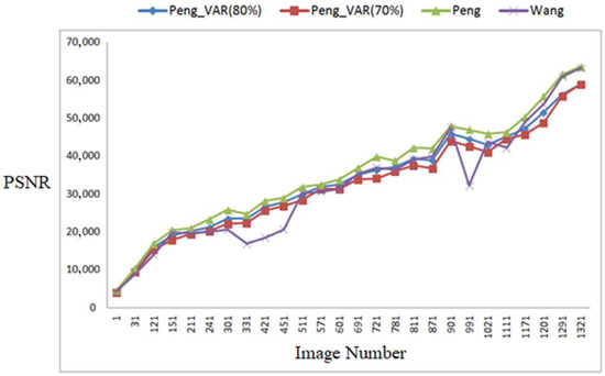
Figure 16.
Hiding capacity comparison using UCID images.

Table 4.
Some images of the 135 special case images.
Table 5 shows some comparison results by using UCID database. The PSNR value of the proposed scheme with a hiding rate of 70% averages higher than that of Peng’s scheme 1.7 dB and that of Wang’s scheme 0.8 dB. The hiding capacity of the proposed scheme on average is only less than that of Peng’s scheme by 3301 bits and that of Wang’s scheme by 307 bits. For the hiding rate set of 80%, the PSNR value of the proposed scheme on average is higher than that of Peng’s scheme 1.1 dB and that of Wang’s scheme 0.22 dB. The hiding capacity of the proposed scheme on average is less than that of Peng’s scheme by 1985 bits, but the hiding capacity of the proposed scheme is higher than that of Wang’s scheme by 1331 bits.

Table 5.
Some comparison results by using UCID database.
5. Conclusions
In order to solve Peng’s threshold problem, this study proposed an adaptive threshold generation strategy. After computing the variances of each block, the proposed scheme can decide a suitable threshold according to the hiding rate, and the sender can set the hiding rate. Because of the threshold, some blocks may have overflow or underflow problems, which can be avoided. In addition, the proposed scheme does not modify the non-embeddable block, so the image quality can be maintained. This study adopts a quantification mechanism to ascertain the receiver can get the same quantified pixels as the sender. The quantifying number is suggested as set at 8 for complex images.
According to the experimental results shown in Table 3, the PSNR value of the proposed scheme with a hiding rate of 70% is higher than that of Peng’s scheme, 1.63 dB, and that of Wang’s scheme 1.14 dB. With a hiding rate of 80%, the proposed scheme surpasses Peng’s scheme 1.01 dB and Wang’s scheme 0.52 dB. Table 4 shows that the PSNR value of the proposed scheme with a hiding rate of 70% averages higher than that of Peng’s scheme 1.7 dB and that of Wang’s scheme 0.8 dB. The hiding capacity of the proposed scheme on average is only less than that of Peng’s scheme by 3301 bits and that of Wang’s scheme by 307 bits. For the hiding rate set of 80%, the PSNR value of the proposed scheme on average is higher than that of Peng’s scheme 1.1 dB and that of Wang’s scheme 0.22 dB. The hiding capacity of the proposed scheme on average is less than that of Peng’s scheme by 1985 bits, but the hiding capacity of the proposed scheme is higher than that of Wang’s scheme by 1331 bits.
Based on the experimental results, we can see that the proposed scheme indeed improved the image quality of Peng’s scheme. Furthermore, the hiding capacity of the proposed scheme with a hiding rate of 80% is higher than that of Wang’s scheme.
Author Contributions
T.-C.L. designed the algorithm, conducted all experiments, analyzed the results, and wrote the manuscript. C.-Y.T. conceived the algorithm and wrote the manuscript. S.-W.H. conducted the literature review and wrote the manuscript. T.N.V. wrote the manuscript.
Funding
Taiwan’s Ministry of Science and Technology grant number MOST 107-2637-E-324-004-.
Acknowledgments
This study was financially supported by a research grant from Taiwan’s Ministry of Science and Technology (MOST 107-2637-E-324-004-).
Conflicts of Interest
The authors declare no conflict of interest.
References
- Ou, B.; Li, X.; Zhao, Y.; Ni, R. Reversible Data Hiding Based on PDE Predictor. J. Syst. Softw. 2013, 86, 2700–2709. [Google Scholar] [CrossRef]
- Ni, Z.; Shi, Y.Q.; Ansari, N.; Su, W. Reversible Data Hiding. IEEE Trans. Circuits Syst. Video Technol. 2006, 16, 354–362. [Google Scholar]
- Meikap, S.; Jana, B. Directional PVO for Reversible Data Hiding Scheme with Image Interpolation. Multimedia Tools Appl. 2018, 77, 31281–31311. [Google Scholar] [CrossRef]
- Tian, J. Reversible Data Embedding Using a Difference Expansion. IEEE Trans. Circuits Syst. Video Technol. 2003, 13, 890–896. [Google Scholar] [CrossRef]
- Lu, T.C.; Tseng, C.Y.; Wu, J.H. Asymmetric-Histogram Based Reversible Information Hiding Scheme Using Edge Sensitivity Detection. J. Syst. Softw. 2016, 116, 2–21. [Google Scholar] [CrossRef]
- Thodi, D.M.; Rodriguez, J.J. Expansion Embedding Techniques for Reversible Watermarking. IEEE Trans. Image Process. 2007, 16, 721–730. [Google Scholar] [CrossRef]
- Luo, T.; Jiang, G.; Yu, M.; Gao, W. Novel Prediction Error Based Reversible Data Hiding Method Using Histogram Shifting. Int. J. Comput. Theory Eng. 2015, 7, 332–336. [Google Scholar] [CrossRef]
- Hong, W.; Chen, T.S.; Shiu, C.W. Reversible Data Hiding for High Quality Images Using Modification of Prediction Error. J. Syst. Softw. 2009, 82, 1833–1842. [Google Scholar] [CrossRef]
- Fallahpour, M. Reversible Image Data Hiding Based on Gradient Adjusted Prediction. IEICE Electron. Express 2008, 5, 870–876. [Google Scholar] [CrossRef]
- Coltuc, D. Improved Embedding for Prediction-Based Reversible Watermarking. IEEE Trans. Inf. Forensics Secur. 2011, 6, 873–882. [Google Scholar] [CrossRef]
- Li, X.; Zhang, W.; Gui, X.; Yang, B. A Novel Reversible Data Hiding Scheme Based on Two-Dimensional Difference-Histogram Modification. IEEE Trans. Inf. Forensics Secur. 2013, 8, 1091–1100. [Google Scholar]
- Wu, X.; Memon, N. Context-Based, Adaptive, Lossless Image Coding. IEEE Trans. Commun. 1997, 45, 437–444. [Google Scholar] [CrossRef]
- Lu, T.C.; Tseng, C.Y.; Deng, K.M. Reversible Data Hiding Using Local Edge Sensing Prediction Methods and Adaptive Thresholds. Signal Process. 2014, 104, 152–166. [Google Scholar] [CrossRef]
- Feng, G.; Fan, L. Reversible Data Hiding of High Payload Using Local Edge Sensing Prediction. J. Syst. Softw. 2012, 85, 392–399. [Google Scholar] [CrossRef]
- Lukac, R.; Martin, K.; Plataniotis, K.N. Digital Camera Zooming Based on Unified CFA Image Processing Steps. IEEE Trans. Consum. Electron. 2004, 50, 15–24. [Google Scholar] [CrossRef]
- Bo, O.; Li, X.L.; Wang, J.W. Improved PVO-based Reversible Data Hiding: A new Implementation based on Multiple Histograms Modification. J. Vis. Commun. Image Represent. 2016, 38, 328–339. [Google Scholar]
- He, W.G.; Cai, J.; Zhou, K.; Xiong, G.Q. Efficient PVO-based Reversible Data Hiding Using Multistage Blocking and Prediction Accuracy Matrix. J. Vis. Commun. Image Represent. 2017, 46, 58–69. [Google Scholar] [CrossRef]
- Li, X.; Li, J.; Li, B.; Yang, B. High-Fidelity Reversible Data Hiding Scheme Based on Pixel-Value-Ordering and Prediction-Error Expansion. Signal Process. 2013, 93, 198–205. [Google Scholar] [CrossRef]
- Peng, F.; Li, X.; Yang, B. Improved PVO-Based Reversible Data Hiding. Digit. Signal Process. 2014, 25, 255–265. [Google Scholar] [CrossRef]
- Wang, X.; Ding, J.; Pei, Q. A Novel Reversible Image Data Hiding Scheme Based on Pixel Value Ordering and Dynamic Pixel Block Partition. Inf. Sci. 2015, 310, 16–35. [Google Scholar] [CrossRef]
- Weinberger, M.J.; Seroussi, G.; Sapiro, G. The LOCO-I Lossless Image Compression Algorithm: Principles and Standardization into JPEG-LS. IEEE Trans. Image Process. 2000, 9, 1309–1324. [Google Scholar] [CrossRef] [PubMed]
© 2018 by the authors. Licensee MDPI, Basel, Switzerland. This article is an open access article distributed under the terms and conditions of the Creative Commons Attribution (CC BY) license (http://creativecommons.org/licenses/by/4.0/).


