Emotion Classification Using a Tensorflow Generative Adversarial Network Implementation

Abstract

The detection of human emotions has applicability in various domains such as assisted living, health monitoring, domestic appliance control, crowd behavior tracking real time, and emotional security. The paper proposes a new system for emotion classification based on a generative adversarial network (GAN) classifier. The generative adversarial networks have been widely used for generating realistic images, but the classification capabilities have been vaguely exploited. One of the main advantages is that by using the generator, we can extend our testing dataset and add more variety to each of the seven emotion classes we try to identify. Thus, the novelty of our study consists in increasing the number of classes from N to 2N (in the learning phase) by considering real and fake emotions. Facial key points are obtained from real and generated facial images, and vectors connecting them with the facial center of gravity are used by the discriminator to classify the image as one of the 14 classes of interest (real and fake for seven emotions). As another contribution, real images from different emotional classes are used in the generation process unlike the classical GAN approach which generates images from simple noise arrays. By using the proposed method, our system can classify emotions in facial images regardless of gender, race, ethnicity, age and face rotation. An accuracy of 75.2% was obtained on 7000 real images (14,000, also considering the generated images) from multiple combined facial datasets.

1. Introduction

Face detection and recognition has been an on-going research area for the last 50 years, with concluding results being obtained starting with the late 90s [1]. The fast development of facial recognition technology allowed it to be used in a variety of areas like assisted living, health monitoring, access control, authentication, ID/passport control and fraud prevention, security/law enforcement (to identify lawbreakers or terrorists), surveillance systems, attendance tracking and counting and many others. According to a report published by MarketsandMarkets in 2017 [2], the global facial recognition market was estimated at 3.37 billion USD in 2016 and it is expected to grow up to 7.76 billion USD by 2022, with an annual growth rate of 13.9%.

Various methods have been used for facial detection and localization, and reviews of those methods are presented in References [3,4,5]. Different methods vary from template matching and knowledge-based methods to support vector machines, hidden Markov models and principal component analysis. The reviews concluded that the obtained accuracies for detection kept improving with each new method, but the selected samples for research were limited and had little variety, with good accuracies being obtained only on specific datasets. Neural networks-based face recognition improved the results of all previous methods and also brought an increase in efficiency and execution time. A variety of reviews [6,7,8,9,10,11,12,13,14] compare the advantages, disadvantages and results of multiple different neural network methods. The reviews mark the importance of CNNs (convolutional neural networks) and deep learning in the area of facial recognition, deep learning specifically being considered a huge step in the evolution of facial recognition algorithms. Most of the presented researches have accuracies over 90% on public available datasets, but different challenges are still acknowledged regarding real-world facial recognition, training the algorithms to replicate human behavior and large scale adoption in the industry. Different approaches are presented in References [15,16], where fuzzy algorithms perform a rotation invariant face recognition based on symmetrical facial characteristics. The main advantage is that the algorithms can be used on smart TVs (Television sets) with low processing power to recognize the viewer and offer proper content and services accordingly. The algorithm presented in Reference [16] is an enhanced version of the one in Reference [15], with an increase in accuracy. The presence of cosmetics and contact lenses adds challenges to face recognition for biometric purposes. Color, shape and texture features of the face and iris are extracted in Reference [17] to be used in a SVM (support vector machine) classifier for face recognition regardless of the makeup. The research shows improvement over several other face recognition methodologies. Another method was also developed in Reference [18], for makeup-invariant face verification, making use of the generative adversarial network (GAN) architecture first introduced in Reference [19]. The algorithm synthesizes non-makeup images from makeup images so that they can be used for face verification. The algorithm outperforms competing algorithms in terms of accuracy, speed, and size of the training dataset.

The introduction of GAN in Reference [19] opened new possibilities for image generation algorithms [20], including facial images. In this case, the generator (G) component is used to synthesize new images, while the discriminator (D) should detect the fake generated images. The G and D learn to improve by playing a minimax game which each of the components tries to win. There are two possible outcomes when using and training GANs. If more focus is put on the generator, then an image synthesis system is obtained. Otherwise, if the generator is used only to create images for the discriminator to assess, the D component can be used as a classifier. In Reference [21], a conditional GAN is used to generate facial images from simple noise and conditional data. This extension of the basic GAN is the first GAN model used strictly for facial generation. GANs can also be used to synthesize an aged version of the input image, as seen in Reference [22]. Although the results can’t be validated, the obtained images are highly realistic. Other use cases for GAN include generating front-faced images from rotated images [23], altering images (closing/opening eyes/mouth) while preserving identity of the person illustrated in the images [24], and also removing extra lighting from facial images to ensure proper conditions for face identification [25]. The last three techniques prove the utility of GANs in image processing. The generator is trained in [26] to reconstruct 2.5-D images from 2-D images, and the output is used in two other CNNs (convolutional neural networks) for feature extraction and face recognition. Different training techniques for GANs are presented in References [27,28,29,30,31], covering unsupervised, semi-supervised, and supervised learning and also providing different outputs for classifiers:

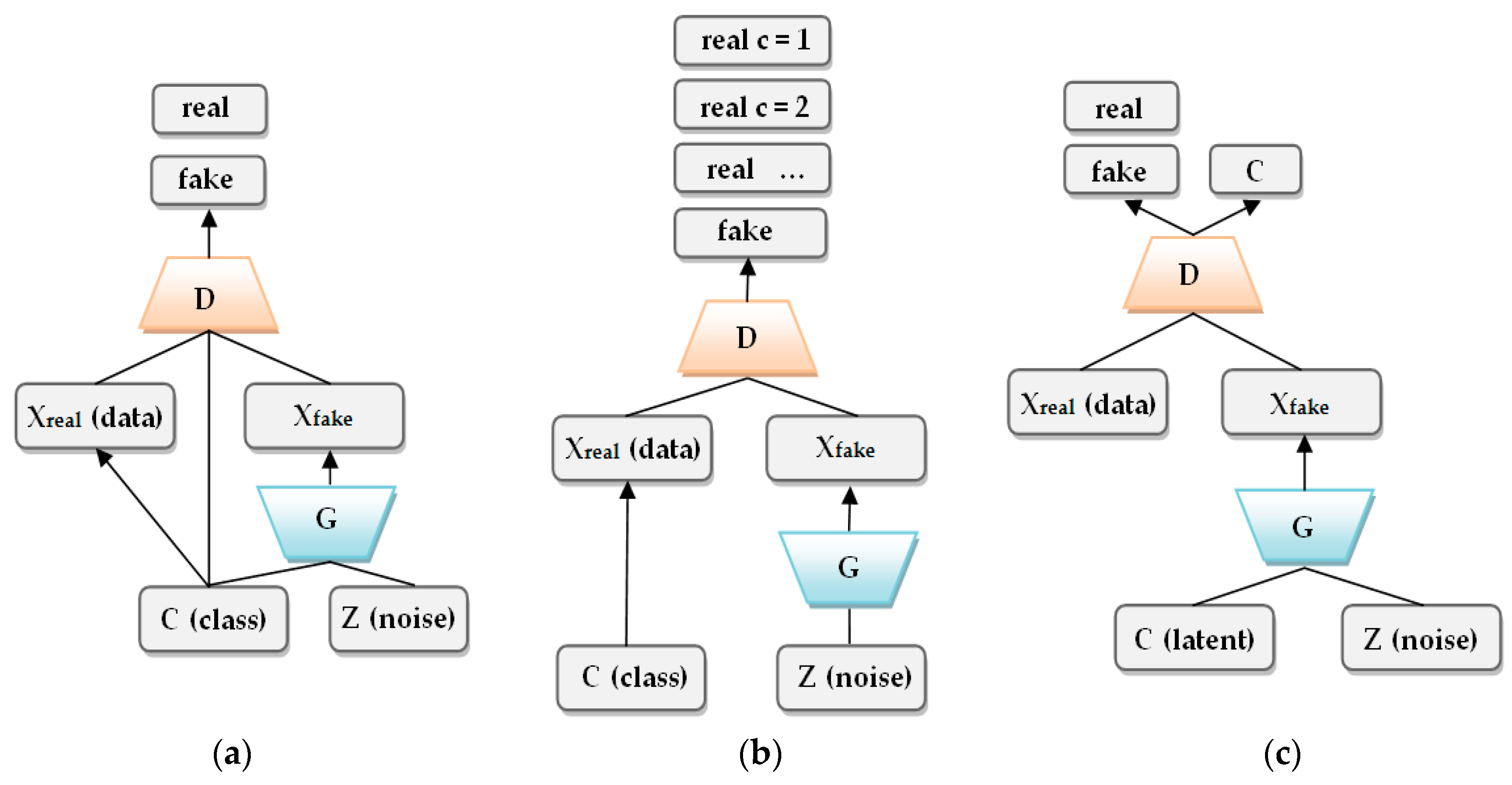
• Class conditional models: condition the G to produce an image in a specific class and use the D to assert whether the image is fake or real (two output classes)
• N-output classes [27]: Use the D to classify the input image in various classes; ideally, the generated images should have a low level of confidence for the output class. The semi-supervised learning approach almost leads to the best performance in classifying images containing numbers or different objects. Unfortunately, the unsupervised approach has proven a weak accuracy in multiple-class classification.
• N+1-output classes [29,30,31]: Use the N-classes approach but also have a distinct class for generated images. The semi-supervised trained classifier in Reference [29] is a more data-efficient version of the regular GAN, delivering higher quality and requiring less training time. The research has been conducted on the MNIST database (Modified National Institute of Standards and Technology database). The same conclusion was also reached in References [30] and [31] by the creators of the original GAN, but with an expanded dataset containing images of different objects, animals and plants.

2. Related Work

Emotion recognition is a new sub-area of facial recognition with high potential. Applications that perform emotion recognition can be used in various areas, like marketing (products/services evaluation and feedback based on customer emotions), psychology (identifying criminal profiles or terrorists before committing an attack), security (replace the panic button with fear detection during a robbery or an assault), and even medicine [32,33,34,35] (effects of positive and negative emotions on the patients’ health using current technology). Although performed before the development of modern emotion recognition techniques, the presented medical studies show the importance of emotion monitoring as a step in detecting depression and other diseases. Most progress in using GANs in the domain of emotion is represented by the possibility of altering an emotion in an image based on labeled information about the target emotion [36,37,38,39,40,41]. The obtained images are highly realistic and hard to distinguish as fake by human observers. The method in Reference [36] and its improved version [41] generate a sketch image of the emotion from an image, its emotion label and random noise. The sketch is assessed by the discriminator for correctness and then used as input in another GAN which generates an image of another person with the same facial emotion. The generated facial expressions are compared with real valid facial expressions, having the distances between the two classes reported as small.

A starting point in emotion recognition is represented by the identification of facial regions of interest, which can be done by localizing a series of facial key points. These features describe the position, shape, and size of the corresponding regions of interest. In Reference [42], a lip contour detection and tracking system is presented. The system uses a multi-state mouth model that represents different mouth states, a series of lip templates, and shape, color and motion information. The facial points associated with the lip are tracked in the image sequence and the lip contour is obtained from the template parameters, with the color and shape information being used to distinguish different lip states. A neural network for the detection of 15 facial key points is described in Reference [43]. The proposed deep convolutional neural network uses a learning model for each facial key point with the result outperforming other similar approaches. A total of 194 facial landmarks are estimated for each facial image in Reference [44] by using an ensemble of regression trees. The obtained predictions are of high quality, with the algorithm also performing in real-time. The paper also includes optimizations for improving feature selection, a comparison of different regularization strategies, and a study on the evolution of predictions based on the quantity of training data. Facial micro-expressions are analyzed in Reference [45] using 31 facial points out of the 121 obtained using the Kinect face tracking API (Application Programming Interface). The micro expressions are analyzed based on different visual and auditory stimuli, as well as the gender of the subjects. The authors also studied the possibility to distinguish emotions based on the results.

Two different neural networks for emotion recognition are trained and compared in Reference [46]. The first approach is to use representational autoencoder units. Four autoencoders were developed and tested on the JAFFE (Japanese Female Facial Expression) [47] and LFW (Labeled Faces in the Wild) [48] facial images datasets with accuracies of 60% and 49% respectively. The other selected implementation is an eight-layer convolutional neural network, created and trained from scratch. The network includes convolutional, max pooling, and fully connected layers. Using the same datasets [47,48], the accuracy increased to 86% and 67%, respectively, after 20 epochs and 420 iterations. In Reference [49] a CNN classifier is developed and trained on the FER2013 dataset [50]. Due to differences in the number of images for each emotion class, two cycle-GANs are trained to generate disgust and sadness images starting from neutral face images. Therefore, the training dataset is expanded for an equal distribution of images. Using the generated images, the overall accuracy of the CNN classifier improved. Further testing with good results is performed on other datasets [47,48,50]. A fear estimation system is developed in Reference [51], using two images captured by a dual camera system: a near infrared (NIR) camera (Logitech, CA, USA) and a thermal camera (FLIR, OR, USA). Seven different features are extracted from the two images (two from thermal images and five from NIR images) and the last feature is represented by the direct input of the study subjects via a real time questionnaire. The algorithm proposed in [44] is used to extract 68 facial feature points for the NIR images. The extracted feature points are further used to compute the five features based on facial point movement between successive images of the subject who switches from neutral to scared (fear). The top four discriminatory features are selected and their values are normalized (0–1) and used as input in a fuzzy inference system, which evaluates the value of the fear emotion from low to high.

The authors in Reference [52] develop and train two convolutional neural networks with different scale invariant features. The feature descriptors are represented by image gradients computed using key points neighboring pixels of the given image, on 4 × 4 patches (16 patches for each image). K-means clustering is used to group the feature descriptors in clusters for each emotion. The proposed models are trained on FER [50] and CK+ [53] datasets and tested on an additional dataset, SFEW [54]. The reported results have a good accuracy on the training dataset, but a decreased one for the third dataset. In Reference [55], two methods for emotion recognition are proposed: SVM and CNN. The different SVM models (one-vs-one, principal component analysis, one-vs-all, histogram of oriented gradients) presented issues during training and obtained lower accuracies on all the tested datasets. Several other CNN implementations with additional preprocessing techniques were tested. The best obtained accuracy on a small subset of FER [50] was 66.67%. The algorithm is further used for real-time image classification in video feeds. Five existing CNN approaches for deep learning are proposed, adjusted, and compared in [56], with the scope of emotion recognition. The input images are preprocessed using the Viola-Jones algorithm. Then, existing models are adjusted (adding new layers), trained and tested for accuracy. A CNN with two similar sequences of two convolutional layers and a sub-sampling layer, followed by a dense layer with 3072 filters and an output layer, obtained the best accuracy (63%).

The current paper proposes a new system for emotion classification based on a GAN classifier. The facial emotions are classified within seven emotions–anger, disgust, fear, happiness, neutral, sadness, and surprise. To this end, 14 classes are used to train the GAN–a real class and a fake one of each emotion. The novelty of the proposed method is brought by using the new 2N-classes approach for training the GAN classifier which normally operates with N-classes. As a consequence, the detection accuracy increased. Another contribution is the expansion of the test images dataset by generating images using the GAN. Real images of a different class are used in the generation process, which is different from the standard GAN approach to generate images from a simple noise array. By only using the rotation-invariant facial points as input for the classifier, we also reduce the amount of data that is analyzed. The facial-points vectors are processed to be rotation insensitive, so that tilted facial images can also be classified, as opposed to similar presented algorithms, which can classify only front faced facial images. The remainder of the paper is organized as follows: In Section 3, the methodology and architecture of the proposed system are described. In Section 4, the experimental results are presented, along with a performance analysis. The paper concludes with the discussions in Section 5 and Section 6.

3. Materials and Methods

3.1. Training and Evaluation Phase

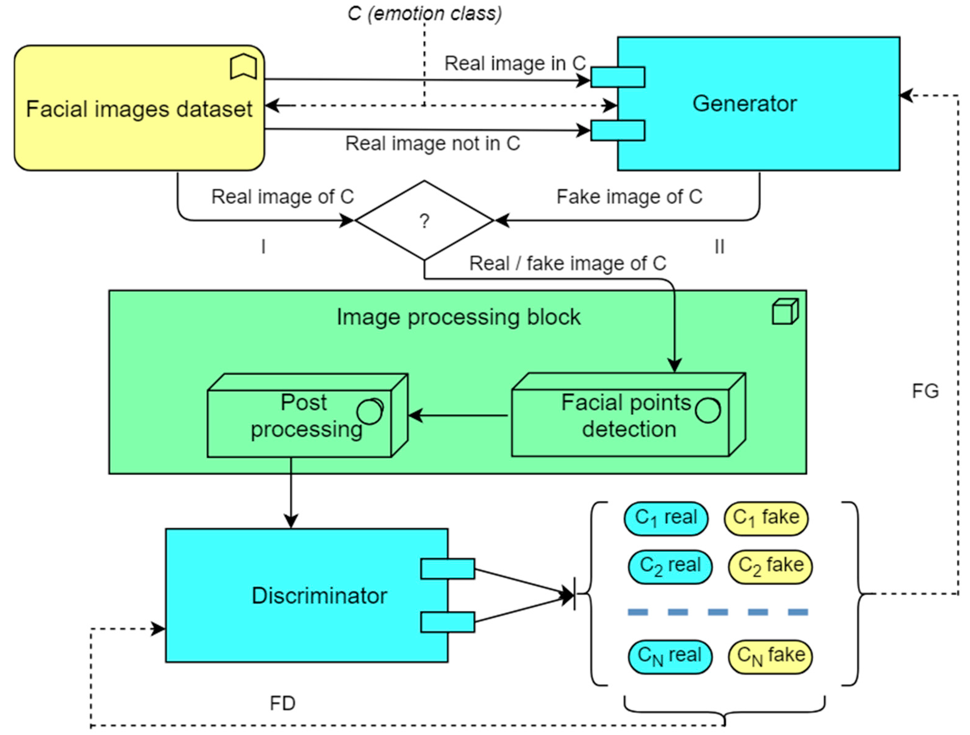
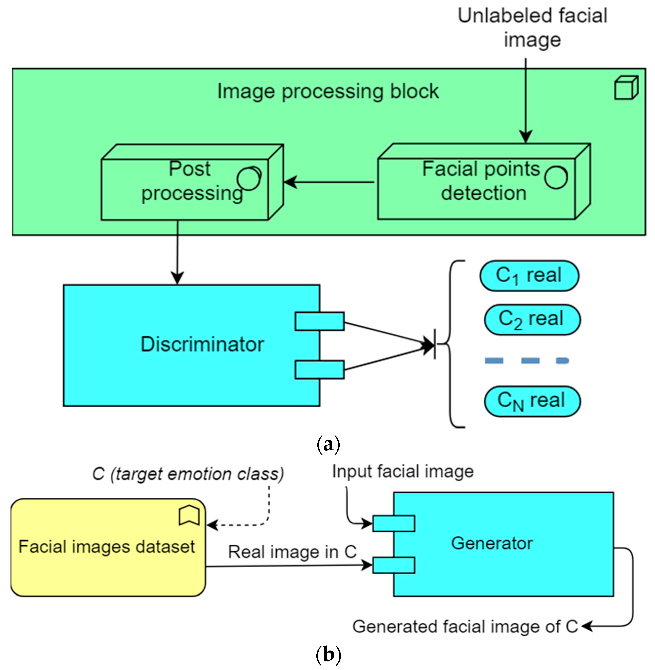
3.1.1. System Architecture

Robert Plutchik [57] developed a wheel of emotions, stating that there are eight primary emotions: happiness (joy), sadness, anger, fear, trust, disgust, surprise, and anticipation, which can have a variety of intensities. The primary emotions are located on the first ring. Moreover, complex emotions can be obtained from a mix of primary emotions (with a distance of 1, 2 or 3 on the wheel), thus obtaining the full spectrum of human emotions.

We propose a system for the classification of six primary emotions (happiness, sadness, anger, fear, disgust, and surprise) in facial images, adding another class of neutral emotion (lack of a dominant emotion). Five emotions are negative, with happiness being the only positive. The system is based on a modified conditional GAN. The first proposed implementation of a GAN [19] had a simple structure. The discriminator D would receive either a real image or a fake (generated) image and would have to assess it as real or fake. The generator G was responsible with generating a fake image similar to the real one, starting from simple noise and a latent space vector. Based on the correctness of the decision, the discriminator and generator would adjust their weights. The discriminator and generator play a minimax two-player game with the value function in Equation (1):

$$\underset{\mathrm{G}}{\min }\underset{\mathrm{D}}{\max }V\left(\mathrm{D},\mathrm{G}\right)= E_{x~p_{data}\left(x\right)}\left[\log \mathrm{D}\left(x\right)\right]+E_{z~p_z\left(z\right)}\left[\log \left(1-\mathrm{D}\left(\mathrm{G}\left(z\right)\right)\right)\right]$$

(1)

The first term of the equation is represented by the entropy (E) passed by the distribution of the real data (p_data(x)) through the discriminator (D(x)) and it can have a maximum value of 1. The second term is represented by the entropy passed by the distribution of the random noise input (p(z)) through the generator (G(z)) that produces a fake data sample which is further passed to the discriminator for assessment. The second term can have a maximum value of 0. The discriminator tries to maximize the value function V(D,G) (meaning that the fake data is always labeled as fake), while the generator tries to minimize the value function (in this case the difference between the real and the fake data is minimum)

Starting from the original network structure, several varieties of GAN architectures were proposed, as seen in Figure 1.

Our proposed architecture combines elements from the previous described implementations. The novelty is brought by using a real image not part of the desired class to generate the fake images, instead of using a noise vector, adding an image processing block for facial points extraction and constructing rotation invariant facial vectors, and splitting the real/fake assessment and class identification into a single 2N type classification (a real and a fake class for each emotion). The proposed architecture can be seen in Figure 2.

Each training cycle of the network is split into three phases. During the first phase (flow I—the left side of Figure 2), the generator is switched off and the discriminator receives only real class-labelled images. The discriminator adjusts its weights based on the feedback loop FD. For the first phase of the first training cycle, the discriminator will only use the N real classes as possible outputs for an image. For any other phase or cycle, all the 2N classes are used. During the second phase (flow II– the right side of Figure 2), the discriminator remains unmodified and the generator is trained to deliver fake images of given classes which the discriminator has to classify. The generator uses the feedback loop FG to adjust weights. In the third phase (also flow II), the roles switch and the generator is kept unmodified, while the discriminator is trained with both real and fake images. The feedback loop FD is used for weights adjusting. The three main components (image processing block, discriminator and generator) are described in Section 3.1.2, Section 3.1.3, and Section 3.1.4, respectively.

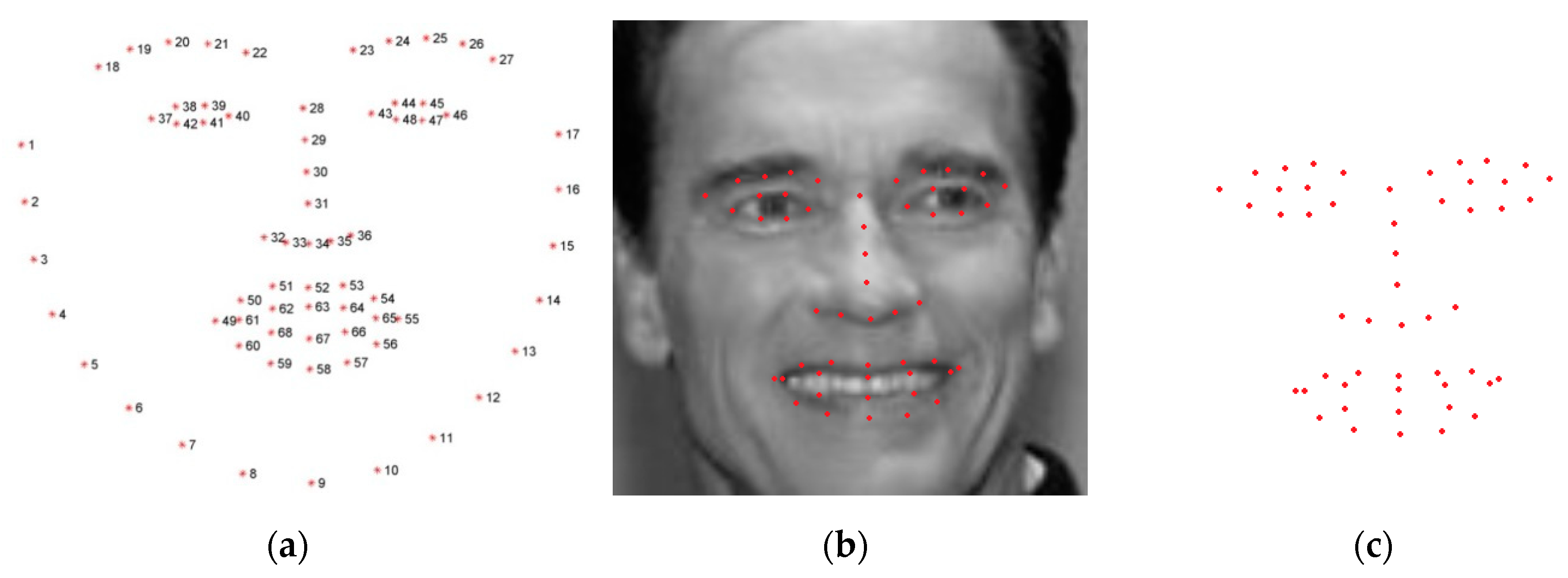
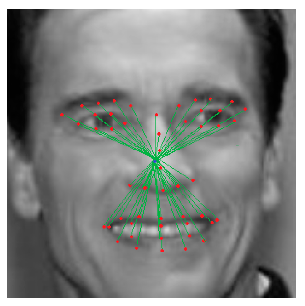
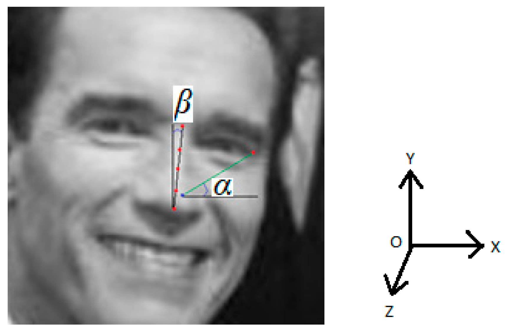
3.1.2. Image Processing Block

The image processing block acts as an intermediate between the input images (either real or generated) and the discriminator. We designed this block so that the discriminator can receive more meaningful information based on which it can classify the images. This block performs two main operations, namely the detection of facial-key points (detailed in Section A) and finding the correlation between these points (Section B). The image processing block is used to minimize the variations brought by gender, age, race, and head posture, while using a large range of test images. Similar works try to limit these variations by limiting the image dataset on which the algorithms are validated.

A. Facial Points Detection

Facial landmarks are regions of interest that can uniquely identify different components of the face, such as eyes, eyebrows, lips and nose. These landmarks can be described by a series of facial key points. In order to extract the facial feature points, we used the real-time face estimation open source code from dlib C++ library [59]. The code implements the method described in Reference [44]. The dlib library contains a pre-trained detector that estimates the coordinates of 68 points that are mapped on facial regions of interest. The implemented detector uses an ensemble of regression trees for facial feature tracking. The 68 labeled points output of the detector can be seen in Figure 3a, while Figure 3b,c show the result of applying the detection algorithm on a test image. Because most of the test images only contain a cropped image of the face, we will not use the full set of 68 points, but a smaller one of 51 (removing the 17 points associated with the jaw line).

The facial regions of interest can be described as follows (using the points from Figure 3a):

• Right eyebrow—points 18, 19, 20, 21 and 22;
• Left eyebrow—points 23, 24, 25, 26 and 27;
• Right eye—points 37, 38, 39, 40, 41 and 42;
• Left eye—points 43, 44, 45,46, 47 and 48;
• Nose—points 28, 29, 30, 31, 32, 33, 34, 35 and 36;
• Mouth:

  ○

  Upper outer lip—points 49, 50, 51, 52, 53, 54, and 55;

  ○

  Upper inner lip—points 61, 62, 63, 64, and 65;

  ○

  Lower inner lip—points 61, 65, 66, 67, and 68;

  ○

  Lower outer lip—points 49, 55, 56, 57, 58, 59, and 60.

B. Post Processing

In this module, we computed the relative position of the facial points relative to each other. In order to achieve this, we first computed the position of the facial center of gravity as the average position of all the other extracted points from Section A, using the Equation (2), where x_i represents the distance on the OX axis and y_i represents the distance on OY axis, from the center of origin O located in the lower left corner of the image.

$$x_{mean}=\frac{{{\displaystyle \sum }}_{i=18}^{68}{x}_i}{51} y_{mean}=\frac{{{\displaystyle \sum }}_{i=18}^{68}{y}_i}{51}$$

(2)

After determining the center of gravity, we computed the vectors that join the center of gravity and the other facial key points. Each of the vectors has a direction (angle relative to the horizontal axis) and a magnitude (distance from the center of gravity). In Figure 4, the center of gravity (blue dot), the facial key points (red dots) and the vectors connecting them (green lines) can be observed. Also, symmetry between vectors corresponding to the same points on the left and right sides of the face can be observed.

The center of gravity was selected as reference over any of the points because of the variance the different points bring depending on the face morphology. This method did not completely solve the variance brought by the rotation of the face relative to the camera around the vertical (OY) or horizontal axes (OX). For the scope of this paper, only the rotation along the third axis (OZ, head tilt) will be corrected. During the initial pre-research that was performed to study the feasibility of the proposed method, we identified that other similar works used only front-faced non-rotated facial images. The possibility of classifying tilted facial images was investigated. By using the initial obtained facial vectors of the tilted images, the resulting classification accuracy of these images was low. By reducing the distance between the front-faced posed vectors and the tilted vectors, we managed to match the accuracy between the two situations. For this purpose, the angular offset β between the line obtained by joining points (28, 29, 30, 31 and 34) and the vertical axis (parallel with OY) starting from point 34 was computed. The angle β showed the tilt that should be corrected. Using this offset, the obtained vectors could be rotated so that the faces have a uniform (front-facing) pose, while keeping the same expression. For each vector, the new direction angle γ and new positions x’ and y’ are computed as in Equation (3), with α being the original angle formed by the vector with the OX axis in the tilted image and x and y the original positions:

$$\begin{array}{c}\alpha ={\tan }^{-1}\left(\frac{y-y_{mean}}{x-x_{mean}}\right)\times \frac{180 }{\pi }\\ \beta ={\tan }^{-1}(\frac{x_{28}-x_{34}}{y_{28}-y_{34}})\times \frac{180 }{\pi }\\ \gamma =\alpha +\beta \\ x^{\prime }=x_{mean}+\cos \left(\gamma \right)\sqrt{{\left(x-x_{mean}\right)}^2+{\left(y-y_{mean}\right)}^2}\\ y^{\prime }=y_{mean}+\sin \left(\gamma \right)\sqrt{{\left(x-x_{mean}\right)}^2+{\left(y-y_{mean}\right)}^2} \end{array}$$

(3)

The visual interpretation of the above described procedure can be seen in Figure 5:

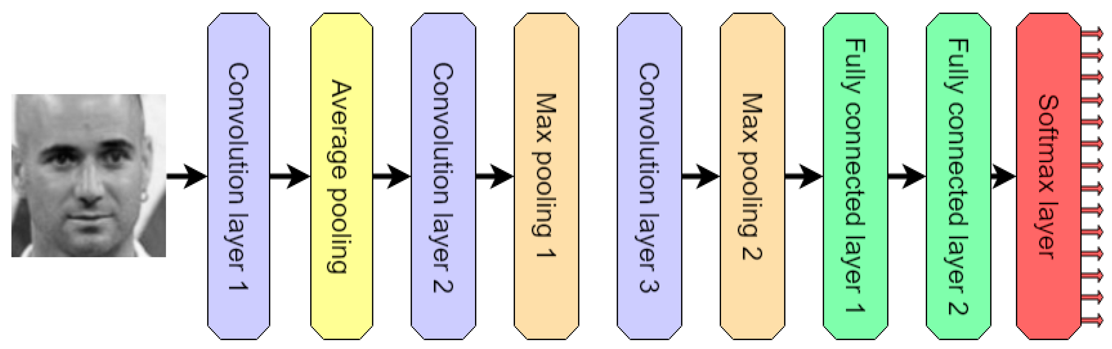
3.1.3. Discriminator

The proposed CNN structure for the discriminator consists of three convolutional layers, three pooling layers (two max-pooling and one average-pooling), two fully-connected layers and an output Softmax layer. The architecture is presented in Figure 6.

The input is represented by a 48 × 48 pixels grayscale image. Each of the three convolutional layers use 3 × 3 filter functions, with a stride of 1 and a padding of 1. The 0-padding was used to maintain the size of the output feature maps. The number of convolution filters increases from 32 (convolution layer 1) to 64 (convolution layer 2), and 128 (convolution layer 3), respectively. Each convolution layer is followed by a pooling layer. All three pooling layers which are used (one average-pooling and two max-pooling) have a stride size of 2 × 2 and dropouts of 0.1. The final two fully connected layers use 256 and 128 neurons, respectively, with dropouts of 0.4 and 0.5. The final layer of the proposed CNN is a Softmax layer with 14 possible outputs (7 emotion classes and real/fake classification).

The discriminator neural network was developed using Python and the machine learning framework, Tensorflow. It uses a new 2N output classes approach, by having a real and a fake class for each emotion. This approach helped improve the overall emotion classification by having the discriminator also trying to associate fake images with emotion classes of interest, instead of just rejecting the images as fake (N+1-classes approach).

3.1.4. Generator

The generator performs realistic facial expression synthesis. It receives a facial image that has to be modified, the target expression, and a sample facial image of the target expression, and then generates an image of the initial person with the expression of the second person, defined by the target emotion. The initial and generated images are 48 × 48 pixels grayscale images (R^{48 × 48}). Both the initial (I) and the label image (I_L) are processed by a four convolutional-layer network (encoder Enc_i), the initial image being mapped to a latent vector and the label image to a label vector, respectively. The concatenation result of the two vectors is used by a four deconvolutional-layer network (decoder-Dec) to generate the target image (Ĩ). The fully connected layer of the decoder learns the differences between the two vectors (latent-initial image and label-target/label image). The feedforward loop (FFL) is used to provide the raw features of the initial image (a down sampled version of the initial image), on which the differences identified by the first six layers of the decoder is applied. The formula for the obtained image is presented in Equation (4):

$$\mathsf{Ĩ}=Dec\left(En{c}_1\left(I\right),En{c}_2\left(I_L\right), FFL\right)$$

(4)

The description of the used layers is:

• Convolutional layers (1a–4a, 1b–4b)

  ○

  5 × 5 filter functions, stride 1, padding 2 (0-padding)

  ○

  Layers 1 and 2–128 neurons, Layers 3 and 4–256 neurons

• Max pooling layers (1a–4a, 1b–4b) with stride 2 × 2
• Fully connected layers

  ○

  256 neurons for the encoders, 512 for the decoder

• Deconvolutional (transposed convolution) layers (1–4)

  ○

  5 × 5 filter functions, stride 1, padding 2 (0-padding)

  ○

  Layers 1 and 2–128 neurons, Layers 3 and 4–256 neurons

• Upsampling layers (1–4) with stride 2 × 2
• Leaky ReLU as activation function—gradient 0.15

In most GAN implementation, a continuous noise vector is used to generate the images. The noise vector has no actual relevant information, but it is a source of randomness. By processing an initial image that has to be converted to a different facial expression, along with another image that has the desired facial expression, we construct a meaningful vector that is further used in the emotion-guided image generation process.

The generator neural network system was developed using Python and the machine learning framework, Tensorflow. The architecture is presented in Figure 7.

3.2. Operational Phase

After the proposed implementation in Figure 2 is trained and validated, several changes are made for the system to run independently. The classification part is the main component of the new system. There are three major changes from the proposed implementation in Figure 2. Firstly, the input image is provided by the user. The input image has to be a facial 48 × 48 pixels grayscale image. For the scope of this paper this is a mandatory requirement, but, for a future implementation, we consider adding another processing block so that the user can input a different size image and it will be converted to 48 × 48 pixels grayscale facial image. The second change is that the real and fake classes for each emotion are merged into a single class for each emotion. Both real and fake classes of the same emotions are considered to be the same class in this phase. This division was originally done during the training phase to increase the accuracy of the system. Thus only seven output classes remain. Finally, the feedback loop that was used to adjust the discriminator weights during supervised learning is removed, due to the fact that the images in this phase are not labeled. The new architecture for the classification system can be seen in Figure 8a. In order to reuse the generator, an additional system is proposed. The user can input a 48 × 48 pixels grayscale facial image and a target emotion for it, and the selected emotion will be transferred to the input image, changing the facial expression accordingly. The generator uses a random image belonging to the selected emotion class from the initial labeled dataset that was used for training. The proposed architecture for the generator system can be seen in Figure 8b.

4. Experimental Results

In order to train the proposed classification system we selected 7000 images (1000 images for each emotion class) from multiple datasets: LFW [48], FER 2013 [50], CK+ [53] and SFEW [54], FER+ [55]. Around 85% of the 7000 images used in this phase were selected from the FER 2013 dataset, which has the greatest diversity of the mentioned datasets, also being one of the largest open-source datasets for emotion recognition (almost 30,000 labeled images). The FER 2013 dataset consists of pre-cropped grayscale images of size 48 × 48, so all other selected images from different smaller datasets were manually cropped to have the same face pose and converted from RGB to grayscale. By using images from different datasets, we added an additional variety that the system had to handle. A selection of images for each emotion class can be seen in Figure 9.

The proposed system was implemented using Python and the Tensorflow machine learning framework. The algorithm was tested on system with 32GB DDR4 and a NVIDIA GeForce GTX 950M GPU with 4GB dedicated GDDR5 memory (NVIDIA Corporation, Santa Clara, CA, USA). For this setup we made use of the Tensorflow-CUDA (Compute Unified Device Architecture) toolkit integration, to enable parallel computing and obtain better execution times and performance. The system was trained for 200 epochs, when it was observed that the accuracy did not significantly improve anymore. Each epoch consisted of two sub-epochs. During the first sub-epoch, all 7000 test images are passed to the discriminator for classification (left side in Figure 2-I.). The image dataset was randomly split into two equal parts in sub-epoch 2 (right side in Figure 2-II). The first 3500 images were used to train the generator with the discriminator kept unchanged, while the next 3500 were used to test the discriminator with the generator unmodified. The batch size was 100 images in all scenarios, thus having 70 iterations for each sub-epoch and 140 iterations per epoch. The execution time averaged out at 6 hours per epoch (2 h for the first sub-epoch and 4 h for the second one).

In Figure 10, original, labeled and generated labeled images can be observed. These images are obtained using the right path in Figure 2-II (right side of Figure 2). After the training phase (200 epochs), a different set of 7000 images was selected from the FER 2013 dataset.

The proposed classification system was retested for another epoch using the new dataset. In

Table 1. Confusion matrix of the proposed system.

		Happiness (H)		Sadness (SA)		Anger (A)		Fear (FE)		Disgust (D)		Surprise (SU)		Neutral (N)
		R	F	R	F	R	F	R	F	R	F	R	F	R	F
H	R	911	37	0	0	0	0	0	0	0	0	19	7	21	5
	F	27	923	0	0	0	0	0	0	0	0	2	18	7	23
SA	R	6	0	704	62	19	3	9	0	55	9	3	0	97	33
	F	0	3	57	705	2	11	0	4	7	63	0	1	37	110
A	R	2	0	5	0	765	65	23	6	54	14	39	15	12	0
	F	0	1	0	2	92	771	5	17	12	50	14	25	2	9
FE	R	3	0	14	3	21	5	715	83	13	4	62	21	44	12
	F	0	0	4	10	5	10	89	719	2	7	19	61	13	51
D	R	2	0	15	4	67	20	15	4	753	82	9	3	21	5
	F	0	0	1	14	19	65	3	18	78	767	3	11	3	18
SU	R	78	28	0	0	3	0	58	15	13	3	712	85	5	0
	F	22	77	0	0	0	7	18	61	2	17	88	705	1	2
N	R	74	22	63	15	14	1	17	3	22	3	22	1	683	60
	F	12	76	10	52	0	12	1	18	4	21	2	32	64	696

, the confusion matrix obtained during the last epoch can be seen. For each emotion there were 2000 images, half real(R) and half generated (fake, F), like in each of the training epochs. The true positive entities were highlighted with gray.

In order to assess the performance of the proposed system we considered as a starting point the well-known statistical terminology:

• TP–Number of true positives, positive correctly classified as positive
• TN–Number of true negatives, negative correctly classified as negative
• FP–Number of false positives, negative classified as positive
• FN–Number of false negatives, positive classified as negative

We further compute statistical measures using the values described above. The measures and their formulas can be observed in

Table 2. Statistical measures of performance.

True positive rate (TPR)/sensitivity	$\frac{TP}{TP+FN}$	False positive rate (FPR)	$\frac{FP}{FP+TN}$
True negative rate (TNR)/specificity	$\frac{TN}{TN+FP}$	False negative rate (FNR)	$\frac{FN}{TP+FN}$
Positive prediction value (PPV)/precision	$\frac{TP}{TP+FP}$	False discovery rate (FDR)	$\frac{FP}{TP+FP}$
Negative prediction value (NPV)	$\frac{TN}{TN+FN}$	Accuracy (ACC)	$\frac{TP+TN}{TP+FP+TN+FN}$

:

For each emotion class, we compute the statistical measures in each of the following cases:

• Only real images of the class considered as positive (R)
• Only fake images of the class considered as positives (F)
• All images of the class (both real and fake) considered as positive (R + F)
• Real/fake differentiation (real images are positive, fake images are negative, regardless of the class) (R/F)

The results can be seen in

Table 3. Performance results.

		TPR	TNR	PPV	NPV	FPR	FNR	FDR	ACC
H	R	0.911	0.982	0.801	0.993	0.018	0.089	0.199	0.977
	F	0.923	0.981	0.791	0.994	0.019	0.077	0.209	0.977
	R + F	0.917	0.982	0.796	0.985	0.018	0.083	0.204	0.954
	R/F	0.951	0.964	0.963	0.951	0.036	0.049	0.037	0.9575
SA	R	0.704	0.987	0.806	0.977	0.013	0.296	0.194	0.966
	F	0.705	0.987	0.813	0.977	0.013	0.295	0.187	0.967
	R + F	0.704	0.987	0.809	0.951	0.013	0.296	0.191	0.934
	R/F	0.893	0.897	0.896	0.893	0.103	0.107	0.104	0.895
A	R	0.765	0.981	0.759	0.982	0.019	0.235	0.241	0.965
	F	0.771	0.984	0.794	0.982	0.016	0.229	0.206	0.969
	R + F	0.768	0.983	0.776	0.961	0.017	0.232	0.224	0.933
	R/F	0.900	0.875	0.878	0.897	0.125	0.100	0.122	0.887
FE	R	0.715	0.982	0.750	0.978	0.018	0.285	0.250	0.962
	F	0.719	0.982	0.758	0.978	0.018	0.281	0.242	0.963
	R + F	0.717	0.982	0.754	0.953	0.018	0.283	0.246	0.926
	R/F	0.872	0.869	0.868	0.87	0.131	0.128	0.132	0.865
D	R	0.753	0.980	0.741	0.980	0.020	0.247	0.259	0.963
	F	0.767	0.979	0.737	0.982	0.021	0.233	0.263	0.963
	R + F	0.760	0.979	0.739	0.958	0.021	0.240	0.261	0.927
	R/F	0.882	0.893	0.891	0.883	0.107	0.118	0.109	0.887
SU	R	0.712	0.978	0.716	0.977	0.022	0.288	0.284	0.959
	F	0.705	0.979	0.715	0.977	0.021	0.295	0.285	0.958
	R + F	0.709	0.978	0.716	0.951	0.022	0.291	0.284	0.918
	R/F	0.869	0.869	0.869	0.869	0.131	0.131	0.131	0.869
N	R	0.683	0.975	0.676	0.975	0.025	0.317	0.324	0.954
	F	0.696	0.975	0.679	0.976	0.025	0.304	0.321	0.954
	R + F	0.690	0.975	0.678	0.948	0.025	0.310	0.322	0.908
	R/F	0.895	0.907	0.905	0.896	0.093	0.105	0.095	0.901
Total	R	0.749	0.981	0.750	0.980	0.019	0.251	0.250	0.749
	F	0.755	0.981	0.754	0.981	0.019	0.245	0.246	0.755
	R + F	0.752	0.981	0.752	0.958	0.019	0.248	0.248	0.752
	R/F	0.894	0.896	0.895	0.894	0.104	0.106	0.105	0.829

, with the same notation for each emotion class as in Table 1.

The overall accuracy of the proposed system was 75.2%, while the accuracy of distinguishing between true and generated images was 82.9% (highlighted with gray). This final test was repeated, but this time without the generator module and the seven fake output classes, which were disabled. By doing this, we wanted to determine the improvement in accuracy brought by using the generator and the fake emotion classes. Only 7000 real images were used, and the obtained accuracy was 73.2%. Therefore, it was determined that adding the fake images in the classifications process contribute to a 2% increase in accuracy and variation of the tested images. There is no significant difference in accuracy between the tilted images and the front-faced images due to using the adjusting method presented in Section 3.1.2.

5. Discussion

A great variety of images (more than 14,000) from five different datasets (FER, FER+, LFW, CK+, SFEW) was used to test and validate the proposed system. The differences brought by gender, race, ethnicity, or age are minimized by computing the facial key points and the facial vectors from the center of gravity. By using this approach, we also handled the errors brought by tilted facial images, by adjusting the direction and magnitude of the facial vectors based on the face rotation. During the learning phase, the proposed CNN for emotion classification was tested both with real and generated images (thus increasing the variety to 28,000 images). Using the GAN approach to also generate images helps extend the available dataset and also introduces a greater variety of images. During each training epoch, the weights of the discriminator and generator are adjusted accordingly. This implementation increased the overall individual accuracy for each emotion class (R + F as opposed to R only), as can be seen in Table 3. It can be noted that the individual accuracy (class vs non-class) was quite high for each of the seven classes, ranging from 90% (neutral) to 97% (happiness). This variation can be explained by the fact that happiness was the only positive emotion we tested and can be easily distinguishable from the negative emotions. The lack of any emotion (neutral) was the closest to any emotion class and therefore more difficult to distinguish. Statistical comparison with similar works validated the proposed system, as observed in

Table 4. Accuracy (%) comparison for emotion classification.

Dataset	[46]	[49]	[50]	[52]	[55]	[56]	Our Method
FER 2013	-	94.7	71	73.4	63	66.7	75.2
CK+	-	-	-	99.1	-	98.4	98.3
SFEW	-	39	-	52	-	-	60.8
LFW	67.7	-	-	-	-	-	75.7
JAFFE	86.4	95.8	-	-	-	-	94.8

. In order to properly compare the results, we retested the algorithm for each distinct dataset (as opposed to the learning phase, where we used a selection of images from multiple datasets).

It can be observed that the accuracy of our system is among the highest for the FER 2013 dataset. The most notable accuracy obtained on FER 2013 dataset was 94.7, but it was obtained on a small subset of images (the authors from Reference [49] reported using 7% and 14% of the images in the FER 2013 dataset, while in the current research, we used almost 50% of the available images. The reported results were slightly better when comparing the 7% case, with an overall accuracy and accuracy for five emotions being better, with the 14% case, where accuracy for two emotion classes was better). Although the FER 2013 images represented a great percent of the images used in the learning phase, the system was able to properly classify images from the other used datasets, as shown by the obtained accuracies in each of the respective cases. Finally, we tested the system on a new dataset, JAFFE [47], which was not used at all during the learning phase. Due to using the image processing block (facial points detection and post-processing) to minimize image variations, the system was able to correctly classify the new images with a high accuracy (94.8%).

6. Conclusions and Further Work

The proposed method, based on a Generative Adversarial Network, for emotion detection improved the classification accuracy for five combined facial dataset (75.2%—the overall accuracy, and 82.9%—the accuracy of identification true/generated images). The obtained system (operational phase) was flexible, allowing the use of images with great differences (gender, age, and race) as inputs. Moreover, the generator could be used as a standalone component for emotion change in any image. In order to reduce the calculus volume, the rotation-invariant facial points were used as inputs for the classifier of seven emotions.

One future research direction is represented by trying to identify a correlation between the emotions expressed by different individuals over a period of time and the evolution of their health state. This kind of study implies monitoring the persons at random intervals in their natural state using their smartphone, laptop, or smart TV camera and finding their predominant emotion in different situations throughout the day. The study is guided by the idea that a negative emotion can have impact on the overall health state, leading to stress and ultimately to diseases like cancer [32,33,34,35]. A strong collaboration with a medical institute is planned.

Another research direction is represented by the possibility to monitor and evaluate the emotion caused by different advertising campaigns (photos or videos) using the smartphone camera. In this way we can assess how well the campaign is received by the public.

References

1. Wiskott, L.; Kruger, N.; Von Der Malsburg, C. Face recognition by elastic bunch graph matching. IEEE Trans. Pattern Anal. Mach. Intell. 1997, 19, 775–779. [Google Scholar] [CrossRef] [Green Version]
2. Face Recognition Market by Component, Technology, Use Case, End-User, and Region–Global Forecast to 2022. Available online: https://www.marketsandmarkets.com/Market-Reports/facial-recognition-market-995.html (accessed on 21 March 2018).
3. Yang, M.H.; Kriegman, D.J.; Ahuja, N. Detecting Faces in Images: A survey. IEEE Trans. Pattern Anal. Mach. Intell. 2002, 19, 775–779. [Google Scholar]
4. Gupta, V.; Sharma, D. A study of various face detection methods. Int. J. Adv. Res. Comput. Commun. Eng. 2014, 3, 6694–6697. [Google Scholar]
5. Hiyam, H.; Beiji, Z.; Majeed, R. A survey of feature base methods for human face detection. Int. J. Control Autom. 2015, 8, 61–77. [Google Scholar]
6. Smrti, T.; Nitin, M. Detection, segmentation and recognition of face and its features using neural network. J. Biosens. Bioelectron. 2016, 7. [Google Scholar] [CrossRef]
7. Le, T.H. Applying Artificial Neural Networks for Face Recognition. Adv. Artif. Neural Syst. 2011. [Google Scholar] [CrossRef]
8. Farfade, S.S.; Saberian, M.; Li, L.J. Multiview face detection using deep convolutional neural networks. In Proceedings of the 5th International Conference on Multimedia Retrieval (ICMR), Shanghai, China, 23–26 June 2015. [Google Scholar]
9. Martinez-Gonzalez, A.N.; Ayala-Ramirez, V. Real time face detection using neural networks. In Proceedings of the 10th Mexican International Conference on Artificial Intelligence, Puebla, Mexico, 26 November–4 December 2011. [Google Scholar]
10. Kasar, M.M.; Bhattacharyya, D.; Kim, T.H. Face recognition using neural network: A review. Int. J. Secur. Appl. 2016, 10, 81–100. [Google Scholar] [CrossRef]
11. Al-Allaf, O.N. Review of face detection systems based artificial neural networks algorithms. Int. J. Multimed. Appl. 2014, 6. [Google Scholar] [CrossRef]
12. Prihasto, B.; Choirunnisa, S.; Nurdiansyah, M.I.; Mathulapragsan, S.; Chu, V.C.; Chen, S.H.; Wang, J.C. A survey of deep face recognition in the wild. In Proceedings of the 2016 International Conference on Orange Technologies, Melbourne, Australia, 17–20 December 2016. [Google Scholar] [CrossRef]
13. Fu, Z.P.; Zhang, Y.N.; Hou, H.Y. Survey of deep learning in face recognition. In Proceedings of the 2014 International Conference on Orange Technologies, Xi’an, China, 20–23 September 2014. [Google Scholar] [CrossRef]
14. Wang, M.; Deng, W. Deep face recognition: A survey. arXiv, 2018; arXiv:1804.06655. [Google Scholar]
15. Kim, Y.G.; Lee, W.O.; Kim, K.W.; Hong, H.G.; Park, K.R. Performance enhancement of face recognition in smart TV using symmetrical fuzzy-based quality assessment. Symmetry 2015, 7, 1475–1518. [Google Scholar] [CrossRef]
16. Hong, H.G.; Lee, W.O.; Kim, Y.G.; Kim, K.W.; Nguyen, D.T.; Park, K.R. Fuzzy system-based face detection robust to in-plane rotation based on symmetrical characteristics of a face. Symmetry 2016, 8, 75. [Google Scholar] [CrossRef]
17. Sharifi, O.; Eskandari, M. Cosmetic Detection framework for face and iris biometrics. Symmetry 2018, 10, 122. [Google Scholar] [CrossRef]
18. Li, Y.; Song, L.; He, R.; Tan, T. Anti-Makeup: Learning a bi-level adversarial network for makeup-invariant face verification. arXiv, 2018; arXiv:1709.03654. [Google Scholar]
19. Goodfellow, I.J.; Pouget-Abadie, J.; Mirza, M.; Xu, B.; Warde-Farley, D.; Ozair, S.; Courville, A.; Bengio, Y. Generative Adversial Nets. arXiv, 2014; arXiv:1406.2661. [Google Scholar]
20. Odena, A.; Olah, C.; Shlens, J. Conditional Image Synthesis with Auxiliary Classifier GANs. arXiv, 2016; arXiv:1610.09585. [Google Scholar]
21. Gauthier, J. Conditional Generative Adversarial Nets for Convolutional Face Generation. 2015. Available online: http://cs231n.stanford.edu/reports/2015/pdfs/jgauthie_final_report.pdf (accessed on 15 April 2018).
22. Antipov, G.; Baccouche, M.; Dugelay, J.L. Face aging with conditional generative adversarial networks. arXiv, 2017; arXiv:1702.01983. [Google Scholar]
23. Huang, E.; Zhang, S.; Li, T.; He, R. Beyond face rotation: Global and local perception gan for photorealistic and identity preserving frontal view synthesis. arXiv, 2017; arXiv:1704.04086. [Google Scholar]
24. Li, Z.; Luo, Y. Generate identity-preserving faces by generative adversarial networks. arXiv, 2017; arXiv:1706.03227. [Google Scholar]
25. Zhou, H.; Sun, J.; Yacoob, Y.; Jacobs, D.W. Label Denoising Adversarial Network (LDAN) for Inverse Lighting of Face Images. arXiv, 2017; arXiv:1709.01993. [Google Scholar]
26. Zhang, W.; Shu, Z.; Samaras, D.; Chen, L. Improving heterogeneous face recognition with conditional adversial networks. arXiv, 2017; arXiv:1709.02848. [Google Scholar]
27. Springenberg, J.T. Unsupervised and semi-supervised learning with categorical generative adversarial networks. arXiv, 2015; arXiv:1511.06390. [Google Scholar]
28. Radford, A.; Metz, L.; Chintala, S. Unsupervised representation learning with deep convolutional generative adversarial networks. arXiv, 2015; arXiv:1511.06434. [Google Scholar]
29. Odena, A. Semi-supervised learning with generative adversarial networks. arXiv, 2016; arXiv:1606.01583. [Google Scholar]
30. Salimans, T.; Goodfellow, I.; Zaremba, W.; Cheung, V.; Radford, A.; Chen, X. Improved techniques for training Gans. arXiv, 2016; arXiv:1606.03498. [Google Scholar]
31. Papernot, N.; Abadi, M.; Erlingsson, U.; Goodfellow, I.; Talwar, K. Semi-supervised knowledge transfer for deep learning from private training data. arXiv, 2016; arXiv:1610.05755. [Google Scholar]
32. Fredrickson, B.L. Cultivating positive emotions to optimize health and well-being. Prev. Treat. 2003, 3. [Google Scholar] [CrossRef]
33. Fredrickson, B.L.; Levenson, R.W. Positive emotions speed recovery from the cardiovascular sequelae of negative emotions. Cogn. Emot. 1998, 12, 191–220. [Google Scholar] [CrossRef] [PubMed]
34. Gallo, L.C.; Matthews, K.A. Understanding the association between socioeconomic status and physical health: Do negative emotions play a role? Psychol. Bull. 2003, 129, 10–51. [Google Scholar] [CrossRef] [PubMed] [Green Version]
35. Todaro, J.F.; Shen, B.J.; Niura, R.; Sprio, A.; Ward, K.D. Effect of negative emotions on frequency of coronary heart disease (The Normative Aging Study). Am. J. Cardiol. 2003, 92, 901–906. [Google Scholar] [CrossRef]
36. Huang, Y.; Khan, S.M. DyadGAN: Generating facial expressions in dyadic interactions. In Proceedings of the IEEE Conference on Computer Vision and Pattern Recognition Workshops, Honolulu, HI, USA, 21–26 July 2017. [Google Scholar] [CrossRef]
37. Zhou, Y.; Shi, B.E. Photorealistic facial expression synthesis by the conditional difference adversarial autoencoder. arXiv, 2017; arXiv:1708.09126. [Google Scholar] [Green Version]
38. Lu, Y.; Tai, Y.W.; Tang, C.K. Conditional CycleGAN for attribute guided face image generation. arXiv, 2017; arXiv:1705.09966. [Google Scholar]
39. Ding, H.; Sricharan, K.; Chellappa, R. ExprGAN: Facial expression editing with controllable expression intensity. arXiv, 2017; arXiv:1709.03842. [Google Scholar]
40. Xu, R.; Zhou, Z.; Zhang, W.; Yu, Y. Face transfer with generative adversarial network. arXiv, 2017; arXiv:1710.06090. [Google Scholar]
41. Nojavanasghari, B.; Huang, Y.; Khan, S.M. Interactive generative adversarial networks for facial expression generation in dyadic interactions. arXiv, 2018; arXiv:1801.09092. [Google Scholar]
42. Tian, Y.L.; Kanage, T.; Cohn, J. Robust Lip Tracking by Combining Shape, Color and Motion. In Proceedings of the 4th Asian Conference on Computer Vision, Taipei, Taiwan, 8–11 January 2000. [Google Scholar]
43. Agarwal, M.; Krohn-Grimberghe, A.; Vyas, R. Facial key points detection using deep convolutional neural network—Naimishnet. arXiv, 2017; arXiv:1710.00977. [Google Scholar]
44. Kazemi, V.; Sullivan, J. One millisecond face alignment with an ensemble of regression trees. In Proceedings of the 2014 IEEE Conference on Computer Vision and Pattern Recognition, Columbus, OH, USA, 23–28 June 2014. [Google Scholar] [CrossRef]
45. Suh, K.H.; Kim, Y.; Lee, E.C. Facial feature movements caused by various emotions: Differences according to sex. Symmetry 2016, 8, 86. [Google Scholar] [CrossRef]
46. Dachapally, P.R. Facial emotion detection using convolutional neural networks and representational autoencoder units. arXiv, 2017; arXiv:1706.01509. [Google Scholar]
47. Lyons, M.J.; Kamachi, M.; Gyoba, J. Japanese Female Facial Expressions (JAFFE). Database of Digital Images. 1997. Available online: http://www.kasrl.org/jaffe.html (accessed on 15 April 2018).
48. Huang, G.B.; Ramesh, M.; Berg, T.; Learned-Miller, E. Labeled Faces in the Wild: A Database for Studying Face Recognition in Unconstrained Environments; Workshop on Faces in ’RealLife’ Images: Detection, Alignment, and Recognition: Marseille, France, 2008. [Google Scholar]
49. Zhu, X.; Liu, Y.; Qin, Z.; Li, J. Data augmentation in emotion classification using generative adversarial networks. arXiv, 2017; arXiv:1711.00648. [Google Scholar]
50. Facial Expression Recognition (FER2013) Dataset. Available online: https://www.kaggle.com/c/challenges-in-representation-learning-facial-expression-recognition-challenge/data (accessed on 19 October 2017).
51. Lee, K.W.; Hong, H.G.; Park, K.R. Fuzzy system-based fear estimation based on the symmetrical characteristics of face and facial feature points. Symmetry 2017, 9, 102. [Google Scholar] [CrossRef]
52. Al-Shabi, M.; Cheah, W.P.; Connie, T. Facial expression recognition using a hybrid CNN-SIFT aggregator. arXiv, 2016; arXiv:1608.02833. [Google Scholar]
53. Lucey, P.; Cohn, J.F.; Kanade, T.; Saragih, J.; Ambadar, Z.; Matthews, I. The Extended Cohn-Kanade Dataset (CK+); A Complete Dataset for Action Unit and Emotion-Specified Expression. In Proceedings of the 2010 IEEE Computer Society Conference on Computer Vision and Pattern Recognition Workshops, San Francisco, CA, USA, 13–18 June 2010. [Google Scholar]
54. Dhal, A.; Goecke, R.; Luvey, S.; Gedeon, T. Static facial expressions in tough; data, evaluation protocol and benchmark. In Proceedings of the IEEE International Conference on Computer Vision ICCV2011, Barcelona, Spain, 6–13 November 2011. [Google Scholar]
55. Mishra, S.; Prasada, G.R.B.; Kumar, R.K.; Sanyal, G. Emotion Recognition through facila gestures—A deep learning approach. In Proceedings of the Fifth International Conference on Mining Intelligence and Knowledge Exploration (MIKE), Hyderabad, India, 13–15 December 2017; pp. 11–21. [Google Scholar]
56. Quinn, M.A.; Sivesind, G.; Reis, G. Real-Time Emotion Recognition from Facial Expressions. 2017. Available online: http://cs229.stanford.edu/proj2017/final-reports/5243420.pdf (accessed on 15 April 2018).
57. Plutschik, R. The nature of emotions. Am. Sci. 2001, 89, 344. [Google Scholar] [CrossRef]
58. Chen, X.; Duan, Y.; Houthooft, R.; Schulman, J.; Sutskever, I.; Abbeel, P. InfoGAN: Interpretable Representation Learning by Information Maximizing Generative Adversarial Nets. arXiv, 2016; arXiv:1606.03657. [Google Scholar]
59. Dlib Library. Available online: http://blog.dlib.net/2014/08/real-time-face-pose-estimation.html (accessed on 12 November 2017).
Figure 1. Different GAN (generative adversarial network) implementations: (a) Conditional GAN [19]; (b) Semi-Supervised GAN [29]; (c) Info-GAN [58].
Symmetry 10 00414 g001
Figure 2. Proposed GAN architecture.
Symmetry 10 00414 g002
Figure 3. Images resulted from dlib detector (a) 68 points; (b) Initial image with facial key points; (c) 51 extracted facial key points.
Symmetry 10 00414 g003
Figure 4. Center of gravity and connections with facial key points.
Symmetry 10 00414 g004
Figure 5. Computing the offset to correct face tilt.
Symmetry 10 00414 g005
Figure 6. Discriminator architecture.
Symmetry 10 00414 g006
Figure 7. Generator architecture.
Symmetry 10 00414 g007
Figure 8. Discriminator and generator adapted for the operational phase: (a) Discriminator; (b) Generator.
Symmetry 10 00414 g008
Figure 9. Sample images from the selected datasets.
Symmetry 10 00414 g009
Figure 10. Generator results.
Symmetry 10 00414 g010