Article

A Dynamic Adjusting Novel Global Harmony Search for Continuous Optimization Problems

1
Industrial Engineering and Management, National Taipei University of Technology, Taipei 10632, Taiwan
2
College of Management, National Taipei University of Technology, Taipei 10632, Taiwan
3
Department of Computer Science, Concordia University Chicago, Chicago, IL 60305, USA
*
Author to whom correspondence should be addressed.
Symmetry 2018, 10(8), 337; https://doi.org/10.3390/sym10080337
Submission received: 10 July 2018 / Revised: 6 August 2018 / Accepted: 8 August 2018 / Published: 12 August 2018
(This article belongs to the Special Issue Information Technology and Its Applications 2021)

Abstract

:
A novel global harmony search (NGHS) algorithm, as proposed in 2010, is an improved algorithm that combines the harmony search (HS), particle swarm optimization (PSO), and a genetic algorithm (GA). Moreover, the fixed parameter of mutation probability was used in the NGHS algorithm. However, appropriate parameters can enhance the searching ability of a metaheuristic algorithm, and their importance has been described in many studies. Inspired by the adjustment strategy of the improved harmony search (IHS) algorithm, a dynamic adjusting novel global harmony search (DANGHS) algorithm, which combines NGHS and dynamic adjustment strategies for genetic mutation probability, is introduced in this paper. Moreover, extensive computational experiments and comparisons are carried out for 14 benchmark continuous optimization problems. The results show that the proposed DANGHS algorithm has better performance in comparison with other HS algorithms in most problems. In addition, the proposed algorithm is more efficient than previous methods. Finally, different strategies are suitable for different situations. Among these strategies, the most interesting and exciting strategy is the periodic dynamic adjustment strategy. For a specific problem, the periodic dynamic adjustment strategy could have better performance in comparison with other decreasing or increasing strategies. These results inspire us to further investigate this kind of periodic dynamic adjustment strategy in future experiments.

1. Introduction

The last two decades have seen a significant increase in research into metaheuristic algorithms. The procedure of a metaheuristic algorithm can be divided into four steps: initialization, movement, replacement, and iteration [1]. The most popular metaheuristic algorithms to date are the particle swarm optimization (PSO) [2,3], genetic algorithm (GA) [4,5,6], and ant colony optimization (ACO) [7,8,9].
PSO was introduced by Kennedy and Eberhart in 1995 [10,11]. It imitates the foraging behavior of birds and fish, and provides a population-based search procedure, where each individual is abstracted as a “particle” that flies around in a multidimensional search space. The best positions encountered by a particle and its neighbors determine the particle’s trajectory, along with other PSO parameters. In other words, a PSO system attempts to balance exploration and exploitation by combining global and local search methods [12].
The GA has been widely investigated since Holland proposed it in 1960 [13,14]. The GA was developed from Darwinian evolution. Based on the concept of natural genetics and evolutionary principles, GA is a stochastic search technique that can search the near optimum solution in a large and complicated space. As Gordini [15] points out, “the GA differs from other non-linear optimization techniques in that it searches by maintaining a population of solutions from which better solutions are created, rather than making incremental changes to a single solution to a problem.” The GA is consisted of three operators: reproduction, crossover, and mutation [16]. Reproduction is a process of survival-of-the-fittest selection. Crossover is the partial swap between two parent strings in order to produce two offspring strings. Mutation is the occasional random inversion of bit values in order to generate a non-recursive offspring. One importance of the GA is that several metaheuristic algorithms have been developed from the GA, such as the honey-bee mating optimization (HBMO) algorithm [17] and the harmony search (HS) algorithm [16].
The harmony search (HS) algorithm is a modern metaheuristic intelligent evolution algorithm [18], and was inspired by the music improvisation process where musicians improvise their instruments’ pitches searching for a perfect state of harmony [19]. The HS algorithm simulates the principle of the music improvisation process in the same way that the GA simulates biological evolution, the simulated annealing algorithm (SA) [20] simulates physical annealing, and the PSO algorithm simulates the swarm behavior of birds and fish [18], etc. The HS algorithm has excellent exploitation capabilities. However, the HS algorithm suffers a very serious limitation of premature convergence if one or more initially generated harmonies are in the vicinity of local optimal [21]. As Assad and Deep [22] point out, “The efficiency of evolutionary algorithms depends on the extent of balance between diversification and intensification during the course of the search. Intensification, also called exploitation, is the ability of an algorithm to exploit the search space in the vicinity of the current good solution, whereas diversification, also called exploration, is the process of exploring the new regions of a large search space and thus allows dissemination of the new information into the population. Proper balance between these two contradicting characteristics is a must to enhance the performance of the algorithm.”
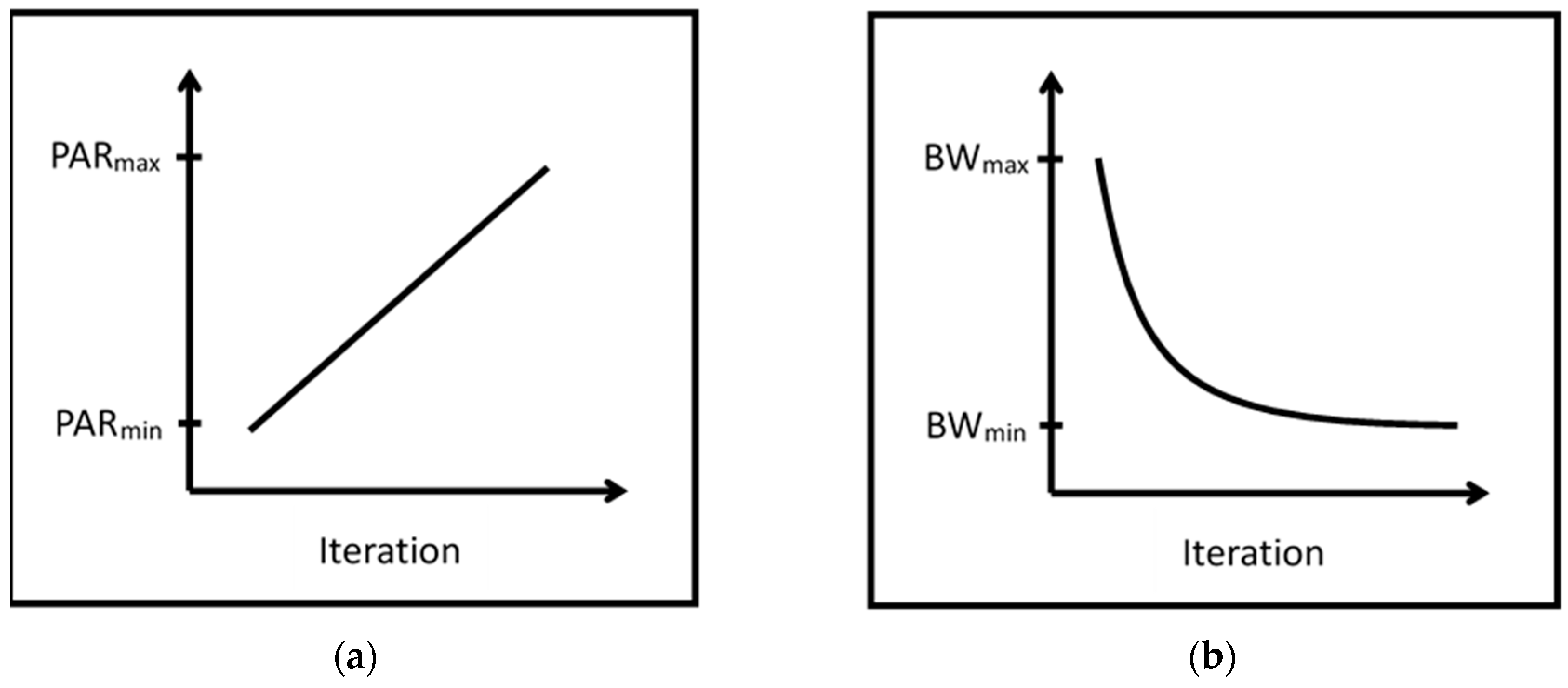
Therefore, in order to eradicate the aforementioned limitation, several improved HS algorithms have been proposed, such as the improved harmony search (IHS) algorithm [23], the self-adaptive global best harmony search (SHGS) [24], the novel global harmony search (NGHS) [25], the intelligent global harmony search (IGHS) algorithm [19], and so on. Of these algorithms, the IHS algorithm is the first to propose using the adjustment strategy to tune the pitch adjusting rate (PAR) and bandwidth (BW) parameters. In the HS algorithm, according to the value of PAR, the musicians will determine to adjust their instruments’ pitches or not. Besides, the musicians will adjust the pitches within the BW distance. The PAR and BW values change dynamically with generation number, as shown in Figure 1. In Mahdavi’s paper [23], the adjustment strategy was proofed; it can enhance the searching ability of the harmony search algorithm. In other words, the importance of the appropriate parameters was proofed in his paper.
Appropriate parameters can enhance the searching ability of a metaheuristic algorithm; their importance has been described in many studies. First, Pan et al. demonstrated that a good set of parameters can enhance an algorithm’s ability to search for the global optimum or near optimum region with a high convergence rate [19,24]. Second, in the NGHS algorithm, the new trial solutions are generated by the parameter s t e p j . Therefore, Zou et al. [25,26] showed that the most reasonable design for s t e p j in the NGHS algorithm can guarantee that the proposed algorithm has strong global search ability in the early optimization stage, and strong local search ability in the late optimization stage. In addition, a dynamically adjusted s t e p j maintains a balance between the global search and the local search. In another paper, Zou et al. [27] demonstrated that an appropriate harmony memory considering rate (HMCR) and PAR value in the SGHS algorithm can be gradually learned to suit the particular problem and the particular phases of the search process. In addition, there is no single choice for the genetic mutation probability ( p m ) in the NGHS algorithm; it should be adjusted according to practical optimization problems. Last, Valian, Tavakoli, and Mohanna [28] observed that there can be no single choice for HMCR in the IGHS algorithm, and it should be adjusted according to the given optimization problems.
However, in the NGHS algorithm, the value of the genetic mutation probability ( p m ) is a fixed value that is given in the initialization step. According to the result of Mahdavi’s paper [23], we supposed that the adjustment strategy could enhance the searching ability. Therefore, a dynamic adjusting novel global harmony search (DANGHS) algorithm was proposed in this paper. In the DANGHS algorithm, the mutation probability adjusts dynamically with the generation number by the adjustment strategy. However, we can adjust the mutation probability using different strategies. Therefore, this paper used 16 different strategies in the DANGHS algorithm in 14 well-known benchmark optimization problems. In other words, the performance of different strategies in the DANGHS algorithm for different problems was investigated. Besides, in general, one important characteristic of the metaheuristic algorithm is to be fast and efficient. A better metaheuristic algorithm cannot only search the more exact solution but also use less iterations than other algorithms. Therefore, we discuss the efficiency of the DANGHS algorithm in this paper. According to the numerical results, the DANGHS algorithm had better searching performance in comparison with other HS algorithms in most problems.
The remainder of this paper is arranged as follows. In Section 2, the HS, IHS, SGHS, and NGHS algorithms are introduced. Section 3 describes the DANGHS algorithm. A large number of experiments are carried out to test and compare the performance of 16 different strategies in the DANGHS algorithm in Section 4. Conclusions and suggestions for future research are given in Section 5.

2. HS, IHS, SGHS, and NGHS

In this section, the HS, the IHS, the SGHS, and the NGHS are reviewed.

2.1. Harmony Search Algorithm

The HS algorithm was proposed by Geem, Kim, and Loganathan in 2001 [16]. HS is similar in concept to other metaheuristic algorithms such as GA, PSO, and ACO in terms of combining the rules of randomness to imitate the process that inspired it. However, HS draws its inspiration not from biological or physical processes but from the improvisation process of musicians, such as that found in a Jazz trio [19,29].
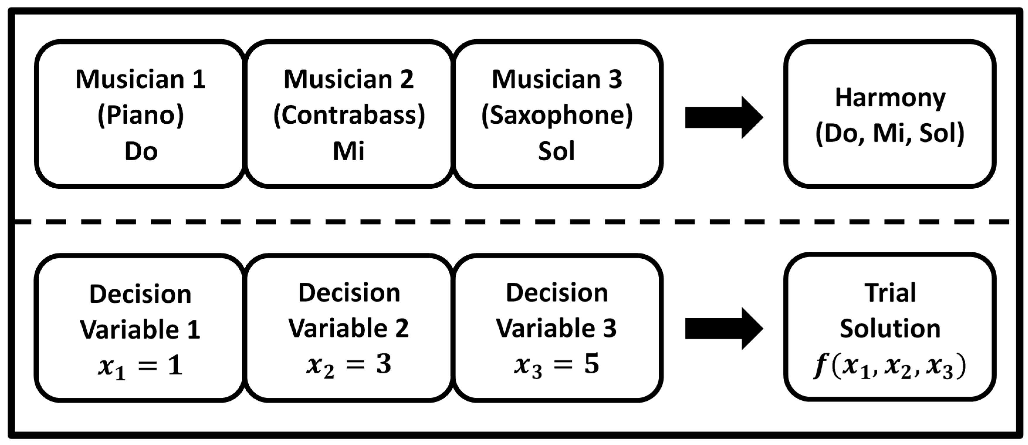
In the musical improvisation process, each musician sounds any pitch within a possible range, and then together they make a single harmony. If all the pitches make a pleasing harmony, the experience is stored in each player’s memory, and the possibility of making a more pleasing harmony the next time is increased [30]. Similarly, in engineering optimization, each decision variable initially chooses any value within a possible range, together making one solution vector [27]. In the HS algorithm, each harmony, which means the trial solution for the problem, is represented by a D-dimension real vector, and a pleasing harmony means the good trial solution for the problem [19]. If all the decision variable values make a good solution, then that experience is stored in each variable’s memory, and the possibility of making a good solution the next time is also increased [27]. Figure 2 shows the comparison between music improvisation and engineering optimization. In Figure 2, there is a Jazz trio consisting of three musicians. Each musician plays an instrument at the same time to make a single harmony. The pitches of the three instruments mean the values of the three decision variables.
In general, the HS algorithm works as follows [27]:
Step 1. Initialization: the algorithm and problem parameters
In this step, the parameters of the HS algorithm are determined. The parameters are the harmony memory size (m), the harmony memory considering rate (HMCR), the pitch adjusting rate (PAR), the bandwidth (BW), the current iteration (k = 1), and the maximum number of iterations (NI). Furthermore, the D-dimensional optimization problem is defined as Minimize f(x) subject to x j L x j x j U   ( j = 1 ,   2 ,   ,   D ) . x j L and x j U are the lower and upper bounds for decision variables x j .
Step 2. Initialization: the decision variable values and the harmony memory
The initial decision variable values x i j k = 0 ( i = 1 ,   2 ,   ,   m ) are generated by Equation (1). The harmony memory (HM) is as shown in Equation (2).
x i j 0 = x j L + r × ( x j U x j L )
HM = [ x 11 0 x 12 0 x 21 0 x 22 0 x 1 D 0 x 2 D 0 x m 1 0 x m 2 0 x m D 0 ]
In Equation (1), r is the uniformly generated random numbers in the region of [0, 1].
Step 3. Movement: improvise a new harmony
Movement step is the most important step of any algorithm. The performance of global exploration and local exploitation are related to the design of the movement step. In the HS algorithm, the movement step is improvisation. The new harmony vector x k + 1 = ( x 1 k + 1 , x 2 k + 1 , , x D k + 1 ) is generated by memory consideration, pitch adjustment, and random selection mechanisms in this step. The HS movement steps (Pseudocode 1) are shown in Algorithm 1.
Algorithm 1 The Movement Steps of HS (Pseudocode 1)
1:For j = 1   to   D do
2:  If r 1 H M C R then
3:    x j k + 1 = x i j k  % memory consideration
4:   If r 2 P A R then
5:     x j k + 1 = x j k + 1 B W + r 3 × 2 × B W  % pitch adjustment
6:    If x j k + 1 > x j U then
7:      x j k + 1 = x i U
8:    Else if x j k + 1 < x j L then
9:      x j k + 1 = x i L
10:    End
11:   End
12:  Else
13:    x j k + 1 = x j L + r 4 × ( x j U x j L )  % random selection
14:  End
15:End
Here, x j k + 1 is the jth component of x k + 1 . i is an uniformly generated random number in [1, m], and x i j k is the jth component of the ith candidate solution vector in the HM. r 1 , r 2 , r 3 and r 4 are the uniformly generated random numbers in the region of [0, 1], and BW is a given distance bandwidth.
Step 4. Replacement: update harmony memory
If the fitness value of the new harmony vector x k + 1 is better than that of the worst harmony in the HM, replace the worst harmony vector by x k + 1 .
Step 5. Iteration: check the stopping criterion
If the stopping criterion (maximum number of iterations NI) is satisfied, the computation is terminated; otherwise, the current iteration k = k + 1 and go back to step 3.

2.2. Improved Harmony Search Algorithm

The IHS algorithm was proposed by Mahdavi, Fesanghary, and Damangir in 2007 for solving optimization problems [23]. In their paper, they noted that PAR and BW are very important parameters in the HS algorithm when fine-tuning optimized solution vectors, and can be potentially useful in adjusting the convergence rate of the algorithm to the optimal solution. Fine adjustment of these parameters is therefore of particular interest. The key difference between the IHS and the traditional HS method is thus in the way PAR and BW are adjusted in each iteration by Equations (3) and (4):
P A R k = P A R m i n + ( P A R m a x P A R m i n ) N I × k
B W k = B W m a x × e ( ln ( B W m i n B W m a x ) × k / N I )
In Equation (3), P A R k is the pitch adjustment rate in the current iteration k; P A R m i n and P A R m a x are the minimum and maximum adjustment rates, respectively. In Equation (4), B W k is the distance bandwidth in current iteration k, B W m i n is the minimum bandwidth, and B W m a x is the maximum bandwidth. Figure 1 shows that the PAR and BW values change dynamically with the iteration number.

2.3. Self-Adaptive Global Best Harmony Search Algorithm

The SGHS algorithm was presented by Pan et al. in 2010 for continuous optimization problems [24].
In the SGHS algorithm, the HMCR and PAR were dynamically adapted by the normal distribution and the BW was adjusted in each iteration. The value of H M C R k was generated by the mean H M C R m and the standard deviation. In the same way, the value of P A R k was generated by the mean P A R m and the standard deviation. Pan et al. assumed that the dynamic mean H M C R m is in the range of [0.9, 1.0] and the static standard deviation is 0.01; the dynamic mean P A R m . is in the range of [0.0, 1.0] and the static standard deviation is 0.05. Furthermore, the H M C R k and P A R k were recorded by their historic values when the generated harmony successfully replaced the worst harmony in the harmony memory. After a specified learning period (LP), the H M C R m and P A R m were recalculated by averaging all the recorded H M C R k and P A R k values during this period respectively. In the subsequent iterations, new H M C R k and P A R k values were generated with the new mean H M C R m and P A R m and the given standard deviation. In addition, the B W k is decreased in each iteration by Equation (5).
B W k = { B W m a x B W m a x B W m i n N I × 2 k i f   k < N I / 2 , B W m i n i f   k N I / 2 ,
In general, the SGHS algorithm works as follows:
Step 1. Initialization: the problem and algorithm parameters
Set parameters m, LP, NI, B W m a x , B W m i n , H M C R m , P A R m , the current iteration k = 1, and iteration counter lp = 1.
Step 2. Initialization: the decision variable values and the harmony memory
The initial decision variable values x i j k = 0 ( i = 1 ,   2 ,   ,   m ) is generated by Equation (1). The harmony memory (HM) is as shown in Equation (2).
Step 3. Movement: generate the algorithm parameters
Generate H M C R k and P A R k with H M C R m and P A R m by the normal distribution respectively. Generate B W k with B W m a x and B W m i n by Equation (5).
Step 4. Movement: improvise a new harmony
Improvise a new harmony x k + 1 . The SGHS movement step (Pseudocode 2) is shown in Algorithm 2.
Algorithm 2 The Movement Steps of SGHS (Pseudocode 2) [24]
1:For j = 1   to   D do
2:  If r 1 HMCR k then
3:    x j k + 1 = x i j k B W k + r 2 × 2 × B W k
4:   If x j k + 1 > x j U then
5:     x j k + 1 = x i U
6:   Else if x j k + 1 < x j L then
7:     x j k + 1 = x i L
8:   End
9:   If r 3 PAR k then
10:     x j k + 1 = x b e s t , j k
11:   End
12:  Else
13:    x j k + 1 = x j L + r 4 × ( x j U x j L )  % random selection
14:  End
15:End
Here, x j k + 1 is the jth component of x k + 1 . i is an uniformly generated random number in [1, m], and x i j k is the jth component of the ith candidate solution vector in the HM. x b e s t , j k is the jth component of the best candidate solution vector in the HM. r 1 , r 2 , r 3 and r 4 are uniformly generated random numbers in [0, 1]. r 1 is used for position updating, r 2 determines the distance of the BW, r 3 is used for pitch adjustment, and r 4 is used for random selection.
Step 5. Replacement: update harmony memory
If the fitness value of the new harmony vector x k + 1 is better than that of the worst harmony in the HM, replace the worst harmony vector by x k + 1 and record the values of H M C R k and P A R k .
Step 6. Replacement: update H M C R m and P A R m
If lp = LP, recalculate H M C R m and P A R m by averaging all the recorded H M C R k and P A R k values respectively and reset lp = 1; otherwise, lp = lp +1.
Step 7. Iteration: check the stopping criterion
If NI is completed, return the best harmony vector x b e s t in the HM; otherwise, the current iteration k = k + 1 and go back to step 3.

2.4. Novel Global Harmony Search Algorithm

The NGHS algorithm [25,26] is an improved algorithm that combines HS, PSO, and GA. A prominent characteristic of PSO is that individual particles attempt to imitate the social experience. It means the particles are affected by other better particles in the PSO algorithm. A prominent characteristic of GA is that it is possible for the trial solution to escape from the local optimum by mutation. In other words, NGHS tries to generate a new solution by moving the worst solution toward the best solution or by mutation.
Figure 3 is used to illustrate the principle of position updating. s t e p j = | x b e s t , j k x w o r s t , j k | is defined as an adaptive step of the jth decision variable. This adaptive step can dynamically balance the performance of global exploration and local exploitation in the NGHS algorithm. As Zou et al. [26] points out, “In the early stage of optimization, all solution vectors are sporadic in the solution space, so most adaptive steps are large, and most trust regions are wide, which is beneficial to the global search of NGHS. However, in the late stage of optimization, all non-best solution vectors are inclined to move to the global best solution vector, so most solution vectors are close to each other. In this case, most adaptive steps are small and most trust regions are narrow, which is beneficial to the local search of NGHS.”
According to this prominent characteristic, NGHS modifies the movement step of HS therefore the NGHS algorithm can imitate the current best harmony in the HM. In general, the NGHS algorithm works as follows:
Step 1. Initialization: the algorithm and problem parameters
(1)
Set parameters m, NI, and the current iteration k = 1.
(2)
The genetic mutation probability ( p m ) is included in NGHS, while the harmony memory considering rate (HMCR), pitch adjusting rate (PAR) and the bandwidth (BW) are excluded from NGHS.
Step 2. Initialization: the decision variable values and the harmony memory
The initial decision variable values x i j k = 0 ( i = 1 ,   2 ,   ,   m ) are generated by Equation (1). The HM is as shown in Equation (2).
Step 3. Movement: improvise a new harmony
NGHS modifies the movement step in HS. The NGHS movement step (Pseudocode 3) is shown in Algorithm 3.
Algorithm 3 The Movement Steps of NGHS (Pseudocode 3) [25,26,27].
1:For j = 1   to   D do
2:   x R = 2 × x b e s t , j k x w o r s t , j k
3:  If x R > x j U then
4:    x R = x j U
5:  Else if x R < x j L then
6:    x R = x j L
7:  End
8:   x j k + 1 = x w o r s t , j k + r 1 × ( x R x w o r s t , j k )  % position updating
9:  If r 2 p m then
10:    x j k + 1 = x j L + r 3 × ( x j U x j L )   % genetic mutation
11:  End
12:End
Here, x b e s t , j k and x w o r s t , j k are the best harmony and the worst harmony in the HM, respectively. r 1 , r 2 and r 3 are uniformly generated random numbers in [0, 1]. r 1 is used for position updating, r 2 determines whether NGHS should carry out genetic mutation, and r 3 is used for genetic mutation.
Genetic mutation with a small probability is carried out for the current worst harmony in the HM after position updating [25,26,27].
Step 4. Replacement: update harmony memory
NGHS replaces the worst harmony x w o r s t , j k ( j = 1 ,   2 ,   ,   D ) in the HM by the new harmony x k + 1 , even if the new harmony is worse than the worst harmony.
Step 5. Iteration: check the stopping criterion
If the stopping criterion (maximum number of iterations NI) is satisfied, the computation is terminated; otherwise, the current iteration k = k + 1 and go back to step 3.

3. Dynamic Adjusting Novel Global Harmony Search (DANGHS) Algorithm

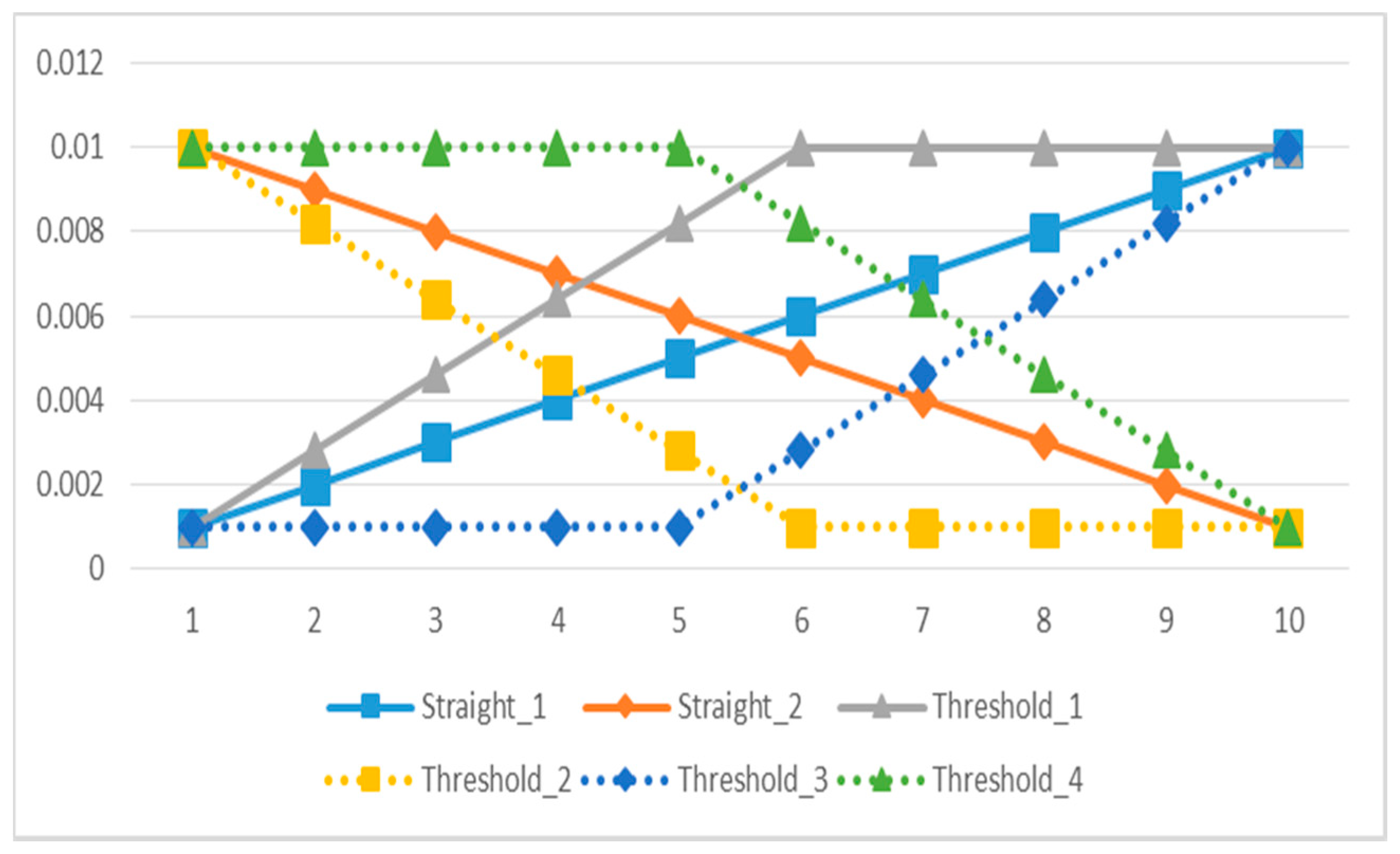
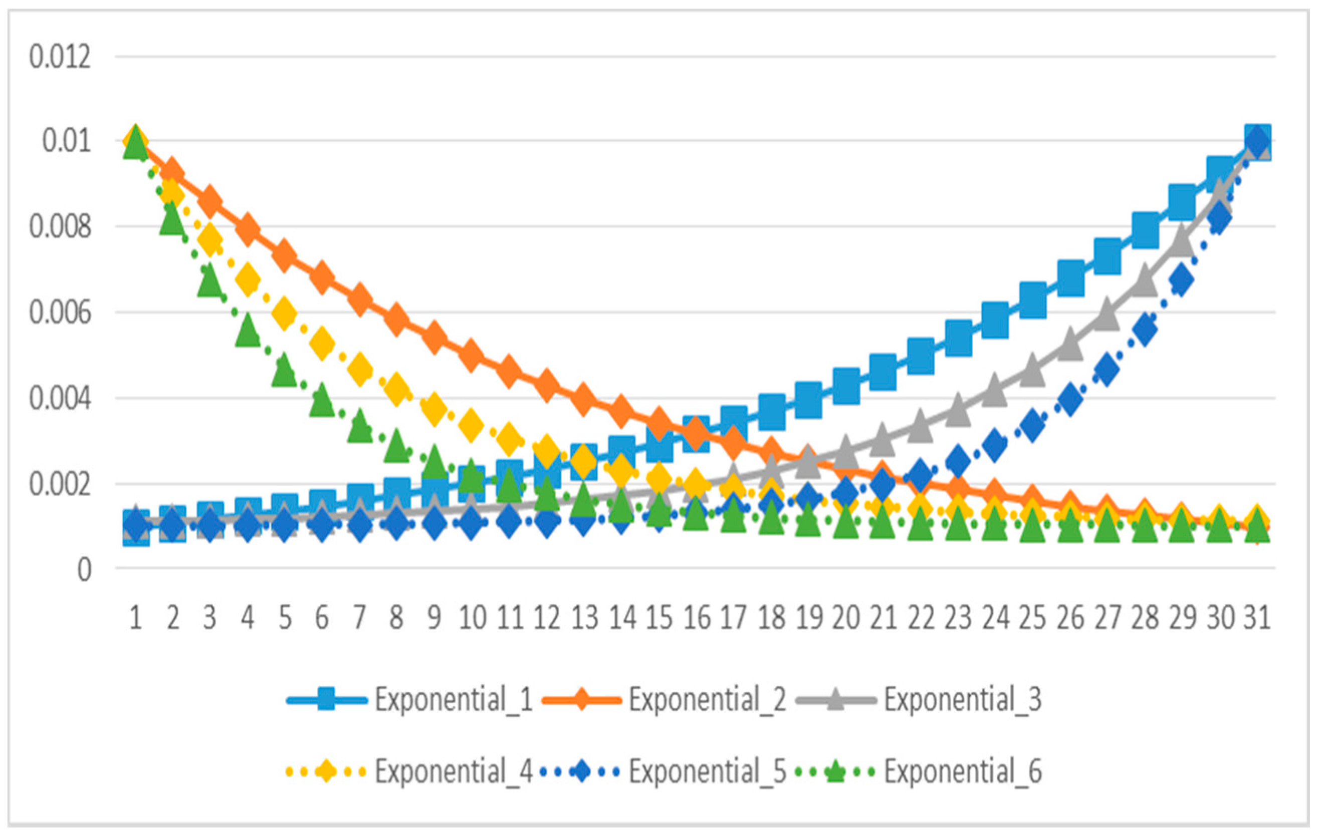
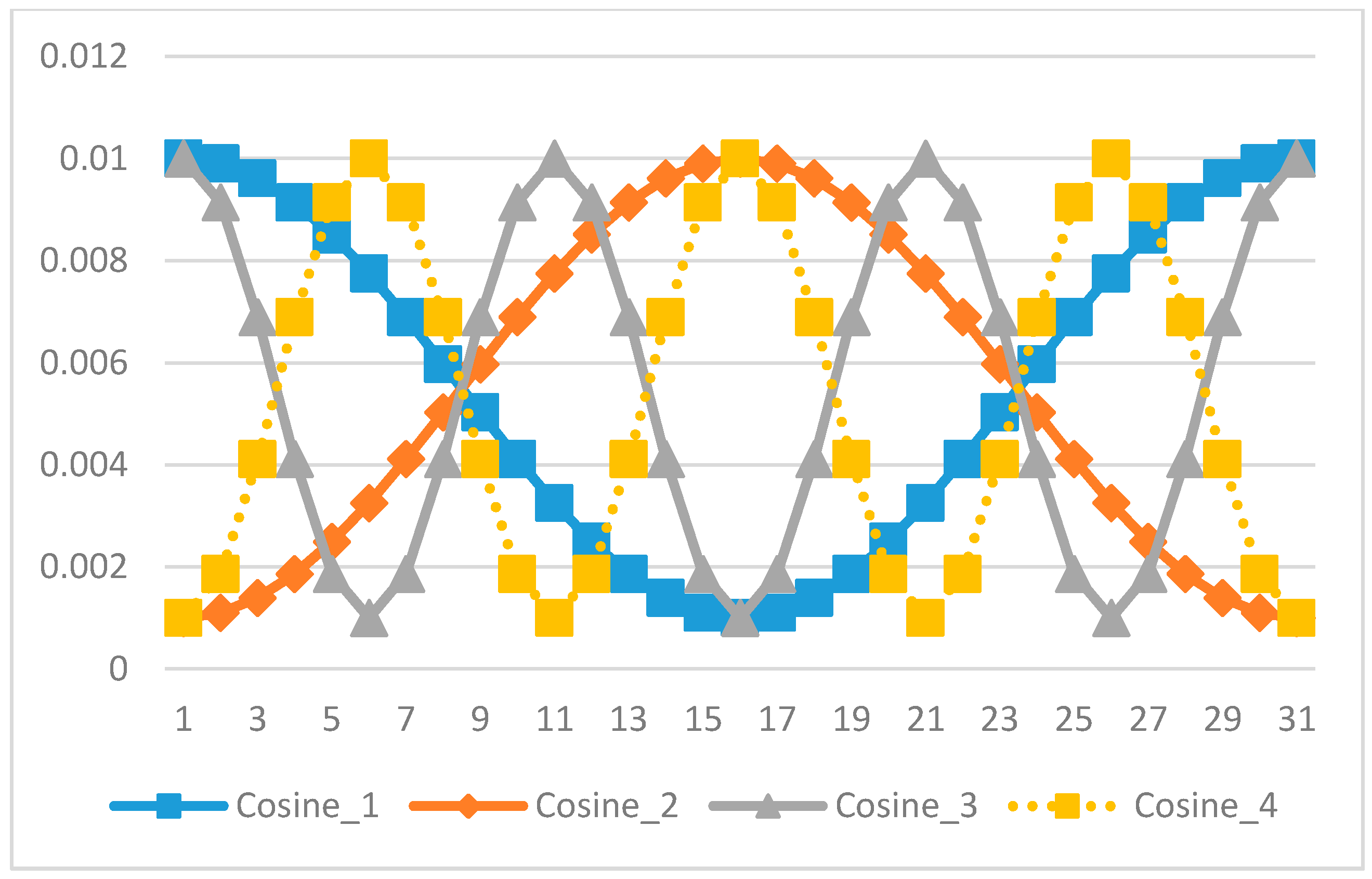
Appropriate parameters can enhance the searching ability of a metaheuristic algorithm. Inspired by this concept, a dynamic adjusting NGHS (DANGHS) is presented in this section. In the DANGHS, the genetic mutation probability ( p m ) is dynamically adjusted in each iteration. However, we can enhance the searching ability of the NGHS algorithm by many kinds of dynamic adjustment strategies. Therefore, we introduced 16 dynamic adjustment strategies in this paper. All 16 strategies are shown as follows, and Figure 4, Figure 5 and Figure 6 are used to illustrate the 16 strategies.
(1)
Straight linear increasing strategy (Straight_1):
The genetic mutation probability is increased by Equation (6), which is a linear function.
p m k = p m _ m i n + ( p m _ m a x p m _ m i n ) N I × k .
Here, p m _ m i n is the minimum genetic mutation probability, and p m _ m a x is the maximum genetic mutation probability.
(2)
Straight linear decreasing strategy (Straight_2):
The genetic mutation probability is decreased by Equation (7), which is a linear function.
p m k = p m _ m a x + ( p m _ m i n p m _ m a x ) N I × k
(3)
Threshold linear prior increasing strategy (Threshold_1):
The genetic mutation probability is increased by Equation (8), which is a linear function with a threshold. The genetic mutation probability is raised before the threshold, but the genetic mutation probability is a fixed maximum value after the threshold.
p m k = { p m _ m i n + P m _ m a x P m _ m i n N I × 2 k i f   k < N I / 2 p m _ m a x i f   k N I / 2
(4)
Threshold linear prior decreasing strategy (Threshold_2):
The genetic mutation probability is decreased by Equation (9), which is a linear function with a threshold. The genetic mutation probability is reduced before the threshold, but the genetic mutation probability is a fixed minimum value after the threshold.
p m k = { p m _ m a x + P m _ m i n P m _ m a x N I × 2 k i f   k < N I / 2 p m _ m i n i f   k N I / 2
(5)
Threshold linear posterior increasing strategy (Threshold_3):
The genetic mutation probability is increased by Equation (10), which is a linear function with a threshold. The genetic mutation probability is a fixed minimum value before the threshold, but the genetic mutation probability is raised after the threshold.
p m k = { p m _ m i n i f   k < N I / 2 p m _ m i n + P m _ m a x P m _ m i n N I × 2 k i f   k N I / 2
(6)
Threshold linear posterior decreasing strategy (Threshold_4):
The genetic mutation probability is decreased by Equation (11), which is a linear function with a threshold. The genetic mutation probability is a fixed maximum value before the threshold, but the genetic mutation probability is reduced after the threshold.
p m k = { p m _ m a x i f   k < N I / 2 p m _ m a x + P m _ m i n P m _ m a x N I × 2 k i f   k N I / 2
(7)
Natural exponential increasing strategy (Exponential_1):
The genetic mutation probability is increased by Equation (12), which is a non-linear function.
p m k = p m _ m i n × e ( ln ( p m _ m a x p m _ m i n ) × k / N I )
(8)
Natural exponential decreasing strategy (Exponential_2):
The genetic mutation probability is decreased by Equation (13), which is a non-linear function.
p m k = p m _ m a x × e ( ln ( p m _ m i n p m _ m a x ) × k / N I )
(9)
Exponential increasing strategy:
The genetic mutation probability is increased by Equation (14), which is a non-linear function. We can control the increasing rate by the modification rate ( m r ).
p m k = p m _ m i n + ( p m _ m a x p m _ m i n ) × m r ( N I k ) / N I
In this paper, the m r is equal to 0.01 or 0.001. Therefore, in this paper, the 9th strategy (Exponential_3) is the exponential increasing strategy with m r = 0.01 , and the 10th strategy (Exponential_5) is the exponential increasing strategy with m r = 0.001 .
(10)
Exponential decreasing strategy:
The genetic mutation probability is decreased by Equation (15), which is a non-linear function. We can control the decreasing rate by the modification rate ( m r ).
p m k = p m _ m i n + ( p m _ m a x p m _ m i n ) × m r k / N I
In this paper, the m r is equal to 0.01 or 0.001. Therefore, in this paper, the 11th strategy (Exponential_4) is the exponential decreasing strategy with m r = 0.01 , and the 12th strategy (Exponential_6) is the exponential decreasing strategy with m r = 0.001 .
(11)
Concave cosine strategy:
The genetic mutation probability is changed by Equation (16), which is a periodic function. The shape of this function is a concave, and we can control the cycle time of this function by the coefficient of cycle (cc).
p m k = p m _ m a x + p m _ m i n 2 + p m _ m a x p m _ m i n 2 × cos k × c c × 2 π N I
In this paper, the c c is equal to 1 or 3. Therefore, in this paper, the 13th strategy (Cosine_1) is the concave cosine strategy with c c = 1 , and the 14th strategy (Cosine_3) is the concave cosine strategy with c c = 3 .
(12)
Convex cosine strategy:
The genetic mutation probability is changed by Equation (17), which is a periodic function. The shape of this function is a convex, and we can control the cycle time of this function by the coefficient of cycle (cc).
p m k = p m _ m a x + p m _ m i n 2 p m _ m a x p m _ m i n 2 × cos k × c c × 2 π N I
In this paper, the c c is equal to 1 or 3. Therefore, in this paper, the 15th strategy (Cosine_2) is the convex cosine strategy with c c = 1 , and the 16th strategy (Cosine_4) is the convex cosine strategy with c c = 3 .
In general, the DANGHS algorithm works as follows:
Step 1. Initialization: the problem and algorithm parameters
The parameters are the harmony memory size (m), the current iteration k = 1, and the maximum number of iterations (NI).
Step 2. Initialization: the decision variable values and the harmony memory
The initial decision variable values x i j k = 0 ( i = 1 ,   2 ,   ,   m ) is generated by Equation (1). The HM is as shown in Equation (2).
Step 3. Movement: generate the algorithm parameters
Generate the genetic mutation probability ( p m k ) in each iteration by dynamic adjustment strategies.
Step 4. Movement: improvise a new harmony
The DANGHS movement step (Pseudocode 4) is shown in Algorithm 4.
Algorithm 4 The Movement Steps of DANGHS (Pseudocode 4)
1:For j = 1   to   D do
2:  If r 1 > p m k then
3:    x R = 2 × x best , j k x worst , j k
4:   If x R > x jU then
5:     x R = x jU
6:   Else if x R < x jL then
7:     x R = x jL
8:   End
9:    x j k + 1 = x worst , j k + r 2 × ( x R x worst , j k )  % position updating
10:  Else
11:    x j k + 1 = x jL + r 3 × ( x jU x jL )  % genetic mutation
12:  End
13:End
Here, x b e s t , j k and x w o r s t , j k are the best harmony and the worst harmony in the HM, respectively. r 1 , r 2 and r 3 are uniformly generated random numbers in [0, 1]. r 1 determines whether DANGHS should carry out genetic mutation, r 2 is used for position updating, and r 3 is used for genetic mutation.
Step 5. Replacement: update harmony memory
DANGHS replaces the worst harmony x w o r s t , j k ( j = 1 ,   2 ,   ,   D ) in the HM by the new harmony x k + 1 , even if the new harmony is worse than the worst harmony.
Step 6. Iteration: check the stopping criterion
If the stopping criterion (maximum number of iterations NI) is satisfied, terminate the computation and return the best harmony vector x b e s t in the HM; otherwise, the current iteration k = k + 1 and go back to step 3.

4. Experiments and Analysis

In order to verify the performance of the 16 dynamic adjustment strategies in the DANGHS algorithm, 14 well-known benchmark optimization problems [24,28,31] are considered, as shown in Table 1. This study used Python 3.6.2 (64-bit) as the complier to write the program for finding the solution. The solution-finding equipment was an Intel Core (TM) i7-4720HQ (2.6 GHz) CPU, 8G of memory, and Windows 10 home edition (64-bit) OS.
Problems 1–4, 10 and 11, which are Sphere function, Step function, Schwefel’s problem 2.22, Rotated hyper-ellipsoid function, Shifted Sphere function, and Shifted Rotated hyper-ellipsoid function, are unimodal problems. Problems 5–9 and 12–14, which are Griewank function, Ackley’s function, Rosenbrock function, Rastrigin function, Schwefel’s problem 2.26, Shifted Rotated Griewank function, Shifted Rosenbrock function, and Shifted Rastrigin function, are difficult multimodal problems; i.e., there are several local optima in these problems and the number of local optima increases with the problem dimension (D) [24].
In order to verify the performance of the DANGHS algorithm, this paper compared the extensive experiment results of the DANGHS algorithm with other different HS algorithms. In the experiments, the parameters of the compared HS algorithms are shown in Table 2 [28].
In all HS algorithms, the harmony memory size (m) is 5. For each problem, two different dimension sizes (D) are tested, and they are equal to 30 and 100. Therefore, the iteration number are equal to 60,000 and 150,000, respectively. Thirty independent experiments (n) are carried out for each problem. The experimental results obtained using the 16 proposed adjustment strategies in the DANGHS algorithms and those obtained using different HS algorithms are shown in Table 3 and Table 4, respectively. In the two tables, SD represents the standard deviation.
In Table 3, several experimental results are given. First of all, the best results given by the same strategy for different dimension sizes are obtained for problems 1, 3, 6, 9 and 13. Among these problems, the decreasing strategy can find the best objective function value for problems 1, 3, 6, and 9. According to the experimental results, the exponential decreasing strategy with mr = 0.001 (Exponential_6) can find the best objective function value for problems 1 (1.8344 × 10⁻³¹; 1.2209 × 10⁻¹⁴), 3 (1.9511 × 10⁻¹⁸ 7.9778 × 10⁻⁹) and 6 (9.6308 × 10⁻¹⁴; 9.3030 × 10⁻⁹); the threshold linear prior decreasing strategy (Threshold_2) can find the best objective function value for problem 9 (3.8183 × 10⁻⁴; 1.2728 × 10⁻³). More specifically, the convex cosine strategy with k = 3 (Cosine_4), which is the periodic strategy, can find the best objective function value for problem 13 (3.9875 × 10²; 5.3644 × 10²).
On the other hand, the best results given by different strategies for different dimension sizes are obtained for problems 4, 5, 7, 8, 10, 11, 12, and 14. Among these problems, the increasing strategy can find the best objective function value for problem 7. According to the experimental results, the straight linear increasing strategy (Straight_1) can find the best objective function value for problem 7 with D = 30 (1.0089 × 101). However, the threshold linear posterior increasing strategy (Threshold_3) can find the best objective function value for problem 7 with D = 100 (6.1559 × 101). Besides, the decreasing strategy can find the best objective function value for problems 4, 5, 10, 11, 12, and 14. According to the experimental results, the threshold linear posterior decreasing strategy (Threshold_4) can find the best objective function value for problems 4 (6.0249 × 101), 5 (3.1209 × 10⁻²) and 11 (−3.7419 × 10²) with D = 30. However, the natural exponential decreasing strategy (Exponential_2) can find the best objective function value for problems 4 (8.6301 × 10³), 5 (6.4754 × 10⁻³), and 11 (1.1471 × 10⁴) with D = 100. The natural exponential decreasing strategy (Exponential _2) can find the best objective function value for problem 10 with D = 30 (−4.5000 × 10²). However, the threshold linear prior decreasing strategy (Threshold_2) can find the best objective function value for problem 10 with D = 100 (−4.5000 × 10²). The straight linear decreasing strategy (Straight_2) can find the best objective function value for problem 12 with D = 30 (−1.7821 × 10²). However, the exponential decreasing strategy with m r = 0.001 (Exponential_6) can find the best objective function value for problem 12 with D = 100 (−1.6037 × 10²). The straight linear decreasing strategy (Straight_2) can find the best objective function value for problem 14 with D = 30 (−3.3000 × 10²). However, the exponential decreasing strategy with m r = 0.01 (Exponential_4) can find the best objective function value for problem 14 with D = 100 (−3.2997 × 10²).
Particularly, for problem 8, the decreasing strategy can find the best objective function value when D = 30, however the increasing strategy can find the best objective function value when D = 100. In other words, the threshold linear prior decreasing strategy (Threshold_2) can find the best objective function value for problem 8 with D = 30 (0.0000). However, the exponential increasing strategy with m r = 0.01 (Exponential_3) can find the best objective function value for problem 8 with D = 100 (2.7729 × 10⁻²).
In Table 3, the best results are presented by the boldface type. For example, the Threshold_2 strategy had the best minimum objective function value for problems 1 with D = 30 (7.1381 × 10−39). The Exponential_6 strategy had the best maximum objective function value (3.7601 × 10⁻³⁰) and had the minimum standard deviation value (7.0604 × 10⁻³¹) for problems 1 with D = 30.
In Table 4, among all problems for D = 30, the DANGHS algorithm can find the best objective function value for problems 1–3, 6–10, and 14. The SGHS algorithm can find the best objective function value for problems 2, 4, and 11. The NGHS algorithm can find the best objective function value for problems 2, 12, and 13. The IHS algorithm can find the best objective function value for problem 5. The best algorithms and the best results are presented by the boldface type in Table 4.
On the other hand, among all problems for D = 100, the DANGHS algorithm can find the best objective function value for problems 1–14. The NGHS algorithm can find the best objective function value for problem 2.
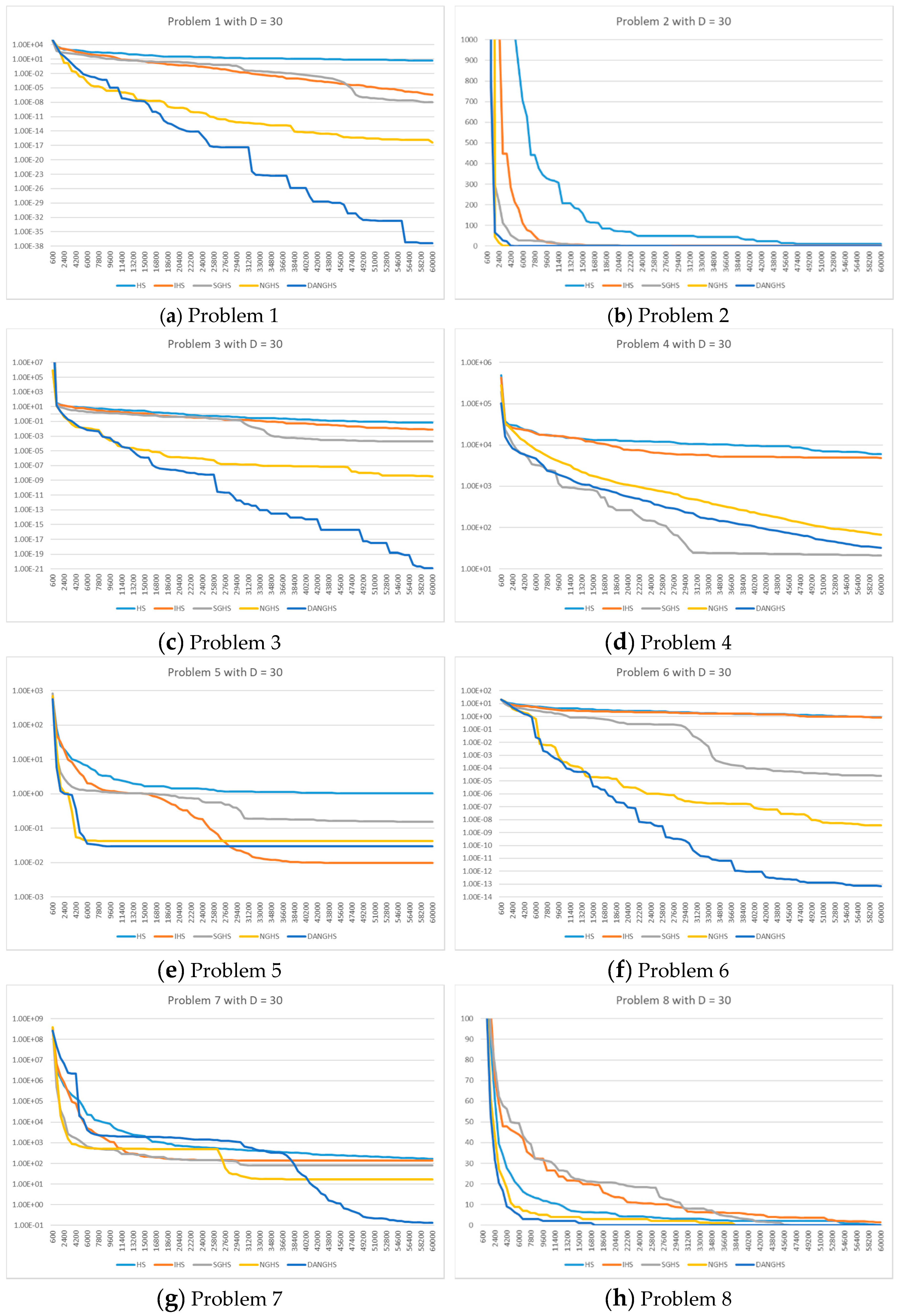
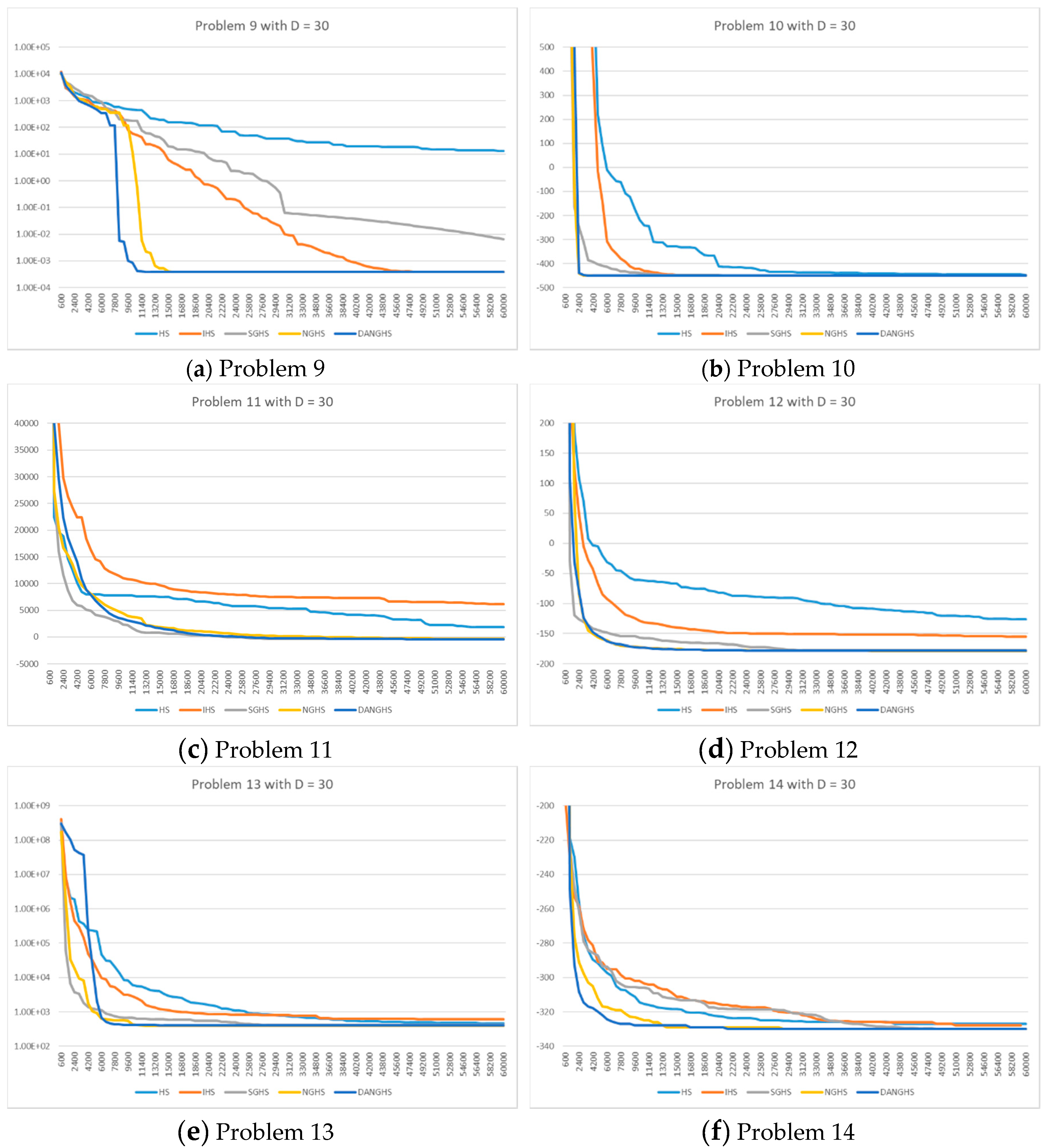
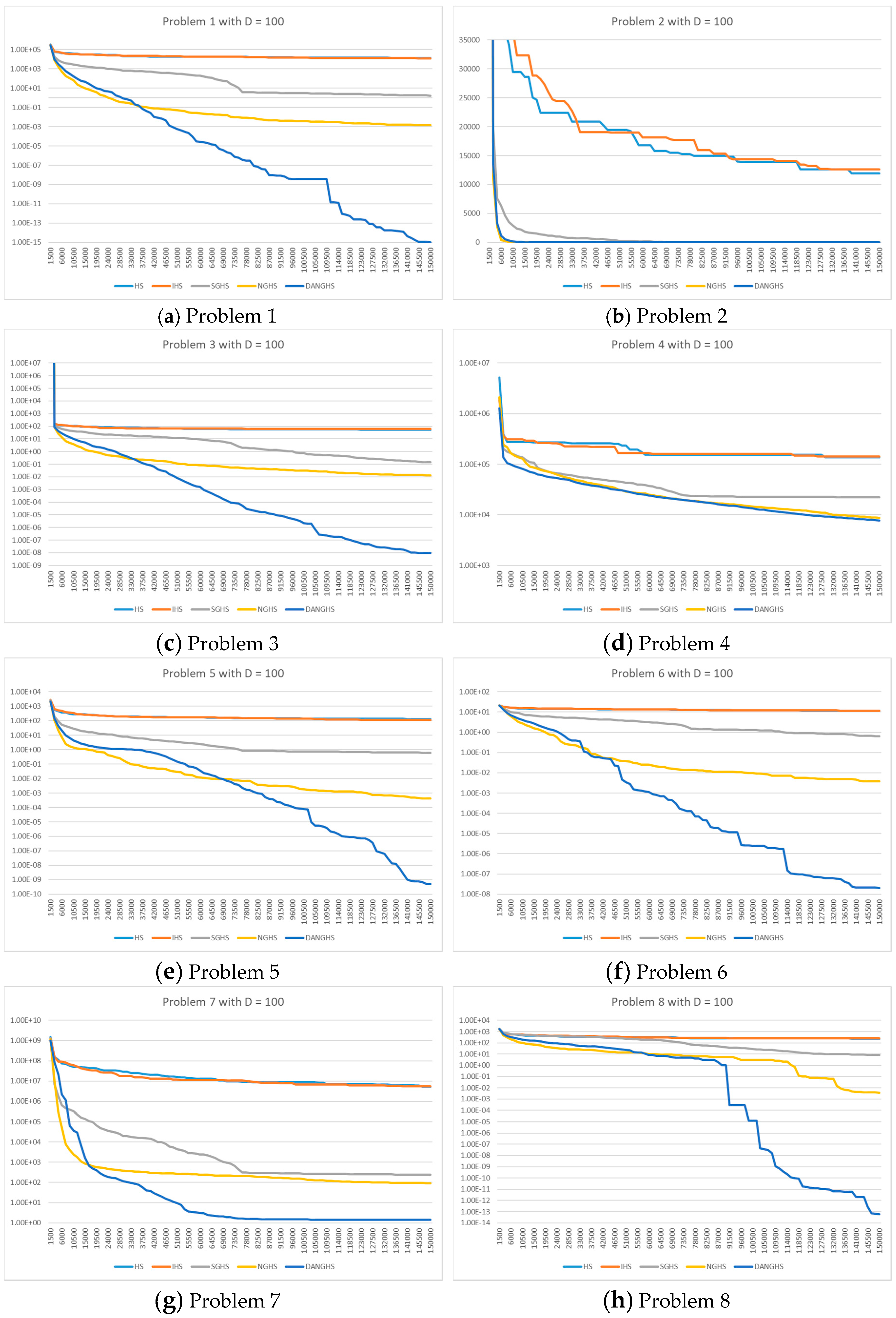
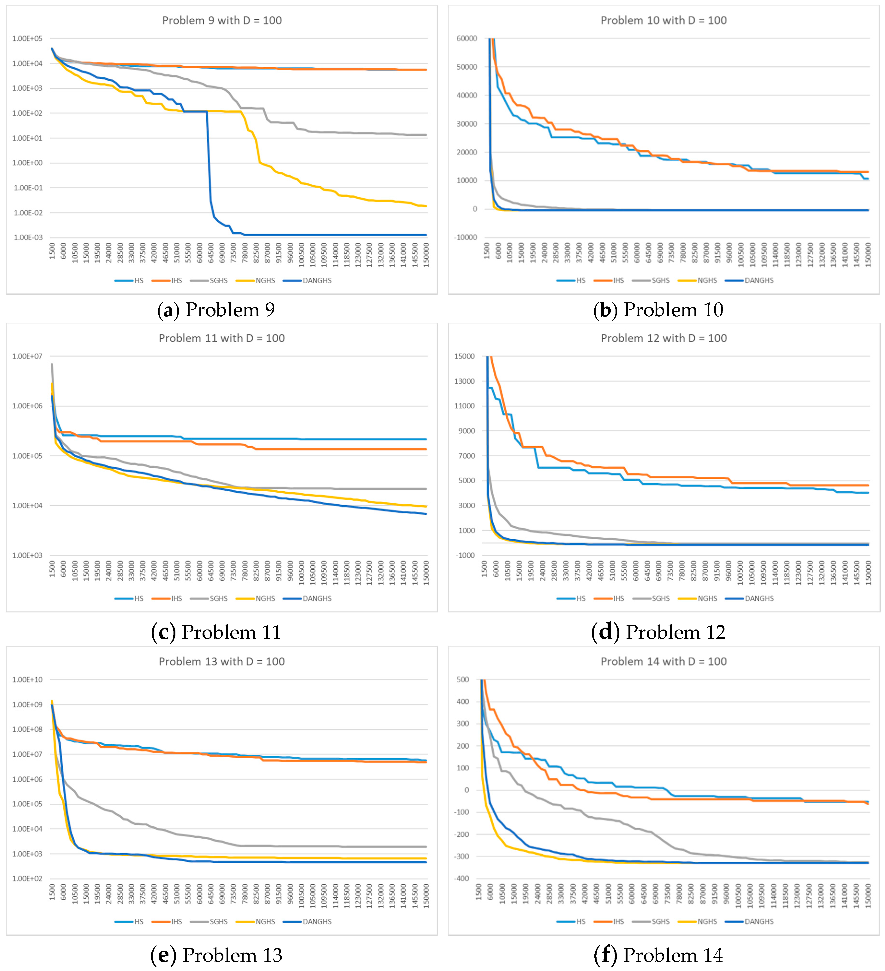
Figure 7 presents a typical solution history graph of five different algorithms along iterations for problems 1 to 8 with D = 30, and Figure 8 presents a typical solution history graph of five different algorithms along iterations for problems 9 to 14 with D = 30. Figure 9 presents a typical solution history graph of five different algorithms along iterations for problems 1 to 8 with D = 100, and Figure 10 presents a typical solution history graph of five different algorithms along iterations for problems 9 to 14 with D = 100.
Finally, we will discuss and analyze the efficiency of the DANGHS algorithm. In Figure 7, Figure 8, Figure 9 and Figure 10, we can easily find out that the DANGHS algorithm obviously had the better searching performance and convergence ability than other algorithms in most low-dimensional problems and in all high-dimensional problems. In other words, the DANGHS algorithm can use the less iterations to solve the problem and is more efficient than other HS algorithms. Besides, according to the experimental results, the DANGHS with Pseudocode 3 spent 603.5025 seconds to run 30 experiments; while the DANGHS with Pseudocode 4 spent 532.7705 seconds only to run 30 experiments. The DANGHS algorithm with Pseudocode 4 reduces 11.72% of the running time, as compared with Pseudocode 3. Therefore, the DANGHS algorithm with the proposed Pseudocode 4 is more efficient than with Pseudocode 3.

5. Conclusions

We presented a DANGHS algorithm, which combines NGHS and the dynamic adjustment strategy for genetic mutation probability. Moreover, the extensive computational experiments and comparisons were carried out for 14 benchmark continuous optimization problems. According to the extensive computational results, there are several findings in this paper worth summarizing.
First, different strategies are suitable for different problems.
  • The decreasing dynamic adjustment strategies should be applied to some problems in which the DANGHS algorithm needs a larger, p m , in the early iterations, in order to have a larger probability of finding a better trial solution around the current one.
  • The increasing dynamic adjustment strategies should be applied to other problems. For these problems, if the current solution is trapped in a local optimum, the DANGHS algorithm requires a larger probability, p m , in later iterations in order to avoid the local optima.
  • The periodic dynamic adjustment strategy can find the best objective function value for problem 13. These particular results show that there are not only two kinds of adjustment strategies, decreasing and increasing strategies, which are suitable for all problems. This viewpoint is different from the common views: the adjustment strategy is as small as possible or as large as possible with a generation number. For a specific problem, the periodic dynamic adjustment strategy could have better performance in comparison with other decreasing or increasing strategies. Therefore, these results inspire us to further investigate this kind of periodic dynamic adjustment strategy in future experiments.
Second, the extensive experimental results showed that the DANGHS algorithm had better searching performance in comparison with other HS algorithms for D = 30 and 100 in most problems. Particularly for D = 100, the DANGHS algorithm could search the best objective function value in all 14 problems. In other words, the DANGHS had superior searching performance in high-dimensional problems. According to the numerical results, we proofed that algorithms with dynamic parameters, such as the DANGHS algorithm and the IHS algorithm, could have better searching performance than algorithms without dynamic parameters, such as the NGHS algorithm and the HS algorithm. Moreover, according to these results, we proofed that the viewpoint presented in previous studies is suitable for the NGHS algorithm. This viewpoint states that appropriate parameters can enhance the searching ability of a metaheuristic algorithm.
Finally, the DANGHS algorithm using Pseudocode 4 was more efficient than that using Pseudocode 3. In Pseudocode 3, the algorithm generates a new harmony, and then with p m probability, the algorithm abandoned it to generate a mutated harmony. Obviously, it was redundant and inefficient. Therefore, we modified the procedure in Pseudocode 3 and presented a more efficient Pseudocode 4 in this paper. In conclusion, the DANGHS algorithm is a more efficient and effective algorithm.
Author Contributions

P.-C.S. designed the algorithm, conducted the experiments, analyzed the experimental results, wrote the paper and polished the English; C.-Y.C. and X.L. supervised the research work and provided helpful suggestions.

Funding

This research received no external funding.

Acknowledgments

The authors would like to thank all the reviewers for their constructive comments.

Conflicts of Interest

The authors declare no conflict of interest.

References

  1. Chiu, C.Y.; Fan, S.K.S.; Shih, P.C.; Weng, Y.H. Applying HBMO-based SOM in predicting the Taiwan steel price fluctuation. Int. J. Electron. Bus. Manag. 2014, 12, 1–14. [Google Scholar]
  2. Chen, K.H.; Chen, L.F.; Su, C.T. A new particle swarm feature selection method for classification. J. Intell. Inf. Syst. 2014, 42, 507–530. [Google Scholar] [CrossRef]
  3. Petrović, M.; Vuković, N.; Mitić, M.; Miljković, Z. Integration of process planning and scheduling using chaotic particle swarm optimization algorithm. Expert Syst. Appl. 2016, 64, 569–588. [Google Scholar] [CrossRef]
  4. Khaled, N.; Hemayed, E.E.; Fayek, M.B. A GA-based approach for epipolar geometry estimation. Int. J. Pattern Recognit. Artif. Intell. 2013, 27, 1355014. [Google Scholar] [CrossRef]
  5. Metawaa, N.; Hassana, M.K.; Elhoseny, M. Genetic algorithm based model for optimizing bank lending decisions. Expert Syst. Appl. 2017, 80, 75–82. [Google Scholar] [CrossRef]
  6. Song, S. Design of distributed database systems: an iterative genetic algorithm. J. Intell. Inf. Syst. 2015, 45, 29–59. [Google Scholar] [CrossRef]
  7. Gambardella, L.M.; Montemanni, R.; Weyland, D. Coupling ant colony systems with strong local searches. Eur. J. Oper. Res. 2012, 220, 831–843. [Google Scholar] [CrossRef]
  8. D’Andreagiovanni, F.; Mett, F.; Nardin, A.; Pulaj, J. Integrating LP-guided variable fixing with MIP heuristics in the robust design of hybrid wired-wireless FTTx access networks. Appl. Soft. Comput. 2017, 61, 1074–1087. [Google Scholar] [CrossRef]
  9. D’Andreagiovanni, F.; Nardin, A. Towards the fast and robust optimal design of wireless body area networks. Appl. Soft. Comput. 2015, 37, 971–982. [Google Scholar] [CrossRef] [Green Version]
  10. Kennedy, J.; Eberhart, R. Particle Swarm Optimization. In Proceedings of the IEEE International Conference on Neural Networks, Perth, Australia, 27 November–1 December 1995. [Google Scholar]
  11. Eberhart, R.; Kennedy, J. A new optimizer using particle swarm theory. In Proceedings of the Sixth International Symposium on Micro Machine and Human Science, Nagoya, Japan, 4–6 October 1995; pp. 39–43. [Google Scholar]
  12. Ozcan, E.; Mohan, C.K. Analysis of a simple particle swarm optimization system. Intell. Eng. Syst. Artif. Neural Netw. 1998, 8, 253–258. [Google Scholar]
  13. Holland, J.H. Adaptation in Natural and Artificial Systems: An Introductory Analysis with Applications to Biology, Control and Artificial Intelligence; University of Michigan Press: Ann Arbor, MI, USA, 1975. [Google Scholar]
  14. Holland, J.H. Adaptation in Natural and Artificial Systems: An Introductory Analysis with Applications to Biology, Control, and Artificial Intelligence; MIT Press: Cambridge, MA, USA, 1992. [Google Scholar]
  15. Gordini, N. A genetic algorithm approach for SMEs bankruptcy prediction: Empirical evidence from Italy. Expert Syst. Appl. 2014, 41, 6433–6445. [Google Scholar] [CrossRef]
  16. Geem, Z.W.; Kim, J.H.; Loganathan, G.V. A new heuristic optimization algorithm: harmony search. Simulation 2001, 76, 60–68. [Google Scholar] [CrossRef]
  17. Haddad, O.B.; Afshar, A.; Marino, M.A. Honey-bees mating optimization (HBMO) algorithm: A new heuristic approach for water resources optimization. Water Resour. Manag. 2006, 20, 661–680. [Google Scholar] [CrossRef]
  18. Ouyang, A.; Peng, X.; Liu, Y.; Fan, L.; Li, K. An efficient hybrid algorithm based on HS and SFLA. Int. J. Pattern Recognit. Artif. Intell. 2016, 30, 1659012. [Google Scholar] [CrossRef]
  19. Tavakoli, S.; Valian, E.; Mohanna, S. Feedforward neural network training using intelligent global harmony search. Evol. Syst. 2012, 3, 125–131. [Google Scholar] [CrossRef]
  20. Kirkpatrick, S.; Gelatt, C.D.; Vecchi, M.P. Optimization by simulated annealing. Science 1983, 220, 671–680. [Google Scholar] [CrossRef] [PubMed]
  21. Assad, A.; Deep, K. A Hybrid Harmony search and Simulated Annealing algorithm for continuous optimization. Inf. Sci. 2018, 450, 246–266. [Google Scholar] [CrossRef]
  22. Assad, A.; Deep, K. A two-phase harmony search algorithm for continuous optimization. Comput. Intell. 2017, 33, 1038–1075. [Google Scholar] [CrossRef]
  23. Mahdavi, M.; Fesanghary, M.; Damangir, E. An improved harmony search algorithm for solving optimization problems. Appl. Math. Comput. 2007, 188, 1567–1579. [Google Scholar] [CrossRef]
  24. Pan, Q.K.; Suganthan, P.N.; Tasgetiren, M.F.; Liang, J.J. A self-adaptive global best harmony search algorithm for continuous optimization problems. Appl. Math. Comput. 2010, 216, 830–848. [Google Scholar] [CrossRef]
  25. Zou, D.; Gao, L.; Li, S.; Wu, J.; Wang, X. A novel global harmony search algorithm for task assignment problem. J. Syst. Softw. 2010, 83, 1678–1688. [Google Scholar] [CrossRef]
  26. Zou, D.; Gao, L.; Wu, J.; Li, S.; Li, Y. A novel global harmony search algorithm for reliability problems. Comput. Ind. Eng. 2010, 58, 307–316. [Google Scholar] [CrossRef]
  27. Zou, D.; Gao, L.; Wu, J.; Li, S. Novel global harmony search algorithm for unconstrained problems. Neurocomputing 2010, 73, 3308–3318. [Google Scholar] [CrossRef]
  28. Valian, E.; Tavakoli, S.; Mohanna, S. An intelligent global harmony search approach to continuous optimization problems. Appl. Math. Comput. 2014, 232, 670–684. [Google Scholar] [CrossRef]
  29. Kattan, A.; Abdullah, R. Training of feed-forward neural networks for pattern-classification applications using music inspired algorithm. Inter. J. Comput. Sci. Inf. Secur. 2011, 9, 44–57. [Google Scholar]
  30. Lee, K.S.; Geem, Z.W. A new meta-heuristic algorithm for continuous engineering optimization: harmony search theory and practice. Comput. Method Appl. Mech. Eng. 2005, 194, 3902–3933. [Google Scholar] [CrossRef]
  31. Omran, M.G.H.; Mahdavi, M. Global-best harmony search. Appl. Math. Comput. 2008, 198, 643–656. [Google Scholar] [CrossRef]
Figure 1. (a) Variation of pitch adjusting rate (PAR) versus iteration number; (b) Variation of bandwidth (BW) versus iteration number.
Symmetry 10 00337 g001
Figure 2. Comparison between music improvisation and engineering optimization.
Symmetry 10 00337 g002
Figure 3. Schematic diagram of position updating.
Symmetry 10 00337 g003
Figure 4. Straight linear and threshold linear strategies.
Symmetry 10 00337 g004
Figure 5. Exponential strategies.
Symmetry 10 00337 g005
Figure 6. Concave cosine and convex cosine strategies.
Symmetry 10 00337 g006
Figure 7. Typical convergence graph of five different algorithms for problems 1 to 8 (D = 30). (a) Problem 1; (b) Problem 2; (c) Problem 3; (d) Problem 4; (e) Problem 5; (f) Problem 6; (g) Problem 7; (h) Problem 8.
Symmetry 10 00337 g007
Figure 8. Typical convergence graph of five different algorithms for problems 9 to 14 (D = 30). (a) Problem 9; (b) Problem 10; (c) Problem 11; (d) Problem 12; (e) Problem 13; (f) Problem 14.
Symmetry 10 00337 g008
Figure 9. Typical convergence graph of five different algorithms for problems 1 to 8 (D = 100). (a) Problem 1; (b) Problem 2; (c) Problem 3; (d) Problem 4; (e) Problem 5; (f) Problem 6; (g) Problem 7; (h) Problem 8.
Symmetry 10 00337 g009
Figure 10. Typical convergence graph of five different algorithms for problems 9 to 14 (D = 100). (a) Problem 9; (b) Problem 10; (c) Problem 11; (d) Problem 12; (e) Problem 13; (f) Problem 14.
Symmetry 10 00337 g010
Table 1. 14 well-known benchmark optimization problems.
NameFunctionSearch SpaceOptimum
f 1 Sphere function min f ( x i ) = i = 1 N x i 2 [−100, 100]n0
f 2 Step function min f ( x i ) = i = 1 N ( x i + 0.5 ) 2 [−100, 100]n0
f 3 Schwefel’s problem 2.22 min f ( x i ) = i = 1 N | x i | + i = 1 N | x i | [−10, 10]n0
f 4 Rotated hyper-ellipsoid function min f ( x i ) = i = 1 N ( j = 1 i x j ) 2 [−100, 100]n0
f 5 Griewank function min f ( x i ) = 1 4000 i = 1 N x i 2 i = 1 N cos ( x i i ) + 1 [−600, 600]n0
f 6 Ackley’s function min f ( x i ) = 20 + e 20 exp ( 0.2 i = 1 N x i 2 / n ) exp ( i = 1 N cos ( 2 π x i ) / n ) [−32, 32]n0
f 7 Rosenbrock function min f ( x i ) = i = 1 N 1 ( 100 ( x i + 1 x i 2 ) 2 + ( 1 x i ) 2 ) [−30, 30]n0
f 8 Rastrigin function min f ( x i ) = i = 1 N ( x i 2 10 cos ( 2 π x i ) + 10 ) [−5.12, 5.12]n0
f 9 Schwefel’s problem 2.26 min f ( x i ) = 418.9829 N i = 1 N ( x i sin ( | x i | ) ) [−500, 500]n0
f 10 Shifted Sphere function min f ( x i ) = i = 1 N z i 2 450 [−100, 100]n−450
f 11 Shifted Rotated hyper-ellipsoid function min f ( x i ) = i = 1 N ( j = 1 i z i ) 2 450 [−100, 100]n−450
f 12 Shifted Rotated Griewank function min f ( x i ) = 1 4000 i = 1 N z i 2 i = 1 N cos ( z i i ) + 1 180 [−600, 600]n−180
f 13 Shifted Rosenbrock function min f ( x i ) = i = 1 N 1 ( 100 ( z i + 1 z i 2 ) 2 + ( 1 z i ) 2 ) + 390 [−30, 30]n390
f 14 Shifted Rastrigin function min f ( x i ) = i = 1 N ( z i 2 10 cos ( 2 π z i ) + 10 ) 330 [−5.12, 5.12]n−330
Table 2. Parameters of compared harmony search (HS) algorithms.
Algorithmm 1HMCR 2PAR 3BW 4LP 5 p m 6
HS50.90.30.01
IHS50.9 P A R m i n = 0.01
P A R m a x = 0.99
B W m a x = ( x j U x j L ) / 20
B W m i n = 0.0001
SGHS5 H M C R m = 0.98 P A R m = 0.9 B W m a x = ( x j U x j L ) / 10
B W m i n = 0.0005
100
NGHS50.005
DANGHS5 P m i n = 0.001
P m a x = 0.010 .
1 m: the harmony memory size; 2 HMCR: the harmony memory considering rate; 3 PAR: the pitch adjusting rate; 4 BW: the bandwidth; 5 LP: the learning period; 6 p m : the genetic mutation probability.
Table 3. Experimental results of 16 strategies in the DANGHS algorithms.
No.Dimension (D) = 30Dimension (D) = 100
Adjustment strategyMinMaxMeanSDAdjustment strategyMinMaxMeanSD
f 1 Straight_11.0461 × 10−174.3759 × 10−156.7177 × 10−161.1026 × 10⁻¹⁵Straight_17.4075 × 10−63.1563 × 10−43.3196 × 10−55.3403 × 10⁻⁵
Straight_23.1999 × 10−232.5783 × 10−183.6341 × 10−196.7121 × 10⁻¹⁹Straight_21.0715 × 10−77.1045 × 10−68.4864 × 10−71.2362 × 10⁻⁶
Threshold_11.5431 × 10−137.3069 × 10−116.6315 × 10−121.3094 × 10⁻¹¹Threshold_11.0024 × 10−39.1452 × 10−32.7025 × 10−31.6455 × 10⁻³
Threshold_27.1381 × 10−392.0446 × 10−266.8264 × 10−283.6700 × 10⁻²⁷Threshold_23.9739 × 10−168.5814 × 10−141.7158 × 10−142.2275 × 10⁻¹⁴
Threshold_31.5233 × 10−321.4639 × 10−224.9489 × 10−242.6266 × 10⁻²³Threshold_35.5110 × 10−154.3556 × 10−123.2639 × 10−137.8921 × 10⁻¹³
Threshold_43.3374 × 10−184.3038 × 10−121.4919 × 10−137.7155 × 10⁻¹³Threshold_43.2962 × 10−51.8976 × 10−48.5947 × 10−54.0524 × 10⁻⁵
Exponential_11.5745 × 10−241.0309 × 10−184.3948 × 10−201.8663 × 10⁻¹⁹Exponential_12.6917 × 10−94.3964 × 10−81.3508 × 10−89.5937 × 10⁻⁹
Exponential_21.9177 × 10−309.0711 × 10−234.0772 × 10−241.6377 × 10⁻²³Exponential_23.3307 × 10−112.2886E × 10−94.9657 × 10−105.7327 × 10⁻¹⁰
Exponential_31.4165 × 10−302.0068 × 10−239.8918 × 10−253.6255 × 10⁻²⁴Exponential_34.3579 × 10−129.8204 × 10−113.2054 × 10−112.5181 × 10⁻¹¹
Exponential_46.4644 × 10−354.5295 × 10−251.7018 × 10−268.1269 × 10⁻²⁶Exponential_49.8540 × 10−147.9844 × 10−121.7156 × 10−121.8932 × 10⁻¹²
Exponential_52.5044 × 10−341.9318 × 10−256.4846 × 10−273.4669 × 10⁻²⁶Exponential_51.0612 × 10−146.4803 × 10−123.7018 × 10−131.1689 × 10⁻¹²
Exponential_62.3735 × 10−383.7601 × 10−301.8344 × 10−317.0604 × 10⁻³¹Exponential_61.6615 × 10−168.0332 × 10−141.2209 × 10−141.9706 × 10⁻¹⁴
Cosine_11.0929 × 10−252.6839 × 10−191.2194 × 10−204.8268 × 10⁻²⁰Cosine_11.3660 × 10−98.8086 × 10−81.7253 × 10−82.0154 × 10⁻⁸
Cosine_24.4254 × 10−213.5110 × 10−162.1719 × 10−177.1432 × 10⁻¹⁷Cosine_25.6587 × 10−82.9214 × 10−65.8827 × 10−77.8914 × 10⁻⁷
Cosine_31.2834 × 10−221.3530 × 10−177.1008 × 10−192.4622 × 10⁻¹⁸Cosine_31.9881 × 10−92.8788 × 10−75.6503 × 10−86.6569 × 10⁻⁸
Cosine_42.2000 × 10−226.3880 × 10−163.4309 × 10−171.1748 × 10⁻¹⁶Cosine_41.7535 × 10−82.7122 × 10−62.0647 × 10−74.7558 × 10⁻⁷
           
f 2 Straight_10.00000.00000.00000.0000Straight_10.00000.00000.00000.0000
Straight_20.00000.00000.00000.0000Straight_20.00000.00000.00000.0000
Threshold_10.00000.00000.00000.0000Threshold_10.00000.00000.00000.0000
Threshold_20.00000.00000.00000.0000Threshold_20.00000.00000.00000.0000
Threshold_30.00000.00000.00000.0000Threshold_30.00000.00000.00000.0000
Threshold_40.00000.00000.00000.0000Threshold_40.00000.00000.00000.0000
Exponential_10.00000.00000.00000.0000Exponential_10.00000.00000.00000.0000
Exponential_20.00000.00000.00000.0000Exponential_20.00000.00000.00000.0000
Exponential_30.00000.00000.00000.0000Exponential_30.00000.00000.00000.0000
Exponential_40.00000.00000.00000.0000Exponential_40.00000.00000.00000.0000
Exponential_50.00000.00000.00000.0000Exponential_50.00000.00000.00000.0000
Exponential_60.00000.00000.00000.0000Exponential_60.00000.00000.00000.0000
Cosine_10.00000.00000.00000.0000Cosine_10.00000.00000.00000.0000
Cosine_20.00000.00000.00000.0000Cosine_20.00000.00000.00000.0000
Cosine_30.00000.00000.00000.0000Cosine_30.00000.00000.00000.0000
Cosine_40.00000.00000.00000.0000Cosine_40.00000.00000.00000.0000
           
f 3 Straight_17.6101 × 10−112.1913 × 10−81.4051 × 10−93.9001 × 10⁻⁹Straight_18.8188 × 10−42.8473 × 10−31.4467 × 10−34.5882 × 10⁻⁴
Straight_26.3744 × 10−148.2891 × 10−105.6932 × 10−111.5070 × 10⁻¹⁰Straight_21.0465 × 10−43.6867 × 10−42.0451 × 10−47.2735 × 10⁻⁵
Threshold_14.6938 × 10−81.3461 × 10−62.1964 × 10−72.5585 × 10⁻⁷Threshold_11.4060 × 10−23.5936 × 10−21.9850 × 10−24.3707 × 10⁻³
Threshold_25.6623 × 10−238.2711 × 10−172.9440 × 10−181.4815 × 10⁻¹⁷Threshold_22.5513 × 10−94.2922 × 10−81.0152 × 10−88.0648 × 10⁻⁹
Threshold_34.7815 × 10−205.0811 × 10−111.7085 × 10−129.1183 × 10⁻¹²Threshold_37.0365 × 10−91.3972 × 10−74.1610 × 10−83.3889 × 10⁻⁸
Threshold_41.7455 × 10−101.3321 × 10−71.7945 × 10−83.2820 × 10⁻⁸Threshold_41.3864 × 10−36.5341 × 10−33.0170 × 10−31.0805 × 10⁻³
Exponential_19.8893 × 10−158.8305 × 10−116.3308 × 10−121.8435 × 10⁻¹¹Exponential_18.0177 × 10−67.4683 × 10−52.0822 × 10−51.1771 × 10⁻⁵
Exponential_21.7782 × 10−176.9813 × 10−123.7142 × 10−131.4030 × 10⁻¹²Exponential_27.3854 × 10−76.7228 × 10−63.3092 × 10−61.5847 × 10⁻⁶
Exponential_37.5286 × 10−184.4195 × 10−132.0483 × 10−147.9637 × 10⁻¹⁴Exponential_32.6791 × 10−71.9304 × 10−66.8633 × 10−73.3018 × 10⁻⁷
Exponential_42.5827 × 10−201.1413 × 10−144.3303 × 10−162.0473 × 10⁻¹⁵Exponential_43.1645 × 10−81.2139 × 10−62.0931 × 10−72.3506 × 10⁻⁷
Exponential_51.5957 × 10−203.0055 × 10−151.1154 × 10−165.3828 × 10⁻¹⁶Exponential_59.3641 × 10−91.3374 × 10−73.2879 × 10−82.5806 × 10⁻⁸
Exponential_65.1270 × 10−232.5548 × 10−171.9511 × 10−185.5869 × 10⁻¹⁸Exponential_61.7326 × 10−92.2346 × 10−87.9778 × 10−95.9706 × 10⁻⁹
Cosine_18.2615 × 10−154.1648 × 10−101.9989 × 10−117.5562 × 10⁻¹¹Cosine_17.5681 × 10−69.0058 × 10−52.7007 × 10−51.7485 × 10⁻⁵
Cosine_22.2087 × 10−121.3549 × 10−91.5788 × 10−102.9202 × 10⁻¹⁰Cosine_25.0087 × 10−52.4876 × 10−41.1495 × 10−44.8700 × 10⁻⁵
Cosine_38.7106 × 10−144.3784 × 10−116.6558 × 10−121.0409 × 10⁻¹¹Cosine_31.1137 × 10−51.2211 × 10−44.6150 × 10−52.7857 × 10⁻⁵
Cosine_41.7511 × 10−134.2184 × 10−103.9035 × 10−118.5768 × 10⁻¹¹Cosine_41.6561 × 10−54.1825 × 10−48.5160 × 10−57.5082 × 10⁻⁵
           
f 4 Straight_13.8707 × 1012.0746 × 1029.2469 × 1014.2467 × 101Straight_17.4364 × 1031.5798 × 1041.2838 × 1042.0788 × 103
Straight_22.9107 × 1012.9786 × 1027.7546 × 1015.2474 × 101Straight_26.1981 × 1031.2256 × 1049.9557 × 1031.5833 × 103
Threshold_12.5223 × 1012.4305 × 1026.8420 × 1014.2239 × 101Threshold_11.2769 × 1042.1277 × 1041.6990 × 1042.1766 × 103
Threshold_28.2738 × 1014.8897 × 1022.4674 × 1021.0081 × 102Threshold_27.0477 × 1031.6115 × 1041.0330 × 1041.9585 × 103
Threshold_31.6962 × 1027.4402 × 1023.4890 × 1021.5861 × 102Threshold_37.9459 × 1032.0032 × 1041.3965 × 1042.6464 × 103
Threshold_41.5038 × 1011.5980 × 1026.0249 × 1013.5686 × 101Threshold_48.9389 × 1031.9386 × 1041.3070 × 1042.9327 × 103
Exponential_15.2571 × 1013.3140 × 1021.7427 × 1027.7406 × 101Exponential_17.8519 × 1031.5283 × 1041.1462 × 1042.1096 × 103
Exponential_23.7816 × 1012.9649 × 1021.4459 × 1026.2181 × 101Exponential_24.6763 × 1031.3135 × 1048.6301 × 1031.9698 × 103
Exponential_39.1368 × 1017.9952 × 1023.4719 × 1021.6819 × 102Exponential_38.0589 × 1031.7800 × 1041.1645 × 1042.4428 × 103
Exponential_45.2605 × 1016.6496 × 1022.5585 × 1021.3827 × 102Exponential_46.8390 × 1031.4895 × 1049.8522 × 1031.6440 × 103
Exponential_51.9773 × 1021.0629 × 1035.5626 × 1022.1853 × 102Exponential_57.2667 × 1031.7819 × 1041.2364 × 1042.4484 × 103
Exponential_61.1519 × 1021.1733 × 1035.4639 × 1022.6598 × 102Exponential_67.0572 × 1031.4985 × 1041.0313 × 1041.8035 × 103
Cosine_12.2677 × 1011.6215 × 1028.4233 × 1013.8116 × 101Cosine_18.5285 × 1031.6216 × 1041.1657 × 1042.0568 × 103
Cosine_23.5648 × 1012.5791 × 1021.0386 × 1024.7531 × 101Cosine_27.3675 × 1031.6256 × 1041.1952 × 1042.1374 × 103
Cosine_33.9845 × 1012.5401 × 1021.0903 × 1025.1737 × 101Cosine_38.7901 × 1031.5058 × 1041.2176 × 1041.5990 × 103
Cosine_44.0827 × 1011.9696 × 1029.1923 × 1014.1878 × 101Cosine_48.2399 × 1031.4967 × 1041.1576 × 1041.6474 × 103
           
f 5 Straight_11.2321 × 10−22.7805 × 10−11.0051 × 10−16.7510 × 10⁻²Straight_14.1360 × 10−63.5617 × 10−11.0453 × 10−19.3265 × 10⁻²
Straight_20.00002.0030 × 10−14.1983 × 10−24.2581 × 10−2Straight_25.1016 × 10−86.3390 × 10−21.1625 × 10−21.5055 × 10⁻²
Threshold_11.7855 × 10−82.6377 × 10−19.8336 × 10−26.8880 × 10⁻²Threshold_18.8364 × 10−42.8092 × 10−17.3770 × 10−26.8845 × 10⁻²
Threshold_20.00001.8867 × 10−14.0923 × 10−24.6115 × 10−2Threshold_21.4433 × 10−159.4723 × 10−21.7078 × 10−22.3582 × 10⁻²
Threshold_33.6320 × 10−62.2197 × 10−11.1814 × 10−16.0107 × 10⁻²Threshold_31.3545 × 10−143.6928 × 10−11.0457 × 10−19.8452 × 10⁻²
Threshold_46.6613 × 10−168.0817 × 10−23.1209 × 10−22.3482 × 10⁻²Threshold_41.7774 × 10−53.6827 × 10−29.0876 × 10−39.4618 × 10⁻³
Exponential_10.00002.4379 × 10−17.9307 × 10−25.8015 × 10−2Exponential_12.4888 × 10−94.4986 × 10−11.2518 × 10−19.4176 × 10⁻²
Exponential_20.00001.7609 × 10−14.5556 × 10−24.1760 × 10−2Exponential_23.5352 × 10−114.8906 × 10−26.4754 × 10−39.8313 × 10⁻³
Exponential_34.2099 × 10−103.2955 × 10−11.1643 × 10−18.0421 × 10⁻²Exponential_33.6280 × 10−123.2945 × 10−11.0033 × 10−19.5541 × 10⁻²
Exponential_40.00002.0253 × 10−14.8723 × 10−24.6463 × 10−2Exponential_48.5154 × 10−141.6488 × 10−11.2543 × 10−23.0277 × 10⁻²
Exponential_58.8818 × 10−162.5708 × 10−18.4472 × 10−26.4674 × 10⁻²Exponential_51.2990 × 10−144.9613 × 10−11.2331 × 10−11.0636 × 10⁻¹
Exponential_60.00001.6595 × 10−14.9137 × 10−23.9865 × 10−2Exponential_62.2204 × 10−168.3124 × 10−21.2513 × 10−21.8702 × 10⁻²
Cosine_10.00001.4149 × 10−14.2637 × 10−24.3674 × 10−2Cosine_18.3748 × 10−105.4050 × 10−21.0821 × 10−21.5102 × 10⁻²
Cosine_21.6653 × 10−153.3647 × 10−11.1985 × 10−18.0014 × 10⁻²Cosine_26.3283 × 10−84.0323 × 10−19.7344 × 10−29.0742 × 10⁻²
Cosine_30.00001.3191 × 10−15.2162 × 10−23.7768 × 10−2Cosine_32.6663 × 10−91.7983 × 10−13.1360 × 10−24.5413 × 10⁻²
Cosine_41.1102 × 10−162.7598 × 10−19.9773 × 10−26.7164 × 10⁻²Cosine_41.6227 × 10−82.4487 × 10−15.5685 × 10−26.5963 × 10⁻²
           
f 6 Straight_14.4632 × 10−92.1372 × 10−73.9100 × 10−84.0940 × 10⁻⁸Straight_19.1269 × 10−43.1804 × 10−31.6518 × 10−35.3523 × 10⁻⁴
Straight_23.7761 × 10−128.6966 × 10−101.0236 × 10−102.0891 × 10⁻¹⁰Straight_24.2112 × 10−53.8837 × 10−41.1886 × 10−47.9706 × 10⁻⁵
Threshold_19.1029 × 10−78.0166 × 10−62.4129 × 10−61.5101 × 10⁻⁶Threshold_11.2113 × 10−22.5585 × 10−21.9902 × 10−23.4669 × 10⁻³
Threshold_27.4163 × 10−146.3549 × 10−131.6938 × 10−131.0610 × 10⁻¹³Threshold_21.7921 × 10−96.5055 × 10−81.2631 × 10−81.2902 × 10⁻⁸
Threshold_31.0014 × 10−125.2655 × 10−106.8025 × 10−111.2657 × 10⁻¹⁰Threshold_32.5582 × 10−81.5023 × 10−62.2886 × 10−72.7137 × 10⁻⁷
Threshold_41.4622 × 10−92.7494 × 10−73.1953 × 10−84.9739 × 10⁻⁸Threshold_45.3312 × 10−43.8584 × 10−31.5894 × 10−37.9124 × 10⁻⁴
Exponential_11.8744 × 10−114.9544 × 10−94.4463 × 10−108.7649 × 10⁻¹⁰Exponential_11.7624 × 10−59.1723 × 10−54.3472 × 10−51.7983 × 10⁻⁵
Exponential_21.1324 × 10−134.9805 × 10−129.3889 × 10−131.1256 × 10⁻¹²Exponential_26.4716 × 10−76.8428 × 10−62.1846 × 10−61.3670 × 10⁻⁶
Exponential_34.9338 × 10−135.5745 × 10−116.6129 × 10−121.1049 × 10⁻¹¹Exponential_36.0042 × 10−76.0591 × 10−62.4126 × 10−61.5002 × 10⁻⁶
Exponential_47.4163 × 10−141.1862 × 10−121.7826 × 10−131.9564 × 10⁻¹³Exponential_43.8729 × 10−83.1068 × 10−71.2811 × 10−76.7689 × 10⁻⁸
Exponential_51.5588 × 10−134.0887 × 10−128.2758 × 10−138.0931 × 10⁻¹³Exponential_53.9803 × 10−85.7158 × 10−71.4832 × 10−71.2402 × 10⁻⁷
Exponential_64.9294 × 10−142.2338 × 10−139.6308 × 10−143.4392 × 10⁻¹⁴Exponential_61.0897 × 10−92.9882 × 10−89.3030 × 10−97.9441 × 10⁻⁹
Cosine_11.1506 × 10−129.2267 × 10−112.2030 × 10−112.6803 × 10⁻¹¹Cosine_12.3571 × 10−61.0218 × 10−41.8274 × 10−51.7509 × 10⁻⁵
Cosine_21.7620 × 10−105.8307 × 10−86.5754 × 10−91.2324 × 10⁻⁸Cosine_26.1209 × 10−55.0676 × 10−41.8226 × 10−41.1078 × 10⁻⁴
Cosine_35.0302 × 10−127.4329 × 10−101.1653 × 10−101.6314 × 10⁻¹⁰Cosine_38.4419 × 10−68.5649 × 10−52.7943 × 10−51.8587 × 10⁻⁵
Cosine_47.7018 × 10−125.7757 × 10−95.7647 × 10−101.2234 × 10⁻⁹Cosine_42.9068 × 10−51.9156 × 10−46.7917 × 10−54.2305 × 10⁻⁵
           
f 7 Straight_19.3515 × 10−32.2089 × 1011.0089 × 1018.7452Straight_11.13255.6386 × 1021.0620 × 1021.2570 × 102
Straight_28.6741 × 10−35.1406 × 1024.4419 × 1019.3454 × 101Straight_21.0018 × 1026.9565 × 1022.6307 × 1021.3802 × 102
Threshold_17.9026 × 10−24.7147 × 1022.5678 × 1018.3161 × 101Threshold_13.4344 × 1012.3308 × 1033.2695 × 1025.9498 × 102
Threshold_21.4559 × 10−36.1627 × 1028.4192 × 1011.6666 × 102Threshold_21.1503 × 1025.1947 × 1022.3270 × 1029.2809 × 101
Threshold_34.4533 × 10−23.9917 × 1023.9657 × 1019.6881 × 101Threshold_35.6804 × 10−21.1562 × 1036.1559 × 1012.0554 × 102
Threshold_41.5343 × 10−31.6611 × 1023.2721 × 1014.3985 × 101Threshold_41.8240 × 1027.1746 × 1022.8865 × 1021.1583 × 102
Exponential_18.0795 × 10−42.2094 × 1011.2282 × 1018.8145Exponential_12.3784 × 10−11.2901 × 1031.0700 × 1022.5169 × 102
Exponential_21.2988 × 10−22.2802 × 1024.6231 × 1015.4244 × 101Exponential_21.1174 × 1026.4584 × 1022.2362 × 1029.2963 × 101
Exponential_35.6146 × 10−39.7058 × 1025.8068 × 1011.8542 × 102Exponential_34.0212 × 10−21.0768 × 1031.0022 × 1022.1852 × 102
Exponential_45.5288 × 10−39.3064 × 1012.6240 × 1013.2270 × 101Exponential_47.6558 × 1012.8626 × 1022.0961 × 1025.1587 × 101
Exponential_52.7747 × 10−31.6422 × 1031.3893 × 1023.7163 × 102Exponential_51.2275 × 10−31.5623 × 1039.0305 × 1012.8689 × 102
Exponential_61.2831 × 10−54.9205 × 1024.0422 × 1019.0413 × 101Exponential_65.8594 × 1016.3056 × 1022.1990 × 1029.4453 × 101
Cosine_11.8015 × 10−31.3748 × 1022.9047 × 1013.8603 × 101Cosine_11.0997 × 1021.2606 × 1032.6362 × 1022.0716 × 102
Cosine_24.4398 × 10−35.3878 × 1023.6644 × 1011.0520 × 102Cosine_28.8583 × 10−11.6674 × 1031.5580 × 1023.2284 × 102
Cosine_31.1943 × 10−13.6476 × 1023.5174 × 1016.8477 × 101Cosine_31.4076 × 1021.7107 × 1033.5751 × 1023.8108 × 102
Cosine_48.0777 × 10−38.0590 × 1011.4814 × 1011.8135 × 101Cosine_41.01771.7477 × 1031.9765 × 1023.2461 × 102
           
f 8 Straight_13.1974 × 10−143.3089 × 10−71.1716 × 10−85.9285 × 10⁻⁸Straight_12.0388 × 10−33.32166.6242 × 10−18.8988 × 10⁻¹
Straight_20.00003.5527 × 10−155.9212 × 10−161.1543 × 10⁻¹⁵Straight_21.9115 × 10−72.98493.9804 × 10−17.9594 × 10⁻¹
Threshold_13.6512 × 10−102.1702 × 10−74.1154 × 10−86.3766 × 10⁻⁸Threshold_12.29948.41605.49591.4385
Threshold_20.00000.00000.00000.0000Threshold_21.4211 × 10−141.98991.9909 × 10−14.7366 × 10⁻¹
Threshold_30.00009.9496 × 10−16.6407 × 10−22.4817 × 10−1Threshold_33.2097 × 10−101.99184.5307 × 10−16.0607 × 10⁻¹
Threshold_40.00008.8285 × 10−131.0646 × 10−132.0045 × 10⁻¹³Threshold_49.9507 × 10−17.96373.26121.7811
Exponential_15.3291 × 10−157.1937 × 10−89.0557 × 10−92.0970 × 10⁻⁸Exponential_16.3110 × 10−69.9714 × 10−11.4900 × 10−13.3483 × 10⁻¹
Exponential_20.00001.7764 × 10−151.7764 × 10−165.3291 × 10⁻¹⁶Exponential_21.1186 × 10−109.9496 × 10−19.9549 × 10−22.9847 × 10⁻¹
Exponential_30.00006.4209 × 10−63.3419 × 10−71.2242 × 10−6Exponential_33.5170 × 10−85.9362 × 10−12.7729 × 10−21.0943 × 10⁻¹
Exponential_40.00001.98999.9496 × 10−23.9382 × 10⁻¹Exponential_41.3145 × 10−139.9496 × 10−19.9497 × 10−22.9849 × 10⁻¹
Exponential_50.00009.9496 × 10−19.9534 × 10−22.9848 × 10−1Exponential_51.9582 × 10−101.00291.3296 × 10−13.3892 × 10⁻¹
Exponential_60.00002.6645 × 10−141.0066 × 10−154.7815 × 10⁻¹⁵Exponential_61.0658 × 10−141.98996.6332 × 10−23.5720 × 10⁻¹
Cosine_10.00004.7731 × 10−101.5911 × 10−118.5680 × 10⁻¹¹Cosine_14.0101 × 10−72.99786.8374 × 10−18.4558 × 10⁻¹
Cosine_20.00008.7041 × 10−141.0836 × 10−141.6641 × 10⁻¹⁴Cosine_27.9506 × 10−71.99009.2880 × 10−17.2337 × 10⁻¹
Cosine_30.00004.4409 × 10−132.6053 × 10−148.0975 × 10⁻¹⁴Cosine_39.6632 × 10−62.03186.9709 × 10−16.1734 × 10⁻¹
Cosine_40.00007.4181 × 10−93.8545 × 10−101.4870 × 10⁻⁹Cosine_43.2724 × 10−52.98587.9728 × 10−18.2825 × 10⁻¹
           
f 9 Straight_13.8183 × 10−43.8184 × 10−43.8184 × 10−42.3807 × 10⁻⁹Straight_18.5055 × 10−32.7732 × 1011.58105.5711
Straight_23.8183 × 10−43.8183 × 10−43.8183 × 10−41.5953 × 10⁻¹³Straight_21.2731 × 10−31.3293 × 10−31.2773 × 10−31.0150 × 10⁻⁵
Threshold_13.8183 × 10−43.8229 × 10−43.8190 × 10−49.3441 × 10⁻⁸Threshold_16.0293 × 10−11.3343 × 1021.6668 × 1013.6662 × 101
Threshold_23.8183 × 10−43.8183 × 10−43.8183 × 10−41.3763 × 10⁻¹³Threshold_21.2728 × 10−31.2728 × 10−31.2728 × 10−31.4537 × 10⁻⁹
Threshold_33.8183 × 10−44.0474 × 10−43.8314 × 10−44.2676 × 10⁻⁶Threshold_31.2728 × 10−31.1844 × 1024.60762.1276 × 101
Threshold_43.8183 × 10−43.8183 × 10−43.8183 × 10−42.0629 × 10⁻¹²Threshold_41.3933 × 10−31.1844 × 1027.90952.9541 × 101
Exponential_13.8183 × 10−41.5644 × 10−44.2241 × 10−42.1212 × 10⁻⁴Exponential_11.2781 × 10−31.7045 × 10−22.7552 × 10−33.2908 × 10⁻³
Exponential_23.8183 × 10−43.8183 × 10−43.8183 × 10−41.4555 × 10⁻¹³Exponential_21.2728 × 10−31.2728 × 10−31.2728 × 10−34.9514 × 10⁻⁹
Exponential_33.8183 × 10−43.9497 × 10−43.8261 × 10−42.8259 × 10⁻⁶Exponential_31.2728 × 10−34.6522 × 10−31.4855 × 10−36.7891 × 10⁻⁴
Exponential_43.8183 × 10−43.8183 × 10−43.8183 × 10−41.6171 × 10⁻¹³Exponential_41.2728 × 10−31.3827 × 10−31.2764 × 10−31.9734 × 10⁻⁵
Exponential_53.8183 × 10−44.2990 × 10−43.8366 × 10−48.6277 × 10⁻⁶Exponential_51.2728 × 10−31.1844 × 1026.95472.6270 × 101
Exponential_63.8183 × 10−41.1844 × 1023.94832.1260 × 101Exponential_61.2728 × 10−31.2730 × 10−31.2728 × 10−34.1256 × 10⁻⁸
Cosine_13.8183 × 10−43.8231 × 10−43.8184 × 10−48.6835 × 10⁻⁸Cosine_11.2728 × 10−31.1844 × 1024.19342.1251 × 101
Cosine_23.8183 × 10−43.8183 × 10−43.8183 × 10−45.5438 × 10⁻¹³Cosine_21.2765 × 10−31.4798 × 10−31.3277 × 10−35.8337 × 10⁻⁵
Cosine_33.8183 × 10−43.8183 × 10−43.8183 × 10−48.8412 × 10⁻¹³Cosine_31.2731 × 10−31.5879 × 10−31.3274 × 10−38.8845 × 10⁻⁵
Cosine_43.8183 × 10−43.8183 × 10−43.8183 × 10−43.6890 × 10⁻¹³Cosine_41.2732 × 10−34.8779 × 10−23.7520 × 10−38.8272 × 10⁻³
           
f 10 Straight_1−4.5000 × 10²−4.5000 × 10²−4.5000 × 1021.0008 × 10−13Straight_1−4.5000 × 10²−4.5000 × 10²−4.5000 × 1021.1952 × 10−5
Straight_2−4.5000 × 10²−4.5000 × 10²−4.5000 × 1027.3385 × 10−14Straight_2−4.5000 × 10²−4.5000 × 10²−4.5000 × 1021.4478 × 10−6
Threshold_1−4.5000 × 10²−4.4999 × 10²−4.4999 × 1028.3459 × 10−12Threshold_1−4.5000 × 10²−4.4999 × 10²−4.4999 × 1021.7050 × 10−3
Threshold_2−4.5000 × 10²−4.5000 × 10²−4.5000 × 1026.3128 × 10−14Threshold_2−4.5000 × 10²−4.5000 × 10²−4.5000 × 1022.4117 × 10−13
Threshold_3−4.5000 × 10²−4.5000 × 10²−4.5000 × 1029.7356 × 10−14Threshold_3−4.5000 × 10²−4.5000 × 10²−4.5000 × 1024.6932 × 10−13
Threshold_4−4.5000 × 10²−4.5000 × 10²−4.5000 × 1021.9443 × 10−13Threshold_4−4.5000 × 10²−4.4999 × 10²−4.4999 × 1029.0431 × 10−5
Exponential_1−4.5000 × 10²−4.5000 × 10²−4.5000 × 1027.4115 × 10−14Exponential_1−4.5000 × 10²−4.5000 × 10²−4.5000 × 1021.1789 × 10−8
Exponential_2−4.5000 × 10²−4.5000 × 10²−4.5000 × 1025.4916 × 10−14Exponential_2−4.5000 × 10²−4.5000 × 10²−4.5000 × 1024.2493 × 10−10
Exponential_3−4.5000 × 10²−4.5000 × 10²−4.5000 × 1027.4838 × 10−14Exponential_3−4.5000 × 10²−4.5000 × 10²−4.5000 × 1022.2269 × 10−10
Exponential_4−4.5000 × 10²−4.5000 × 10²−4.5000 × 1026.8841 × 10−14Exponential_4−4.5000 × 10²−4.5000 × 10²−4.5000 × 1021.5991 × 10−12
Exponential_5−4.5000 × 10²−4.5000 × 10²−4.5000 × 1027.3385 × 10−14Exponential_5−4.5000 × 10²−4.5000 × 10²−4.5000 × 1025.9672 × 10−13
Exponential_6−4.5000 × 10²−4.5000 × 10²−4.5000 × 1027.1149 × 10−14Exponential_6−4.5000 × 10²−4.5000 × 10²−4.5000 × 1022.8686 × 10−13
Cosine_1−4.5000 × 10²−4.5000 × 10²−4.5000 × 1029.0475 × 10−14Cosine_1−4.5000 × 10²−4.5000 × 10²−4.5000 × 1021.9650 × 10−8
Cosine_2−4.5000 × 10²−4.5000 × 10²−4.5000 × 1029.0475 × 10−14Cosine_2−4.5000 × 10²−4.5000 × 10²−4.5000 × 1021.1307 × 10−6
Cosine_3−4.5000 × 10²−4.5000 × 10²−4.5000 × 1028.3025 × 10−14Cosine_3−4.5000 × 10²−4.5000 × 10²−4.5000 × 1022.3531 × 10−7
Cosine_4−4.5000 × 10²−4.5000 × 10²−4.5000 × 1028.5580 × 10−14Cosine_4−4.5000 × 10²−4.5000 × 10²−4.5000 × 1021.5911 × 10−7
           
f 11 Straight_1−4.2165 × 10²−1.3296 × 10²−3.0000 × 1027.4536 × 101Straight_11.1767 × 1042.3516 × 1041.6891 × 1043.1744 × 103
Straight_2−4.3444 × 10²−1.0722 × 10²−3.2701 × 1028.4417 × 101Straight_28.4226 × 1031.8619 × 1041.2552 × 1042.2028 × 103
Threshold_1−4.0106 × 10²−1.4896 × 10²−3.3088 × 1025.8709 × 101Threshold_11.5199 × 1042.8379 × 1042.1552 × 1043.2507 × 103
Threshold_2−3.4901 × 1022.5368 × 102−6.2125 × 1011.5696 × 102Threshold_28.7977 × 1031.7870 × 1041.3695 × 1042.2976 × 103
Threshold_3−3.3390 × 1029.3989 × 1021.2263 × 1023.1892 × 102Threshold_31.2026 × 1043.1616 × 1042.1121 × 1044.5467 × 103
Threshold_4−4.4289 × 10²−2.5392 × 10²−3.7419 × 1024.4269 × 101Threshold_49.0435 × 1032.5277 × 1041.6287 × 1043.1871 × 103
Exponential_1−3.1846 × 1022.1908 × 102−9.9376 × 1011.4315 × 102Exponential_11.0395 × 1042.1639 × 1041.5861 × 1043.1550 × 103
Exponential_2−3.8982 × 1023.1632 × 102−1.6371 × 1021.6523 × 102Exponential_26.9718 × 1031.7181 × 1041.1471 × 1042.4981 × 103
Exponential_3−3.0139 × 1022.1120 × 1031.5585 × 1024.5585 × 102Exponential_31.2034 × 1042.4924 × 1041.7356 × 1042.6542 × 103
Exponential_4−3.3706 × 1022.7787 × 102−5.1714 × 1011.6504 × 102Exponential_48.1868 × 1031.8387 × 1041.2757 × 1042.9393 × 103
Exponential_5−2.5225 × 1021.5514 × 1035.6252 × 1024.1866 × 102Exponential_51.2930 × 1042.3952 × 1041.8058 × 1042.9540 × 103
Exponential_6−2.8287 × 1029.9251 × 1022.6238 × 1023.3327 × 102Exponential_69.7956 × 1032.0311 × 1041.3953 × 1042.4149 × 103
Cosine_1−4.1764 × 10²−1.8561 × 101−2.6591 × 1029.4610 × 101Cosine_19.0379 × 1032.5832 × 1041.5303 × 1043.5867 × 103
Cosine_2−4.2366 × 10²−4.9167 × 101−2.7333 × 1029.0290 × 101Cosine_21.2007 × 1042.5142 × 1041.7464 × 1043.3184 × 103
Cosine_3−4.2193 × 1028.5517 × 101−2.2015 × 1021.2019 × 102Cosine_31.0444 × 1042.0965 × 1041.4526 × 1042.5147 × 103
Cosine_4−4.0935 × 1024.8281 × 101−2.5462 × 1021.2357 × 102Cosine_41.0484 × 1042.3679 × 1041.6049 × 1043.3138 × 103
           
f 12 Straight_1−1.7895 × 10²−1.7527 × 10²−1.7807 × 1029.8257 × 10−1Straight_1−1.5655 × 10²−9.8500 × 101−1.3288 × 1021.5417 × 101
Straight_2−1.7894 × 10²−1.7562 × 10²−1.7821 × 1027.6813 × 10−1Straight_2−1.6750 × 10²−1.2621 × 10²−1.4904 × 1021.1365 × 101
Threshold_1−1.7886 × 10²−1.7403 × 10²−1.7782 × 1021.0687Threshold_1−1.3312 × 10²−5.8638 × 101−9.9192 × 1012.1166 × 101
Threshold_2−1.7891 × 10²−1.7361 × 10²−1.7769 × 1021.0980Threshold_2−1.6995 × 10²−1.2583 × 10²−1.5366 × 1021.0233 × 101
Threshold_3−1.7883 × 10²−1.7150 × 10²−1.7711 × 1021.4020Threshold_3−1.6505 × 10²−1.2822 × 10²−1.4608 × 1021.0842 × 101
Threshold_4−1.7888 × 10²−1.7563 × 10²−1.7812 × 1027.7099 × 10−1Threshold_4−1.6802 × 10²−1.0750 × 10²−1.3614 × 1021.5041 × 101
Exponential_1−1.7881 × 10²−1.7636 × 10²−1.7781 × 1027.2018 × 10−1Exponential_1−1.6142 × 10²−1.1356 × 10²−1.4376 × 1021.2858 × 101
Exponential_2−1.7883 × 10²−1.7565 × 10²−1.7788 × 1029.6280 × 10−1Exponential_2−1.6950 × 10²−1.4032 × 10²−1.5798 × 1026.6526
Exponential_3−1.7909 × 10²−1.7556 × 10²−1.7747 × 1029.0208 × 10−1Exponential_3−1.6515 × 10²−1.2713 × 10²−1.5275 × 1029.8056
Exponential_4−1.7890 × 10²−1.7505 × 10²−1.7780 × 1028.8838 × 10−1Exponential_4−1.7101 × 10²−1.4042 × 10²−1.5931 × 1027.7148
Exponential_5−1.7882 × 10²−1.7400 × 10²−1.7725 × 1021.2914Exponential_5−1.7364 × 10²−1.2751 × 10²−1.5552 × 1021.0491 × 101
Exponential_6−1.7892 × 10²−1.7468 × 10²−1.7757 × 1021.0984Exponential_6−1.7066 × 10²−1.4082 × 10²−1.6037 × 1026.8764
Cosine_1−1.7889 × 10²−1.7626 × 10²−1.7804 × 1026.7941 × 10−1Cosine_1−1.7102 × 10²−9.7261 × 101−1.4361 × 1021.5506 × 101
Cosine_2−1.7888 × 10²−1.7610 × 10²−1.7807 × 1026.4727 × 10−1Cosine_2−1.6466 × 10²−1.1821 × 10²−1.4021 × 1021.3072 × 101
Cosine_3−1.7891 × 10²−1.7571 × 10²−1.7791 × 1028.9066 × 10−1Cosine_3−1.6130 × 10²−1.1206 × 10²−1.4392 × 1021.3861 × 101
Cosine_4−1.7873 × 10²−1.7465 × 10²−1.7780 × 1028.3139 × 10−1Cosine_4−1.6327 × 10²−1.0337 × 10²−1.3840 × 1021.5854 × 101
           
f 13 Straight_13.9000 × 1024.5949 × 1023.9958 × 1021.3088 × 101Straight_13.9280 × 1023.6620 × 1035.7871 × 1025.8225 × 102
Straight_23.9002 × 1024.8656 × 1024.0653 × 1022.5520 × 101Straight_25.5729 × 1022.9468 × 1038.3659 × 1025.4759 × 102
Threshold_13.9007 × 1024.0876 × 1023.9979 × 1027.3298Threshold_14.2763 × 1023.9501 × 1038.1099 × 1028.3480 × 102
Threshold_23.9000 × 1027.9400 × 1024.2759 × 1027.5937 × 101Threshold_24.9760 × 1022.2597 × 1036.9290 × 1023.1747 × 102
Threshold_33.9012 × 1026.7882 × 1024.0955 × 1025.0771 × 101Threshold_33.9002 × 1022.8846 × 1038.5966 × 1027.8665 × 102
Threshold_43.9000 × 1024.7366 × 1024.1236 × 1023.1291 × 101Threshold_44.8872 × 1023.5299 × 1039.3974 × 1027.2954 × 102
Exponential_13.9001 × 1027.8965 × 1024.1481 × 1027.3227 × 101Exponential_13.9200 × 1022.8106 × 1036.1515 × 1024.9085 × 102
Exponential_23.9007 × 1027.3063 × 1024.1744 × 1026.3802 × 101Exponential_24.7908 × 1028.1095 × 1026.1817 × 1027.2382 × 101
Exponential_33.9000 × 1029.0772 × 1024.2429 × 1029.6564 × 101Exponential_33.9006 × 1022.9396 × 1036.9200 × 1026.6627 × 102
Exponential_43.9013 × 1025.4184 × 1024.1655 × 1023.5768 × 101Exponential_44.8828 × 1021.1518 × 1036.4499 × 1021.5060 × 102
Exponential_53.9000 × 1021.0517 × 1034.4257 × 1021.4997 × 102Exponential_53.9001 × 1022.7678 × 1036.7424 × 1026.4280 × 102
Exponential_63.9004 × 1024.7407 × 1024.0836 × 1022.6488 × 101Exponential_64.6519 × 1022.0147 × 1036.5145 × 1022.8388 × 102
Cosine_13.9000 × 1026.1903 × 1024.2205 × 1024.8758 × 101Cosine_14.5850 × 1022.3449 × 1037.1282 × 1023.4454 × 102
Cosine_23.9002 × 1028.5583 × 1024.1202 × 1028.2736 × 101Cosine_23.9079 × 1023.2281 × 1037.6770 × 1028.2332 × 102
Cosine_33.9010 × 1028.8341 × 1024.2415 × 1028.8994 × 101Cosine_35.1242 × 1021.8003 × 1037.3318 × 1022.8816 × 102
Cosine_43.9001 × 1024.0870 × 1023.9875 × 1027.7194Cosine_43.9074 × 1021.1216 × 1035.3644 × 1021.8263 × 102
           
f 14 Straight_1−3.3000 × 10²−3.2999 × 10²−3.2999 × 1022.3198 × 10−8Straight_1−3.2999 × 10²−3.2784 × 10²−3.2924 × 1027.3617 × 10−1
Straight_2−3.3000 × 10²−3.3000 × 10²−3.3000 × 1026.0514 × 10−14Straight_2−3.3000 × 10²−3.2801 × 10²−3.2962 × 1025.9806 × 10−1
Threshold_1−3.3000 × 10²−3.2999 × 10²−3.2999 × 1021.1729 × 10−7Threshold_1−3.2877 × 10²−3.2057 × 10²−3.2511 × 1021.7985
Threshold_2−3.3000 × 10²−3.2901 × 10²−3.2997 × 1021.7860 × 10−1Threshold_2−3.3000 × 10²−3.2901 × 10²−3.2977 × 1024.2082 × 10−1
Threshold_3−3.3000 × 10²−3.2901 × 10²−3.2997 × 1021.7859 × 10−1Threshold_3−3.3000 × 10²−3.2801 × 10²−3.2974 × 1024.9350 × 10−1
Threshold_4−3.3000 × 10²−3.3000 × 10²−3.3000 × 1021.4154 × 10−13Threshold_4−3.3000 × 10²−3.2303 × 10²−3.2718 × 1021.5641
Exponential_1−3.3000 × 10²−3.2999 × 10²−3.2999 × 1023.0646 × 10−8Exponential_1−3.3000 × 10²−3.2897 × 10²−3.2988 × 1023.1104 × 10−1
Exponential_2−3.3000 × 10²−3.3000 × 10²−3.3000 × 1021.0062 × 10−13Exponential_2−3.3000 × 10²−3.2901 × 10²−3.2983 × 1023.7070 × 10−1
Exponential_3−3.3000 × 10²−3.2999 × 10²−3.2999 × 1021.8858 × 10−6Exponential_3−3.3000 × 10²−3.2900 × 10²−3.2990 × 1022.9728 × 10−1
Exponential_4−3.3000 × 10²−3.3000 × 10²−3.3000 × 1021.0934 × 10−13Exponential_4−3.3000 × 10²−3.2901 × 10²−3.2997 × 1021.7860 × 10−1
Exponential_5−3.3000 × 10²−3.2901 × 10²−3.2997 × 1021.7852 × 10−1Exponential_5−3.3000 × 10²−3.2891 × 10²−3.2980 × 1023.8883 × 10−1
Exponential_6−3.3000 × 10²−3.2901 × 10²−3.2997 × 1021.7860 × 10−1Exponential_6−3.3000 × 10²−3.2901 × 10²−3.2987 × 1023.3822 × 10−1
Cosine_1−3.3000 × 10²−3.2999 × 10²−3.2999 × 1024.0641 × 10−9Cosine_1−3.3000 × 10²−3.2777 × 10²−3.2947 × 1026.9220 × 10−1
Cosine_2−3.3000 × 10²−3.3000 × 10²−3.3000 × 1022.9464 × 10−13Cosine_2−3.3000 × 10²−3.2702 × 10²−3.2920 × 1021.0082
Cosine_3−3.3000 × 10²−3.2999 × 10²−3.2999 × 1021.5012 × 10−11Cosine_3−3.3000 × 10²−3.2747 × 10²−3.2933 × 1027.1582 × 10−1
Cosine_4−3.3000 × 10²−3.3000 × 10²−3.3000 × 1022.0231 × 10−13Cosine_4−3.3000 × 10²−3.2701 × 10²−3.2924 × 1029.1373 × 10−1
Table 4. Experimental results of difference HS algorithms.
No.Dimension (D) = 30Dimension (D) = 100
AlgorithmStrategyMinMaxMeanSDAlgorithmStrategyMinMaxMeanSD
1HS9.5152 × 10−17.29003.95261.8888HS9.8221 × 1031.4318 × 1041.2247 × 1041.1304 × 103
IHS1.8017 × 10−74.5253 × 10−73.4508 × 10−76.9069 × 10⁻⁸IHS9.3279 × 1031.5282 × 1041.2496 × 1041.2772 × 103
SGHS7.6930 × 10−101.5045 × 10−85.0535 × 10−93.1296 × 10⁻⁹SGHS6.6607 × 10−12.75691.53434.7765 × 10−1
NGHS1.7413 × 10−172.3048 × 10−153.4620 × 10−164.7004 × 10⁻¹⁶NGHS3.0447 × 10−41.3603 × 10−37.4741 × 10−42.1074 × 10⁻⁴
DANGHSExponential_62.3735 × 10−383.7601 × 10−301.8344 × 10−317.0604 × 10⁻³¹DANGHSExponential_61.6615 × 10−168.0332 × 10−141.2209 × 10−141.9706 × 10⁻¹⁴
             
2HS3.00001.7000 × 1019.30003.7162HS8.4840 × 1031.6381 × 1041.2242 × 1041.6586 × 103
IHS0.00003.00009.3333 × 10−11.0306IHS1.0060 × 1041.5588 × 1041.2560 × 1041.3116 × 103
SGHS0.00000.00000.00000.0000SGHS3.00001.8000 × 1018.76673.1271
NGHS0.00000.00000.00000.0000NGHS0.00000.00000.00000.0000
DANGHSExponential_20.00000.00000.00000.0000DANGHSExponential_20.00000.00000.00000.0000
             
3HS3.8826 × 10−22.1547 × 10−18.3000 × 10−23.9484 × 10⁻²HS5.2475 × 1016.6253 × 1016.0705 × 1014.1892
IHS1.8454 × 10−32.7586 × 10−23.1832 × 10−34.5541 × 10⁻³IHS5.1429 × 1016.9346 × 1016.0238 × 1014.2859
SGHS1.2406 × 10−42.3354 × 10−41.6844 × 10−42.7009 × 10⁻⁵SGHS6.9687 × 10−24.0539 × 10−12.2004 × 10−17.5524 × 10⁻²
NGHS2.8122 × 10−104.8894 × 10−91.3786 × 10−99.1666 × 10⁻¹⁰NGHS8.0120 × 10−31.8302 × 10−21.4477 × 10−22.3050 × 10⁻³
DANGHSExponential_65.1270 × 10−232.5548 × 10−171.9511 × 10−185.5869 × 10⁻¹⁸DANGHSExponential_61.7326 × 10−92.2346 × 10−87.9778 × 10−95.9706 × 10⁻⁹
             
4HS1.3615 × 1038.1756 × 1033.7966 × 1031.4524 × 103HS1.2355 × 1052.2504 × 1051.8030 × 1052.0587 × 104
IHS1.5474 × 1036.0226 × 1033.8475 × 1031.1754 × 103IHS1.2992 × 1052.3481 × 1051.7522 × 1052.7139 × 104
SGHS2.0150 × 1011.0642 × 1025.2245 × 1012.2107 × 101SGHS1.7856 × 1043.1133 × 1042.2834 × 1042.8349 × 103
NGHS-2.8355 × 1011.4013 × 1026.5269 × 1013.3421 × 101NGHS7.4976 × 1031.2945 × 1049.7007 × 1031.6021 × 103
DANGHSThreshold_41.5038 × 1011.5980 × 1026.0249 × 1013.5686 × 101DANGHSExponential_24.6763 × 1031.3135 × 1048.6301 × 1031.9698 × 103
             
5HS1.02121.11061.05912.2096 × 10−2HS9.5506 × 1011.4758 × 1021.1631 × 1021.1240 × 101
IHS1.2959 × 10−73.4241 × 10−27.5274 × 10−39.2294 × 10⁻³IHS7.5548 × 1011.4827 × 1021.0997 × 1021.4826 × 101
SGHS1.7833 × 10−22.3440 × 10−11.0043 × 10−15.1304 × 10⁻²SGHS4.4296 × 10−18.8847 × 10−16.8599 × 10−19.9379 × 10⁻²
NGHS3.3307 × 10−162.5387 × 10−16.1311 × 10−24.9633 × 10⁻²NGHS1.5343 × 10−49.9663 × 10−21.7168 × 10−22.2003 × 10⁻²
DANGHSThreshold_46.6613 × 10−168.0817 × 10−23.1209 × 10−22.3482 × 10⁻²DANGHSExponential_23.5352 × 10−114.8906 × 10−26.4754 × 10−39.8313 × 10⁻³
             
6HS-1.9421 × 10−21.30504.9617 × 10−14.2318 × 10⁻¹HS1.0882 × 1011.2567 × 1011.1743 × 1013.8517 × 10−1
IHS3.4980 × 10−41.39152.2199 × 10−13.4543 × 10⁻¹IHS1.0987 × 1011.2722 × 1011.1852 × 1014.3446 × 10−1
SGHS1.7703 × 10−54.5526 × 10−53.0830 × 10−56.1683 × 10⁻⁶SGHS6.3791 × 10−24.5729 × 10−12.4057 × 10−11.2018 × 10⁻¹
NGHS7.7839 × 10−102.0025 × 10−85.7085 × 10−95.2959 × 10⁻⁹NGHS2.6973 × 10−35.3184 × 10−33.6500 × 10−35.4706 × 10⁻⁴
DANGHSExponential_64.9294 × 10−142.2338 × 10−139.6308 × 10−143.4392 × 10⁻¹⁴DANGHSExponential_61.0897 × 10−92.9882 × 10−89.3030 × 10−97.9441 × 10⁻⁹
             
7HS9.6358 × 1013.9298 × 1021.8204 × 1025.9631 × 101HS3.2565 × 1069.1894 × 1065.9320 × 1061.2941 × 106
IHS-1.7586 × 1012.1565 × 1033.6705 × 1025.5299 × 102IHS4.1100 × 1068.2424 × 1065.7186 × 1061.0494 × 106
SGHS9.09322.0293 × 1031.7534 × 1023.7957 × 102SGHS1.0832 × 1022.8592 × 1035.1645 × 1024.7866 × 102
NGHS6.6756 × 10−42.3003 × 1021.4971 × 1014.0757 × 101NGHS2.1179 × 1011.4411 × 1032.8501 × 1022.8532 × 102
DANGHSStraight_19.3515 × 10−32.2089 × 1011.0089 × 1018.7452DANGHSThreshold_35.6804 × 10−21.1562 × 1036.1559 × 1012.0554 × 102
             
8HS3.0572 × 10−22.05464.6448 × 10−16.5390 × 10⁻¹HS2.1874 × 1022.8758 × 1022.5192 × 1021.6481 × 101
IHS4.1948 × 10−54.54841.24209.8291 × 10−1IHS2.0838 × 1022.8193 × 1022.4294 × 1021.8844 × 101
SGHS3.7300 × 10−79.9498 × 10−11.3267 × 10−13.3822 × 10⁻¹SGHS3.2260 × 10−29.12004.55532.2588
NGHS-0.00001.6069 × 10−119.3241 × 10−133.2209 × 10⁻¹²NGHS1.2729 × 10−31.01022.1542 × 10−13.9474 × 10⁻¹
DANGHSThreshold_20.00000.00000.00000.0000DANGHSExponential_33.5170 × 10−85.9362 × 10−12.7729 × 10−21.0943 × 10⁻¹
             
9HS6.96913.8058 × 1011.8422 × 1016.8471HS4.5568 × 1036.9091 × 1035.7964 × 1035.5601 × 102
IHS3.8186 × 10−45.2695 × 10−11.7934 × 10−29.4522 × 10⁻²IHS4.2297 × 1036.4098 × 1035.4659 × 1035.5784 × 102
SGHS2.3563 × 10−33.6545 × 10−21.3771 × 10−27.5711 × 10⁻³SGHS7.29363.8640 × 1011.5981 × 1017.4744
NGHS3.8183 × 10−43.8183 × 10−43.8183 × 10−45.5493 × 10⁻¹³NGHS3.3819 × 10−36.8492 × 10−21.1069 × 10−21.3684 × 10⁻²
DANGHSThreshold_23.8183 × 10−43.8183 × 10−43.8183 × 10−41.3763 × 10⁻¹³DANGHSThreshold_21.2728 × 10−31.2728 × 10−31.2728 × 10−31.4537 × 10⁻⁹
             
10HS−4.4898 × 10²−4.3989 × 10²−4.4573 × 1022.2745HS1.0055 × 1041.6736 × 1041.2963 × 1041.7748 × 103
IHS−4.5000 × 10²−4.4999 × 10²−4.4999 × 1021.1657 × 10−7IHS1.0425 × 1041.4910 × 1041.2856 × 1041.2084 × 103
SGHS−4.5000 × 10²−4.4999 × 10²−4.4999 × 1022.7913 × 10−9SGHS−4.4918 × 10²−4.4701 × 10²−4.4841 × 1025.8573 × 10−1
NGHS−4.5000 × 10²−4.5000 × 10²−4.5000 × 1026.9619 × 10−14NGHS−4.5000 × 10²−4.4999 × 10²−4.4999 × 1023.0551 × 10−4
DANGHSExponential_2−4.5000 × 10²−4.5000 × 10²−4.5000 × 1025.4916 × 10−14DANGHSThreshold_2−4.5000 × 10²−4.5000 × 10²−4.5000 × 1022.4117 × 10−13
             
11HS1.5142 × 1037.6068 × 1033.4157 × 1031.2671 × 103HS1.4921 × 1052.5525 × 1051.9430 × 1052.3256 × 104
IHS1.0412 × 1037.3312 × 1033.3180 × 1031.3292 × 103IHS1.4941 × 1052.7307 × 1052.0189 × 1052.7108 × 104
SGHS−4.3194 × 10²−3.2048 × 10²−3.9763 × 1022.7006 × 101SGHS1.5646 × 1043.5936 × 1042.6350 × 1044.0064 × 103
NGHS−4.2591 × 10²−1.9340 × 10²−3.3680 × 1026.4820 × 101NGHS9.0685 × 1031.7976 × 1041.1950 × 1042.0823 × 103
DANGHSThreshold_4−4.4289 × 10²−2.5392 × 10²−3.7419 × 1024.4269 × 101DANGHSExponential_26.9718 × 1031.7181 × 1041.1471 × 1042.4981 × 103
             
12HS−1.7016 × 10²−1.3324 × 10²−1.5876 × 1029.4348HS3.2343 × 1035.9684 × 1034.7002 × 1036.7476 × 102
IHS−1.7607 × 10²−1.3892 × 10²−1.5831 × 1027.7527IHS3.4934 × 1036.5826 × 1034.8855 × 1038.4393 × 102
SGHS−1.7830 × 10²−1.7149 × 10²−1.7583 × 1021.6385SGHS−1.3057 × 10²−1.5099 × 101−7.2944 × 1012.8794 × 101
NGHS−1.7913 × 10²−1.7532 × 10²−1.7829 × 1026.4615 × 10−1NGHS−1.5784 × 10²−1.1939 × 10²−1.4231 × 1021.0814 × 101
DANGHSStraight_2−1.7894 × 10²−1.7562 × 10²−1.7821 × 1027.6813 × 10−1DANGHSExponential_6−1.7066 × 10²−1.4082 × 10²−1.6037 × 1026.8764
             
13HS4.7650 × 1022.5184 × 1036.6765 × 1023.6290 × 102HS4.0732 × 1068.7806 × 1066.0785 × 1061.0919 × 106
IHS4.1262 × 1021.7487 × 1035.7845 × 1022.3203 × 102IHS4.5479 × 1068.5517 × 1066.3527 × 1061.2268 × 106
SGHS3.9001 × 1025.6058 × 1024.6408 × 1024.0896 × 101SGHS6.4618 × 1022.5249 × 1039.7963 × 1024.0336 × 102
NGHS3.9000 × 1024.0874 × 1023.9494 × 1025.7399NGHS4.6424 × 1021.6001 × 1037.1517 × 1022.9163 × 102
DANGHSCosine_43.9001 × 1024.0870 × 1023.9875 × 1027.7194DANGHSCosine_43.9074 × 1021.1216 × 1035.3644 × 1021.8263 × 102
             
14HS−3.2997 × 10²−3.2788 × 10²−3.2938 × 1027.4966 × 10−1HS−9.3948 × 101−6.2235−5.1541 × 1012.2413 × 101
IHS−3.2999 × 10²−3.2749 × 10²−3.2897 × 1026.9697 × 10−1IHS−1.1215 × 10²−3.3592 × 101−6.5372 × 1011.6227 × 101
SGHS3.9000 × 102−3.2901 × 10²−3.2993 × 1022.4813 × 10−1SGHS−3.2900 × 10²−3.2101 × 10²−3.2614 × 1022.2502
NGHS3.9000 × 102−3.2999 × 10²−3.2999 × 1021.1444 × 10−12NGHS3.9000 × 102−3.2798 × 10²−3.2979 × 1025.4096 × 10−1
DANGHSStraight_23.9000 × 1023.9000 × 1023.9000 × 1026.0514 × 10−14DANGHSExponential_43.9000 × 102−3.2901 × 10²−3.2997 × 1021.7860 × 10−1