Abstract
This work suggests a theoretical principle about the oscillation signal decomposition, which is based on the requirement of a pure oscillation component, in which the mean zero is extracted from the signal. Using this principle, the validity and robustness of the empirical mode decomposition (EMD) method are first proved mathematically. This work also presents a modified version of EMD by the interpolation solution, which is able to improve the frequency decomposition of the signal. The result shows that it can provide a primary theoretical basis for the development of EMD. The simulation signal verifies the effectiveness of the EMD algorithm. At the same time, compared with the existing denoising algorithm, it has achieved good results in the denoising of rolling bearing fault signals. It contributes to the development and improvement of adaptive signal processing theory in the field of fault diagnosis. It provides practical value research results for the rapid development of adaptive technology in the field of fault diagnosis.
1. Introduction
The empirical mode decomposition (EMD) method, also called as Huang transform, was firstly suggested by Huang et al. in 1998 [1]. It treats the signals as “fast oscillations superimposed on slow oscillations” [2], which can be decomposed into a set of simple and intrinsic oscillations in a specific way on a dynamic feature time scale without the need for a priori system information. This decomposition based on the local characteristic time scale of the data is adaptive and efficient so that it becomes suitable for nonlinear and non-stationary processes [3], producing a set of so-called intrinsic mode functions (IMFs). Combing with the Hilbert transform to the so-called Hilbert–Huang transform, it has been tested in many applications [4], such as system identification problems [5,6,7,8], damage detection, and health monitoring [9,10,11,12].
Although a number of applications have shown the validity and robustness of EMD, it is well known that the method lacks a reliable theoretical framework that will allow for convergence proofs and direct methods for system optimization [13]. So far, EMD research has been realized in two different ways, drastically modifying the sifting procedure or empirically defined configurations.
Deléchelle et al. [14] proposed an analysis method for sifting process based on Partial Differential Equation (PDE) and demonstrated its practicability by means of several synthetic signals. Following this work, they extended the PDE-based method, proposed a new spectral method which estimated the mean-envelope of a signal [15], and proved its powerful function in the case of complex signals such as chaotic time series. Rilling and Flandrin [16] carried out a study of the two-tones separation problem by EMD. They found that EMD, depending on the frequency ratio and the amplitude, can distinguish its behaviors into three different domains. The two components are separated and correctly identified, and the two components are considered as a single waveform and perform other operations. Feldman [17] then theoretically explained briefly how EMD operates on harmonic functions and why it selects the highest frequency oscillation, leaving the lower frequency oscillation in the signal, and also derived the obtainable frequency resolutions of the method and the existence of a critical frequency limit that allows separation of the closest harmonics. In order to improve the frequency resolution and the mode mixing effect [1,18], many efforts have been made for these years. Meanwhile, it has been found that methods associated with the local mean decomposition are more benefit to this purpose [19,20,21].
Unfortunately, due to the lack of a complete and generally accepted theoretical framework, the EMD method still gives rise to puzzles, because the local mean of the signal depends on its characteristic local time-scales. To this end, this work suggested a theoretical principle involving the oscillation signal decomposition, which is based on the requirement of the pure oscillation component with mean zero extracted from the signal in it. The principle not only firstly demonstrates the validity and robustness of EMD mathematically, but also provides a theoretical framework for the analysis of EMD.
2. Theoretical Principle of Oscillation Signal Decomposition
2.1. Theoretical Principle
Consider an oscillation signal x(t) varying with time t and use this signal as a signal for analysis, as shown in Figure 1. Assuming that this signal is composed of a pure oscillation component c(t) of proper rotation, with mean zero and a residual term (the trend or the baseline signal) r(t) from which the oscillation component is removed.
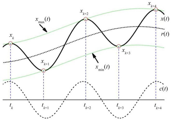
Figure 1.
The piece of signal x(t) as a signal analyzed.
Since c(t) is an oscillatory function with mean zero, its integral in the interval of two local maxima (or minima) points tk and tk + 2 should be equal to zero. Therefore, from Equation (1), one has
where ro(t) is the original function of r(t), that is, ro′(t) = r(t). Obviously, ro(t) is a real-valued function defined on interval [tk, tk + 2], and differentiable at every point on the interval, with continuity and a finite value of its derivative. According to the Lagrange differential theorem of mean, it is known that there is at least one point tl between tk and tk + 2 to make
Thus, Equation (2) can be rewritten as
Similarly, it can be derived that there is a point tm between tk+1 and tk+3 to make
Choosing a point C located at the central point from tk to tk + 1, as shown in Figure 2, can derive new relations from Equations (4) and (5), respectively, given by
where ∆t = (tk + 1 − tk)/2.
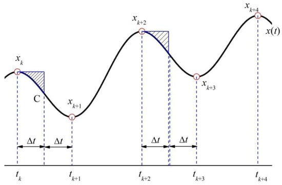
Figure 2.
Approximate to integrals over different intervals.
In order to introduce the values of extrema at four point tk, tk + 1, tk + 2, and tk + 3, one can use the following approximate relations
In Equation (8), ∆txk and ∆txk + 3 are approximate to two integrals of this equation, as shown in Figure 2. There are two shadow areas caused by this approximation. If they are almost equal to each other, such approximation is very good due to their difference considered here. Similarly, Equation (9) is also a good approximation when the other two areas in the integral calculation almost keep the same value. In Equation (10), the relevant two integrals have the same initial point, except for different end points. Both of them represent the integral means over their individual intervals with slight differences, and thus this equation should be a good approximation. Additionally, tm − tl approximated by 2 ∆t can be derived from the same step of movement for these two time points as that of their corresponding intervals.
With consideration of these approximate relations from Equations (8) to (11), subtracting Equation (7) divided by (tk + 3 − tk + 1) and Equation (6) divided by (tk + 2 − tk), after simplifying, yields
In Equation (12), the term on the left-hand side is approximate to the differential of r(t) with respect to time t, and the first and the second terms on the right-hand side are, respectively, to the differential of the curve xmax(t) between two local maxima and that of the curve xmin(t) between two local minima. With due regard to the behavior of r(t), xmax(t) and xmin(t) uniformly varying with time over the interval [tk, tk + 3], one has
Finally, one obtains
This equation shows that the trend r(t) in the decomposition expression (1) can be determined approximately by the mean of curves xmax(t) and xmin(t) generated by local maxima of the signal and local minima, respectively. Through Equation (1), the oscillation component c(t) can be computed so as to realize the decomposition of oscillation signal.
2.2. Basic Steps
- (1)
- Consider an oscillation signal x(t) varying with time t and take the piece of this signal as a signal analyzed. Assuming that this signal is composed of a pure oscillation component c(t) of proper rotation, with mean zero and a residual term (the trend or the baseline signal) r(t), Equation (1) follows.
- (2)
- Since c(t) integral in the interval of two local maxima (or minima) points tk and tk + 2 should be equal to zero. Equation (1) can be transformed into Equation (2).
- (3)
- According to the Lagrange differential theorem of mean, it is known that there is at least one point tl between tk and tk + 2 to make Equation (3). Thus, Equation (2) can be rewritten as Equation (4).It can be derived that there is a point tm between tk + 1 and tk + 3 to make Equation (5).
- (4)
- Choosing a point C located at the central point from tk to tk + 1, it can derive new relations from Equations (4) and (5). Equations (6) and (7) follow.
- (5)
- Where ∆t = (tk + 1 − tk)/2.
- (6)
- With consideration of these approximate relations from Equations (8) to (11), after simplifying, this yields Equation (12).
- (7)
- In Equation (12), the term on the left-hand side is approximate to the differential of r(t) with respect to time t, and the first and the second terms on the right-hand side. To the differential of the curve xmax(t) between two local maxima and that of the curve xmin(t) between two local minima. With due regard to the behavior of r(t), xmax(t), and xmin(t) uniformly varying with time over the interval [tk, tk + 3], one has Equation (13).
- (8)
- Finally, the component as in Equation (14) is obtained.
3. Characteristics of EMD Algorithm
The EMD algorithm, for a given signal x(t), generally contains following five steps or contents:
- (1)
- The successive extrema of x(t) are firstly identified, then the local maxima are connected by a cubic spline as the upper envelope, and the local minima are similarly connected as the lower envelope.
- (2)
- These two envelopes are used to calculate the mean as a function of time designated as m1(t).
- (3)
- The difference h1(t) between the signal x(t) and the mean m1(t) is calculated by the relation h1(t) = x(t) − m1(t), which can be regarded as the primary description of the first IMF.
- (4)
- To determine the first IMF more accurately, h1(t) is treated as a new signal, its upper and lower envelopes, and their new mean m2(t) are calculated, and a new difference h2(t) = h1(t) − m2(t) is determined. This h2(t) is again treated as a new signal, and the process, referred to as iteration, is repeated many times designated by k until a stopping criterion satisfies. hk(t) is the first IMF, designated by H1(t).
- (5)
- The first residue d1(t) = x(t) − H1(t) is analyzed by the same steps (1)–(4) to obtain the second IMF H2(t). This sifting process continues until the last residue shows no apparent variation.
3.1. Primary Description of the First IMF
In the EMD algorithm, the primary description of the first IMF is involved with the first three steps. It can be seen that two envelopes used to calculate the mean m1(t) correspond essentially to xmax(t) and xmin(t) in Equation (14), and the mean m1(t) is equal to the function r(t). Therefore, the theoretical principle of oscillation signal decomposition suggested above provides a theoretical basis available for the analysis of EMD.
It is noted to mention that, in deriving Equation (14), except for the assumption of xmax(t) and xmin(t) uniformly and continuously varying with time over the interval [tk, tk + 4], there are no other special requirements introduced. Obviously, these links can exclude the choice of straight lines due to the smooth property of r(t). Consequently, all nonlinear expressions should be appropriate for the links between the nearest maxima or between the nearest minima only if they meet the requirement of varying with time uniformly and smoothly, which can explain this phenomenon that it is very difficult to agree in the best implementation for so many studies.
3.2. Iteration and Sifting Process
Because primary description of the first IMF cannot determine the first IMF more accurately, it is necessary to operate the iteration calculation by following the step (4). In fact, the decomposition relation of Equation (14) is just an approximate expression. An important question is whether the EMD algorithm based on the suggested theoretical principle of oscillation signal decomposition can reach the decomposition result described by Equation (1) through the iteration process.
Up to this date, there has not been a direct convergence proof of the iteration process, even though using trigonometric interpolation, instead of cubic splines, in the extraction process, shows a good convergence [22]. Worthy of note, the primary description of the first IMF generally indicates the extrema positions of the oscillation component c(t) searched further, which should be very useful information for the convergence proof of the iteration process.
The primary description of the first IMF can be expressed as c(0)(t). Assuming that the extrema positions of c(0)(t) represent the real extrema positions of the oscillation component c(t), and taking one of them as the point analyzed at which the extremum is Ma and the value of another curve linking the maxima or minima is Mb, may yield, after the first iteration, that the corresponding mean (or trend) r(1) can be calculated by means of Equation (14) and expressed as
The value of oscillation component c(1) is calculated through Equation (1), given by
After the second iteration, the mean r(2) and the oscillation value c(2) are given by
where is the value of the curve linking the other two neighbor extrema at the position of previous extremum considered. After the third iteration, the mean r(2) and the oscillation value c(2) are given by
where is the value of the curve linking the other two neighbor extrema. After the jth iteration, one has
Since (l = 1, 2, 3, …, j − 1) are finite, there is a positive amount M satisfying , and Equation (19) can be rewritten as
When j→∞, one has r(j)→0. This result can be derived from any one of the extrema positions of c(0)(t). Since the function r(t) varies monotonically on most of the intervals between two neighbor extrema, it can be seen that r(j)→0 at all extrema means that the approximate function r(t) calculated by Equation (14), after many iterations, tends to zero at every time point, that is
Therefore,
This result shows that the EMD algorithm has good robustness.
After the oscillation component c(t) is extracted from the original signal, the remaining content, the trend r(t) may still represent an oscillation signal. At this time, it is necessary for a complete decomposition to run a sifting process to get the other oscillation components until the last remaining content shows no apparent variation.
So, when the frequencies of the two signals are close to twice the range, the EMD method does not separate the two signals well.
4. Analysis and Discussion
For a long time, the method of EMD has been faced with the difficulty of being essentially defined by an algorithm, and therefore of not admitting an analytical formulation which would allow for a theoretical analysis and performance evaluation. To this end, a better understanding of this method is presented by the suggested theoretical principle of oscillation signal decomposition as follows.
4.1. Interpolation
Interpolation in EMD is concerned with two problems of the best spline implementation and the optimum positions of the interpolation points. It can be seen from the construction of the theoretical principle that there is essentially not a best spline implementation. However, the upper envelope or the lower envelope shooting the inner signal may seriously spoil the requirement that the link line between the nearest two minima or maxima varies with time uniformly and smoothly, and so does that bulging away from the signal. When signals with different characteristics are analyzed, different spline implementations can be chosen and the same result can be obtained only if the condition of uniform and smooth variation between two nearest local minima or maxima is satisfied. In order to meet the condition more effectively, xmax(t) and xmin(t) had best to monotonically vary with time on the intervals between two nearest maxima or minima [23].
The positions of the interpolation points can cause the approximation degree of Equations (8) and (9). If the extrema are set to the most proper positions, the decomposition performance of EDM is able to be much improved [13]. However, on the basis of the suggested theoretical principle, it has not been found an available way for the detection of the optimum positions of the interpolation points.
4.2. Frequency Resolving Ability
Whether in determining the upper envelope or the lower envelope, at least three corresponding local extrema points are used, which shows that the oscillation component can be extracted, in the case of the total number of extrema more than six, from the piece of signal. It is well known that three extrema cover a periodic time of the oscillation. This is to say, the theoretical limit that the EMD can accurately distinguish the difference between two oscillation components is the periodical difference more than two times or less than half of a time, or the frequency ratio up to 2 or less than 0.5. This should be a common knowledge related to the method of EMD. However, some investigations found that the actual separable range occurs between two oscillation components with frequency ratio larger than 1/0.6 and less than 0.6 [16,17,24].
In fact, Equation (14) shows that four successive extrema can only provide the information of r(t) on the interval between tl and tm. This interval is not sure to cover the periodic time of the oscillation component, an interval with three successive local extrema of the signal. Thus, it is necessary to add the piece of signal up to next extremum into the signal analyzed. That is to say, decomposing the oscillation component described by three extrema requires the piece of signal, at least, with five extrema. It shows that the theoretical limit of frequency resolving ability of EMD is just the frequency ratio larger than 1/0.6 and less than 0.6, while the frequency ratio more than 2 or less than 0.5 should be its optimum frequency resolving ability. To break through this theoretical limit, a number of approaches have been made so far, all showing their advantage in reducing the so-call mode mixing [3,18,20,21]. Unfortunately, evidence provided by the suggested theoretical principle has led to fruitless efforts, essentially, that the EMD is modified under the present framework.
When the extrema considered in Figure 1 are expanded to point xk+4, a relation similar to Equations (4) or (5) on the interval [xk + 2, xk + 4] can be added as
where tn is a point in the interval (xk+2, xk+4). Generally, one has, tl < tm < tn. It can be found that the data set {(tl, r(tl )); (tm, r(tm)); (tn, r(tn)} provides interpolation points for the solution of r(t) by means of the spline implementation. Since only five local extrema points are used, the interpolation solution makes the frequency resolving ability increase to the range of the frequency ratio larger than 5/3 and less than 3/5, which just corresponds to the actual limitation of the EMD. However, tl, tm and tn are unknown to operate this decomposition. The method of EMD makes full use of the information associated with extrema of the signal and coincidently avoids the difficulty to determine parameters tl, tm and tn at the cost of lowering its frequency resolving ability.
In the interpolation solution, each time point such as tl, tm, and tn can roughly be taken as the centre of its corresponding time interval. Figure 3 presents the decomposition results of two digital simulation signals with two components. One simulation signal has frequency ratio 3, and another 1.4. Comparing with the results obtained by the EMD, one can see that results from the interpolation solution are not better than those from the EMD for lack of optimal interpolation time estimates, but the former can obviously increase the frequency-resolving ability of oscillation signal decomposition, which should indicate a developing direction for reducing the mode mixing of EMD.
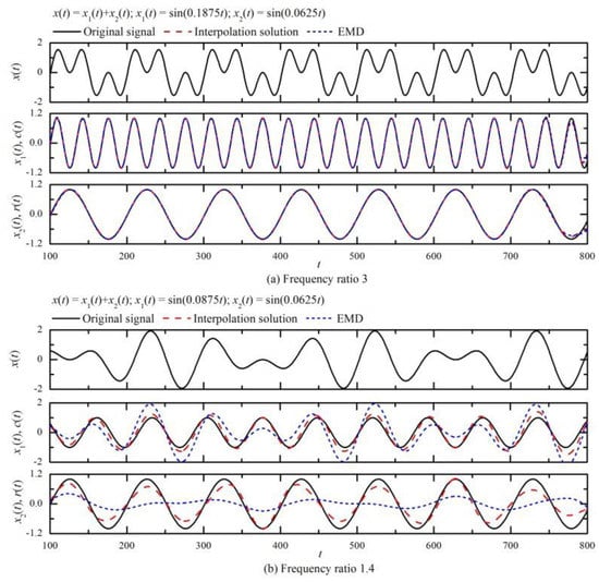
Figure 3.
Comparison of decomposition results between interpolation solution and empirical mode decomposition (EMD).
4.3. Assumption and Approximation in the Theoretical Principle
Once there are several tl on the interval (xk, xk + 2), tm on (xk + 1, xk + 3), or tn on (xk + 2, xk + 4) (impossible for all of them to occur simultaneously), Equations (12) and (13) simultaneously turn the exact relations into approximate expressions, which means that the central point of several tl, tn, or tm, or any one of them can also work well. Since the interval considered moves by a step of a half wave length, this relationship tl < tm < tn is always following. Examples of interpolation solution decomposition, as shown in Figure 3, illustrate that tl, tm, and tn should be located near the centre of their corresponding intervals. Affirmatively, more than one tl, tm, or tn will have influence on the effect of interpolation solution decomposition, but have little on the EMD.
Equation (12) is associated with several approximate relations given by Equations (8) to (11). Since they are easily accepted in applications to present reasonable approximate expressions, Equation (13) is derived. Frankly, only when xmax(t), xmin(t), and r(t) are very close to straight lines over the interval (tl, tm), can the approximation involved in this equation be correct. The upper envelope generated by local maxima of a signal and the lower one by local minima can be controlled properly to describe the link between two nearest maxima or minima close to a straight line. Naturally, r(t) close to a straight line can be regarded. One cannot adopt the assumption that the segments of two envelopes between two nearest maxima and minima are straight lines, because straight lines cannot cover the signal well and also cannot portrait its property smoothly varying with time. In view of this, Equation (13) is an inevitable inference drawn from Equation (12).
The robustness of the EMD algorithm shows that whether any assumption or simplification is introduced into the relation of Equation (14), a satisfactory decomposition effect can be obtained if the primary description of the first IMF, calculated by the result from this relation, has correct characteristic information. This characteristic information completely depends on its time locations of the local extrema. Iteration process is essentially to remove errors caused by the approximation express of Equation (14) by means of the constraints between neighbor waves.
4.4. Bearing Fault Data Analysis
In order to further verify the adaptive advantages of the empirical mode decomposition algorithm, this experiment will analyze the bearing fault data. The experimental data comes from the Case Fault Database of Case Western Reserve University [25]. The fault signal of the inner ring of the drive end is selected to analyze the feature of the EMD method, and compared with the application effect of the wavelet method. Specific experimental procedures are detailed in References [26,27,28]. The experimental conditions are as follows: the drive end bearing adopts 6205-2RS JEM SKF deep groove ball bearing, EDM bearing single point damage, the damage diameter is 0.1778 mm, the motor speed is 1748 r/min, the sampling frequency is 12 KHz, the sampling time is 0.25 s (107.dat). The inner ring fault frequency can be theoretically calculated to be 157.8 Hz. The time domain waveform of the measured signal is shown in Figure 4. The spectrum of the waveform shown in Figure 4 is shown in Figure 5.
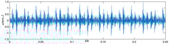
Figure 4.
Inner ring fault bearing data time domain waveform diagram.
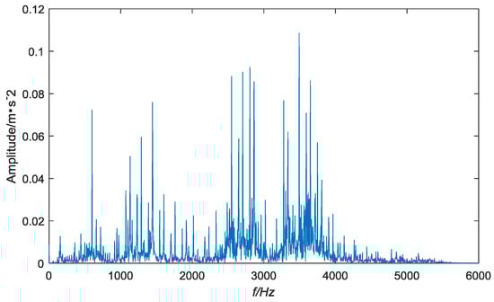
Figure 5.
Spectrum diagram of Figure 4.
As shown in Figure 5 that the bearing inner ring produces localized periodic characteristics of the disturbing vibration signal, and there are a large number of peak groups in the low frequency part of the spectrum, so the bearing failure type cannot be judged.
In order to better analyze the characteristics of the EMD method, the bearing inner ring fault signal shown in Figure 4 is decomposed by EMD and wavelet respectively, and the results are shown in Figure 6 and Figure 7.
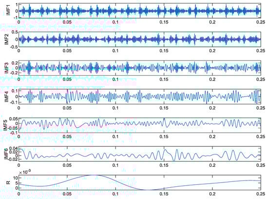
Figure 6.
EMD method decomposition result graph.
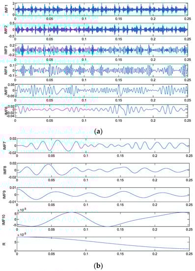
Figure 7.
Wavelet method decomposition result graph.
It can be seen from Figure 6 and Figure 7 that the EMD method only decomposes and obtains 7 IMF components, while the wavelet method decomposes to obtain 11 IMF components, and the 11 IMF components have redundant components. The main reason for this situation is that the wavelet method itself is not adaptive, its decomposition process is largely affected by the wavelet basis, and the EMD algorithm has a high degree of adaptive characteristics, which can be completely decomposed according to the characteristics of the signal itself.
The instantaneous frequency distribution of the first six natural modal components obtained by EMD and wavelet decomposition is shown in Figure 8 and Figure 9. It can be known that the instantaneous frequency distribution of the first six natural modal components obtained by EMD decomposition has no obvious frequency crossover and aliasing. The instantaneous frequency distribution of the first six modal components obtained by wavelet decomposition has extremely obvious frequency crossover and aliasing. In other words, the EMD method better solves the pattern aliasing problem.
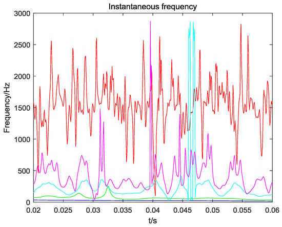
Figure 8.
Instantaneous frequency distribution of component parts obtained by EMD method decomposition.
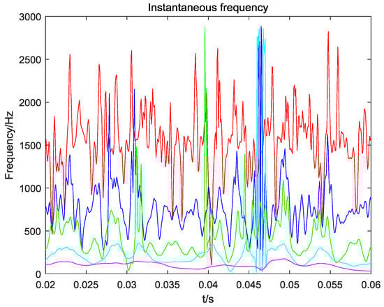
Figure 9.
Instantaneous frequency distribution of component parts obtained by wavelet method decomposition.
In order to further reflect the adaptability and superiority of the EMD method, the fault feature frequency extraction capabilities of the wavelet and EMD methods are compared. The FFT operation is performed on the relevant modal components obtained by the above two methods, and the results are shown in Figure 10 and Figure 11. It can be seen from Figure 10 that after the inner ring signal of the above rolling bearing is decomposed by wavelet, the fault frequency appears in two adjacent modal components of IMF5 and IMF6, and the amplitude is large, and the modal aliasing phenomenon is serious. It has a great interference to the accurate extraction of the inner ring fault vibration signal characteristics. It can be seen from Figure 11 that after the inner circle signal is decomposed by the EMD. The fault frequency can only be found in the IMF4 component, and the interference frequency is small. It can be clearly seen that its peak value should be the inner loop fault characteristic frequency, which is about 156 Hz (subject to the actual environment, it may be slightly different from the theoretical value). It can be known from the above analysis that the fault characteristic frequency extraction ability of the EMD method is strong, and it can be effectively applied to the feature extraction analysis of the inner ring fault of the rolling bearing.
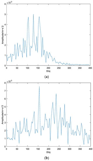
Figure 10.
Partial modal component spectrum obtained by wavelet decomposition. (a) IMF5 component spectrum, (b) IMF6 component spectrum.
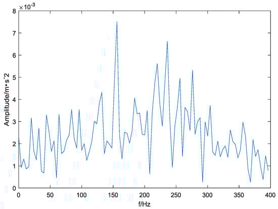
Figure 11.
IMF4 component spectrum obtained by EMD decomposition.
Although the wavelet method does not accurately find the fault frequency, it probably determines the range of the fault frequency. This is the effect of the EMD method and the wavelet method on the decomposition of the vibration data. In order to compare with the traditional FFT method, the data used in this experiment is analyzed by FFT, and the results are shown in Figure 12. It can be seen from Figure 12 that the frequency spectrum of the inner ring signal obtained by the FFT transform cannot find the fault frequency of the inner loop signal. It is even more difficult to accurately obtain the specific value of the fault signal frequency. It can also be seen that there is a certain gap between the FFT method and the smaller wave method, and there is a larger gap than the EMD.
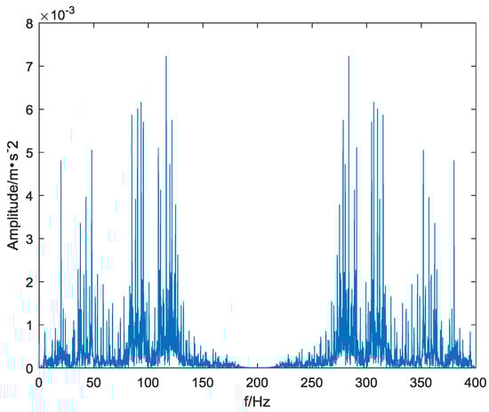
Figure 12.
Fault signal FFT spectrum.
At the same time, in order to further verify the effectiveness and reliability of the EMD method for noise-containing fault signal processing, random noise is added to the inner-circle fault signal in this experiment, as shown in Figure 13. The wavelet signal and the EMD method are used to denoise the noisy signal of Figure 13, and the results are shown in Figure 14 and Figure 15. It can be seen from Figure 14 and Figure 15 that the EMD method can better eliminate noise, and although the wavelet method also eliminates part of the noise, there is still significant noise information. The signal-to-noise ratio and root mean square error after noise removal by the two methods are shown in Table 1. It can be seen that the signal denoised by the EMD method, whether it is the signal-to-noise ratio or the root mean square error, is more advantageous than the signal after the wavelet method is denoised. At the same time, the computational efficiency of the EMD method is higher than that of the FFT method and the wavelet method. This is because the IMF component obtained by EMD decomposition is more favorable for later analysis.
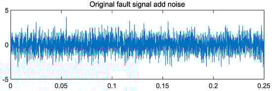
Figure 13.
Inner circle signal plus random noise effect diagram.

Figure 14.
Wavelet method denoising effect diagram.
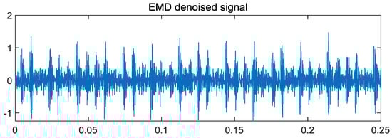
Figure 15.
EMD method denoising effect diagram.

Table 1.
Comparison of SNR and RMSE after denoising by EMD and wavelet method.
5. Conclusions
This work firstly presents a mathematical proof for the validity and robustness of the method of EMD, which may provide a primary theoretical framework available for the development of EMD.
A piece of oscillation signal with four local extrema is considered, and a theoretical principle of the oscillation signal decomposition is suggested, based on the requirement of a pure oscillation component with mean zero extracted from it. Through some approximations, the general calculation formula used in the EMD algorithm is derived. The trend in the decomposition expression can be determined approximately by the mean of two curves generated by local maxima of the signal and local minima, respectively. It seems that all nonlinear expressions should be appropriate for the links between the nearest maxima or minima, if they meet the requirement varying with time uniformly and smoothly. When the extrema are set to the most proper positions, the decomposition performance of EMD is able to be much improved
According to the movement of any one local extremum point involved in the primary description of the first IMF in the iteration process, it can be found that the residual tends to zero with the increase of iteration times. With consideration of the property of the trend function varying monotonically over the interval between almost all of two nearest neighbor extrema, the convergence of iteration process is demonstrated exactly. This result shows that the EMD algorithm has good robustness.
Simulation experiments show that the proposed method has good adaptive characteristics and high resolution. At the same time, for the noise-carrying rolling bearing signal, the EMD method and the wavelet method are used to denoise respectively, and the EMD method smaller wave method has better denoising effect. The example analysis results of the fault vibration signal of the inner ring of rolling bearing show that the correlation coefficient of each modal component in the result of decomposition by this method is high. Compared with the wavelet method, the method extracts the effective diagnostic information and feature information hidden in the fault vibration signal of the inner ring of the complex bearing, which highlights the fault frequency of the inner ring of the bearing. The EMD method and the wavelet method can obtain the fault signal frequency information more than the traditional FFT method.
The suggested theoretical principle of the oscillation signal decomposition proposes the possibility for constructing a modified version of EMD through the interpolation solution, to improve the frequency resolving ability. However, it is an unsolvable problem to properly determine some time parameters in each periodical oscillation starting at any one extremum point. The method of EMD makes full use of the information associated with extrema of the signal and coincidently avoids this difficulty at the cost of lowering its frequency resolving ability. The decomposition test of two simulation signals, composed by two oscillation components with frequency ratio 3 and 1.4, shows that results from the interpolation solution are not certainly better than those from the EMD due to lack of optimal interpolation time estimates, but the former can obviously increase the frequency resolving ability of oscillation signal decomposition, which should indicate a developing direction for reducing the mode mixing effect of EMD. Additionally, some approximations in deriving the general calculation formula used in the EMD algorithm are briefly analyzed and discussed.
Author Contributions
Conceptualization, H.G. and G.C.; Methodology, F.A.; Software, H.G. and F.A.; Validation, H.G., H.Y., and H.C.; Formal Analysis, H.G.; Investigation, G.C.; Resources, F.A. and H.Y.; Data Curation, H.G.; Writing-Original Draft Preparation, H.G. and F.A.; Writing-Review & Editing, G.C.; Supervision, H.Y.; Project Administration, H.G.; Funding Acquisition, H.G.
Funding
This work received no specific grant from any funding agency in the public, commercial, or not-for-profit sectors.
Acknowledgments
This work was supported by the University–industry cooperation prospective project of Jiangsu Province: Development of intelligent universal color-selecting and drying grain machine (BY2016062-01).
Conflicts of Interest
The authors declare no conflict of interest.
References
- Huang, N.E.; Shen, Z.; Long, S.R.; Wu, M.L.; Shih, H.H.; Zheng, Q.; Yen, N.C.; Tung, C.C.; Liu, H.H. The empirical mode decomposition and Hilbert spectrum for nonlinear and non-stationary time series analysis. Proc. R. Soc. Lond. A 1998, 454, 903–995. [Google Scholar] [CrossRef]
- Rilling, G.; Flandrin, P.; Goncalves, P. On empirical mode decomposition and its algorithms. In Proceedings of the IEEE-EURASIP Workshop on Nonlinear Signal and Image Processing NSIP-03, Grado, Italy, 8–11 June 2003. [Google Scholar]
- Lee, Y.S.; Tsakirtzis, S.; Vakakis, A.F.; Bergman, L.A.; McFarlan, D.M. Physics-based foundation for empirical mode decomposition. AIAA J. 2009, 47, 2938–2963. [Google Scholar] [CrossRef]
- Feldman, M. Hilbert transform in vibration analysis. Mech. Syst. Signal Process. 2011, 25, 735–802. [Google Scholar] [CrossRef]
- Yang, J.N.; Lei, Y.; Pan, S.; Huang, N.H. System identification of linear structures based on Hilbert-Huang spectral analysis, part 1: Normal modes. Earthq. Eng. Struct. Dyn. 2003, 32, 1443–1467. [Google Scholar] [CrossRef]
- Yang, J.N.; Lei, Y.; Pan, S.; Huang, N.H. System identification of linear structures based on Hilbert-Huang spectral analysis, part 2: Complex modes. Earthq. Eng. Struct. Dyn. 2003, 32, 1533–1554. [Google Scholar] [CrossRef]
- Pai, P.F. Time–frequency characterization of nonlinear normal modes and challenges in nonlinearity identification of dynamical systems. Mech. Syst. Signal Process. 2011, 25, 2358–2374. [Google Scholar] [CrossRef]
- Lee, Y.S.; Vakakis, A.F.; McFarland, D.M.; Bergman, L.A. A global-local approach to nonlinear system identification: A review. Struct. Control Health Monit. 2010, 17, 742–760. [Google Scholar] [CrossRef]
- Li, H.; Deng, X.; Dai, H. Structural damage detection using the combination method of EMD and wavelet analysis. Mech. Syst. Signal Process. 2007, 21, 298–306. [Google Scholar] [CrossRef]
- Liu, B.; Riemenschneider, S.; Xu, Y. Gearbox fault diagnosis using empirical mode decomposition and Hilbert spectrum. Mech. Syst. Signal Process. 2006, 20, 718–734. [Google Scholar] [CrossRef]
- Gao, Q.; Duan, C.; Fan, H.; Meng, Q. Rotating machine fault diagnosis using empirical mode decomposition. Mech. Syst. Signal Process. 2008, 22, 1072–1081. [Google Scholar] [CrossRef]
- Ricci, R.; Pennacchi, P. Diagnostics of gear faults based on EMD and automatic selection of intrinsic mode functions. Mech. Syst. Signal Process. 2011, 25, 821–838. [Google Scholar] [CrossRef]
- Kopsinis, Y.; McLaughlin, S. Investigation and performance enhancement of the empirical mode decomposition method based on a heuristic search optimization approach. IEEE Trans. Signal Process. 2008, 56, 1–13. [Google Scholar] [CrossRef]
- Deléchelle, E.; Lemoine, J.; Niang, O. Empirical mode decomposition: An analytical approach for sifting process. IEEE Signal Process. Lett. 2005, 12, 764–767. [Google Scholar] [CrossRef]
- Niang, O.; Deléchelle, E.; Lemoine, J. A spectral approach for sifting process in empirical mode decomposition. IEEE Trans. Signal Process. 2010, 58, 5612–5623. [Google Scholar] [CrossRef]
- Rilling, G.; Flandrin, P. One or two frequencies? The empirical mode decomposition answers. IEEE Trans. Signal Process. 2008, 56, 85–95. [Google Scholar] [CrossRef]
- Feldman, M. Analytical basics of the EMD: Two harmonics decomposition. Mech. Syst. Signal Process. 2009, 23, 2059–2071. [Google Scholar] [CrossRef]
- Huang, N.E.; Shen, Z.; Long, S.R. A new review of nonlinear water waves: The Hilbert spectrum. Ann. Rev. Fluid Mech. 1999, 31, 417–457. [Google Scholar] [CrossRef]
- Smith, J.S. The local mean decomposition and its application to EEG perception data. J. R. Soc. Interface 2005, 2, 443–454. [Google Scholar] [CrossRef] [PubMed]
- Hong, H.; Wang, X.; Tao, Z. Local integral mean-based sifting for empirical mode decomposition. IEEE Signal Process. Lett. 2009, 16, 841–844. [Google Scholar] [CrossRef]
- Li, C.; Wang, X.; Tao, Z.; Wang, Q.; Du, S. Extraction of time varying information from noisy signals: An approach based on the empirical mode decomposition. Mech. Syst. Signal Process. 2011, 25, 812–820. [Google Scholar] [CrossRef]
- Hawley, S.D.; Atlas, L.E.; Chizeck, H.J. Some properties of an empirical mode type signal decomposition algorithm. IEEE Signal Process. Lett. 2010, 17, 24–27. [Google Scholar] [CrossRef]
- Xu, Z.; Huang, B.; Li, K. An alternative envelope approach for empirical mode decomposition. Digit. Signal Process. 2010, 20, 77–84. [Google Scholar] [CrossRef]
- Datig, M.; Schlurmann, T. Performance and limitations of the Hilbert-Huang transformation (HHT) with an application to irregular water waves. Ocean Eng. 2004, 31, 1783–1834. [Google Scholar] [CrossRef]
- Case Western Reserve University Data Center. Available online: https://csegroups.case.edu/bearingdatacenter/home (accessed on 9 November 2018).
- Dang, Z.; Lv, Y.; Li, Y.; Wei, G. Improved Dynamic Mode Decomposition and Its Application to Fault Diagnosis of Rolling Bearing. Sensors 2018, 18, 1972. [Google Scholar] [CrossRef] [PubMed]
- Pang, B.; Tang, G.; Tian, T.; Zhou, C. Rolling Bearing Fault Diagnosis Based on an Improved HTT Transform. Sensors 2018, 18, 1203. [Google Scholar] [CrossRef] [PubMed]
- Wan, S.; Zhang, X. Teager Energy Entropy Ratio of Wavelet Packet Transform and Its Application in Bearing Fault Diagnosis. Entropy 2018, 20, 388. [Google Scholar] [CrossRef]
© 2018 by the authors. Licensee MDPI, Basel, Switzerland. This article is an open access article distributed under the terms and conditions of the Creative Commons Attribution (CC BY) license (http://creativecommons.org/licenses/by/4.0/).