Interactive Cutting of Thin Deformable Objects


Abstract
1. Introduction
2. Related Works
2.1. Simulation of Deformable Bodies
2.2. Collision Handling for Thin Deformable Bodies
2.3. Cutting for Deformable Objects
2.3.1. Cutting of Conformal Mesh
2.3.2. Cutting of Multi-Resolution Mesh
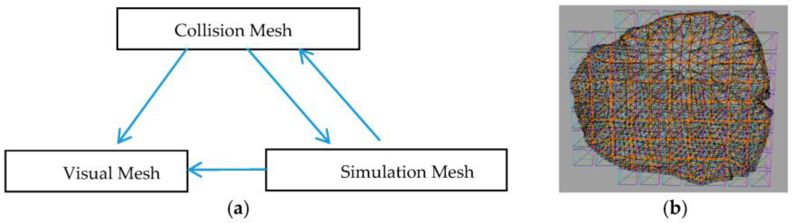
3. Research Hypothesis and Overview
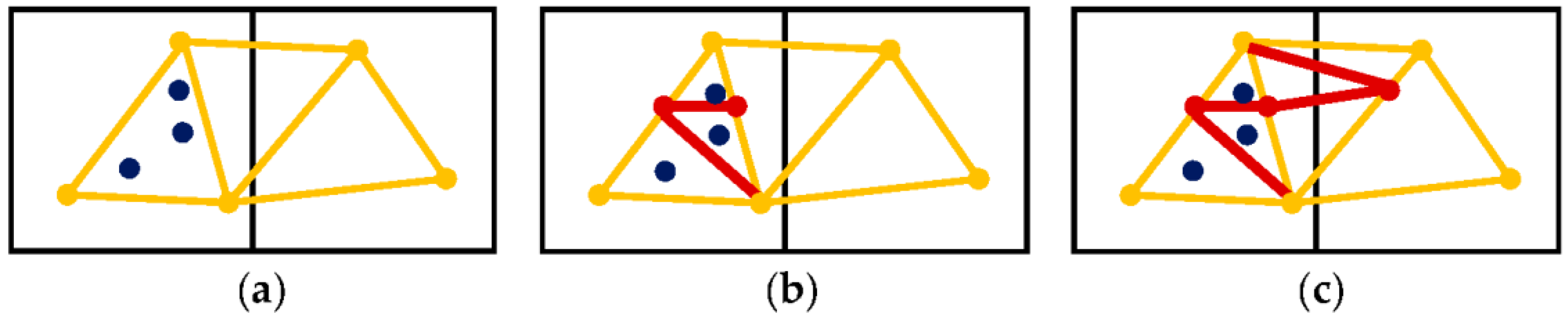
- Cutting of collision mesh. The cutting blade is intersected with the collision mesh. The triangles are split along the path of the blade.
- Cutting of visual mesh. Based on the visual-collision binding, the visual mesh is cut in the rest configuration using local 2D coordinates. Then, the visual-collision binding is updated.
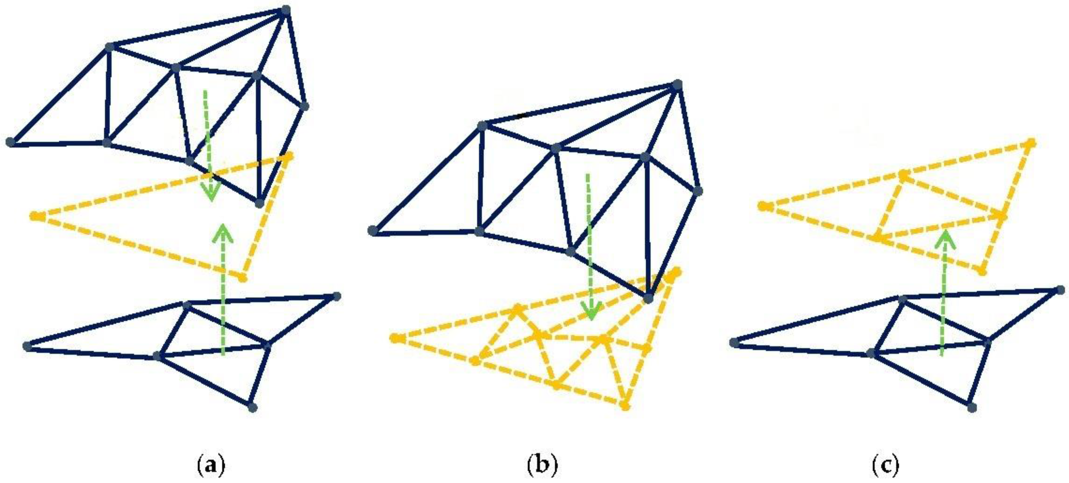
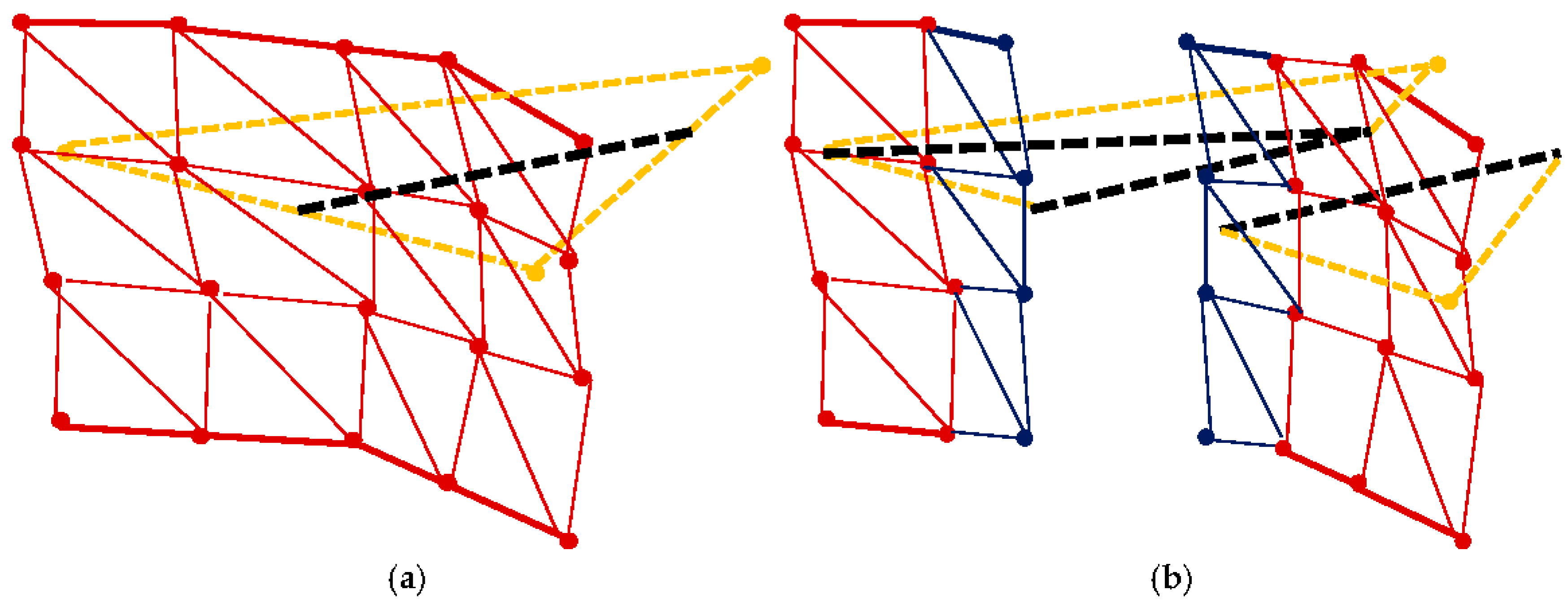
- Simulation mesh adapting to the cut. The branches of the collision mesh contained in the elements of the simulation mesh are analyzed. The elements are duplicated for each branch. The collision-simulation embedding is updated.
- Updating the visual-simulation embedding. According to the visual-collision binding, the visual-simulation embedding is updated.
4. Method
4.1. Pre-Processing Phase
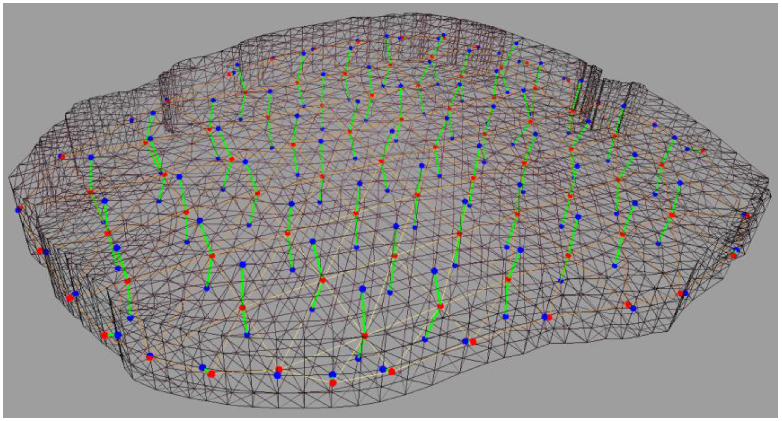
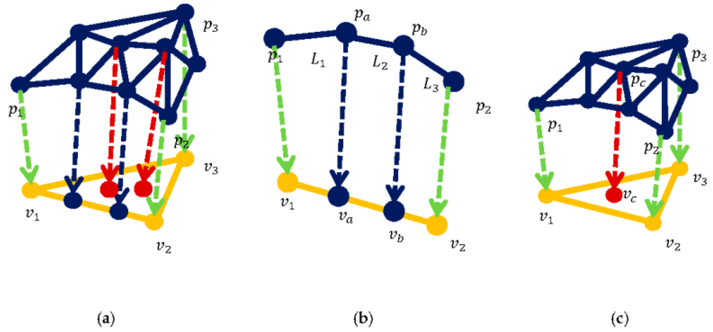
4.1.1. Bind Visual Vertices to Collision Vertices
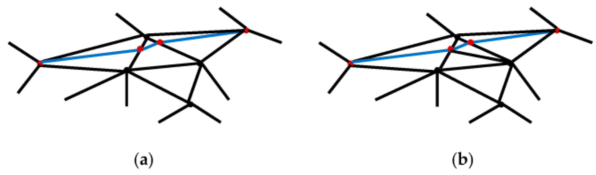
4.1.2. Calculate Geodesic Paths between the Bound Visual Vertices
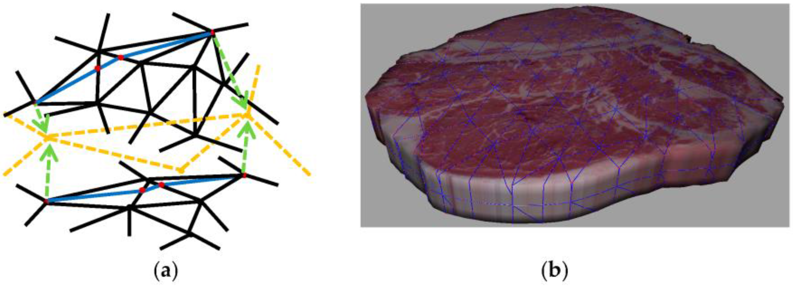
4.1.3. Re-Meshing of the Visual Mesh
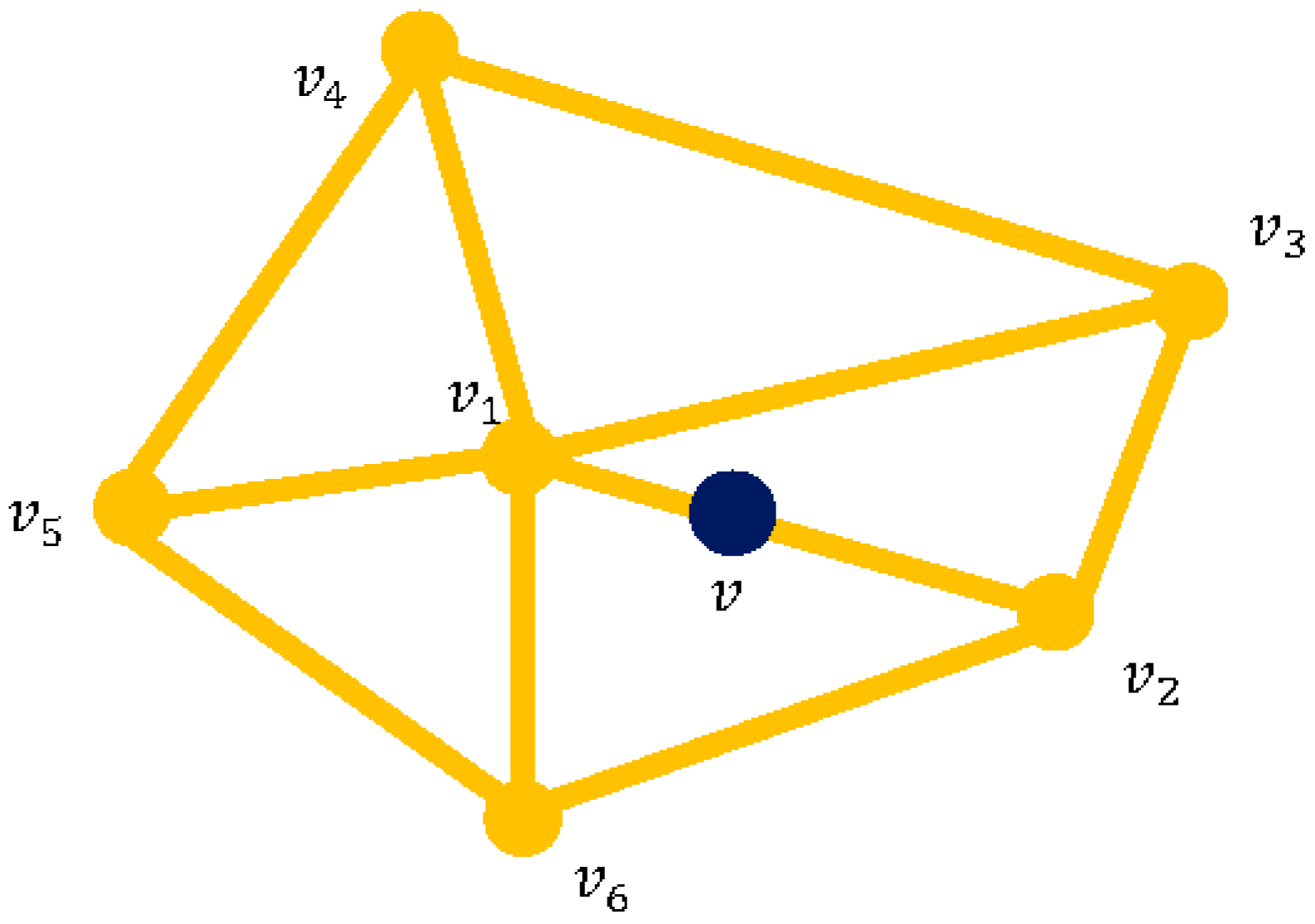
4.1.4. Assigning Local Parameters to the Visual Vertices
4.2. Simulation Phase
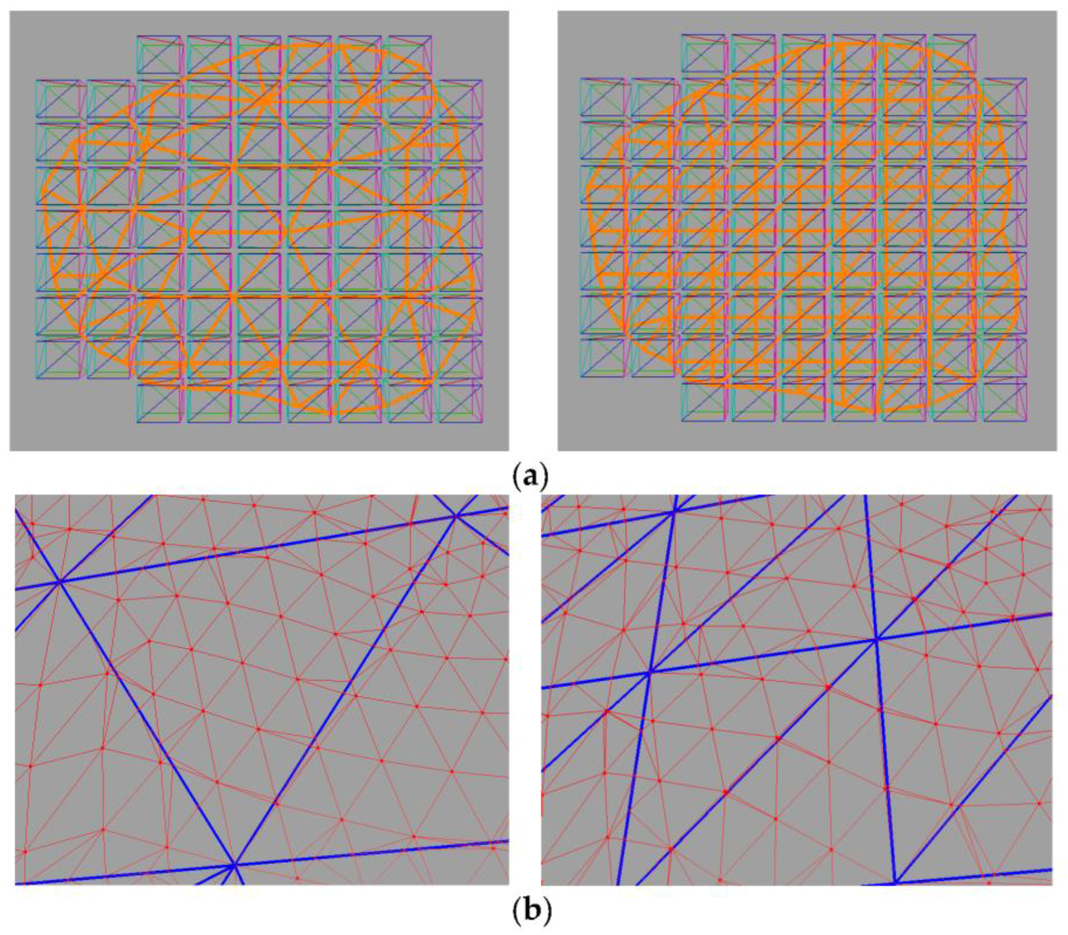
4.2.1. Cutting the Collision Mesh and Updating the Collision-Simulation Embedding
4.2.2. Cutting the Visual Mesh
4.2.3. Updating the Visual-Collision Binding
4.2.4. Handling the Cut Surface Mesh
4.2.5. Updating the Visual-Simulation Embedding
5. Experimental Results
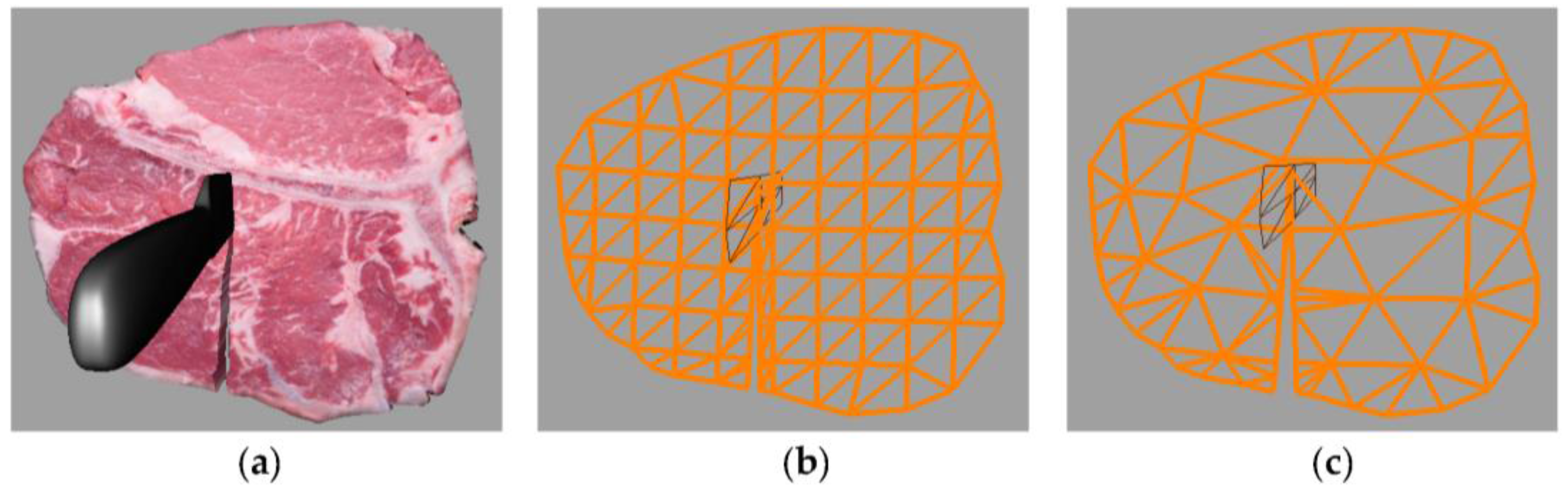
5.1. Cutting of a Steak
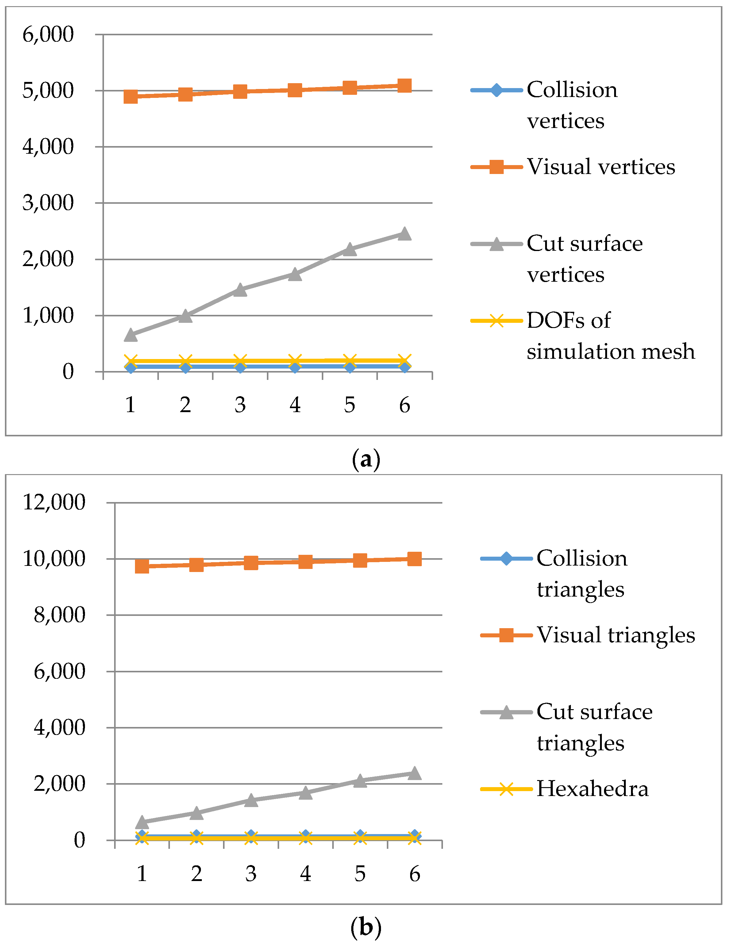
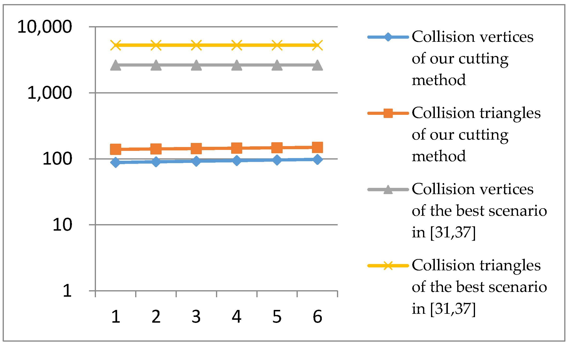
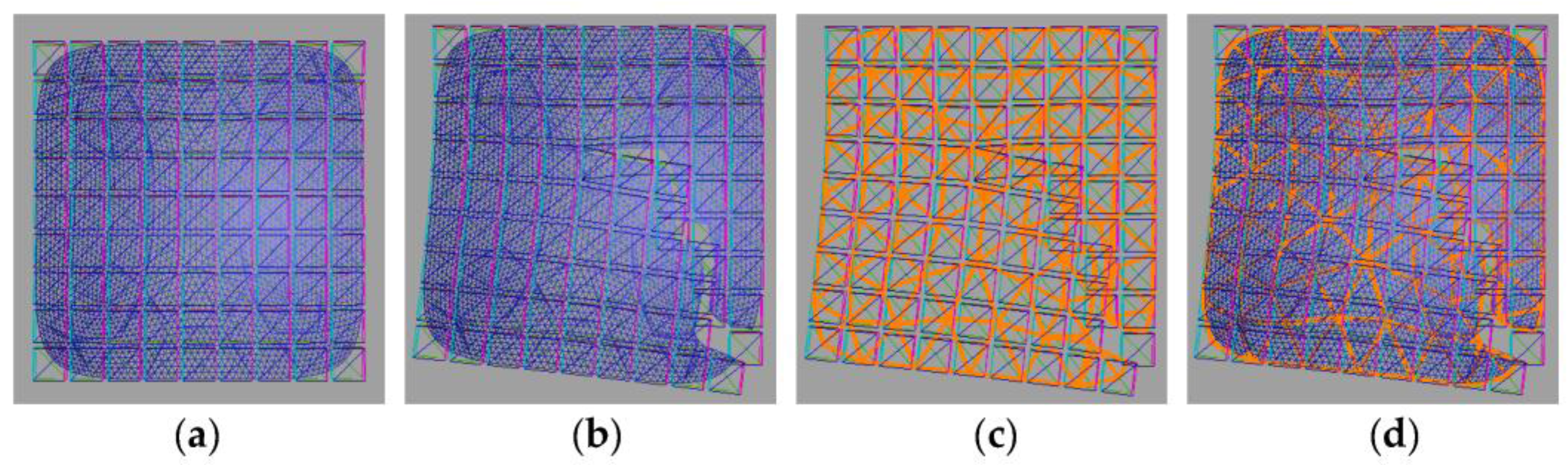
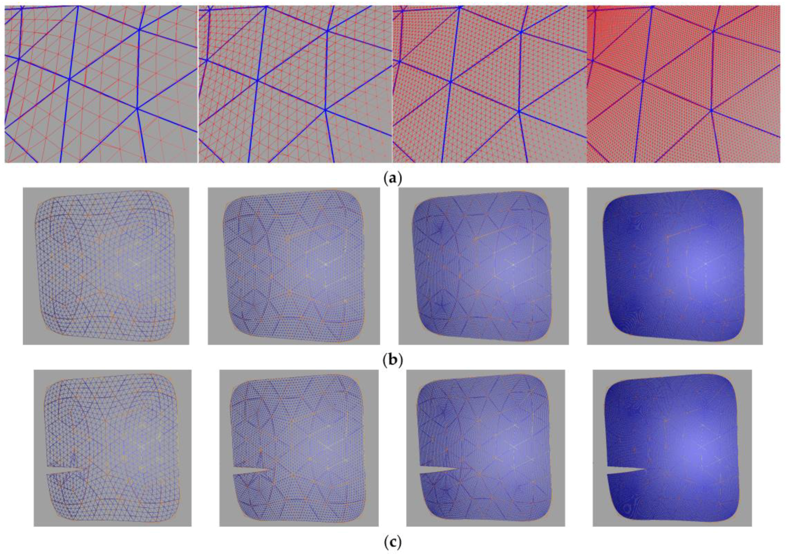
5.2. Cutting of a Thin Object
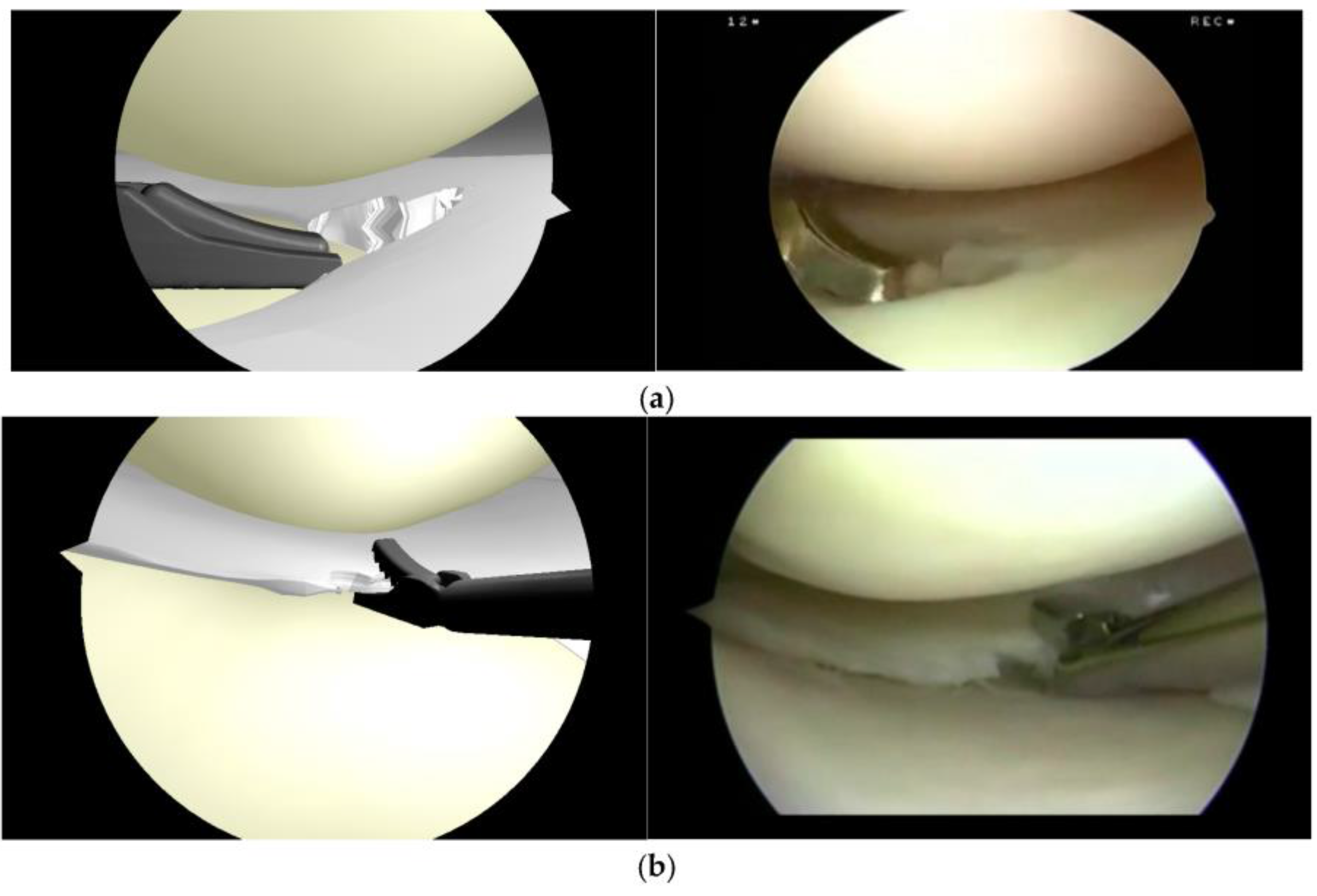
5.3. Meniscus Lesion Handling in a Prototype Simulator
6. Conclusions
Supplementary Materials
Acknowledgments
Author Contributions
Conflicts of Interest
References
- Spillmann, J.; Harders, M. Robust Interactive Collision Handling between Tools and Thin Volumetric Objects. IEEE Trans. Vis. Comput. Graph. 2012, 18, 1241–1254. [Google Scholar] [CrossRef] [PubMed]
- Wu, J.; Westermann, R.; Dick, C. A Survey of Physically Based Simulation of Cuts in Deformable Bodies. Comput. Graph. Forum 2015, 18, 161–187. [Google Scholar] [CrossRef]
- Terzopoulos, D.; Platt, J.; Barr, A.; Fleischer, K. Elastically deformable models. ACM Siggraph Comput. Graph. 1987, 21, 205–214. [Google Scholar] [CrossRef]
- Maciej, K.; Hiroshi, N. Mass spring models with adjustable Poisson’s ratio. Vis. Comput. 2017, 33, 283–291. [Google Scholar]
- Yeung, Y.H.; Crouch, J.; Pothen, A. Interactively Cutting and Constraining Vertices in Meshes Using Augmented Matrices. ACM Trans. Graph. 2016, 35, 1–17. [Google Scholar] [CrossRef]
- Fihai, F.; Florica, M. Position based simulation of solids with accurate contact handling. Comput. Graph. 2017, 69, 12–23. [Google Scholar]
- Berndt, I.; Torchelsen, R.; Maciel, A. Efficient Surgical Cutting with Position-Based Dynamics. IEEE Comput. Graph. Appl. 2017, 38, 24–31. [Google Scholar] [CrossRef] [PubMed]
- Sifakis, E.; Barbic, J. FEM simulation of 3D deformable solids: A practitioner’s guide to theory, discretization and model reduction. In Proceedings of the ACM SIGGRAPH 2012 Courses, Los Angeles, CA, USA, 5–9 August 2012; ACM: New York, NY, USA, 2012; pp. 1–50. [Google Scholar]
- Teschner, M.; Kimmerle, S.; Heidelberger, B. Collision Detection for Deformable Objects. Comput. Graph. Forum 2005, 24, 61–81. [Google Scholar] [CrossRef]
- Cotin, S.; Delingette, H.; Ayache, N. A hybrid elastic model for real-time cutting, deformations, and force feedback for surgery training and simulation. Vis. Comput. 2000, 16, 437–452. [Google Scholar] [CrossRef]
- Courtecuisse, H.; Allard, J.; Kerfriden, P. Real-time simulation of contact and cutting of heterogeneous soft-tissues. Med. Image Anal. 2014, 18, 394–410. [Google Scholar] [CrossRef] [PubMed]
- Bielser, D.; Maiwald, V.A.; Gross, M.H. Interactive Cuts through 3-Dimensional Soft Tissue. Comput. Graph. Forum 1999, 18, 31–38. [Google Scholar] [CrossRef]
- Nienhuys, H.W.; Frank van der Stappen, A. A Surgery Simulation Supporting Cuts and Finite Element Deformation. In Proceedings of the International Conference on Medical Image Computing and Computer-Assisted Intervention—MICCAI 2001, Utrecht, The Netherlands, 14–17 October 2001; Niessen, W., Viergever, M., Eds.; Springer: Berlin/Heidelberg, Germany, 2001; pp. 145–152. [Google Scholar]
- Muller, M.; Gross, M. Interactive virtual materials. Proc. Graph. Interface 2004, 2004, 239–246. [Google Scholar]
- Lindblad, A.; Turkiyyah, G. A physically-based framework for real-time haptic cutting and interaction with 3D continuum models. In Proceedings of the 2007 ACM Symposium on Solid and Physical Modeling, Beijing, China, 4–6 June 2007; ACM: Beijing, China, 2007; pp. 421–429. [Google Scholar]
- Lim, Y.J.; Jin, W.; De, S. On Some Recent Advances in Multimodal Surgery Simulation: A Hybrid Approach to Surgical Cutting and the Use of Video Images for Enhanced Realism. Presence 2007, 16, 563–583. [Google Scholar] [CrossRef]
- Steiemann, D.; Harders, M.; Gross, M.; Szekely, G. Hybrid Cutting of Deformable Solids. In Proceedings of the Virtual Reality Conference, Alexandria, VA, USA, 25–29 March 2006; Volume 2006, pp. 35–42. [Google Scholar]
- Paulus, C.J.; Untereiner, L.; Courtecuisse, H.; Cotin, S. Virtual cutting of deformable objects based on efficient topological operations. Vis. Comput. 2015, 31, 831–841. [Google Scholar] [CrossRef]
- Molno, N.; Bao, Z.; Fedkiw, R. A virtual node algorithm for changing mesh topology during simulation. ACM Trans. Graph. 2004, 23, 385–392. [Google Scholar] [CrossRef]
- Sifakis, E.; Der, K.G.; Fedkiw, R. Arbitrary cutting of deformable tetrahedralized objects. In Proceedings of the 2007 ACM SIGGRAPH/Eurographics Symposium on Computer Animation, San Diego, CA, USA, 2–4 August 2007; Eurographics Association: San Diego, CA, USA, 2007; pp. 73–80. [Google Scholar]
- Jia, S.; Zhang, W.; Yu, X. CPU–GPU mixed implementation of virtual node method for real-time interactive cutting of deformable objects using OpenCL. Int. J. Comput. Assist. Radiol. Surg. 2015, 10, 1477–1491. [Google Scholar] [CrossRef] [PubMed]
- Nesme, M.; Kry, P.G.; Jerábková, L.; Faure, F. Preserving topology and elasticity for embedded deformable models. ACM Trans. Graph. 2009, 28, 1–9. [Google Scholar] [CrossRef]
- Jeřábková, L.; Bousquet, G.; Barbier, S.; Faure, F. Volumetric modeling and interactive cutting of deformable bodies. Prog. Biophys. Mol. Biol. 2010, 103, 217–224. [Google Scholar] [CrossRef] [PubMed]
- Dick, C.; Georgii, J.; Westermann, R. A Hexahedral Multigrid Approach for Simulating Cuts in Deformable Objects. IEEE Trans. Vis. Comput. Graph. 2011, 17, 1663–1675. [Google Scholar] [CrossRef] [PubMed]
- Wu, J.; Dick, C.; Westermann, R. Interactive High-Resolution Boundary Surfaces for Deformable Bodies with Changing Topology. In Proceedings of the Workshop on Virtual Reality Interaction and Physical Simulation, Lyon, France, 5–6 December 2011; The Eurographics Association: Lyon, France, 2011; pp. 29–38. [Google Scholar]
- Wu, J.; Dick, C.; Westermann, R. Efficient Collision Detection for Composite Finite Element Simulation of Cuts in Deformable Bodies. Vis. Comput. 2013, 29, 739–749. [Google Scholar] [CrossRef]
- Jia, S.; Zhang, W.; Yu, X. CPU–GPU Parallel Framework for Real-Time Interactive Cutting of Adaptive Octree-Based Deformable Objects. Comput. Graph. Forum 2017, in press. [Google Scholar] [CrossRef]
- Seiler, M.; Spillmann, J.; Harders, M. A Threefold Representation for the Adaptive Simulation of Embedded Deformable Objects in Contact. J. WSCG 2010, 18, 89–96. [Google Scholar]
- Seiler, M.; Steinemann, D.; Spillmann, J.; Harders, M. Robust interactive cutting based on an adaptive octree simulation mesh. Vis. Comput. 2011, 27, 519–529. [Google Scholar] [CrossRef]
- Seiler, M.; Spillmann, J.; Harders, M. Data-Driven Simulation of Detailed Surface Deformations for Surgery Training Simulators. IEEE Trans. Vis. Comput. Graph. 2014, 20, 1379–1391. [Google Scholar] [CrossRef] [PubMed]
- Pan, J.; Yan, S.; Qin, H. Real-time dissection of organs via hybrid coupling of geometric metaballs and physics-centric mesh-free method. Vis. Comput. 2016, 32, 1–12. [Google Scholar] [CrossRef]
- Manteaux, P.L.; Sun, W.L.; Faure, F. Interactive detailed cutting of thin sheets. In Proceedings of the 8th ACM SIGGRAPH Conference on Motion in Games, Paris, France, 16–18 November 2015; ACM: Paris, France, 2015; pp. 125–132. [Google Scholar]
- Faure, F.; Duriez, C.; Delingette, H.; Allard, J.; Gilles, B.; Marchesseau, S.; Talbot, H.; Courtecuisse, H.; Bousquet, G.; Peterlik, I.; et al. SOFA: A Multi-Model Framework for Interactive Physical Simulation. In Soft Tissue Biomechanical Modeling for Computer Assisted Surgery; Payan, Y., Ed.; Springer: Berlin/Heidelberg, Germany, 2012; pp. 283–321. [Google Scholar]
- Xin, S.Q.; Wang, G.J. Improving Chen and Han’s algorithm on the discrete geodesic problem. ACM Trans. Graph. 2009, 28, 104. [Google Scholar] [CrossRef]
- Floater, M.S. Mean value coordinates. Comput. Aided Geom. Des. 2003, 20, 19–27. [Google Scholar] [CrossRef]
- Schneider, P.J.; Eberly, D.H. Intersection In 2D. In Geometric Tools for Computer Graphics; Morgan Kaufmann: San Francisco, CA, USA, 2007; pp. 241–284. [Google Scholar]
- Yang, C.; Li, S.; Wang, L. Real-time physical deformation and cutting of heterogeneous objects via hybrid coupling of meshless approach and finite element method. Comput. Anim. Virtual Worlds 2014, 25, 423–435. [Google Scholar] [CrossRef]
- Virtamed ArthroS. Available online: https://www.virtamed.com/en/medical-training-simulators/arthros/ (accessed on 17 November 2017).


| # | Collision Vertices | Collision Triangles | Preprocessing Time (s) | Per Collision Triangle after Preprocessing | |
|---|---|---|---|---|---|
| Visual Vertices | Visual Triangles | ||||
| 1 | 50 | 67 | 5.1 | 105 | 137 |
| 2 | 85 | 137 | 10.2 | 50 | 70 |
| # | Per Cut Time (ms) | ||||
|---|---|---|---|---|---|
| Cut and Update Collision-Visual Binding | Update Collision-Simulation and Visual-Simulation Embedding | Add Surface Mesh | Total Cut Time | Simulation Time | |
| 1 | 2.5 | 15.3 | 3.7 | 17.6 | 2.5–3.5 |
| 2 | 2.4 | 5.8 | 3.2 | 9.4 | 2.6–3.8 |
| # | Visual Vertices | Visual Triangles | Preprocessing Time (s) | Per Collision Triangle after Preprocessing | |
|---|---|---|---|---|---|
| Visual Vertices | Visual Triangles | ||||
| 1 | 881 | 1664 | 0.8 | 26 | 31 |
| 2 | 3425 | 6656 | 7.1 | 73 | 102 |
| 3 | 13505 | 26624 | 57.5 | 214 | 337 |
| 4 | 53633 | 106496 | 422.2 | 688 | 1193 |
| # | Per Cut Time (ms) | |||
|---|---|---|---|---|
| Cut and Update Collision-Visual Binding | Update Collision-Simulation and Visual-Simulation Embedding | Total Cut Time | Simulation Time | |
| 1 | 0.9 | 9.1 | 10.5 | 2.5–3.5 |
| 2 | 1.9 | 12.3 | 14.6 | 2.7–3.6 |
| 3 | 3.7 | 17.9 | 21.9 | 3.9–5.2 |
| 4 | 10.9 | 38.6 | 49.9 | 7.2–8.5 |
| # | Collision Vertices | Collision Triangles | Preprocessing Time (s) | Per Collision Triangle after Preprocessing | |
|---|---|---|---|---|---|
| Visual Vertices | Visual Triangles | ||||
| 1 | 65 | 104 | 6.9 | 73 | 102 |
| 2 | 280 | 500 | 35.1 | 25 | 29 |
| 3 | 796 | 1500 | 105.9 | 11 | 10 |
| # | Per Cut Time (ms) | FPS | |||
|---|---|---|---|---|---|
| Total Cut Time | Simulation without Collision Time | Simulation with Collision Time | Without Collision Time | With Collision Time | |
| 1 | 13.6 | 5.1–7.0 | 12.0–15.1 | 141.1 | 68.1 |
| 2 | 12.8 | 6.5–7.8 | 21.2–24.5 | 134.2 | 39.7 |
| 3 | 11.9 | 7.1–8.5 | 44.1–47.3 | 112.0 | 21.7 |
| 4 | 9.8 | 12.1–14.5 | 130.6–134.2 | 86.3 | 7.5 |
© 2018 by the authors. Licensee MDPI, Basel, Switzerland. This article is an open access article distributed under the terms and conditions of the Creative Commons Attribution (CC BY) license (http://creativecommons.org/licenses/by/4.0/).
Share and Cite
Weng, B.; Sourin, A. Interactive Cutting of Thin Deformable Objects. Symmetry 2018, 10, 17. https://doi.org/10.3390/sym10010017
Weng B, Sourin A. Interactive Cutting of Thin Deformable Objects. Symmetry. 2018; 10(1):17. https://doi.org/10.3390/sym10010017
Chicago/Turabian StyleWeng, Bin, and Alexei Sourin. 2018. "Interactive Cutting of Thin Deformable Objects" Symmetry 10, no. 1: 17. https://doi.org/10.3390/sym10010017
APA StyleWeng, B., & Sourin, A. (2018). Interactive Cutting of Thin Deformable Objects. Symmetry, 10(1), 17. https://doi.org/10.3390/sym10010017