Landscapes and Services in Peri-Urban Areas and Choice of Housing Location: An Application of Discrete Choice Experiments

Abstract

The recent decades have witnessed a significant increase in the population in peri-urban areas which led to a progressive transformation of peri-urban landscapes, and the reduced ability of agriculture to provide ecosystem services. In order to understand the complex relationships established in peri-urban areas between reference urban centre, urban services (US) and ecosystem services (ES), with particular attention to the landscape, a Discrete Choice Experiment (DCE) was carried out in the transitional peri-urban areas of six municipalities located near the city of Perugia (Italy). The two main goals of this study are analysing the effect of the presence of US and ES on the demand for housing, and exploring the implications in terms of peri-urban land use policy. The results highlight that the availability of some ES can have a significant impact on choice of housing location.

1. Introduction

Peri-urban areas are complex spaces from an environmental, economic and social point of view, especially in light of their relations of spatial proximity and mutual dependence with both cities and rural areas [1]. In these areas, agriculture has a well-known, strategic role in keeping the balance and quality of the urban and rural environment [2]. Therefore, the focus on peri-urban areas relates to phenomena linked to both urban growth and the resilience of agricultural zones—those areas where urban and rural are transformed through trade and mutual exchanges between the physical and practical dimension of living [3]. In this light, the peri-urban is increasingly considered an original space, hybrid, simultaneously featuring urban and rural aspects [4]. A space for projects, where new conditions for the comfort and wellbeing of its inhabitants can be found [5]. Furthermore, a space where the urban and agricultural dimensions face each other, in a relationship of strong reciprocity and exchange: people live close to the countryside, buy food directly from farmers, and spend free time in agricultural spaces [6]. In peri-urban areas, ecosystem services (ES) and urban services (US) can acquire different connotations, according to the prevalence of urbanised or rural surface area as well as according to the level of connectivity between the different areas (rural, peri-urban and urban); while the degree of wellbeing of its inhabitants can depend on the level of services offered, and on the individual preference of single inhabitants towards ES, rather than US, and vice versa.

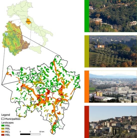
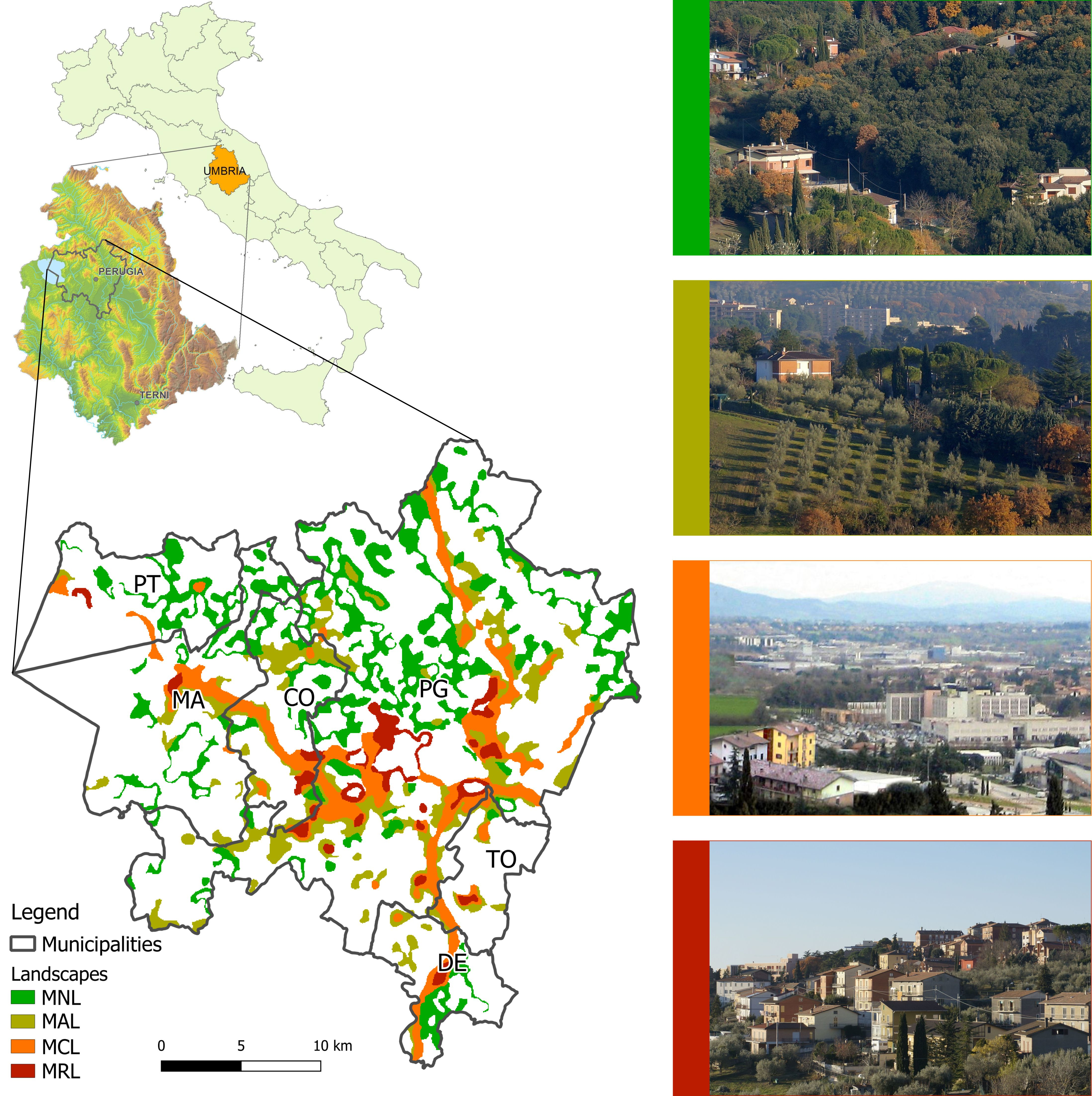
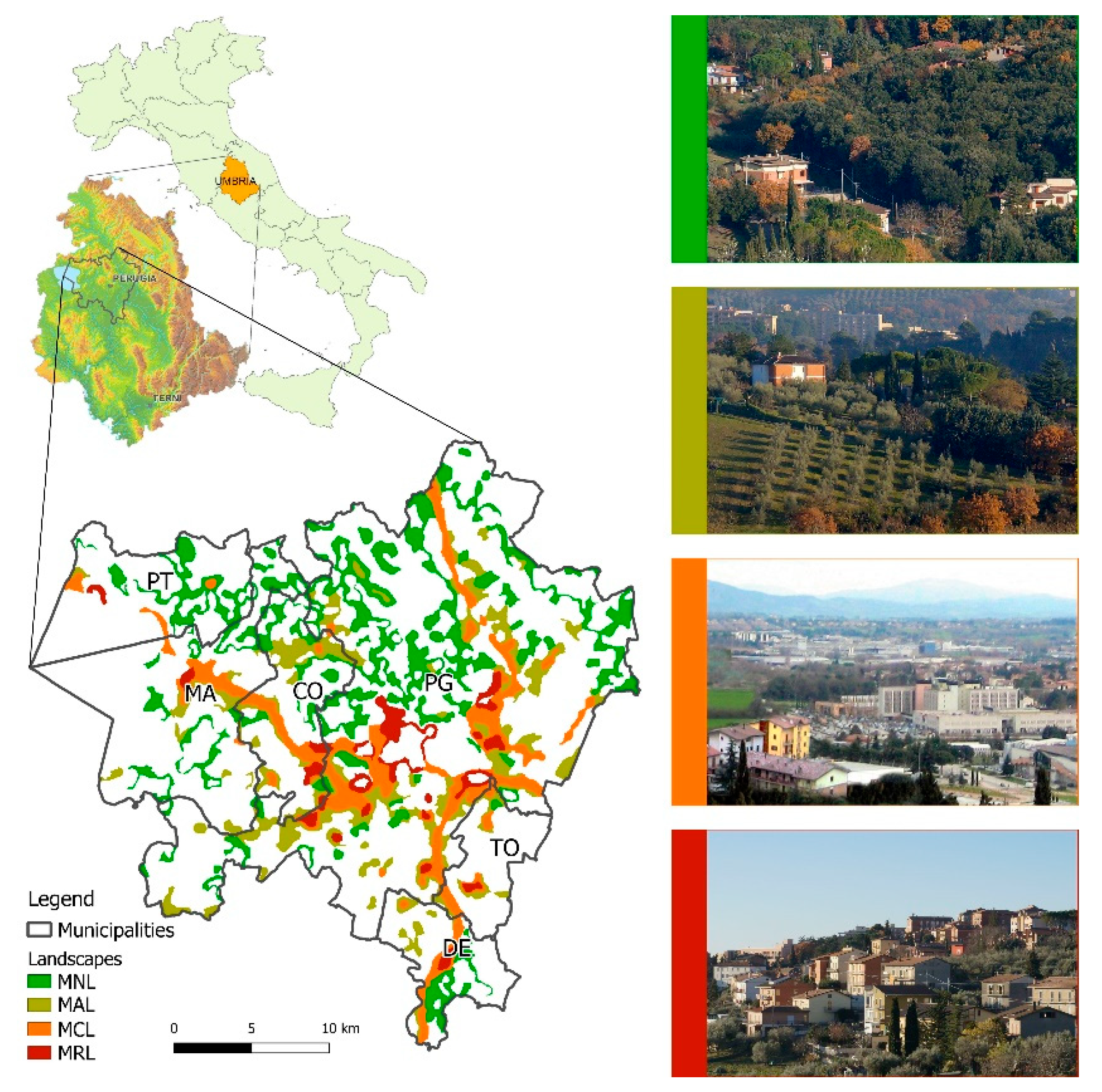
In order to understand the complex relationships established in peri-urban areas between reference urban centre, US and ES, with particular attention to the landscape, a Discrete Choice Experiment (DCE) was carried out in the transitional peri-urban areas of six municipalities located near the city of Perugia (Italy). The two main goals of this study are analysing the effect of the presence of US and ES on the demand for housing, and exploring the related implications in terms of peri-urban land use policy.

The paper is organized as follows: after a literature review in Section 2, Section 3 introduces the study area and the transitional peri-urban landscape typology, and explains the methodological steps of the DCE. In Section 4, the experiment results are reported, and an interpretation of the research findings is provided. In Section 5, the findings are discussed, and the key aspects within planning processes of the peri-urban areas are highlighted. In the last section, we draw the conclusions of our study.

2. Literature Review

The European study PLUREL, carried out between 2007 and 2010 across the 27 European states (EU27), estimated that peri-urban areas will grow four times as much as urban areas, with a comparable surface area of built-up land [7]. If confirmed, this trend could lead to doubling the current extension of peri-urban areas between 2040 and 2060. Such results have encouraged studies and investigations around the phenomenon of peri-urban areas, with a particular focus on the potential interactions between urban expansion and rural areas. For some scholars, this is a new “urban rurality” which needs a form of territorial governance able to harmonise the productive dimension with the environment and landscape [8,9,10], but also needs to find alternative development models to mitigate the impact of urbanisation and mobility [11]. Peri-urban areas are witnessing the emergence of new housing forms [12], and new processes related to food production and consumption [13,14,15]. In particular, some of the studies carried out in Italy have analysed the structural features of peri-urban areas, highlighting them as the result of a balancing act among resilience, new markets and occupational forms, innovation, and the demand for high-quality food and services [16,17,18,19].

Peri-urban processes, such as urban sprawl and transformations in the ways to use land, have evolved in different ways, generating a diverse range of landscapes, while uncontrolled processes have negatively impacted on the natural, economic and social components as a whole [20]. The lack of recognition for the role, functions and potentialities of agricultural areas is one of the reasons behind the progressive erosion of agricultural land, in favour of widespread urbanisation processes [21]. Therefore, it is crucial to plan and manage such realities not only for the sake of those who inhabit the area and their quality of life, but more generally for the sustainability of urban and rural development [22]. Settlement development models usually present greater land use, a higher reliance on individual and motorised mobility, and low chances to use public transport.

Hence the need to create careful territorial policies which limit as much as possible the negative aspects of dispersed settlements, while promoting the positive aspects related to the possible usage of ES provided by agriculture and natural areas [21,22]. Nevertheless, in order to carry out a territorial planning which maximises the benefits of living in a peri-urban area, it is necessary to understand the factors that influence housing demands and choice of housing [3,6].

Choosing a place of living depends on a number of factors, which according to economic theory essentially consist of income and individual utility function. Within their level of income, people attempt to buy a consumption bundle that maximises utility functions, and consequently their wellbeing. In terms of income, it is well known that housing costs tend to be higher in cities and lower in the outskirts, and also tend to increase according to the intrinsic features of the property (such as the surface area, type of finishing, etc.).

On the other hand, proximity to the place of work and to other services can have an undeniable effect on people’s income, because of the costs involved in accessing them. In terms of utility function, it can be noticed for instance that people tend to prefer to live close to green areas, urban as well as rural and natural [23]. Furthermore, it can be argued that people’s needs in relation to the availability of certain services tends to change throughout their lifespan, therefore in some phases of life the choice of housing is subject to the proximity to schooling and educational services, while in others the proximity to medical services is prioritised.

In light of this, it can be argued that the benefits arising from buying a house do not depend exclusively on the physical features of the property, but also on the availability of US and ES. Obviously where to buy a house also depends on the presence of some negative externalities that may be present both in urban areas (smog, noise, traffic, etc.) and in agricultural areas (smell, noise, etc.). In this work we will only consider services. ES are defined as the benefits people obtain from ecosystems [24,25]. Many ES are provided by agriculture, and can include: provisioning services such as food, fuel and fibre; supporting services such as the maintenance of soil fertility, water supply and quality; regulating services, such as mitigating the effects of greenhouse gases, carbon sequestration, pollination regulation; and cultural services, such as providing open-space, rural viewscapes, cultural heritage, recreational benefits [26].

Human needs are met by urban systems via the provision of US, which can be defined as public services and facilities at an intensity such as is historically and typically provided in cities [27]. US are provided by government bodies at local or national level, and include basic provisions, such as sanitary sewer systems, domestic water systems, fire and police protection services, and public services, such as public transport and road networks, public health, schools, recreational facilities, and so on.

The literature has dealt extensively with the evaluation of ES and US in peri-urban areas [21,28,29,30,31]. Most of the studies focus only on ES, highlighting the importance of intangible ES such as aesthetics, recreational value and cultural heritage [29], the relevance of agriculture as urban green infrastructure [30], or the significance of tangible ES with cultural services [21]. Instead, the work of Antognelli and Vizzari developed a liveability spatial assessment model (LISAM) capable of considering both the local accessibility of ES and US, and their perceived relevance as expressed by stakeholders. The authors point out how landscape liveability is strongly dependent not only on objective landscape features, but also on the subjective perception of inhabitants [31].

The demand for housing has been analysed in numerous studies that have used the hedonic pricing approach (HP) for estimating the relationship between the price of a property, its intrinsic characteristics (building type, size, state of preservation, etc.), and its locational characteristics [32,33,34,35]. The latter include ES (air quality, noise pollution, presence of private green spaces, landscape, proximity to open spaces, etc.), settlement type (central and peripheral urban areas, rural areas), US such as accessibility and proximity to the workplace and other services (school, public transportation system, etc.), and the socio-economic context (average income of residents, level of security, etc.) [36]. HP allows to estimate the marginal price for each of these characteristics, i.e., the price paid by buyers whose reservation price is close to the market price.

Despite being widely used, the HP has some analytical and operational limitations that can sometimes compromise the reliability of the results obtained [36,37].

In order to correctly estimate the marginal price of housing characteristics with HP it is necessary that the housing market be perfectly competitive, transaction costs be equal for all buyers, and all buyers on the market have the same income, the same system of preferences, and full knowledge of environmental quality [36]. Obviously, these are significant restrictions that may result in a lack of reliability of the results obtained.

Moreover, it should be noted that with HP it is not possible to identify which subjective characteristics affect the price of the properties and, therefore, the value of the amenities. In other words, with HP it is not possible to correctly identify the segmentation of the real estate market.

An alternative approach to analyse the relationship between house characteristics and environmental quality is given by Conjoint Analysis (CA) [38] and Discrete Choice Experiments (DCEs). Using these methods, it is possible to define in advance which housing characteristics are deemed appropriate to analyse. Once the attributes that are relevant for the purposes of the study have been selected, different levels are defined for each attribute. In this way it is possible to identify different types of housing (residential profiles), featuring different combinations of the characteristics (attributes) being investigated. A sample of respondents is asked to choose which residential profile they prefer out of a set of two or more alternatives. This allows to estimate part-worth utilities and willingness to pay (WTP) for each attribute level and to have information as to which factors most affect the choice of a house to be bought or rented. If the housing price is included in the attributes, it is possible to estimate the WTP for the attributes, which corresponds to the consumer surplus.

Previous studies on the housing market based on CA and DCEs are not very numerous and focus mainly on the analysis of preferences for different building types, for distance from the workplace or other services, for the settlement context, and, to a lesser extent, for the quality of residential environment [38].

The vast majority of studies have considered the intrinsic characteristics of the building (size, number of rooms, price, etc.) and travel time or distance to workplace, school, shops, etc. Other attributes considered include environmental characteristics of residential locations (air pollution, noise, flood risk) [37,39,40,41,42], presence of private green spaces [43,44,45,46], presence of public green spaces [43,44,47,48,49,50,51,52] and presence of natural or agricultural land [37,46,48]. In some cases, researchers have also considered urban, building, traffic and road, characteristics of the neighbourhood [40,43,44,48,50,51,53,54,55,56], or its social and economic characteristics (income level, safety, school quality) [39,42,48,51,56]. As for housing location, some research has included in the attributes its location in central or peripheral urban areas, or in rural areas [42,45,46,53,57,58,59].

3. Materials and Methods

3.1. Study Area

The Umbria, a small Region in central Italy, covers an area of 8464.33 km² and is inhabited by 882,015 inhabitants [60] with a relatively low urbanization and average density of 104.20 inhabitants/km².

Among the 92 municipalities, 5 are those in which most of the population is concentrated: in Perugia, Terni, Foligno, Città di Castello and Spoleto, 46% of the total population of the region resides. This research focuses on the peri-urban areas around the city of Perugia, which have been characterized in recent decades by relevant rural transformations that have led to an overall increase in urbanization and an intensification of agricultural land uses [61]. In detail, the 800 km² study area includes the city of Perugia and its surroundings consisting in five municipalities: Magione, Passignano sul Trasimeno, Corciano, Torgiano and Deruta (Figure 1).

The study area was chosen because it represents a typical Italian area in which a large proportion of the territory is characterized by various mixed landscapes where dynamic processes and instable conditions can be observed, especially in peri-urban areas at the urban fringe where there is no prevailing function (natural, agricultural, residential, commercial), but mixed land uses. From the peri-urban, environmental and landscape point of view three areas with specific territorial characteristics and four transitional landscape typologies are distinguished.

The three areas with specific territorial characteristics are: (a) flat areas at the convergence of the Tiber and Umbrian valleys rich in infrastructures, services highly polarized, and extensive residential agglomerations in the municipalities of Perugia and Corciano; (b) hilly areas characterised by the presence of Lake Trasimeno (an important tourist area) and of a sizeable built-up area, in the municipalities of Magione and Passignano; and (c) hilly and flat areas characterised by the presence of the vineyards and olive groves, Tiber river, and a large craftsmanship area, in the municipalities of Torgiano and Deruta.

At the same time within these territorial areas four peri-urban transitional landscape typologies have been identified within the TRUSTEE (Towards RUral Synergies and Trade-offs between Economic development and Ecosystem services) project, using density indicators associated with urbanisation, agriculture, and natural elements considered to be key components for the identification of landscape gradients [62]. The four peri-urban transitional landscape typologies are the following (Figure 1):

-

mostly natural landscape (MNL), characterised by a large presence of forests and field hedges;

-

mostly agricultural landscape (MAL), characterised by a large presence of olive groves, fields, and vineyards;

-

mostly residential landscape (MRL), characterised by a large presence of residential buildings and secondary roads;

-

mostly commercial landscape (MCL), characterised by a large presence of industrial and commercial buildings and main roads.

Each peri-urban transitional landscape typology is characterized by the different incidence of the main land uses: forests, field hedges, olive groves, vineyards, meadow and arable land fields, residential buildings, industrial and commercial buildings and main roads. In the map (Figure 1) the different coloured areas correspond to the four peri-urban transitional landscape typologies, while the white areas correspond to urban or rural areas where there is a prevailing function (residential or commercial, natural or agricultural). The photos are representative of the diversity of Umbrian peri-urban transitional landscape typologies.

3.2. Discrete Choice Experiments

In recent years, DCEs have become one of the most used stated preference methods to investigate environmental/landscape assets [63,64,65,66].

These models have their roots in the economic theory, and their theoretical foundations include in particular: (a) Lancaster’s theory [67]; (b) information processing models in decision making, developed in psychology [68]; and (c) random utility models [69].

Irrespective of the field of application, DCEs consist of a series of steps that together form the research design. As underlined by Hoyos (2010) [65], DCEs are designed and implemented following a cyclical process involving four steps: (1) definition of attributes and levels of provision; (2) experimental design; (3) questionnaire development; and (4) sampling strategy. Decisions made at different stages are sequentially incorporated in the final design of the Choice Model (

Table 1. The phases of the research.

STEPS:
CASE STUDY SELECTION	Identification of the study area (3 peri-urban areas)
DISCRETE CHOICE EXPERIMENT	Definition of attributes and levels of provision
	Experimental design:
	- preliminary experimental design (orthogonal design)
	- testing of the preliminary experimental design
	- priors estimation
	- final experimental design (Dp-efficient design)
	Questionnaire development
	Sampling strategy
SURVEY	Questionnaire survey
ANALISYS	Random Parameter Logit model estimation

).

3.2.1. Definition of Attributes and Levels of Provision

Attributes relating to peri-urban areas, presence of ES and US and to housing characteristics were selected (

Table 2. Attributes and levels used in the Discrete Choice Experiment design.

Attributes	Levels
Peri-urban areas	Municipalities of Perugia and Corciano; municipalities of Magione and Passignano; municipalities of Torgiano and Deruta; other area.
Distance to the workplace	Less than 15 min; between 15 and 30 min; more than 30 min.
Distance to commonly used urban services	Less than 15 min; between 15 and 30 min; more than 30 min.
Distance to green areas equipped with recreational facilities	Less than 300 m; more than 300 m.
Distance to farms with direct sales	Less than 500 m; more than 500 m.
Landscape characteristics	Mostly natural landscape; mostly agricultural landscape; mostly residential landscape; mostly commercial landscape.
Price levels	Market prices equal to 700, 900, 1200, and 1500 euros/square metres; monthly rental prices to 2.3, 2.9, 3.9, and 4.9 euros/square metre/month.

).

As for peri-urban areas we considered the three areas discussed in paragraph 2.1.

Concerning the ES, we considered the landscape as cultural service, the distance to green areas with recreational facilities as proxy of recreational benefits, and the distance to farms that sell their products directly to consumers as proxy of provisioning service. In particular, for the landscape, we utilized the four peri-urban transitional landscape typology discussed in the paragraph 2.1. As for the other two attributes, we preferred to consider the distance from home, since on the one hand their use is more occasional, and on the other it requires that the service be available within a short distance. As regards distance to green areas equipped with recreational facilities, we considered two levels: less than 300 metres and more than 300 metres. With regard to distance to farms that sell their products directly to consumers, we identified two levels: less than 500 metres and more than 500 metres.

As for US, we considered the distance to commonly used urban services (school and doctor’s surgery), as proxy of public services. Moreover, given the importance of commuting when choosing the place of residence also the distance from the workplace was considered. In both cases, we defined three levels based on travel time: less than 15 min; between 15 and 30 min; more than 30 min.

Finally, with respect to housing attributes, we considered only price. To define price levels, we referred to the database available on the website of the Italian Agency of Revenue (Agenzia delle Entrate). We used data relating to the first half of 2015 for basic/economical residential housing for the three peri-urban areas with specific territorial characteristics, which were between 919 and 1220 euro/sqm in the municipalities of Perugia and Corciano, 805 and 1200 euro/sqm in the municipalities of Magione and Passignano and 620 and 955 euro/sqm in the municipalities of Torgiano and Deruta.

We identified the following price levels: market prices equal to 700, 900, 1200, and 1500 euros/square metres, which correspond to a monthly rental prices to 2.3, 2.9, 3.9, and 4.9 euros/square metre/month. However, models were estimated using the market price per square metre, since the majority of respondents lives in owner-occupied houses.

To simplify the decision-making process, following other studies [41,48,51], no information about the intrinsic characteristics of the housing unit was given. Respondents were only told that the price referred to an immediately inhabitable ordinary dwelling, not of new construction, with an average surface area of 100 square metres located in one of the areas specified in the choice set. Although it cannot be neglected that intrinsic characteristics play a crucial role in the housing choice, excluding them allowed us to simplify the respondents’ decision-making process, by reducing the number of choice sets and the complexity of the choice tasks.

Since the study concerns peri-urban areas it can be considered that all the alternatives identified in the choice sets are plausible and realistic. In peri-urban areas it is in fact possible to reside in a predominantly agricultural or natural landscape and at the same time be close to the workplace. On the other hand, in these contexts there is no direct correlation between distance from urban services and from the workplace. Typically in the Italian peri-urban areas, there is a considerable mix of different land uses so that many productive activities and many urban services are scattered throughout the territory.

3.2.2. Experimental Design

Once the attributes and levels were defined, the experimental design was constructed. The combination of attributes and levels was necessary to define the alternatives that were included in the choice sets that were presented to respondents.

Considering the real estate market segmentation of the area under analysis, we opted for a labelled design. We used as labels the three different peri-urban areas for urban and environmental characteristics and for segmentation of the housing market (Table 1). The approach is similar to that used in other research [47]. A fourth, non-geographically defined peri-urban area was included in the experimental design. This area comprises other municipalities from which it is possible to reach Perugia to access the workplace or to use other urban services. The four areas represent the labels of the different attributes: respondents had to choose a house located in one of these four areas. This choice was made assuming that proximity to the current housing location plays an important role in dwelling choice.

A preliminary experimental design was created using an orthogonal design. The questionnaire was than tested on a sample of 50 respondents and the experimental design was optimised by means of a Dp-efficient design taking into consideration the priors obtained from the preliminary submission of the survey. The design was blocked into 2 blocks to reduce the fatigue of the respondents and to improve the reliability of the interviews. Each respondent was presented 6 choice sets with 4 choice options each. Particularly the fourth choice option, in each choice set, corresponds to the peri-urban area non-geographically defined and characterized by the commercial landscape and by all attributes at maximum levels except the price at the minimum threshold.

3.2.3. Questionnaire Development

The questionnaire is composed of an introduction, two main sections, and a final general section. The introduction presents the survey, the institutions involved in the study, and the importance of participating in the survey. It also clarifies that respondents will remain anonymous. Moreover, a box contains detailed information on the research topic, such as the composition of landscapes in transitional peri-urban areas, the characterisation of the peri-urban areas being investigated, the functions of ES and commonly used US. Information thus provided made it easier to complete the questionnaire, since not all consumers are familiar with these issues.

The second section focuses on the choice task, i.e., the preference for living in a peri-urban area over another based on the characteristics of the landscape and of the ES and US available.

Graphically, each choice option is presented using choice tasks containing four different options. For each option, the photo of the peri-urban landscape and the attributes and levels defined in the experimental design are provided (

Table 3. Example of a choice task.

	Immediately Inhabitable Ordinary Dwelling, Not of New Construction, with an Average Surface Area of 100 Square Metres
	Peri-urban areas of Municipalities of Perugia and Corciano	Peri-urban areas of Municipalities of Magione and Passignano	Peri-urban areas of Municipalities of Torgiano and Deruta	Other peri-urban areas
Distance to the workplace	Less than 15 min	Less than 15 min	More than 30 min	More than 30 min
Distance to commonly used urban services	More than 30 min	Between 15 and 30 min	Between 15 and 30 min	More than 30 min
Distance to green areas equipped with recreational facilities	More than 300 m	More than 300 m	Less than 300 m	More than 300 m
Distance to farms with direct sales	Less than 500 m	Less than 500 m	Less than 500 m	More than 500 m
Landscape characteristics
Price levels	Market prices equal to 1500 euros/square metres; monthly rental prices equal to 4.9 euros/square metre/month.	Market prices equal to 700 euros/square metres; monthly rental prices equal to 2.3 euros/square metre/month.	Market prices equal to 900 euros/square metres; monthly rental prices equal to 2.9 euros/square metre/month.	Market prices equal to 700 euros/square metres; monthly rental prices equal to 2.3 euros/square metre/month.
Specify your choice:

).

Respondents were asked to imagine that they would have to change their homes and to choose which of the four specified peri-urban areas they would move to, and in which landscape context they would have preferred to reside.

The third section includes a series of questions on the characteristics of the area in which the respondent resides and the reasons that influenced the choice of her/his current housing location.

The last section of the questionnaire collects socio-economic information about respondents (gender, age, education, place of residence, municipality of residence, employment status, household composition, and living standards).

3.2.4. Sampling

Data were collected between April and May 2016 through the administration of questionnaires to a total sample of 300 households. The collection unit considered is the common-law family, understood as a group of people living together and linked by emotional bonds, marriage, kinship, affinity, adoption, and protection.

The sampling strategy adopted for questionnaire administration is the quota sampling: starting from the population of all residents of the Umbria region, a stratified sample was identified, using as first variable the number of household members (one member; one member sharing house; two, three, four, five, or more than five members) and as second variable the housing location (urban centre, cluster of houses, and isolated houses). For both variables, reference was made to Istat Census data [70], which provide the number of resident households distinguished according to the number of members and housing location in absolute values, along with municipal detail. Crossing the two variables, we defined first the percentage of the population for each municipality and then the sample, considering that it had been established in advance to interview 50 households per municipality.

In the light of the sample size and the limited resources, two main methods were adopted to intercept respondents: the use of intermediaries and direct and random meetings with potential respondents.

The intermediaries involved were officers or managers of local institutions and organizations, such as mountain communities and local action groups, but also shopkeepers or locals. Intermediaries were tasked with introducing the interviewer to colleagues, partners, associates, and acquaintances, thus facilitating the interview. Direct meetings with potential respondents occurred during two weeks in April, in different places of the six municipalities surveyed (bars, squares, parks, cinemas, school, supermarkets). All questionnaires were administered through face-to-face interviews.

3.2.5. Model Estimation

Using data obtained from the choice experiment, a random parameter logit model (RPL) was estimated with the statistical software package NLogit6 [69,71,72,73]. RPL models have the advantage of analysing the heterogeneity of respondents’ preferences and estimating individual WTPs for each attribute. Discrete variables were dummy coded.

In order to better interpret market segmentation, the interaction of the attributes with a set of potential predictors related to socio-economic characteristics and current housing location was analysed. Significant interactions at the 90% confidence level were identified through an iterative process. In particular, the inclusion in the model of the interaction variables relating to the landscape where the interviewees reside made it possible to verify whether they prefer to reside in areas similar to those in which they currently live.

In the model, all the attributes were considered random, with the exception of price and the peri-urban areas where houses are located. For random variables, a normal distribution was assumed. Models were obtained with 1000 draws.

The following utility function was estimated:

$$U_{\left(x_i\right)}= AS{C}_1+AS{C}_2+AS{C}_3+{\displaystyle \sum }_{i=1}^n{\beta }_i{x}_i+{\displaystyle \sum }_{j=1}^s{\alpha }_{ij}{x}_i{y}_j+{\beta }_{price}Price$$

(1)

where ASC₁ is Perugia and Corciano, ASC₂ is Magione and Passignano, ASC₃ is Torgiano and Deruta, β_i is the coefficient of the ith attribute, α_ij is the coefficient of interaction between the ith attribute and the jth individual characteristic, β_price is the coefficient of price.

In this regard, it should be noted that all the studies that used DCEs to analyse the demand for housing have used linear and additive utility functions. The same happened for the researches that used the HP method. Moreover, even in the real estate appraisal, surveyors refer to additive evaluation models [74]. These valuation methods tend largely to mirror valuation procedures that are implicitly employed by home buyers.

Once the coefficients of the attributes included in the model were obtained, the average WTP for each attribute level was estimated:

$$\overline{WT{P}_i}=-\frac{{\beta }_i}{{\beta }_{price}}$$

(2)

Since interaction variables have been inserted in the model, the estimated WTP does not correspond to the average sample WTP. The following formula was used to estimate the average WTP of the sample:

$$\overline{WT{P}_{si}}=\overline{WT{P}_{gi}}+{\displaystyle \sum }\overline{WT{P}_{ji}}·P_j$$

(3)

where:

$\overline{WT{P}_{si}}=average WTP of the sample for the i^{th} attribute$

$\overline{WT{P}_{gi}}= average WTP for the i^{th} attribute estimated in the first part of the model$

$\overline{WT{P}_{ji}}= average WTP for the i^{th} attribute of the interviewees belonging to$

$the j^{th} individual characteristic$

Pj = fraction of the sample belonging to the jth individual characteristic.

For example, with reference to the data in

Table 4. Interpretative model of the factors that contribute to increasing the housing value (values in euro/square metre).

	Coeff. †		WTP	WTP C.I. (95%)
			Average	Inf.	Sup.
Random parameters (latent heterogeneity)
mostly residential landscape	1.7123	***	1542.7	979.0	2106.4
mostly agricultural landscape	2.3464	***	2113.9	1365.6	2862.2
mostly natural landscape	2.7528	***	2480.0	1536.3	3423.8
urban services within 15–30 min	0.4903	***	441.7	125.9	757.6
urban services within 15 min	0.6914	***	622.9	302.6	943.2
workplace within 15–30 min	0.6397	***	576.4	148.2	1004.5
workplace within 15 min	0.8614	***	776.1	459.7	1092.5
green area with recreational facilities within 300 metres	0.1339		120.6	−47.3	288.6
farm selling agricultural products within 500 metres	0.2926	***	263.6	46.0	481.3
Non-Random Parameters
Perugia and Corciano	0.5412	**	487.6	8.7	966.5
Magione and Passignano	0.8359	***	753.1	142.0	1364.3
Torgiano and Deruta	0.5643	**	508.4	−31.0	1047.9
Price	−0.0011	***
Heterogeneity in mean parameter: Variable
mostly residential landscape × current residential landscapes: mostly agricultural	−0.6167	**	−555.6	−1129.0	17.8
mostly residential landscape × low or low-medium standard of living	−0.9209	***	−829.7	−1428.0	−231.4
mostly residential landscape × 21–30 age group	−1.3222	***	−1191.2	−2069.0	−313.4
mostly agricultural landscape × low or low-medium standard of living	−1.1717	***	−1055.6	−1743.7	−367.6
mostly agricultural landscape × 21–30 age group	−1.3658	***	−1230.5	−2158.7	−302.2
mostly agricultural landscape × 31–40 age group	−0.6052	*	−545.3	−1128.8	38.3
mostly natural landscape × current residential landscape: mostly residential	−1.2184	***	−1097.7	−1679.5	−515.8
mostly natural landscape × low or low-medium standard of living	−0.7750	***	−698.2	−1247.1	−149.4
mostly natural landscape × 21–30 age group	−0.7887	**	−710.5	−1440.4	19.3
urban services within 15–30 min × low or low-medium standard of living	−0.5545	**	−499.6	−1008.6	9.4
urban services within 15 min × urban place of residence	0.5053	***	455.2	101.2	809.2
urban services within 15 min × low or low-medium standard of living	−0.6669	***	−600.9	−1021.3	−180.4
workplace within 15–30 min × low or low-medium standard of living	−0.5116	*	−460.9	−1001.0	79.2
workplace within 15–30 min × 21–30 age group	0.9926	**	894.3	69.8	1718.7
workplace within 15–30 min × 31–40 age group	0.9642	***	868.7	271.5	1465.8
workplace within 15 min × low or low-medium standard of living	−0.5979	***	−538.7	−940.9	−136.4
workplace within 15 min × 21–30 age group	0.7604	**	685.1	92.6	1277.5
workplace within 15 min × 31–40 age group	0.7953	***	716.5	250.4	1182.5
green area with recreational facilities within 300 metres × 21–30 age group	0.4024	*	362.5	−87.3	812.3
farm selling agriculture products within 500 metres × current residential landscape: mostly residential	−0.4743	***	−427.3	−725.9	−128.7
Standard deviations of random parameters distributions
mostly residential landscape	0.8435	***
mostly agricultural landscape	1.6051	***
mostly natural landscape	1.2814	***
urban services within 15–30 min	0.4655
urban services within 15 min	0.5731	***
workplace within 15–30 min	0.6988	***
workplace within 15 min	0.8132	***
green area with recreational facilities within 300 metres	0.1457
farm selling agricultural products within 500 metres	0.2524

^† Significance levels: *** significant at the 99% level; ** significant at the 95% level; * significant at the 90%. N. Observations = 1800 Loglikelihood = −2495.32 McFadden pseudo R-squared = 0.2317 Halton draws = 1000.

(reported in the results section) in the case of the “mostly residential landscape” attribute the sample mean WTP was calculated as follows:

$$\begin{array}{ll}\overline{WT{P}_{si}}=\overline{WT{P}_{gi}}& + \overline{WT{P}_1}·P_1+ \overline{WT{P}_2}·P_2+\overline{WT{P}_3}·P_3\\ & =1542.7-555.6·0.187-829.7·0.303-1191.2·0.120\\ & =1044.4 euros per square metre\end{array}$$

where:

$WT{P}_{si}=average WTP of the sample$

$WT{P}_{gi}=average WTP without interaction terms$

$WT{P}_1=average WTP of people living in mostly agricultural landscape$

$WT{P}_2=average WTP low or low-medium standard of living people$

$WT{P}_3=average WTP of 21-30 age group$

P1 = fraction of interviewees living in mostly agricultural landscape

P2 = fraction of interviewees with low-medium standard of living people

P3 = fraction of interviewees belonging to 21–30 age group

To correctly interpret the results, it should be specified that $\overline{WT{P}_i}$ represents the average WTP of respondents and corresponds to the average consumers’ surplus of the interviewees. This amount cannot be compared with the market price, which corresponds to the WTP of marginal consumers, i.e., buyers whose reservation price is close to the market price. It is therefore not surprising that the $\overline{WT{P}_i}$ may appear remarkably high compared to the market price of a property. Moreover, since the coefficients of demand functions estimated using HP correspond to the marginal price of the dwellings’ characteristics, i.e., the WTP of marginal consumers, the estimates obtained with DCE cannot be compared with those obtained with HP.

Finally, it must be remembered that the estimated WTP is always a marginal value since it corresponds to the difference between the value of the benefits obtainable from having a home in the situation constituted by the status quo and those deriving from residing in each of the other alternatives identified in the experimental design. However, these data permit to calculate the variation of the WTP with reference to the different scenarios present in the DCE.

4. Results

4.1. Characteristics of Respondents

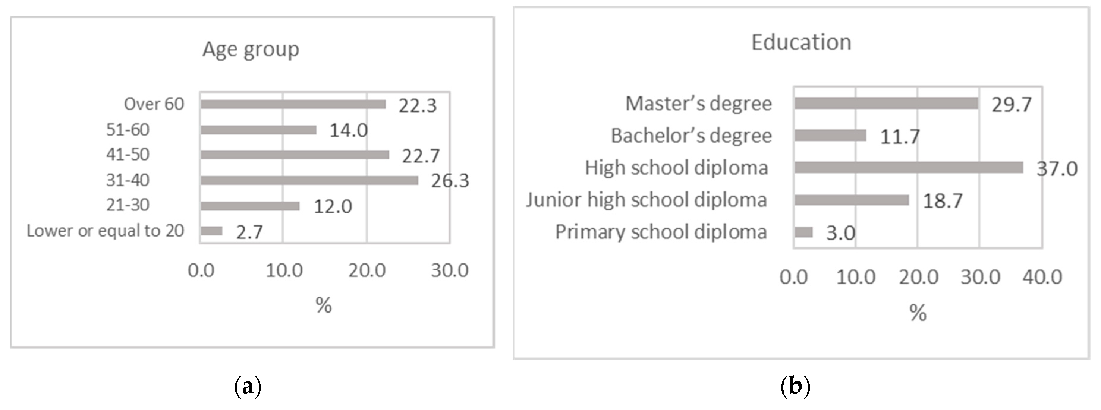
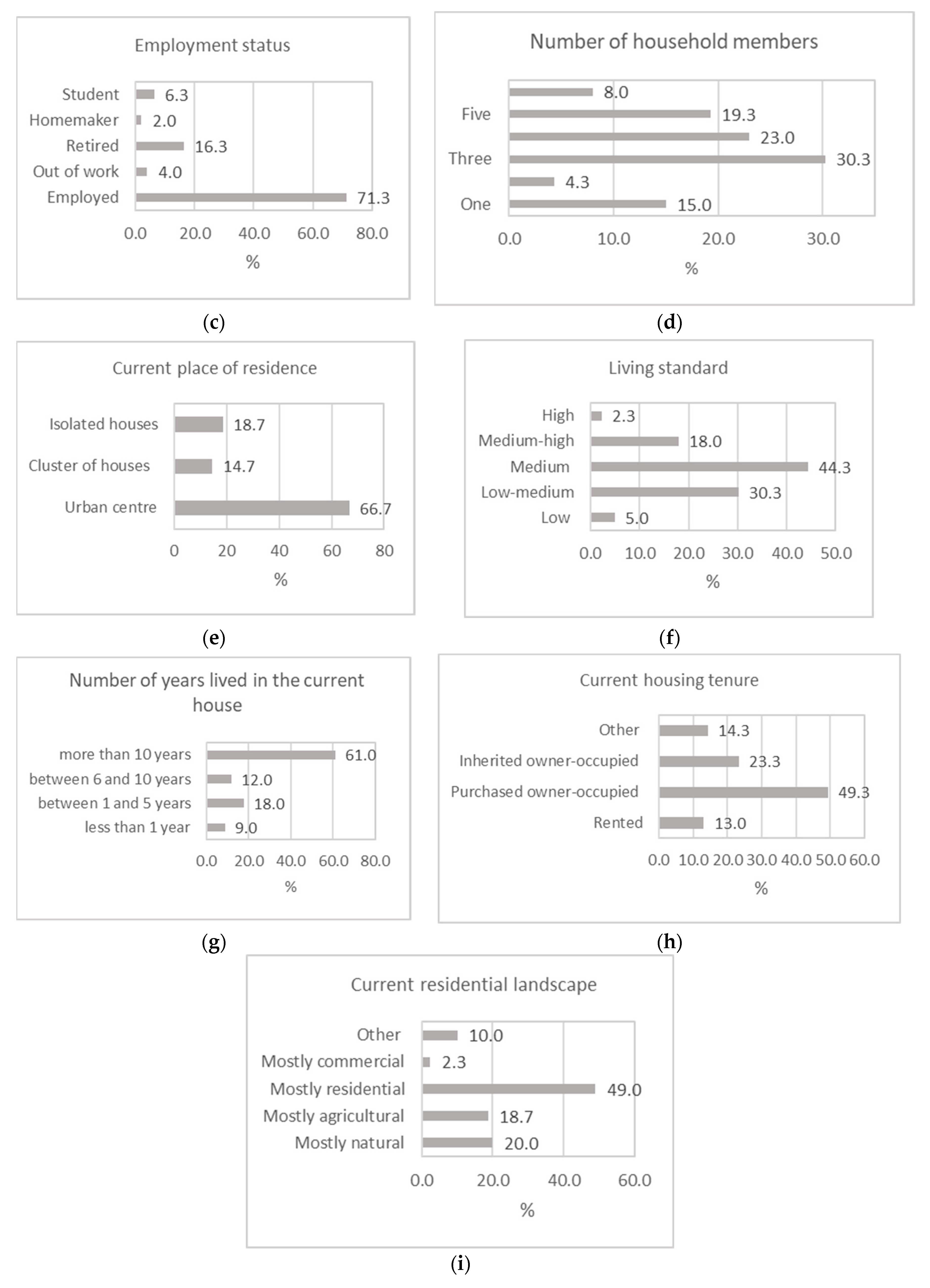
The majority of respondents were women (56%) and the most represented age group is the one ranging from 31 to 50 years (49%) (Figure 2). A total of 21.7% of respondents obtained less than a high school diploma, while 30% of them held a master’s degree or even a higher degree. As regards employment status, 71.3% of those surveyed were employed, while 16.3% of them were retired. Only 4% of the sample was out of work and 2% were homemakers. Percentages for the composition of the common-law family correspond to those of the stratified sample, thus reflecting the breakdown of the population with respect to the reference municipality: 50.3% of households were composed of three or four members and 15% of them were one-person households. Most respondents (74.6%) considered their standard of living to be medium or low-medium, whereas 20.3% of them considered it medium-high or high.

Most respondents resided in urban areas (66.7%) (Figure 2). A total of 49% of those surveyed regarded the landscape in which they live as a residential landscape, while for 38.7% of them it was mostly natural or agricultural. A total of 61% of the sample had lived in the current house for more than 10 years, whereas 27% of the sample for less than five years. Therefore, their housing choice was quite recent. It should be noted that a significant percentage of the sample (23%) lived in an inherited house. Thus, their housing choice was conditioned by this opportunity. Quite an important percentage of the sample purchased the own-occupied house, while rented houses account for 13% of the sample.

A total of 43% of respondents stated that they know the housing market, although only 20% of them were willing to change their house.

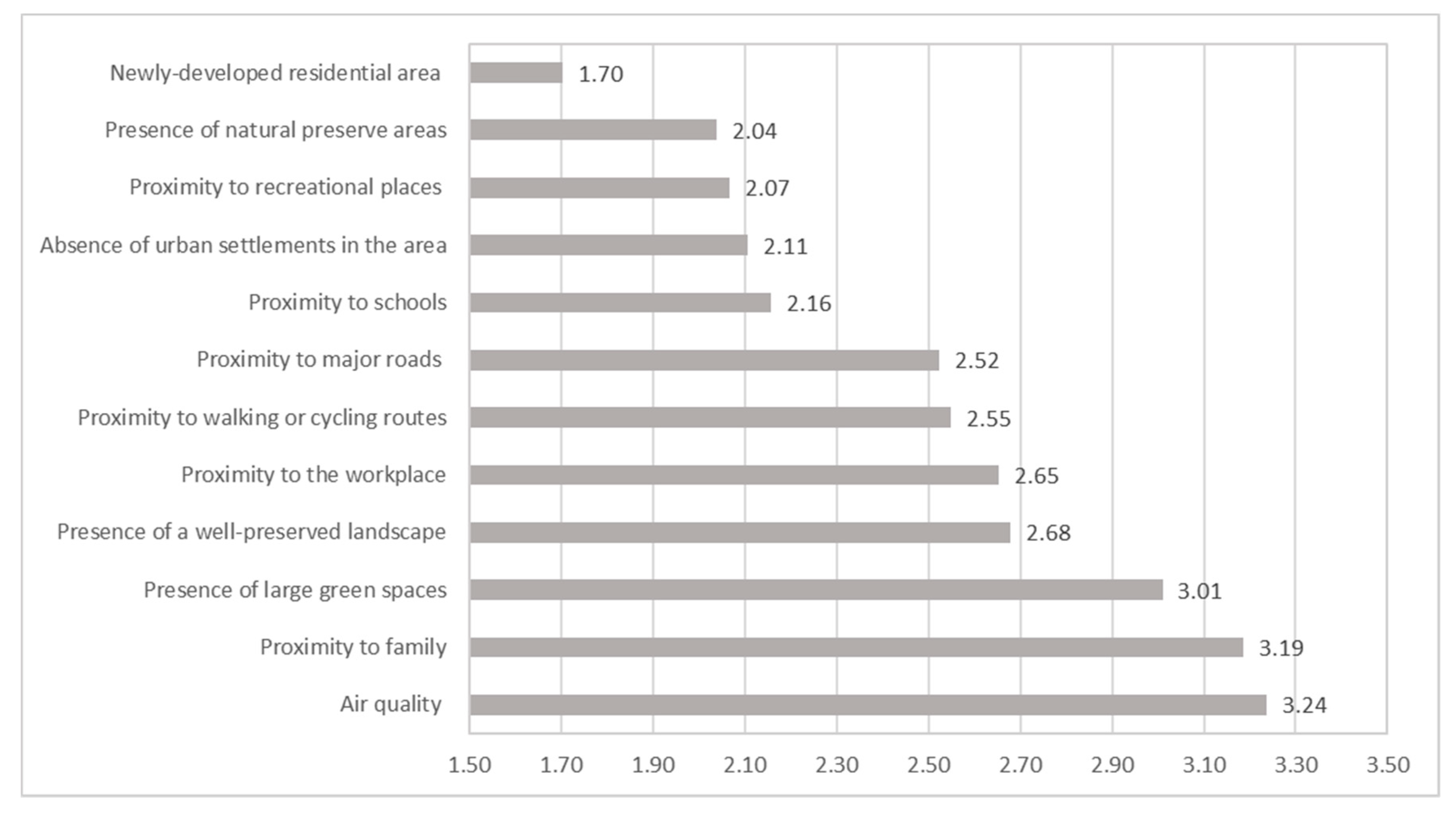
According to the interviewee’s statements, the criteria that influenced the choice of the current place of residence are mainly air quality, proximity to family, and the presence of large green spaces (Figure 3). On the other hand, the variables that played a minor role and had less influence are proximity to recreational places (cinemas, theatres, restaurants, discos, etc.) and the presence of natural preserve areas and newly-developed buildings.

4.2. The Value of Ecosystem Services and Urban Services

Table 4 illustrates the estimated model and the average WTP for each of the attributes considered in the choice experiment that represents the average WTP for one square metre of a dwelling. As observed, only significant interaction variables were included in the model with at least 90% probability: low or low-medium standards of living, the prevailing landscape in the current place of residence (mostly residential or mostly agricultural landscape), and age (21–30 and 31–40 ages groups).

It is interesting to note that the other socio-economic characteristics (for instance, education level and employment status), as well as the stated housing market knowledge and the search for a house, to be bought or rented, do not seem to influence significantly the interviewees’ choices.

The model has a good interpretative capacity of the phenomenon under analysis (McFadden pseudo R-squared = 0.231). All the coefficients are statistically significant at the 95% confidence level. Exceptions to this are represented by the presence of open green spaces equipped for leisure time within 300 metres (p = 0.1182), the interaction between mostly agricultural landscape and the 31–40 age group (p = 0.0501), the interaction between workplace within a 15–30 min distance and a low or low-medium standard of living (p = 0.0609), and the interaction between the presence of open green spaces equipped for leisure time within 300 metres and the 21–30 age group (p = 0.0978) (Table 4).

Six out of nine attributes exhibit a statistically significant degree of heterogeneity. In particular, preferences seem to be more homogeneous for attributes that have a lower average WTP (farm selling agricultural products within 500 metres, open green spaces within 300 metres, services within 15–30 min).

To improve the readability of the data,

Table 5. WTP of interviewees belonging to different individual characteristics group and average willingness to pay estimation (euro/square metre).

	Base Model	Place of Residence		Standard of Living	Age		Interviewees Average WTP
		Mostly Agricultural	Mostly Residential	Low or Low-Medium	from 21 to 30	from 31 to 40
mostly residential landscape	1542.7	−555.6		−829.7	−1191.2		1044.4
mostly agricultural landscape	2113.9			−1055.6	−1230.5	−545.3	1503.0
mostly natural landscape	2480.0		−1097.7	−698.2	−710.5		1645.4
urban services within 15–30 min	441.7			−499.6			290.4
urban services within 15 min	622.9		455.2	−600.9			663.9
workplace within 15–30 min	576.4			−460.9	894.3	868.7	772.5
workplace within 15 min	776.1			−538.7	685.1	716.5	883.5
green area with recreational facilities within 300 metres	120.6				362.5		164.2
farm selling agricultural products within 500 metres	263.6		−427.3				54.3

shows the WTP relating to the individual characteristics inserted as interaction terms in the model reported in Table 4.

As regards proximity to the workplace or US, the results obtained are consistent with those reported in international literature. It can be seen that the WTP is inversely proportional to the distance from the workplace and the main commonly used US (schools, shops, doctor’s surgery, public transportation system).

With reference to the workplace, respondents with a medium or medium-high standard of living and over the age of 40 are willing to pay 776 euros/square metre more for a house located within 15 min of the workplace than for a house located more than 30 min from the workplace. This price decreases to 576 euros/square metre if the travel time to workplace is between 15 and 30 min by car. The WTP for a house close to workplaces decreases for respondents with low-medium or medium standards of living and it increases for younger respondents (Table 5). The higher WTP of younger people is essentially due to the fact that, since they have a longer working life ahead, the accumulation at present of the value of the time spent to reach the workplace is higher than that of older people so they are willing to pay more to buy a house closed to the workplace since in this way they have the possibility to save more money than older people.

The lower WTP of those who have a low or low-medium standard of living may be explained essentially by the lower opportunity cost of travel time, which is to be related to the average income of the respondents or of the household members.

The WTP to gain access to US such as school, doctor’s surgery, etc. is slightly lower than the WTP to access the workplace. It ranges from 622.9 euros/square metre to 441.7 euros/square metre depending on whether they can be reached within 15 min or between 15 and 30 min. It is interesting to note that in this case the age of respondents is not statistically significantly correlated with accessibility to services. This result is consistent with the results obtained with respect to the time spent to reach the workplace. The use of many services characterises the whole life of respondents and although it is true that as people grow older some of these services assume less importance (for example, proximity to school), others tend to be more and more relevant (for example, accessibility to health services).

Furthermore, in the case of access to services, the WTP decreases significantly for those who have a medium or low-medium standard of living (−600.9 euros/square metre). On the other hand, it increases for those who currently reside in a mostly residential context (+455.2 euros/square metre). This is not surprising if we consider that urban dwellers are used to easily accessing all the services offered by the city and are therefore willing to pay more as not to lose them.

Proximity to green areas with recreational facilities is not statistically significant (p = 0.118) and it corresponds to a very low figure (120.6 euros/square metre).

The opportunity to buy agricultural products directly from the producer seems to be quite appreciated by respondents (263.6 euros/square metre), although among urban dwellers it seems to have a mostly negative effect, since it considerably reduces the WTP (−427.3 euros/square metre).

Landscape quality is certainly the factor that most affected the WTP of respondents. Passing from mostly residential landscapes to mostly agricultural landscapes, the WTP increases by 571.2 euros/square metre, while passing from mostly residential landscapes to mostly natural landscapes, the WTP increases by 937.4 euros/square metre. The presence of natural and agricultural landscapes seems to be able to significantly increase the housing value (obviously, it should be noted that average WTPs cannot be compared with market prices of houses, since they represent the average consumers’ surplus, namely they provide a measure of the social benefits that they would enjoy if they were to live in more pleasant agricultural landscapes). Furthermore, in this case the WTP decreases significantly among respondents with a lower standard of living. This phenomenon concerns mainly mostly agricultural landscapes (−1055.6 euros/square metre), but it also involves residential (−829.7 euros/square metre) and natural (−698.2 euros/square metre) landscapes. Besides this, it can be noted that, in general, younger people have a lower WTP for all the landscapes considered.

It is also interesting to note that the current place of residence influences the benefits related to residing in different landscapes. Therefore, those who currently live in agricultural areas have a WTP lower than 555.6 euros/square metre for houses located in residential landscapes. Conversely, those who currently live in a residential landscape have a WTP lower than 1097.7 euros/square metre for houses located in mostly natural landscapes.

Finally, it should be emphasized that the municipality where the house is located also has a significant effect on the WTP of the interviewees. Respondents reported a higher WTP to reside in the peri-urban area of Magione and Passignano (753 euros/square metre) and Torgiano and Deruta (508 euros/square metre) compared to Perugia and Corciano (487 euros/square metre). Probably this is due to the fact that near Magione and Passignano there is the presence of Lake Trasimeno which constitutes an important naturalistic area and provides significant opportunities for recreational activities. On the other hand, in the peri-urban area of Perugia there is a very high traffic and the air is most polluted.

The average WTP for each of the attributes of the whole sample was calculated using formula (3) (Table 5).

It can be observed that the WTP is much higher for the mostly natural landscape (WTP = 1645 euros/square metre) and mostly agricultural landscapes (1503 euros/square metre) than for urban ones. (1645 euros/square metre). In general, the proximity of homes to services and the workplace is also very important, while proximity to urban green space and farms selling agricultural products produces significantly lower benefits. It can be noted that the WTP for a home that allows people to reach their workplace in less than 15 min is 880 euros/square metre higher than that for a home from which people can reach it in more than half an hour. Similarly, the WTP for a home that has access to the most common urban services in less than 15 min is 663 euros/square metre higher than if US can only be reached in more than half an hour.

5. Discussion

The study has shown that the availability of some ES can have a significant influence on the housing choice. The benefits of living in areas with mostly agricultural or natural landscapes are the main factor affecting the WTP of some segments of the housing demand in the study area. This result is consistent with the findings of other research. As for agricultural areas, Bullock, Scott, and Gkartzios (2011) [46] have highlighted that views of countryside and fields contribute to increasing the price of the houses. Earnhart (2001) [37] has shown that proximity to wetlands and forests increases the housing value, while according to Roe, Irwin, and Morrow-Jones (2004) [48] the preservation of 10% of the existing open space within one mile of the house can increase its value from 3% to 6%.

The high WTP of respondents for a house located in mostly natural and, to a lesser extent, mostly agricultural landscapes are to be related to the multiple benefits that these areas can bring to residents in peri-urban areas. Literature has shown that natural or semi-natural landscapes can influence people’s well-being, by improving their emotional, physical, and cognitive state [75,76]. The presence of natural areas can encourage physical activity, improve air quality, reduce mental stress, and promote social cohesion.

Contrary to expectations and in contrast to previous research [43,47,48,50], the influence of proximity to open spaces equipped with recreational facilities on the WTP of respondents was not statistically significant (p = 0.13). In this respect, it is worth noting that some studies have shown that the effect of the presence of public parks and green areas with recreational facilities can be rather limited and tends to diminish rapidly as the distance increases [77,78,79]. However, it should be noted that among respondents aged 21 to 30 the coefficient of open green spaces within 300 metres is slightly significant (p = 0.097) and the WTP is considerably high.

One unanticipated finding, which cannot be found in previous research, is the importance of the accessibility to farms that sell their products directly to consumers. However, this is important only for those who do not currently reside in urban centres. In this regard, it is possible to suppose that people living outside the urban centres are used to buy farms products and want to continue to do so in the future since there are many benefits associated with the possibility of purchasing agricultural products directly on the farm. First, this allows you to consume products that preserve better their organoleptic properties because of the reduction of the time elapsing between harvesting and consumption. Second, this allows consumers to directly get to know the environment in which the products consumed are made, as well as to control producer’s reliability and to become familiar with the production techniques that are used.

In contrast to previous research, this study has also shown that the corresponding WTP for the different types of ES are highly fragmented. The WTP for living in agricultural or natural landscapes is much lower for those respondents who stated a low or low-medium standard of living, that is, about 35% of the sample. Similarly, respondents aged under 30, who account for 40% of all respondents, have a WTP significantly lower than the average of the sample, especially with respect to the importance given to mostly agricultural landscapes. This may be partly due to the greater importance they attach to proximity to the workplace, which seems to be the main factor underlying their housing choices. The lower WTP of respondents aged 21 to 30 for mostly natural landscapes can be explained in part by the higher demand for green spaces equipped for recreational activities in this segment of demand.

These findings can be useful to adopt territorial and environmental policies aimed at satisfying the needs of local population. First, in agreement with Ives and Kendal [80], a broad range of peri-urban landscape values should be considered when making land use decisions. Second, integrated policies are needed for peri-urban areas to guarantee access to US and, at the same time, the benefits of natural and agricultural environments. The challenge will be to integrate The New Urban Agenda for sustainable development [81] with the Common Agricultural Policy after 2020 within the objectives of the Sustainable Development Goals (Agenda 2030). Housing and urban mobility policies capable of preserving agriculture and green infrastructure, during urban expansion, are needed. But this can only be reached by understanding economic, social, and ecological roles of agricultural and natural systems, within the urban system.

6. Conclusions

This paper contributes to the literature in the field of ES and US and the preference of housing location in peri-urban areas by looking at a chosen set of criteria. This study agrees with previous findings related to the influence of agricultural or natural landscapes in the WTP and, at the same time, it shows that the WTP for different types of ES is highly fragmented. These findings underline that WTP is related both to peri-urban landscape typologies and some city-dwellers characteristics, such as age and standard of living. At the same time, the paper provides hypotheses to explain those results, and further research and investigations are needed so that these can be tested.

First, looking at the possible limits of the research, the effect of the current place of residence on choice of a house should be taken more into consideration, as well as the choice of the comparative situation which should really be the same for all respondents and not just from a theoretical point of view. A second aspect that deserves further investigation is the possibility for the respondents to buy a plot and construct their own house according to own wishes.

Despite the possible limits of the study, based on our findings, we suggest the following clear policy recommendations. First, it is worth noticing the importance of promoting the preservation of natural and agricultural landscapes in peri-urban areas. As mentioned above, these partly replace public green spaces equipped with recreational facilities, at least for certain groups of people. Hence, their improvement could reduce the costs associated with the creation and maintenance of public green areas. However, in this respect, it is important to implement measures aimed at fostering access also to private green spaces that are close to peri-urban areas. Moreover, the presence of farms that sell their products directly to consumers should be appropriately promoted. The development of alternative food networks (AFNs) could find their natural space for growth in these peri-urban areas, promoting the balance between the resilience of peri-urban agriculture, innovation in the food supply chain and demand for high-quality food. Acting in this direction not only would encourage direct contact between consumers and producers (thus reducing time and costs associated with marketing food products), but it would also allow the preservation of open spaces and agricultural landscapes.

Finally, in analysing both the housing demand and the availability of ES and US in the study area, the DCE method provides crucial insights. Being based on respondents’ statements, and not on the analysis of their actual behaviour, such method may lead to estimates that may not always be reliable [82]; nevertheless, it can still be a useful tool to understand the relative importance of the environmental and landscape characteristics in influencing housing choices. It can also be particularly useful to identify possible market segments that would not be otherwise identified through other approaches.