Article

Assessment Method and Scale of Observation Influence Ecosystem Service Bundles

by
Santiago Madrigal-Martínez
1,2,* and
José Luis Miralles i García
1
1
Department of Urban Planning, Universitat Politècnica de València, Camino de Vera s/n, 46022 Valencia, Spain
2
Postgraduate School, Universidad Ricardo Palma, Av. Benavides 5440, Santiago de Surco, Lima, Peru
*
Author to whom correspondence should be addressed.
Land 2020, 9(10), 392; https://doi.org/10.3390/land9100392
Submission received: 18 September 2020 / Revised: 14 October 2020 / Accepted: 14 October 2020 / Published: 16 October 2020

Abstract

:
The understanding of relationships between ecosystem services and the appropriate spatial scales for their analysis and characterization represent opportunities for sustainable land management. Bundles have appeared as an integrated method to assess and visualize consistent associations among multiple ecosystem services. Most of the bundle assessments focused on a static framework at a specific spatial scale. Here, we addressed the effects of applying two cluster analyses (static and dynamic) for assessing bundles of ecosystem services across four different scales of observation (two administrative boundaries and two sizes of grids) over 13 years (from 2000 to 2013). We used the ecosystem services matrix to model and map the potential supply of seven ecosystem services in a case study system in the central high-Andean Puna of Peru. We developed a sensitivity analysis to test the robustness of the matrix. The differences between the configuration, spatial patterns, and historical trajectories of bundles were measured and compared. We focused on two hypotheses: first, bundles of ecosystem services are mainly affected by the method applied for assessing them; second, these bundles are influenced by the scale of observation over time. For the first hypothesis, the results suggested that the selection of a method for assessing bundles have inferences on the interactions with land-use change. The diverse implications to management on ecosystem services support that static and dynamic assessments can be complementary to obtain better contributions for decision-making. For the second hypothesis, our study showed that municipality and grid-scales kept similar sensitivity in capturing the aspects of ecosystem service bundles. Then, in favorable research conditions, we recommend the combination of a municipal and a fine-grid scale to assure robustness and successfully land-use planning processes.

Graphical Abstract

1. Introduction

The ecosystem services (hereafter ES) concept—the benefits obtained from nature for human well-being [1]—has become an integrated framework in sustainability science [2]. The ES framework facilitates ecosystem conservation opportunities [3] and affords innovative and valuable data to help decision-making [4]. In that sense, ES research is a significant and rising field of research [3], gathering studies around the world that are largely focused on the assessment and the management of the state of ES [3,5]. Relationships between ES are an issue that has received increasing interest in the literature [6,7,8,9,10]. These review studies addressed the importance of the analysis of relationships between ES.
ES relationships vary over time [11,12,13,14] and depending on the scale of observation. For example, a situation of mutual enhancement among a pair of ES at the county level could become in an increase in one service at the expense of the other at grid scale [15]; also, a set of ES characterized by a multifunctional pattern of supply at municipality level can derive in a set of ES dominated by the provision of few services at the patch scale [16]. These relationships, namely synergies and trade-offs [17,18] and bundles [19], can also differ on the method for assessing them. For example, the correlation analysis between two ES for a given time can detect a trade-off, while the same analysis between the differences in ES supply at two times detect a synergy [20].
However, most of the assessments focused on a simple (static) method for estimating ES on a specific spatial scale [21], and few studies integrated historical analysis (e.g., in [11,12,22,23]). Thus, only a limited number of studies identified the effects of different spatial scales on ES (e.g., in [16,24,25,26,27,28]), but using a snapshot approach (ES assessment at a single point in time). Thus, improvement of the characterization of spatiotemporal co-occurrences of ES, applying different assessment methods at different scales of observation, can contribute to reinforcing efficient management strategies that seek to achieve win–win solutions [9].
Among the common methods for assessing ES relationships, there is correlation analysis, and cluster analysis [10,29]. Correlation analysis is mostly applied to measure the degree of statistical dependency between a pair of ES for a given time in order to classify their relationship as trade-off or synergy [6,30]. Cluster analysis is one of the main statistical methods utilized for the estimation of bundles of ES for a given time [8,31]. Bundles have appeared as an integrated method to assess and visualize consistent associations among multiple ES derived from the different land use and land cover types [19]. Different authors explored how the ES bundle concept contributes to including ES models into land-use planning [32,33], to clarify the impacts of land-change dynamics on ES [12], to identify priority areas for ES management [34], to distinguish social preferences toward ES [35] or to investigate ES bundles for analyzing trade-offs [19,36,37,38]. Despite these increasing efforts, there are still two main current methodological limitations. One related to the deficiency of standardized applicable assessment methods of ES [21,39], and other to the understanding of how the relationships between services changes at multiple time steps, and which might be the appropriate spatial scales in empirical or modeling ES research [40,41]. The different methods applied for the assessment of relationships between ES can lead to different interpretations [6,20,42,43]. Added to this, the use of a single scale of observation on ES assessments can lead to the avoidance of relationships between ES and ignore differences in spatial patterns between them when changing analysis scales [15,16,28].
In this study, we aim at examining the differences in applying two frameworks (static and dynamic) for the assessment of bundles of ES at four scales of observation over time, to provide new insights for better management of ES. To achieve these objectives, we addressed two hypotheses: first, bundles of ES are mainly affected by the method applied for assessing them; second, these bundles are influenced by the scale of observation over time. We develop the research in a case study system in the central high-Andean Puna of Peru [12,44]—this section of the moist Puna region shows a distinctive socio-ecological significance. The moist Puna (Peru and Bolivia) has been occupied, and its resources profited during several millennia by Andean civilizations [45,46]. This mountain environment, where its main social ecosystems consist of natural grassland, shrubland, and agricultural areas, can provide multiple ES [47].
We performed the analyses using the ES matrix. It is a successful method, appropriated worldwide [48,49]. It consists of an evaluation of ES using land use/land cover maps and expert estimation that is useful for spatial comparisons between regions [50]. The expert knowledge serves as a surrogate of empirical observations in many scientific studies [51]. Roche and Campagne [52] have proved that expert knowledge through the matrix approach can be as valid as the use of empirical data or biophysical indicators for ecosystem service assessment. Moreover, the matrix provides a high performance to integrate all types of information, and when the source data are scarce, this method can be the best accessible alternative for ES estimations [53], helping cross-study comparisons and decision-makers to solve the necessity of more ES appraisals for land management.
In our work, we studied the effects of applying two cluster analyses for assessing bundles of ES over time (years 2000, 2009, and 2013). We computed one (static) analysis with ES values and one (dynamic) with the amounts of changes in ES values at two times (ΔES, for short). We performed the assessments across four scales of observation: two administrative levels (provincial and municipal) and two grid resolutions (3 × 3 km and 0.25 × 0.25 km). To determine the differences between the results of each method, we measured and compared the configuration, spatial patterns, and historical trajectories of ES bundles. Additionally, a sensitivity analysis that simulated a scenario with changes in the scores of ES potential supply over time tested the inconsistencies of the ES matrix on the findings.

2. Materials and Methods
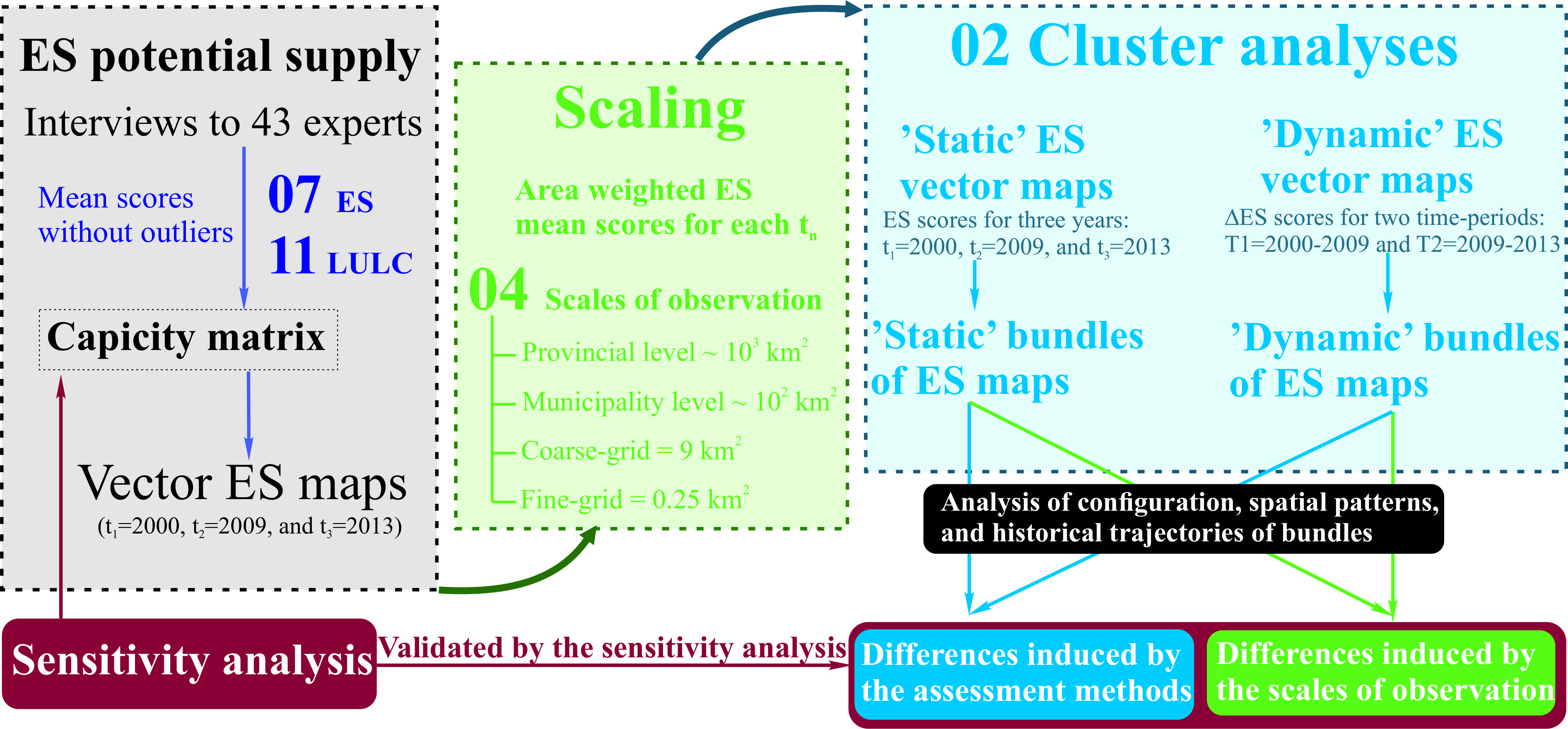
2.1. Study Site

The selected area is a section (12 provinces, 27,612 km2) of a larger study site (24 provinces, 64,025 km2) of previous studies [12,44] in the central high-Andean moist Puna (administrative departments of Junin, Huancavelica, and Ayacucho) (Figure 1). During the study period, these chosen provinces are characterized by high land-use change intensity [44], mainly due to farming expansion, agricultural de-intensification and deforestation [12]. Additionally, this study site has a high population density in the moist Puna, about 44 inhab./km2 (2013), with the strongest urban development in the metropolitan areas of the two major cities, Huancayo and Ayacucho [54].
This landscape is dominated by an expansion of livestock breeding in the upper lands and an increase in farming in the fertile lowlands. This is typical of many mountain agroecosystems across the world. Most of this territory is embedded within the Mantaro river basin, including ecosystem services associated with agricultural practices (crops and livestock provision, regulation of soil erosion and maintenance of soil quality), hydrological cycle (water purification and water flow regulation) and climate regulation. However, the main land use/land cover in the study area consists of natural grasslands (59%), shrublands (16%), and agricultural lands (15%) by 2013 (Table S1, Supplementary Materials). The diverse combination of them formed three groups of landscapes. A group of provinces (Acobamba, Huamanga, Huanta, and Vilcas Huaman) show a uniform distribution of the main land use/land cover (hereafter LULC) units (31%, 34%, and 31%, respectively). The second pattern, described by two provinces (Jauja and Chupaca), displays a territory mainly dominated by two LULC units (72% of natural grassland and 19% of farming areas). The third group of provinces (Angaraes, Cangallo, Concepcion, Huancavelica, Huancayo, and Huaytara) discloses a landscape characterized by low farming development (14%), the highest high-Andean wetland coverage (3%) and high pasture extent (63%).

2.2. Land Use/Land Cover Data Sources

The study area is covered by 11 LULC types (Figure 1). These categories, included in the Peruvian standardized nomenclature of the Corine Land Cover (CLC), were derived from three-time data sources: the map of high-Andean ecosystems in 2000 [45], the official flora cover map from 2009 [55], and the official flora cover map from 2013 [56]. According to the official sources, the maps were submitted to a verification and field survey procedure for improving the accuracy of the land use/land cover classification. However, the different geographical scales made necessary a generalization of the land use/land cover classes. Table S2 (see Supplementary Materials) shows the harmonization of the three-time step features to obtain a common legend of eleven LULC units. Moreover, the description of satellite images, mapping scale, minimum mapping area, and type of data of the three source maps are specified in Table S3 (see Supplementary Materials).

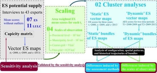
2.3. Ecosystem Services Potential Supply

The study is based on the capacity matrix that was done specifically for assessing the ES in the study area, developed by Madrigal-Martínez and Miralles i García [12] (subsequently referred to as the High-Andean Study). The assessment obtained the potential supply of 7 site-specific ES identified by the Common International Classification of Ecosystem Services [57]—two regulating services related to mediation of flows (regulation of soil erosion and water flow regulation); one ES related to filtration, sequestration, storage or accumulation by ecosystems (water purification); two services linked to the maintenance of physical, chemical, biological conditions (soil quality and global climate regulation) and, finally, two provisioning services related to nutrition (crops and reared animals).
To develop the ES matrix, the High-Andean Study consulted 43 experts to rank the ES potential supply associated with a specific LULC on a relative spatial scale, ranging from 0 (no relevant ES potential supply) up to 5 (very high ES potential supply). The experts were carefully selected to increase confidence according to their specific skills on ES and the moist Puna ecosystems. Additionally, the survey was thoroughly described individually, and they scored only the LULC/ES pairs that were sure in their judgments. Each response was collected and deprived of outliers using the interquartile range method. Then, a final score was computed using the mean. Furthermore, the potential supply of the LULC in provisioning services was achieved from official model results included in land planning instruments of the administrative departments under study. Table S4 (see Supplementary Materials) provides the maximum capacity of the eleven LULC categories to supply the seven ES. The ecosystem services were set as constant values assuming that land units are in good condition during the study period.

2.4. Scaling Method

The ES and ΔES maps were derived from the matrix model and upscaled to four spatial scales: two administrative divisions (provincial and municipal) and two grids (coarse and fine). The four spatial scales were selected for their particular importance in spatial planning and ecosystem services mapping. The provincial level (~103 km2) has a central role in the Peruvian planning system binding national and departmental directives with local interventions (Organic Law of Municipalities No. 27,972). The municipal level (~102 km2) is where land-use management in urban areas and the countryside are made. Coarse-grid resolution (9 km2) was chosen because it explores patterns of ecosystem services and approximates a locality. A fine-grid (0.25 km2) was included because it is where individual land-use management and land-cover changes occur. This spatial scale was decided as the finest because the study maps are based on a geographical scale of 1:100 000, and following the Corine Land Cover approach and the official flora cover map from 2009 [55], this spatial resolution corresponds to the minimum mapping area. Both grid resolutions are important for planning green infrastructure to support human well-being.
The administrative areas were calculated using boundaries from the Peruvian National Institute of Informatics and Statistics. The 12 provincial units range from 750 to 6075 km2 (with an average of 2301 km2), whereas the 175 municipality units vary from 5 to 2176 km2 (with an average of 158 km2). On the other hand, the coarse-grid (3 × 3 km) and the fine-grid (0.5 × 0.5 km) resolutions were both generated using the Fishnet tool and the Geoprocessing tool in ArcGIS 10.3 [58]. The coarse-grid comprises 3019 cell units, while the fine-grid has 110,343 spatial units. The cells with at least 95% of their area within the boundaries of the study area were included.
After this, each of the four maps of spatial units was separately intersected with every LULC map of each year (2000, 2009, and 2013), obtaining 12 maps. Next, the ES matrix was applied on these 12 maps deriving 84 maps of ES potential supply. These potential supply maps were aggregated to their corresponding spatial resolution by using Equation (1):
E S n s = i = 1 s   ( E S i   ×   A i ) S
where ESns is the potential supply of a given spatial unit s for a given ecosystem service n, ESi is the score assigned to a given LULC unit i, and Ai is the area of that given LULC unit i within the given spatial unit n. S is the total area of the given spatial unit. Figure S5 (see Supplementary Materials) provides a graphical sample of the scaling method.
Lastly, to obtain the upscaled ΔES values over the two periods, from 2000 (t1) to 2009 (t2) and 2009 (t2) to 2013 (t3), Equation (2) was used:
Δ E S n s = E S n s ( t k + 1 ) E S n s ( t k )
where ΔESns is the potential supply of a given spatial unit s for a given ecosystem service n of the final year tk+1 minus the potential supply of that given spatial unit s for the given ecosystem service n of the initial year tk.

2.5. Cluster Analyses

Cluster analysis was selected for assessing bundles of ES at each scale of observation. This method was computed two times: (1) using the ES values at the three dates (2000, 2009, 2013), and (2) using the ΔES values for the two periods (2000–2009, 2009–2013). Then, to identify differences, the results of each assessment were compared.
The best number of clusters was determined using the “NbClust” R package [59] configured with the combination of “euclidean” distance measure, “kmeans” method, “alllong” index, and a significance value of 0.1 for Beale’s index. This package was run (n = 4) with ES and ΔES values at the provincial and municipal levels. The majority of indices proposed three clusters as the best number in all datasets. Bundle types were identified applying a k-means cluster analysis run with 10,000 iterations in R [60]. The k-means cluster analysis grouped the values in three specific combinations of ES based on their characteristics. For later comparisons, the bundles were named: bundle type 1, bundle type 2, and bundle type 3. Each bundle type was drawn using Excel 2015. The different aspects of bundles were analyzed with standard metrics (Table 1). Then, the results were compared to identify differences (effects) that can establish trends. To estimate the configuration metrics, Excel 2015 was used. The spatial patterns and historical trajectories were computed using ArcGIS 10.3 [58].

2.6. Sensitivity Analysis

A sensitivity analysis of the ES matrix was applied to test the robustness of the methodological approach. The analysis consisted of the development of a sensitivity scenario based on a four steps method adapted from the five common stages of a scenario development [63]. In the first step, the aim of the sensitivity analysis was defined—to test how changes in the scores of ES potential supply of the High-Andean Study matrix affects the results over time. In the second step, two key drivers and their trends that affected (positively or negatively) the potential supply of services were identified from interviews with five experts: climate change and technological improvement of agriculture and forestry.
In stage three, the scenario assumptions were deducted using the trends of the key drivers. These trends were simulated as a rate of positive/negative change (+/− 0.1 per year) on the ES values of the LULC units. Climate change had negative consequences on regulating services supplied by the following ecosystems: natural grasslands, shrublands, forests, glaciers, and high-Andean wetlands. On the contrary, well-managed farming enhanced regulating (erosion, water flow, and soil quality) and provisioning services of agricultural areas and reduced the pollution of rivers and lakes, recovering their functions of purifying water and flow control. Likewise, the technological improvement of forest plantations increased, regulating services (soil quality, control of soil erosion, water flow, and global climate regulation). The scores of ES for continuous urban fabric and sparsely vegetated areas stayed unaffected.
In stage four, with the simulated scores of ES, two new model matrices for 2009 and 2013 were generated (see Tables S6 and S7 in the accompanying Supplementary Materials), whereas, for 2000, that created by the High-Andean Study was used. From these matrices, the ES maps at the four spatial scales were derived running the scaling method defined in Section 2.4. Finally, the assessments of relationships between ES were performed following Section 2.5.

3. Results

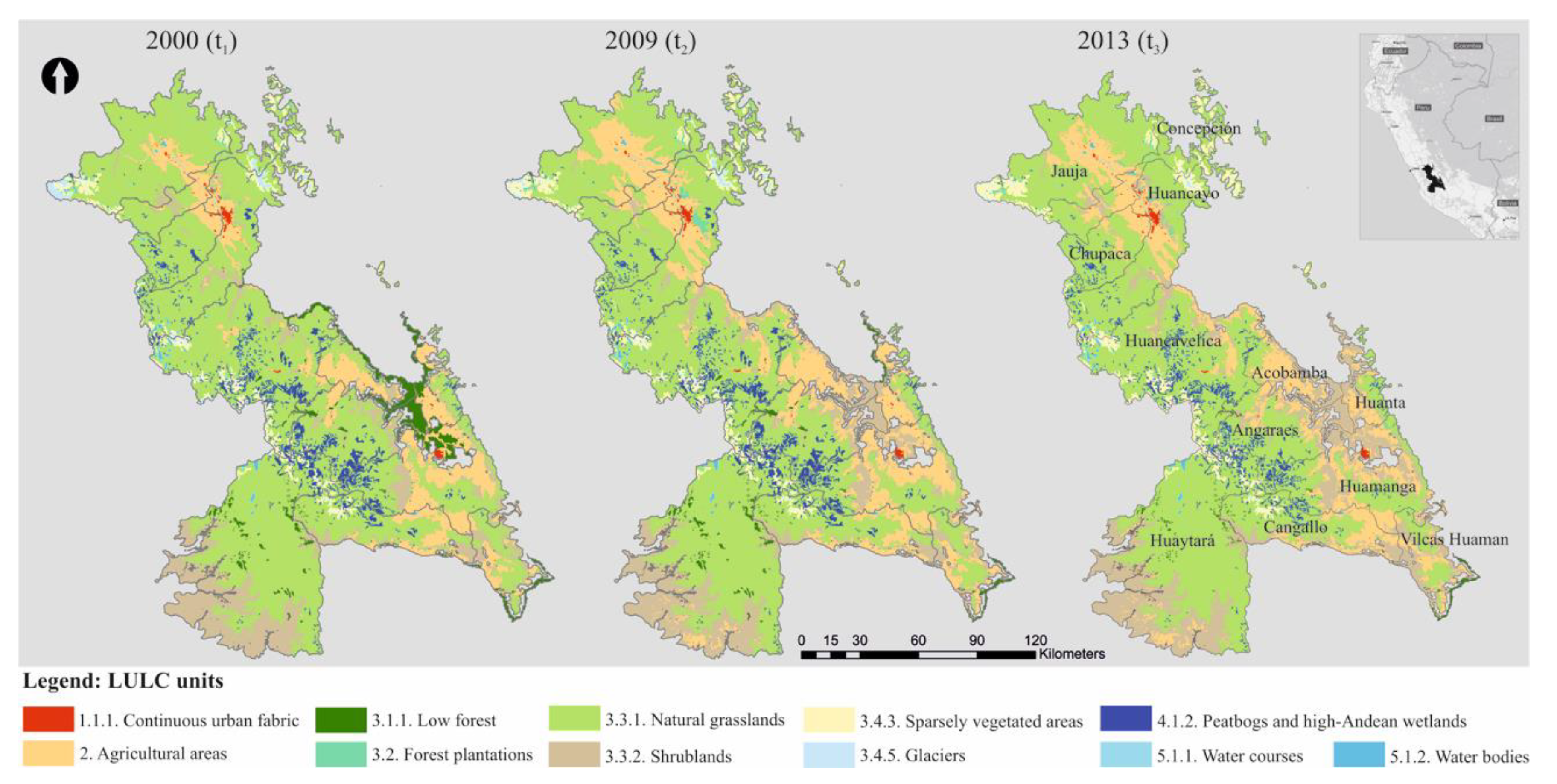
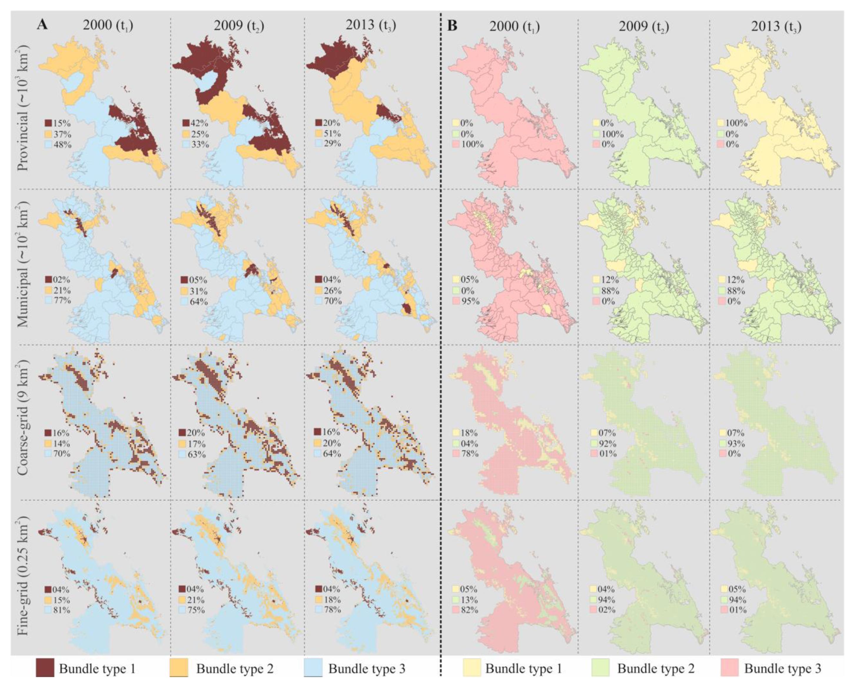
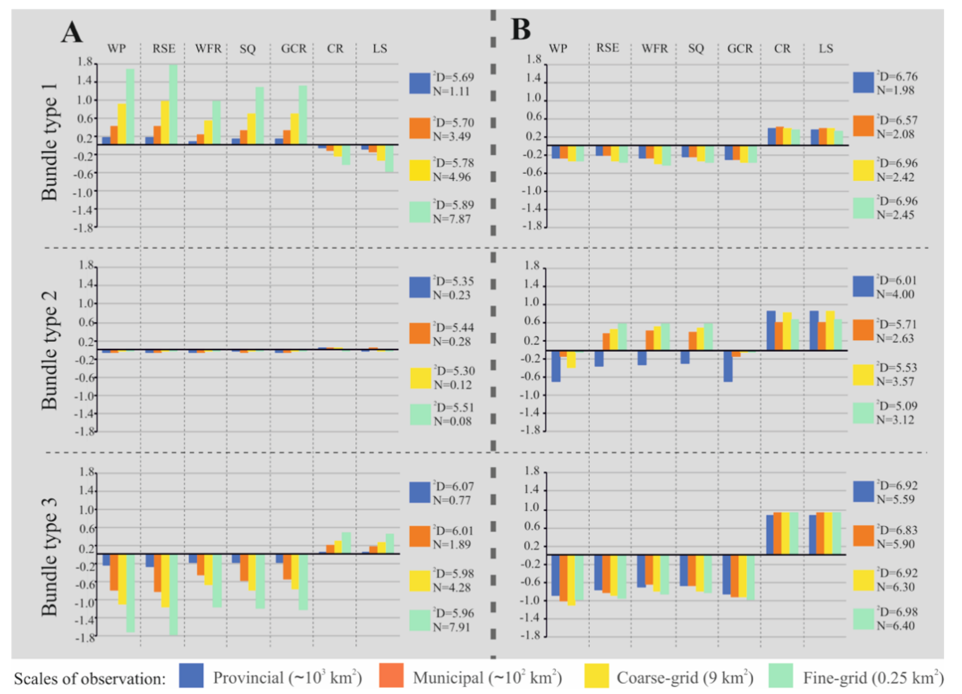
3.1. Static Cluster Analysis

The results of the two metrics used to evaluate the effects of the four spatial scales on the configuration of bundles showed similarities and disparities (Figure 2A). Regarding similarities, all the bundles provided an effective number of ES that ranged from 6.51 to 6.87. Concerning dissimilarities, most of the bundle types indicated disproportions among the abundance of ES. However, it showed a trend towards being higher for large spatial scales. Additionally, there was a trend of increasing of ES abundance from bundle type 1 to type 3 at each spatial resolution, but it had more similarities when the spatial scale increased. In that way, the provincial level was defined by the slight variation of ES values of the three bundle types. However, at the municipal level, type 3 was a multifunctional bundle, type 2 was a multifunctional agricultural bundle, and type 1 corresponded to an agriculture bundle. The coarse-grid scale mainly differed from the municipal in the bundle type 1 (agriculture and sparsely vegetated areas). However, at the fine-grid, the ES bundling showed a multifunctional bundle (type 3), an agriculture bundle (type 2), and an urban and sparsely vegetated area bundle (type 1).
The sensitivity analysis showed similarities between the effective number of ES provided by all the bundles, whereas the highest differences were detected among the abundance of bundles (Figure 2B). The diversity and the abundance of ES provided in bundles type 3 and type 2 was similar at the four scales of observation, whereas in type 1, differed. Thus, type 3 was a bundle with the highest values of regulating services, and type 2 was a bundle with the highest values in crop and livestock services. However, type 1 at the provincial level kept similarities with type 2, whereas at the municipal and grid scales had the lowest values of ES defined by urban and sparsely vegetated areas.
The spatial distribution of bundles obtained from ES values showed higher similarities among the three smaller spatial scales (Figure 3A). Thus, bundle type 3 dominated the territory (percentage of land >63%) over the three years. Nevertheless, the agricultural bundle had higher correspondences between grid-scales. At the provincial level, the three types of bundles were more evenly distributed (Figure 3A). The sensitivity analysis showed that the similarities between the spatial distribution of bundles followed a trend towards being higher for small spatial scales (Figure 3B). Then, at the municipal level and the two grid-scales, bundles kept fair spatial consistency across time, especially for types 2 and 3. On the contrary, at the provincial level, the territory was defined by a bundle type each year.
The analysis of historical trajectories showed that the bundle provided by any given land changed through time at each spatial scale but followed a decreasing trend from large to small (Table S8, Supplementary Materials). During the total study period, at the provincial level, 68% followed any trajectory of change, whereas this change was 30% at the municipal level. In the same way, the coarse-grid and fine-grid showed inferior variations of 24% and 14%, respectively. Furthermore, there was a second trend towards a higher number of transitions for fine spatial scales. These two trends were confirmed by the sensitivity analysis (Table S9, Supplementary Materials).

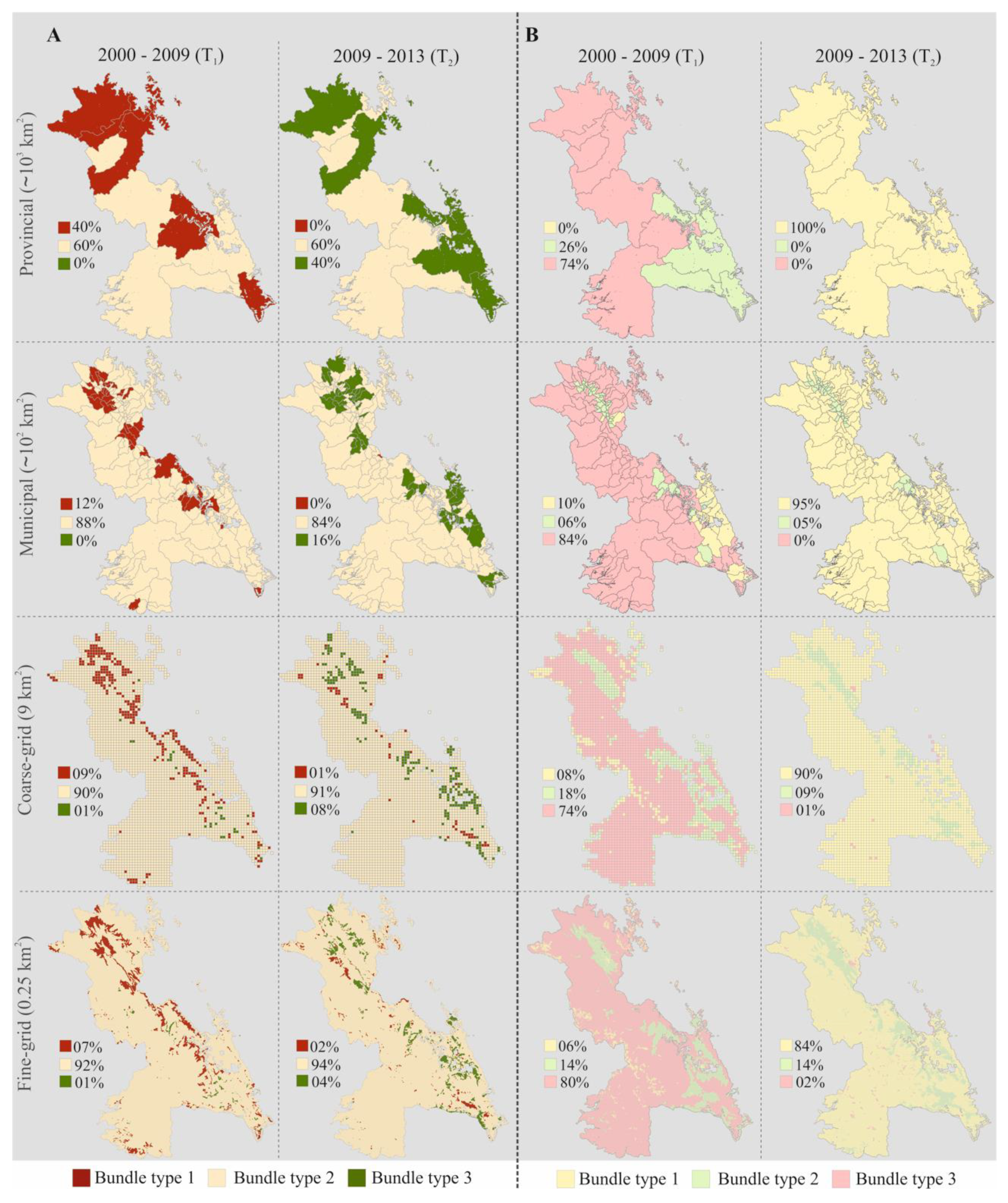
3.2. Dynamic Cluster Analysis

The analysis of the configuration of bundles at the four spatial scales presented similar measures of the effective number of ES changes (that ranged from 5.30 to 6.07), but differences in most of the N values (Figure 4A). Only bundle type 2 did not manifest these dissimilarities, since describing a territory without land-use change at the four spatial resolutions, remaining with similar and lowest N (almost 0). On the contrary, the N values specified by bundles type 1 and type 3 decreased when the spatial scale increased. In this regard, bundle type 1 revealed an increasing pattern from larger to smaller spatial scales, that detected the reduction in regulating services, and the increase in provisioning ES. However, bundle type 3 specified a trend of increase in provisioning services and a decrease in regulating.
For the sensitivity analysis, Figure 4B shows the similarities and the differences between the configuration of bundles across the four spatial scales. Similarities of the 2D metric are found for types 1 and 3, whereas type 2 showed higher differences across the four spatial scales. On the other hand, the N metric showed that for each bundle type, grid-scales had higher similarities between them and the municipality level. Furthermore, bundles type 1 and type 3 showed a consistent configuration of positive values of provisioning services and negative of regulating, whereas type 2 differed at the provincial level in the regulating services. Thus, bundles showed higher similarities among the three smaller spatial scales.
The spatial distribution of bundles across the two smaller spatial scales displayed a consistent pattern that began to be less evident at the provincial level (Figure 5A). In that sense, at the municipal level and on the two grid-scales, the territory seemed dominated by bundle type 2 (percentage of land >84%), whereas this percentage high declined at the provincial level. Likewise, the sensitivity analysis indicated fair robustness between municipal and grid-scales (Figure 5B). However, there were minor areas with changes in ES supply only detected at grid resolutions.
Historical trajectories of bundles achieved with ΔES values showed that the land that changed from one to another differed among spatial scales but was higher (52%) at the provincial level than at smaller levels (municipal: 24%; coarse-grid: 16%; fine-grid: 13%) (Table S10, Supplementary Materials). These transitions uncovered four main trajectories at all the spatial scales, and two more only found at the grid scales. Likewise, the sensitivity analysis showed that the proportion of land changing from one bundle to another was higher at the provincial level, and the number of trajectories was higher as the spatial scale decreased (Table S11, Supplementary Materials).

4. Discussion

In our study, the ES matrix contributes to the assessment of relationships between ES, applying two different methods (static and dynamic) across four scales of observation over time. At the spatial scale level, it revealed several findings consistent with those found by comparable biophysical assessment [16]. We analyzed the differences between each assessment method by comparing the results of standard metrics at each spatial scale over time. Subsequently, we discuss the main findings of the study validated by the sensitivity analysis (Table 2) and organized as scale and assessment method effects that might have implications on ES management.

4.1. Effects of Different Cluster Assessments on Bundles of ES

Depending on the cluster assessment, we found relationships between multiple ES that shifted in different ways. This finding agrees with previous work that also confirmed that the chosen method influences the result [6,20,42]. In that sense, in our study, “static bundles” suggested a positive spatial co-occurrence among the seven ES. On the contrary, “dynamic bundles” proposed a negative relationship between provisioning and regulating services. The synergy detected with the static assessment shows an opportunity to enhance multiple ES simultaneously. However, it missed the trade-off between regulating and provisioning services, and it could represent an unexpected loss of success for ES management. In fact, it implicates missing opportunities for win–win solutions that involve investments in conservation, restoration, and sustainable ecosystem use [64].
The spatial distribution of bundles captured by each cluster assessment showed differences. Thus, ES values displayed a landscape characterized by bundles with a specific diversity and abundance of ecosystem services supply at each time-step. On the other hand, ΔES values addressed the dynamics of ES bundles over the two time-periods. This last interpretation may facilitate the understanding of the instabilities that produce the temporal dynamics on ecosystems since trends expose whether there has been a change and the specified event that caused it [65]. This finding concerning “dynamic bundles” is consistent with previous research for the knowledge of land-changes dynamics [12].

4.2. Effects of Different Scales of Observation on Bundles of ES

The static assessment of bundles suggested that the configuration followed a trend towards more similarities at large spatial scales (Figure 2). This effect may explain that large spatial units follow a multifunctional landscape allowing relationships between ES to concur in synergy. It is understandable because the impacts of management actions at a fine-scale may be insignificant at a larger spatial scale if the land-use type affected is scarce, which is related to the capacity to capture local heterogeneity. Thus, the relationships between ES are conditioned by the geographical size of any single land-use change in the spatial unit. Consequently, at the grid scales, bundle types were more specialized according to one LULC unit (this was evident at the fine-grid scale). However, the provincial level provided a comparative abundance of ES because they were characterized by a similar combination of land-units. This similarity indicates comparable levels of land-use diversity that produces akin multifunctionality at large spatial units. Although multifunctionality is location related [66], this effect is observed in previous work of ES bundles across different administrative levels [16,24]. For instance, this generalization of the configuration can be inconvenient when we need to identify areas of highest/lowest supply of ES (hotspots/coldspots) for spatial prioritization or designing green infrastructure. For, as has been observed in our study site, the bundles of small size only persist across grid-scales. It implies a loss of bundle diversity when we upscale, which agrees with Zen et al. [67]. Then, large scales (dramatically at the provincial level) may fail to observe determinant factors and their influence on the sustainability of the ecosystems and their services. It reinforces the assumption that the increase in the spatial scale of observation brings a homogenization of the landscape [68], and only the mainland changes are significant [12].
At the three smaller spatial scales, bundles showed a similar configuration of positive and negative change in ES supply (Figure 4B), reflecting higher accuracy with the rate of change established by the different drivers (climate change, and technological improvement of agriculture and forestry). Needless to say, these bundles offer a basic view of the dynamic of ES that may help in planning win–win solutions. However, this basic picture depends on the size of the spatial unit, since it determines the intensity of drivers of change. In our study, as large as the spatial scale was, the land-use change impacts were more buffered. Although the provincial bundles detailed many similarities with the smaller scales of observation, the contrasts involve caution when using this spatial scale for the management of ecosystem services.
Static cluster analysis suggested high similarities between the spatial distribution of bundles at the municipal level and the two grid-scales. Consequently, it manifested fair robustness across the three smaller spatial scales, which differed with Raudsepp-Hearne and Peterson [16]. It may be related to the Andean study area, which is a landscape with ecosystem services more evenly distributed, and some amount of each ES facilitating multifunctionality can be found at the municipality level. Thus, the variation of bundling across a territory depends on the spatial heterogeneity of services since spatial homogeneity uncovers the same type of bundle across spatial scales. This diversity of findings recommends that researchers and decision-makers should be aware of the size and the heterogeneity of the spatial units to improve the aims of ES analyses [69]. Even though many times, there are limitations related to data scarcity or availability, which impede the research from being conducted optimally. We agree with previous research that considering at least two spatial scales should assure robustness [70,71], but we suggest a fine-grid scale and the municipality level. A fine-scale is important to show specific spots at local level that give a better panorama for well-informed planning decisions, whereas, at the municipality level is where political decisions are made and socioeconomic data are available. However, it is worth emphasizing that our study shows sufficient consistency between the municipal scale and the grid-scales.
The spatial distribution of bundles resulting from ΔES values revealed some consistency across spatial scales. However, bundling generalization was more evident as the scale of observation increased. This effect produces homogeneity at broad resolutions that can lead to shape a territory with similar land-use change intensity and overlooking fine-grained information needed for spatial conservation planning [72]. In our study site, at the provincial level, that generalization obscures changes in ecosystem services at lower levels that may be of importance for planning and management solutions. However, Madrigal-Martínez and Miralles i García [12] showed that, in research conditions of data scarcity, it is possible to address knowledge about land-change dynamics affecting ES that may help for policy and planning purposes at the provincial level.
For historical trajectories of bundles, both cluster analyses indicated that the area providing any given bundle changes higher at broad spatial scales over time. It implies that objects (land-units) within a large spatial unit are strongly associated, and a substantial change in one of them affects the total, whereas minor and static zones are overlooked. In our study area, this was more evident at the provincial level, in which the variation in ES supply of a given province was due to changes only in a few land-units. It is a consequence of upscaling that has direct impacts on the intensity of land-use change affecting ES. Low intense land-use change is not significant at broad scales [12]. In that sense, only at the grid-scales minor land-use changes that configured small size bundles were detected. This effect was detected in both cluster analyses and showed a trend towards a high number of trajectories for fine spatial scales. For example, we observe that bundles characterized by an increase in regulating services at grid-scales disappear at large (municipal and provincial). It reveals that changes at larger spatial scales have a buffer effect, whereas, at the fine-scales, bundles are more sensitive to temporal changes shaped by the direct local-scale drivers. This finding supports the assumption that knowledge of local contexts of ES is policy-relevant since their changes in values and demand are finer observable over time [73,74]. Therefore, the assessment of the spatial extension under the influence of drivers could help with the understanding of the stability of ES provision, endorsing robustness for the development of sustainable management and conservation strategies.

4.3. Methodological Limitations

In this study, the analyses presented should be understood as using the best existing data of an acceptable quality to admit a robust demonstration. Even so, the method (ES matrix) brings potential limitations to the study, and technical and thematic uncertainties [75]. In that sense, we highlight that the capacity matrix simplifies landscape functionality producing uncertainties in the quantification of ES (e.g., regulating services). It is due to this that some ES are not only dependent on the presence of certain land use/land cover types but also their spatial configuration. Moreover, management actions on each land-use may affect ES flow differently (specially in provisioning services), and this effect could be measured vaguely for the matrix. Another limitation lies in that the reduced and diverse data sources of land use/land cover classes made a generalization of the landscape necessary, which could influence the bundles that emerge at larger spatial scales. In fact, a more precise number of land use/land cover classes could result in the reconfiguration of bundles [69]. Additionally, in ES matrix models, the multifunctionality is strongly dependent on the number of services provided by the different land use/land cover types [76]. On the other hand, when data at a fine-scale were summarized at the administrative levels (aggregation effect), they could cause a loss of information [77]. Finally, the data source (the map of high-Andean ecosystems) has a vague delimitation for two land units (agricultural areas and forest plantation), comprehending them in only one land-use category (Areas modified by human action). However, we considered this limitation of minor importance because this aspect was clarified using the land-use types from the two official flora cover maps.

5. Conclusions

We developed a study that addressed the effects of different cluster methods for assessing bundles of ES across different scales of observation over time, using an example in the high-Andean moist Puna. We aimed to detect the differences in applying two cluster analyses—for ES values and ΔES values—and the effects of different scales of observation—two administrative levels and two grid resolutions—on ES bundles over time. To address these objectives, we investigated two hypotheses: (1) bundles of ES differ on the method applied for assessing them; (2) these bundles are affected by the scale of observation. Our analysis uncovered consistent differences suggesting that the selection of a method for assessing bundles of ES might define the results, and the scale of observation influenced them.
“Static” bundles suggested synergies between provisioning and regulating services, whereas “dynamic” indicated negative relationships. Then, the assumption of a general pattern of trade-offs between these groups of services needs to be analyzed in detail [27,42]. The diverse interpretations found in our study suggest that both assessment methods have implications for management of ES, and both can be complementary to obtain better contributions for decision-making. However, if research objectives are focused on the understanding of the instabilities that produce the temporal dynamics on ecosystems, we recommend the assessment of “dynamic” bundles since these are more sensitive to changes of the different drivers across spatial scales. Moreover, any spatial scale can be eligible, but large administrative levels need caution.
The differences addressed over time showed confident generalization to advise the pros and cons of which spatial scale to use. The municipality level showed sufficient consistency with grid-scales, which may be enough to guide policy, as other studies highlighted [16,28]. However, for spatial conservation, the fine-grid scale could be needed to visualize small patch sizes. Then, as a rule, resulting from the study, ES bundles at grid scales characterized by a high level of dispersion and small patch size disappear or are imperceptible at administrative levels. Indeed, at heterogeneous landscapes, bundling becomes complex, whereas bundles are very similar across different spatial scales on homogeneous landscapes. In that sense, bundles at administrative levels tend to describe landscape multifunctionality, whereas fine-grained resolutions define more specialized bundles.
Finally, we have shown that the ES matrix and standard metrics give guidance to show the implications of choosing a method and a scale of observation in bundle assessment. To the best of our knowledge, this is the first study in which such a comprehensive step by step framework comparing “dynamic” and “static” bundles of ES has been developed. Bearing in mind the potential of bundles to support decision-making, the results might help the choice of bundling methods during the design of research projects. Our findings fill the knowledge gap on relationships between multiple ES utilizing cluster techniques robustly. Future studies should focus on a much more exhaustive list of ES. Additionally, more research is required to assess bundles at different spatial extensions and on landscapes with diverse levels of spatial heterogeneity.

Supplementary Materials

The following are available online at https://www.mdpi.com/2073-445X/9/10/392/s1. Supplementary Materials, including Tables S1–S4, Figure S5, and Tables S6–S11 are included in a separate file.

Author Contributions

Conceptualization, S.M.-M. and J.L.M.i.G.; Methodology, S.M.-M.; Software, S.M.-M.; Validation, S.M.-M. and J.L.M.i.G.; Formal Analysis, S.M.-M.; Investigation, S.M.-M.; Resources, S.M.-M.; Data Curation, S.M.-M.; Writing—Original Draft Preparation, S.M.-M.; Writing—Review and Editing, S.M.-M. and J.L.M.i.G.; Visualization, S.M.-M.; Supervision, J.L.M.i.G.; Funding Acquisition, J.L.M.i.G. All authors have read and agreed to the published version of the manuscript.

Funding

This research received no external funding.

Acknowledgments

The authors would like to thank the five experts for providing specialist judgment for the development of the sensitivity scenario. Additionally, we thank the subject editor and four anonymous reviewers for their valuable comments and suggestions.

Conflicts of Interest

The authors declare no conflict of interest.

References

  1. Millennium Ecosystem Assessment. Ecosystems and Human Well-Being: Synthesis; Millennium Ecosystem Assessment: Washington, DC, USA, 2005. [Google Scholar]
  2. Liu, J.; Mooney, H.A.; Hull, V.; Davis, S.J.; Gaskell, J.; Hertel, T.W.; Lubchenco, J.; Seto, K.C.; Gleick, P.; Kremen, C.; et al. Systems integration for global sustainability. Science 2015, 347, 1258832. [Google Scholar] [CrossRef] [PubMed] [Green Version]
  3. Abson, D.J.; Von Wehrden, H.; Baumgärtner, S.; Fischer, J.; Hanspach, J.; Härdtle, W.; Heinrichs, H.; Klein, A.M.; Lang, D.J.; Martens, P.; et al. Ecosystem services as a boundary object for sustainability. Ecol. Econ. 2014, 103, 29–37. [Google Scholar] [CrossRef]
  4. Spellerberg, I.; Vos, C.C.; Opdam, P. Landscape Ecology of a Stressed Environment. J. Ecol. 1993, 81, 599. [Google Scholar] [CrossRef]
  5. Vihervaara, P.; Rönkä, M.; Walls, M. Trends in Ecosystem Service Research: Early Steps and Current Drivers. Ambio 2010, 39, 314–324. [Google Scholar] [CrossRef] [PubMed]
  6. Lee, H.; Lautenbach, S. A quantitative review of relationships between ecosystem services. Ecol. Indic. 2016, 66, 340–351. [Google Scholar] [CrossRef]
  7. Mouchet, M.A.; Lamarque, P.; Martín-López, B.; Crouzat, E.; Gos, P.; Byczek, C.; Lavorel, S. An interdisciplinary methodological guide for quantifying associations between ecosystem services. Glob. Environ. Chang. 2014, 28, 298–308. [Google Scholar] [CrossRef]
  8. Cord, A.F.; Bartkowski, B.; Beckmann, M.; Dittrich, A.; Hermans-Neumann, K.; Kaim, A.; Lienhoop, N.; Locher-Krause, K.; Priess, J.; Schröter-Schlaack, C.; et al. Towards systematic analyses of ecosystem service trade-offs and synergies: Main concepts, methods and the road ahead. Ecosyst. Serv. 2017, 28, 264–272. [Google Scholar] [CrossRef]
  9. Howe, C.; Suich, H.; Vira, B.; Mace, G.M. Creating win-wins from trade-offs? Ecosystem services for human well-being: A meta-analysis of ecosystem service trade-offs and synergies in the real world. Glob. Environ. Chang. 2014, 28, 263–275. [Google Scholar] [CrossRef] [Green Version]
  10. Deng, X.; Li, Z.; Gibson, J. A review on trade-off analysis of ecosystem services for sustainable land-use management. J. Geogr. Sci. 2016, 26, 953–968. [Google Scholar] [CrossRef] [Green Version]
  11. Renard, D.; Rhemtulla, J.M.; Bennett, E.M. Historical dynamics in ecosystem service bundles. Proc. Natl. Acad. Sci. USA 2015, 112, 13411–13416. [Google Scholar] [CrossRef] [Green Version]
  12. Madrigal-Martínez, S.; Miralles i García, J.L. Land-change dynamics and ecosystem service trends across the central high-Andean Puna. Sci. Rep. 2019, 9, 9688. [Google Scholar] [CrossRef] [PubMed] [Green Version]
  13. Stürck, J.; Schulp, C.; Verburg, P.H. Spatio-temporal dynamics of regulating ecosystem services in Europe—The role of past and future land use change. Appl. Geogr. 2015, 63, 121–135. [Google Scholar] [CrossRef]
  14. Hou, Y.; Lü, Y.; Chen, W.; Fu, B. Temporal variation and spatial scale dependency of ecosystem service interactions: A case study on the central Loess Plateau of China. Landsc. Ecol. 2017, 32, 1201–1217. [Google Scholar] [CrossRef]
  15. Xu, S.; Liu, Y.; Wang, X.; Zhang, G. Scale effect on spatial patterns of ecosystem services and associations among them in semi-arid area: A case study in Ningxia Hui Autonomous Region, China. Sci. Total. Environ. 2017, 598, 297–306. [Google Scholar] [CrossRef]
  16. Raudsepp-Hearne, C.; Peterson, G.D. Scale and ecosystem services: How do observation, management, and analysis shift with scale—lessons from Québec. Ecol. Soc. 2016, 21. [Google Scholar] [CrossRef] [Green Version]
  17. Rodriguez, L.C.; Pascual, U.; Niemeyer, H.M. Local identification and valuation of ecosystem goods and services from Opuntia scrublands of Ayacucho, Peru. Ecol. Econ. 2006, 57, 30–44. [Google Scholar] [CrossRef]
  18. Bennett, E.M.; Peterson, G.D.; Gordon, L.J. Understanding relationships among multiple ecosystem services. Ecol. Lett. 2009, 12, 1394–1404. [Google Scholar] [CrossRef]
  19. Raudsepp-Hearne, C.; Peterson, G.D.; Bennett, E.M. Ecosystem service bundles for analyzing tradeoffs in diverse landscapes. Proc. Natl. Acad. Sci. USA 2010, 107, 5242–5247. [Google Scholar] [CrossRef] [Green Version]
  20. Tomscha, S.; Gergel, S.E. Ecosystem service trade-offs and synergies misunderstood without landscape history. Ecol. Soc. 2016, 21. [Google Scholar] [CrossRef] [Green Version]
  21. Lavorel, S.; Bayer, A.; Bondeau, A.; Lautenbach, S.; Ruiz-Frau, A.; Schulp, N.; Seppelt, R.; Verburg, P.; Van Teeffelen, A.; Vannier, C.; et al. Pathways to bridge the biophysical realism gap in ecosystem services mapping approaches. Ecol. Indic. 2017, 74, 241–260. [Google Scholar] [CrossRef] [Green Version]
  22. Li, T.; Lü, Y.; Fu, B.; Hu, W.; Comber, A. Bundling ecosystem services for detecting their interactions driven by large-scale vegetation restoration: Enhanced services while depressed synergies. Ecol. Indic. 2019, 99, 332–342. [Google Scholar] [CrossRef] [Green Version]
  23. Fan, W.; Fan, W.; Lu, N.; Xu, Z.; Liu, H.; Chen, W.; Ulgiati, S.; Wang, X.; Dong, X. Integrating Biophysical and Sociocultural Methods for Identifying the Relationships between Ecosystem Services and Land Use Change: Insights from an Oasis Area. Sustainability 2019, 11, 2598. [Google Scholar] [CrossRef] [Green Version]
  24. Hamann, M.; Biggs, R.; Reyers, B. Mapping social–ecological systems: Identifying ‘green-loop’ and ‘red-loop’ dynamics based on characteristic bundles of ecosystem service use. Glob. Environ. Chang. 2015, 34, 218–226. [Google Scholar] [CrossRef]
  25. Dou, H.; Li, X.; Li, S.; Dang, D. How to Detect Scale Effect of Ecosystem Services Supply? A Comprehensive Insight from Xilinhot in Inner Mongolia, China. Sustainability 2018, 10, 3654. [Google Scholar] [CrossRef] [Green Version]
  26. Cui, F.; Tang, H.; Zhang, Q.; Wang, B.; Dai, L. Integrating ecosystem services supply and demand into optimized management at different scales: A case study in Hulunbuir, China. Ecosyst. Serv. 2019, 39, 39. [Google Scholar] [CrossRef]
  27. Qiao, X.; Gu, Y.; Zou, C.; Xu, D.; Wang, L.; Ye, X.; Yang, Y.; Huang, X. Temporal variation and spatial scale dependency of the trade-offs and synergies among multiple ecosystem services in the Taihu Lake Basin of China. Sci. Total. Environ. 2019, 651, 218–229. [Google Scholar] [CrossRef]
  28. Roces-Díaz, J.V.; Vayreda, J.; Banqué-Casanovas, M.; Díaz-Varela, E.; Bonet, J.A.; Brotons, L.; De Miguel, S.; Herrando, S.; Martinez-Vilalta, J. The spatial level of analysis affects the patterns of forest ecosystem services supply and their relationships. Sci. Total. Environ. 2018, 626, 1270–1283. [Google Scholar] [CrossRef] [PubMed] [Green Version]
  29. Spake, R.; Lasseur, R.; Crouzat, E.; Bullock, J.M.; Lavorel, S.; Parks, K.E.; Schaafsma, M.; Bennett, E.M.; Maes, J.; Mulligan, M.; et al. Unpacking ecosystem service bundles: Towards predictive mapping of synergies and trade-offs between ecosystem services. Glob. Environ. Chang. 2017, 47, 37–50. [Google Scholar] [CrossRef] [Green Version]
  30. Dade, M.C.; Mitchell, M.G.; McAlpine, C.A.; Rhodes, J.R. Assessing ecosystem service trade-offs and synergies: The need for a more mechanistic approach. Ambio 2018, 48, 1116–1128. [Google Scholar] [CrossRef]
  31. Saidi, N.; Spray, C.J. Ecosystem services bundles: Challenges and opportunities for implementation and further research. Environ. Res. Lett. 2018, 13, 113001. [Google Scholar] [CrossRef]
  32. Crouzat, E.; Mouchet, M.; Turkelboom, F.; Byczek, C.; Meersmans, J.; Berger, F.; Verkerk, P.J.; Lavorel, S. Assessing bundles of ecosystem services from regional to landscape scale: Insights from the French Alps. J. Appl. Ecol. 2015, 52, 1145–1155. [Google Scholar] [CrossRef] [Green Version]
  33. Van Der Biest, K.; D’Hondt, R.; Jacobs, S.; Landuyt, D.; Staes, J.; Goethals, P.; Meire, P. EBI: An index for delivery of ecosystem service bundles. Ecol. Indic. 2014, 37, 252–265. [Google Scholar] [CrossRef]
  34. Egoh, B.N.; Reyers, B.; Rouget, M.; Richardson, D.M. Identifying priority areas for ecosystem service management in South African grasslands. J. Environ. Manag. 2011, 92, 1642–1650. [Google Scholar] [CrossRef] [Green Version]
  35. Martín-López, B.; Iniesta-Arandia, I.; García-Llorente, M.; Palomo, I.; Casado-Arzuaga, I.; Del Amo, D.G.; Gómez-Baggethun, E.; Oteros-Rozas, E.; Palacios-Agundez, I.; Willaarts, B.; et al. Uncovering Ecosystem Service Bundles through Social Preferences. PLoS ONE 2012, 7, e38970. [Google Scholar] [CrossRef] [Green Version]
  36. Yang, G.; Ge, Y.; Xue, H.; Yang, W.; Shi, Y.; Peng, C.; Du, Y.; Fan, X.; Ren, Y.; Chang, S.X. Using ecosystem service bundles to detect trade-offs and synergies across urban–rural complexes. Landsc. Urban Plan. 2015, 136, 110–121. [Google Scholar] [CrossRef]
  37. Queiroz, C.; Meacham, M.; Richter, K.; Norström, A.V.; Andersson, E.; Norberg, J.; Peterson, G.D. Mapping bundles of ecosystem services reveals distinct types of multifunctionality within a Swedish landscape. Ambio 2015, 44, 89–101. [Google Scholar] [CrossRef] [Green Version]
  38. Turner, K.G.; Odgaard, M.V.; Bøcher, P.K.; Dalgaard, T.; Svenning, J.-C. Bundling ecosystem services in Denmark: Trade-offs and synergies in a cultural landscape. Landsc. Urban Plan. 2014, 125, 89–104. [Google Scholar] [CrossRef]
  39. Kühne, O.; Duttmann, R. Recent Challenges of the Ecosystems Services Approach from an Interdisciplinary Point of View. Raumforsch. Raumordn. 2019, 171–184. [Google Scholar] [CrossRef]
  40. Birkhofer, K.; Diehl, E.; Andersson, J.; Ekroos, J.; Früh-Müller, A.; Machnikowski, F.; Mader, V.L.; Nilsson, L.; Sasaki, K.; Rundlöf, M.; et al. Ecosystem services-current challenges and opportunities for ecological research. Front. Ecol. Evol. 2015, 2. [Google Scholar] [CrossRef] [Green Version]
  41. Rieb, J.T.; Chaplin-Kramer, R.; Daily, G.C.; Armsworth, P.R.; Böhning-Gaese, K.; Bonn, A.; Cumming, G.S.; Eigenbrod, F.; Grimm, V.; Jackson, B.M.; et al. When, Where, and How Nature Matters for Ecosystem Services: Challenges for the Next Generation of Ecosystem Service Models. Bioscience 2017, 67, 820–833. [Google Scholar] [CrossRef]
  42. Vallet, A.; Locatelli, B.; Levrel, H.; Wunder, S.; Seppelt, R.; Scholes, R.J.; Oszwald, J. Relationships Between Ecosystem Services: Comparing Methods for Assessing Tradeoffs and Synergies. Ecol. Econ. 2018, 150, 96–106. [Google Scholar] [CrossRef]
  43. Zheng, Z.; Fu, B.; Hu, H.; Sun, G. A method to identify the variable ecosystem services relationship across time: A case study on Yanhe Basin, China. Landsc. Ecol. 2014, 29, 1689–1696. [Google Scholar] [CrossRef] [Green Version]
  44. Madrigal-Martinez, S.; Miralles i García, J.L. Understanding land use changes in the central high-Andean moist Puna. WIT Trans. Ecol. Environ 2019, 238, 175–186. [Google Scholar] [CrossRef]
  45. Josse, C.; Cuesta, F.; Navarro, G.; Barrena, V.; Cabrera, E.; Chacón-Moreno, E.; Ferreira, W.; Peralvo, M.; Saito, J.; Tovar, A. Andean Ecosystems of the North and the Center; Secretaría General de la Comunidad Andina, Programa Regional ECOBONA-Intercooperation, CONDESAN-Proyecto Páramo Andino, Programa BioAndes, EcoCiencia, NatureServe, IAvH, LTA-UNALM, ICAE-ULA, CDC-UNALM, RUMBOL SRL: Lima, Peru, 2009; p. 100. [Google Scholar]
  46. Young, K.R. Andean land use and biodiversity: Humanized landscapes in a time of change. Ann. Mo. Bot. Gard. 2009, 96, 492–507. [Google Scholar] [CrossRef] [Green Version]
  47. Madrigal-Martínez, S.; Miralles i García, J.L. Ecosystem Services in Peru: Threats, Opportunities and Their Importance for the High-Andean Moist Puna. In Peru in the 21st Century: Progress, Trends and Challenges; Mariela Noles Cotito, Ed.; Nova Science Publishers: New York, NY, USA, 2020; ISBN 9781536184983. [Google Scholar]
  48. Jacobs, S.; Burkhard, B.; Van Daele, T.; Staes, J.; Schneiders, A. ‘The Matrix Reloaded’: A review of expert knowledge use for mapping ecosystem services. Ecol. Model. 2015, 295, 21–30. [Google Scholar] [CrossRef]
  49. Campagne, C.S.; Roche, P.; Müller, F.; Burkhard, B. Ten years of ecosystem services matrix: Review of a (r)evolution. One Ecosyst. 2020, 5, e51103. [Google Scholar] [CrossRef]
  50. Burkhard, B.; Kandziora, M.; Hou, Y.; Müller, F. Ecosystem service potentials, flows and demands-concepts for spatial localisation, indication and quantification. Landsc. Online 2014, 34, 1–32. [Google Scholar] [CrossRef]
  51. Drescher, M.; Perera, A.H.; Johnson, C.J.; Buse, L.J.; Drew, C.A.; Burgman, M.A. Toward rigorous use of expert knowledge in ecological research. Ecosphere 2013, 4, 83. [Google Scholar] [CrossRef]
  52. Roche, P.K.; Campagne, C.S. Are expert-based ecosystem services scores related to biophysical quantitative estimates? Ecol. Indic. 2019, 106, 105421. [Google Scholar] [CrossRef]
  53. Jacobs, S.; Burkhard, B. Applying expert knowledge for ecosystem services quantification. In Mapping Ecosystem Services; Burkhard, B., Maes, J., Eds.; Pensoft Publishers: Sofia, Bulgaria, 2017; p. 374. [Google Scholar]
  54. INEI—National Institute of Statistics and Informatics National census. Available online: https://www.inei.gob.pe/estadisticas/censos/ (accessed on 13 January 2020).
  55. Ministry of Environment. Technical Report of the Peruvian Map of Flora Cover; Ministry of Environment: Lima, Peru, 2012; ISBN 9786124605369. [Google Scholar]
  56. Ministry of Environment. Peruvian National Map of Flora Cover; Ministry of Environment: Lima, Peru, 2015; p. 1. [Google Scholar]
  57. Haines-Young, R.; Potschin, M. Common International Clasification of Ecosystem Services CICES V5. 1. Guidance on the Application of the Revised Structure. Fabis Consult. 2018, 53. [Google Scholar]
  58. Ryden, K. Environmental Systems Research Institute Mapping. Am. Cartogr. 1987, 14, 261–263. [Google Scholar] [CrossRef]
  59. Charrad, M.; Ghazzali, N.; Boiteau, V.; Niknafs, A. Package ‘NbClust’. NbClust: An R Package for Determining the Relevant Number of Clusters in a Data Set. J. Stat. Softw. 2014, 61, 1–36. Available online: http://www.jstatsoft.org/v61/i06/ (accessed on 10 February 2020). [CrossRef] [Green Version]
  60. Development Core Team. R: A Language and Environment for Statistical Computing. R Found. Stat. Comput. 2016, 1, 409. [Google Scholar]
  61. Hill, M.O. Diversity and Evenness: A Unifying Notation and Its Consequences. Ecology 1973, 54, 427–432. [Google Scholar] [CrossRef] [Green Version]
  62. Jost, L. Entropy and diversity. Oikos 2006, 113, 363–375. [Google Scholar] [CrossRef]
  63. Metzger, M.J.; Rounsevell, M.D.A.; Heiligenberg, H.A.V.D.; Pérez-Soba, M.; Hardiman, P.S. How Personal Judgment Influences Scenario Development: An Example for Future Rural Development in Europe. Ecol. Soc. 2010, 15, 27. [Google Scholar] [CrossRef]
  64. De Groot, R.; Alkemade, R.; Braat, L.; Hein, L.; Willemen, L. Challenges in integrating the concept of ecosystem services and values in landscape planning, management and decision making. Ecol. Complex. 2010, 7, 260–272. [Google Scholar] [CrossRef]
  65. De Gruijter, J.J.; Bierkens, M.F.P.; Brus, D.J.; Knotters, M. Sampling for Natural Resource Monitoring. Sampling for Natural Resource Monitoring; Springer: Berlin/Heidelberg, Germany, 2006. [Google Scholar]
  66. Stürck, J.; Verburg, P.H. Multifunctionality at what scale? A landscape multifunctionality assessment for the European Union under conditions of land use change. Landsc. Ecol. 2016, 32, 481–500. [Google Scholar] [CrossRef] [Green Version]
  67. Zen, M.; Candiago, S.; Schirpke, U.; Vigl, L.E.; Giupponi, C.; Michele, Z.; Sebastian, C.; Uta, S.; Lukas, E.V.; Carlo, G. Upscaling ecosystem service maps to administrative levels: Beyond scale mismatches. Sci. Total. Environ. 2019, 660, 1565–1575. [Google Scholar] [CrossRef]
  68. Turner, M.G.; O’Neill, R.V.; Gardner, R.H.; Milne, B.T. Effects of changing spatial scale on the analysis of landscape pattern. Landsc. Ecol. 1989, 3, 153–162. [Google Scholar] [CrossRef]
  69. Verhagen, W.; Van Teeffelen, A.J.A.; Compagnucci, A.B.; Poggio, L.; Gimona, A.; Verburg, P.H. Effects of landscape configuration on mapping ecosystem service capacity: A review of evidence and a case study in Scotland. Landsc. Ecol. 2016, 31, 1457–1479. [Google Scholar] [CrossRef]
  70. Scholes, R.; Reyers, B.; Biggs, R.; Spierenburg, M.; Duriappah, A. Multi-scale and cross-scale assessments of social–ecological systems and their ecosystem services. Curr. Opin. Environ. Sustain. 2013, 5, 16–25. [Google Scholar] [CrossRef]
  71. Felipe-Lucia, M.R.; Comín, F.A.; Bennett, E.M. Interactions Among Ecosystem Services Across Land Uses in a Floodplain Agroecosystem. Ecol. Soc. 2014, 19. [Google Scholar] [CrossRef] [Green Version]
  72. Trabucchi, M.; Comín, F.A.; O’Farrell, P.J. Hierarchical priority setting for restoration in a watershed in NE Spain, based on assessments of soil erosion and ecosystem services. Reg. Environ. Chang. 2013, 13, 911–926. [Google Scholar] [CrossRef] [Green Version]
  73. Pandeya, B.; Buytaert, W.; Zulkafli, Z.; Karpouzoglou, T.; Mao, F.; Hannah, D. A comparative analysis of ecosystem services valuation approaches for application at the local scale and in data scarce regions. Ecosyst. Serv. 2016, 22, 250–259. [Google Scholar] [CrossRef] [Green Version]
  74. Hein, L.; Van Koppen, C. (Kris); Van Ierland, E.C.; Leidekker, J. Temporal scales, ecosystem dynamics, stakeholders and the valuation of ecosystems services. Ecosyst. Serv. 2016, 21, 109–119. [Google Scholar] [CrossRef]
  75. Hou, Y.; Burkhard, B.; Müller, F. Uncertainties in landscape analysis and ecosystem service assessment. J. Environ. Manag. 2013, 127, S117–S131. [Google Scholar] [CrossRef] [PubMed]
  76. Burkhard, B.; Kroll, F.; Müller, F.; Windhorst, W. Landscapes’ capacities to provide ecosystem services—A concept for land-cover based assessments. Landsc. Online 2009, 15, 1–22. [Google Scholar] [CrossRef]
  77. Bolliger, J.; Mladenoff, D.J. Quantifying spatial classification uncertainties of the historical Wisconsin landscape (USA). Ecography 2005, 28, 141–156. [Google Scholar] [CrossRef]
Figure 1. The 12 provinces in the central high-Andean moist Puna over time. The maps display the land use/land cover (LULC) units for each time step from 2000 to 2013. The map at the right-top shows the location of the study site in Peru.
Land 09 00392 g001
Figure 2. Configuration of bundles and metrics derived from ES values (A) and the sensitivity analysis (B) at the four spatial scales. Spider charts illustrate the abundance of ES potential supplied by each bundle. Each axe length is proportional to the relative abundances of the other ES within each bundle (axes are comparable within bundles). Metrics and abbreviations: true diversity (2D), and abundance (N). Ecosystem service types and abbreviations: water purification (WP), regulation of soil erosion (RSE), water flow regulation (WFR), soil quality (SQ), global climate regulation (GCR), crops (CR) and livestock (LS).
Land 09 00392 g002
Figure 3. Spatial distribution of bundles resulting from ES values (A) and the sensitivity analysis (B) across the four spatial scales over the three years. Maps show the spatial distribution and proportion of land of each bundle over time and across each spatial scale.
Land 09 00392 g003
Figure 4. Configuration of bundles and metrics derived from ΔES values (A) and the sensitivity analysis (B) at the four spatial scales. Bar plots show the amount of change in ES values at two times within each bundle type. Each bar length is proportional to the relative abundances of the other ΔES values within each bundle (bars are comparable within bundles). Metrics and abbreviations: true diversity (2D), and abundance (N). Ecosystem service types and abbreviations: water purification (WP), regulation of soil erosion (RSE), water flow regulation (WFR), soil quality (SQ), global climate regulation (GCR), crops (CR) and livestock (LS).
Land 09 00392 g004
Figure 5. Spatial distribution of bundles resulting from ΔES values (A) and the sensitivity analysis (B) across the four spatial scales at each period. Maps show the spatial distribution and proportion of land of each bundle over the two-time periods and across each spatial scale.
Land 09 00392 g005
Table 1. Metrics (and their description) used for the achievement of the aspects of bundles.
AspectMetricDescription
ConfigurationTrue Diversity (Order 2) (2D)The diversity of a set of ES provided in a given bundle type is calculated as the effective number of ecosystem services based on Hill numbers [61,62]. For the “dynamic bundles”, we used the absolute value of each amount of change in ES specified by a given bundle. This metric was included because it affords a stable, clearly understood, and sensitive overall similarity measure supporting cross-study assessments [11,62].
Abundance (N)The sum of the absolute value of each ES (or ΔES) specified by a given bundle type. The sum represents an overall level of the provisioning of services (or of the change in services). High absolute values thus indicate zones with a comparatively high supply of (or change in) multiple services, while low values indicate the opposite. This metric was included in the bundle analysis because policies are intended to protect the overall level of ES provision rather than, or in addition, to the provision of individual services.
Spatial patternsPercentage of landThe proportional abundance of a given bundle type in a given year or a given period across the study area. It is a landscape metric that acts as a proxy for change, thus allowing for the interpretation of spatial patterns over time and space. This metric measured the results of both cluster analyses.
Historical trajectoriesPercentage of land changeThe proportion of land changing from one bundle in a year or period t to another in a year or period t+1 on the same spatial scale. This metric measured the results of both cluster analyses.
Table 2. Scale and assessment method effects on bundles of ecosystem services.
Assessment Method EffectSpatial Scale Effect
  • Configuration: disagreement in the direction of the relationships between multiple ES.
  • Spatial patterns: static cluster analysis captured only a snapshot of ES bundles at different years, whereas cluster analysis with ΔES values displayed dynamics of ES bundles.
  • Configuration: static cluster analysis displayed a trend towards more similarities among bundle types for large spatial scales, whereas dynamic cluster analysis showed a similar trend of positive and negative change in the ES supply at the three smaller spatial scales.
  • Spatial patterns: static cluster analysis suggested higher similarities between bundles at the municipal level and the two grid-scales, whereas dynamic cluster analysis showed some consistency across spatial scales.
  • Historical trajectories: both cluster analyses detected: (1) a trend towards a high percentage of land change for large spatial scales, and (2) a trend towards a high number of trajectories for fine spatial scales.
Publisher’s Note: MDPI stays neutral with regard to jurisdictional claims in published maps and institutional affiliations.

