Carbon Storage Dynamics and Multi-Scenario Territorial Regulation in South China’s Karst-Coastal Transition Zones Under the “Dual Carbon” Target

Abstract

In the context of low-carbon development targets, urban expansion within the karst ecoregions of southern China has intensified land-use-related carbon-stock losses, which highlights the necessity of scientific and sustainable land-use management strategies. Using multi-temporal land-use datasts spanning six periods from 2000 to 2025, this study integrates carbon-stock accounting and land-use transition-matrix analysis. Multicollinearity testing and spatial autocorrelation analysis are employed to reveal the driving mechanisms behind carbon-stock variations. Based on standardized beta coefficients (β), all driving factors are hierarchically classified into primary dominant factors, secondary constraint factors, and tertiary disturbance factors according to their regulatory intensity, and further grouped into topographic, ecological, and socioeconomic categories. On this basis, three differentiated land-management scenarios are constructed. By coupling the PLUS and InVEST models, this study simulates regional carbon-stock conditions for 2030 and 2035. The results show that regional carbon-stock exhibits a fluctuating pattern: it decreased from 2000 to 2005, rose continuously during 2005–2015 to reach its peak in 2015, and then declined persistently from 2015 to 2025. Spatially, obvious zonal differentiation can be observed: the northwestern mountainous areas maintain high carbon-stock levels, whereas southern coastal towns experience severe carbon-stock degradation. Topographic factors dominate regional carbon-stock dynamics; ecological factors exert critical buffering effects; human-induced land-use activities act as the secondary driver for carbon-stock loss. The conversion of farmland and woodland to construction land represents the major contributor to regional carbon-stock reduction. Under the “2035 Steep-slope Carbon-stock Protection Scenario”, the total regional carbon-stock increases by 1441.69 million tonnes relative to the “2035 Natural Development Scenario”. This scenario achieves the coordinated advancement of rocky desertification control and sustainable land use, facilitates synergistic low-carbon improvement and land-system sustainability, and provides practical references for low-carbon land governance in similar karst regions worldwide.

1. Introduction

Against the backdrop of global climate change, land use and land cover change (LUCC) are key anthropogenic drivers that disrupt the carbon budget of terrestrial ecosystems [1,2,3,4,5,6]. The disorderly expansion of construction land, deforestation, and slope reclamation have resulted in severe losses of surface biomass and topsoil organic carbon. These activities have disrupted terrestrial carbon stocks and exacerbated imbalances in region-scale land-use-driven carbon-stock gains and losses. These factors also pose major obstacles to achieving regional carbon neutrality and to implementing China’s “dual carbon” goals. The karst–coastal transition zone in southern Guangxi, China, constitutes a distinct land–sea coupled ecological interface. This region combines a fragile karst mountain ecosystem with the rapid urbanization process in the Beibu Gulf area. This geomorphic feature differs from that of inland karst mountainous areas and homogeneous coastal plains. In karst regions, the soil layer is thin and bedrock outcrops are extensive, resulting in a high risk of rocky desertification and soil water leakage. Therefore, land use disturbance may lead to substantial losses of soil carbon stock [7,8]. Karst mountain-coastal plain ecotones possess considerable carbon-stock accumulation potential across terrestrial ecosystems. Nevertheless, urban sprawl and land reclamation can damage native terrestrial biomes and trigger irreversible soil organic carbon loss. The superimposition of these two landform types creates a distinctive coupling pattern of land-use-change-attributable carbon-stock gains and losses. Therefore, this ecological transition zone can serve as a representative study area for investigating LUCC and karst carbon cycling [9].

To date, scholars worldwide have conducted extensive quantitative research on terrestrial carbon-stock variations induced by land-use transitions. Nevertheless, current research still has several critical limitations. First, the regional research framework is spatially fragmented. Most studies have separately focused on inland karst mountainous areas or coastal urban agglomerations, while few have integrated these two interrelated geomorphic systems into a unified analytical framework. Studies on coastal areas have mainly focused on urban plain units while overlooking adjacent mountainous zones with high carbon-stock gains, which limits the accurate characterization of the spatiotemporal differentiation of land-use-change-attributable carbon-stock gains and losses in complex geomorphic regions [10,11]. Second, carbon-stock accounting methods lack diversity and systematicity. Most current studies quantify anthropogenic fossil fuel carbon emissions based on nighttime light data and energy statistics, yet they have not established a complete analytical framework that uses multi-temporal carbon-storage difference data to distinguish land-use-driven carbon-stock gains from land-use-driven carbon-stock losses [12,13]. Most analyses using land use transition matrices retain only carbon loss pathways when constructing Sankey diagrams, without separately identifying land use transition types that can produce land-use-driven carbon-stock gains. This one-way screening obscures the coexistence of land-use-change-attributable carbon-stock gains and carbon-stock losses. Distinguishing land-use-driven carbon-stock-loss pathways from land-use-driven carbon-stock-gain pathways helps decision-makers differentiate high-risk carbon loss hotspots from potential carbon-stock-accumulation hotspots, thereby providing more targeted spatial insights for territorial spatial planning and ecological restoration. Without such pathway separation, it is difficult to directly identify key land-use-conversion-driven carbon-stock-loss sources, such as the conversion of farmland and woodland to construction land [14,15,16]. Third, the methods used to identify driving factors have notable technical shortcomings. Traditional single-regression models cannot hierarchically classify influencing factors, nor can they integrate multicollinearity prescreening with bivariate local indicators of spatial association (LISA) for spatial correlation analysis. Consequently, these methods struggle to elucidate the differentiated driving mechanisms shaped by topographic context, ecological constraints, and socioeconomic disturbance. Unlike ordinary agricultural areas with relatively simple carbon cycling patterns, karst–coastal composite ecological transition zones are subject to the superimposed effects of topographic heterogeneity, karst ecological vulnerability, and urbanization disturbance, thereby giving rise to more complex carbon cycling mechanisms [15,17]. Fourth, the scenario simulation and regional land management mechanisms remain inadequate. Most studies only adopt three general scenarios (i.e., ecological protection, natural development, and economic growth) without quantitatively adjusting the probability of land use transition based on hierarchical driving factors; at present, there is a widespread lack of refined, targeted management parameters applicable to the fragile karst ecological environment [18,19,20].

Accordingly, this study establishes clear research objectives. First, it reveals the spatiotemporal differentiation characteristics of land-use-change-attributable carbon-stock losses in the southern karst–coastal composite zone from 2000 to 2025. Second, this study quantified the contribution intensity of carbon-stock variations under different land-use systems. Third, it elucidated the multi-level spatial mechanism through which three groups of driving factors—topography, ecological conditions, and human activities—interact. By integrating multi-scenario simulation results, this paper proposes targeted supporting strategies. These strategies are applicable to fragile karst landscape contexts and can be implemented in different subregions according to local conditions; at the same time, they combine sustainable land use with land-use-change-attributable carbon-stock-gain restoration. The findings can provide a quantitative theoretical basis for related fields, as well as actionable reference points for practical management decision-making. These regulatory strategies can help facilitate the coordinated improvement of land-use-driven carbon-stock conservation and sustainable land use, offering a reference for low-carbon regional governance in karst areas worldwide that share similar characteristics.

2. Materials and Methods

2.1. Study Area

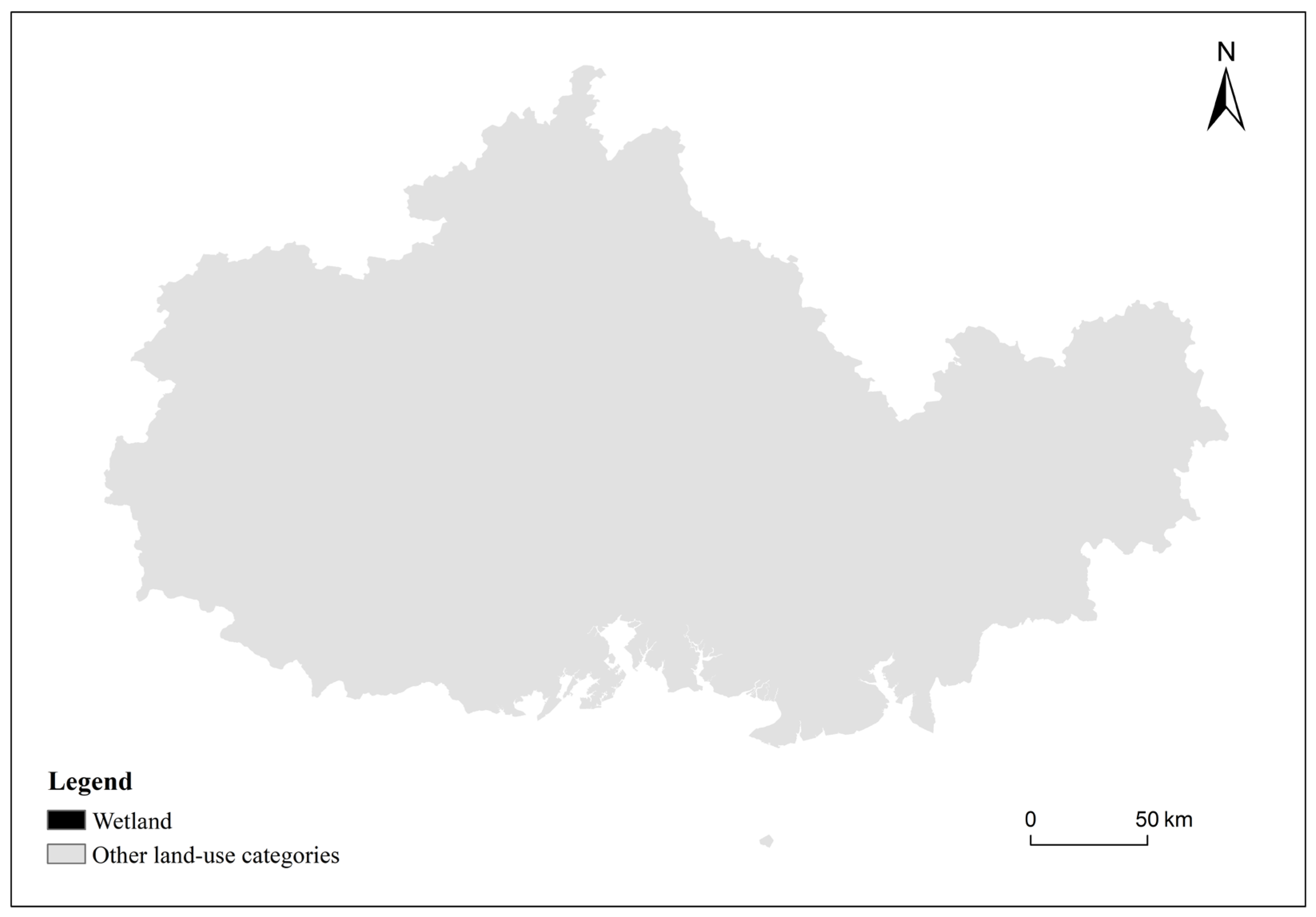
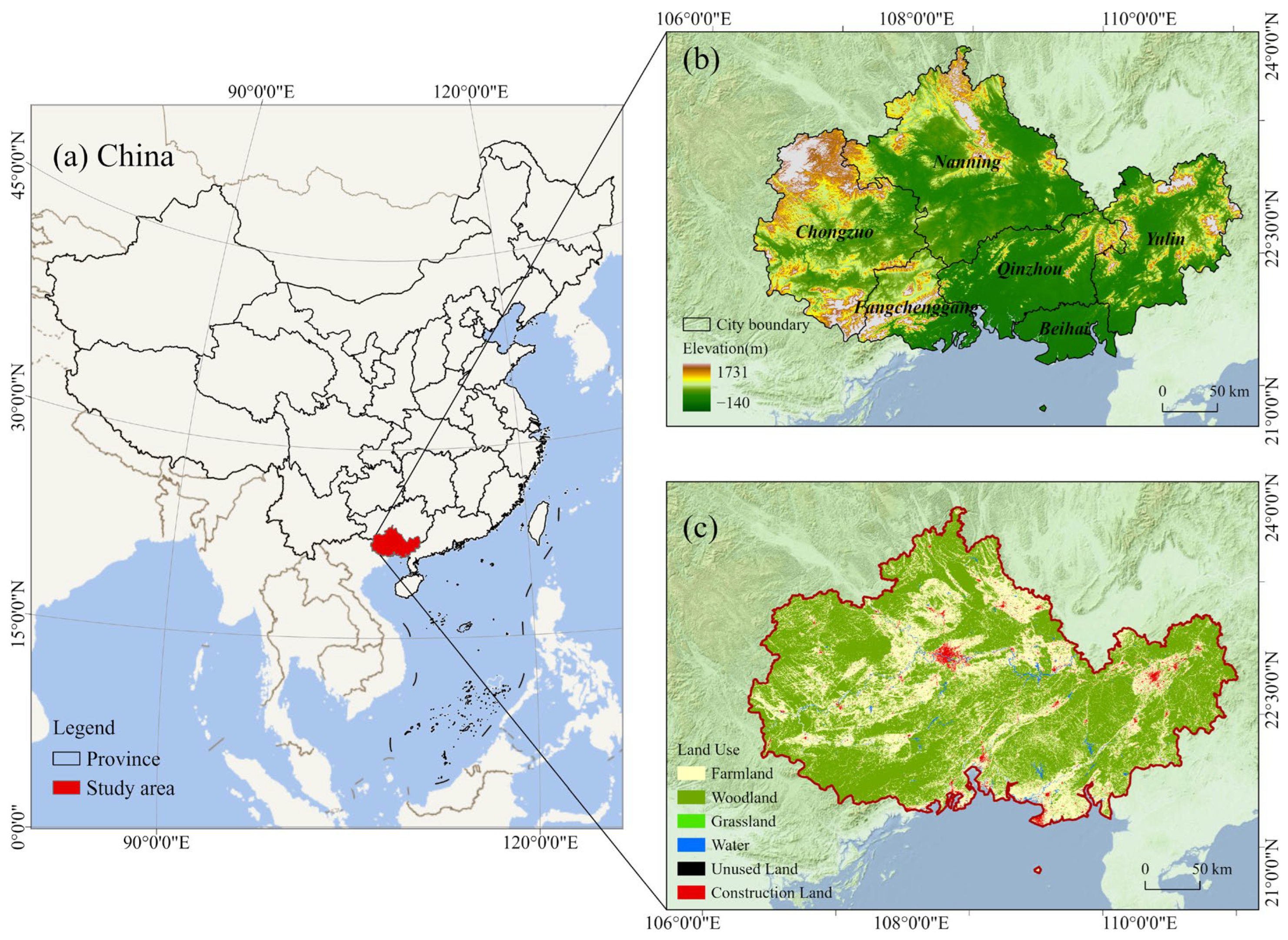
The study area is located in a typical karst–coastal transition zone in southern China, encompassing six prefecture-level cities in Guangxi, namely Nanning, Qinzhou, Beihai, Fangchenggang, Chongzuo, and Yulin (Figure 1). As a distinctive land–sea interactive ecological unit, this region constitutes a critical maritime hub of the New Western Land–Sea Corridor. Adjacent to the Indochina Peninsula, the study area possesses significant geographical advantages [21]. The region experiences a subtropical monsoon climate with abundant hydrothermal resources. The mean annual temperature is approximately 23 °C, and precipitation is ample throughout the year. The synchronous occurrence of precipitation and heat favors forest growth, endowing the native vegetation of this region with substantial carbon-stock accumulation potential [22]. The karst–coastal transition zone exhibits pronounced spatial heterogeneity in geomorphology. The northwestern part of the study area (covering Chongzuo and the northern part of Fangchenggang) consists predominantly of continuous karst mountain ranges; these areas have thin soil layers and low ecological resistance to disturbance, and are mainly covered by natural woodland, constituting the region’s core carbon-stock retention space. In contrast, the coastal areas of Beihai, Qinzhou, and Fangchenggang in the south belong to flat alluvial river plains; these coastal zones concentrate urban construction and port industries, accompanied by the rapid expansion of construction land. This study area is characterized by a fragile karst ecological base and high-intensity coastal human activities, making it an ideal study area for exploring the evolution patterns of carbon storage and the mechanisms behind land-use-change-attributable carbon-stock variations in the karst–coastal transition zone [23].

2.2. Research Data

All datasets were uniformly projected to the CGCS2000 geodetic coordinate system. The original land-use and carbon-stock datasets were 30 m resolution, while socioeconomic and climate predictors were native 1000 m resolution. To avoid artificial spatial details and spuriously low statistical significance caused by up-sampling coarse datasets to fine grids, all raster datasets for driver analysis, regression and LISA spatial autocorrelation were aggregated to a uniform spatial resolution of 1000 m. Data preprocessing, including clipping, mosaicking, and reclassification, was performed in ArcGIS Pro (v.3.5). Detailed sources for all datasets are listed in

Table 1. Data sources.

Data	Year	Spatial Resolution/Scale	Source
Administrative boundary data	2025	1:250,000	National Geospatial Information Public Service Platform (https://www.tianditu.gov.cn/)
Soil type data	2020	1000 m	Resources and Environmental Science Data Platform, Chinese Academy of Sciences (https://www.resdc.cn)
Population data	2020	1000 m	Resources and Environmental Science Data Platform, Chinese Academy of Sciences (https://www.resdc.cn)
GDP data	2020	1000 m	Resources and Environmental Science Data Platform, Chinese Academy of Sciences (https://www.resdc.cn)
Precipitation data	2024	1000 m	National Tibetan Plateau Data Center (https://data.tpdc.ac.cn)
Temperature data	2024	1000 m	National Tibetan Plateau Data Center (https://data.tpdc.ac.cn)
Vegetation coverage data	2024	1000 m	National Tibetan Plateau Data Center (https://data.tpdc.ac.cn)
Vector boundary of nature reserves in China	2024	1:1,000,000	Zenodo (https://zenodo.org)
Land use data	2000/2005/2010/2015/2020/2025	30 m	Zenodo (https://zenodo.org)
Road data	2020	1:1,000,000	OpenStreetMap (https://www.openstreetmap.org)
Water system data	2020	1:1,000,000	OpenStreetMap (https://www.openstreetmap.org)
Digital Elevation Model (DEM) data	2024	30 m	Geospatial Data Cloud (https://www.gscloud.cn)
Nighttime light data	2024	1000 m	Harvard Dataverse (https://dataverse.harvard.edu)

.

In terms of temporal matching, land-use-change-attributable carbon-stock variations were calculated for the period 2000–2025 using multi-temporal land-use datasets. This study primarily focuses on exploring the spatial coupling relationships between driving factors and carbon-stock variation patterns, rather than characterizing fine-scale year-by-year temporal dynamics. For the categorical soil-type variable, dummy variable encoding and standardization were performed prior to collinearity diagnosis and multiple linear regression, ensuring the suitability of this variable for VIF calculation and regression modeling. The 2025 land-use raster data (30 m resolution) were derived directly from the original CLCD dataset developed by Wuhan University, with no additional reconstruction or correction beyond unified reclassification. During preprocessing, the original wetland category was merged into the open water body class. This treatment was implemented because wetland pixels are extremely sparse and spatially fragmented across the study area; an independent wetland class with insufficient samples would cause unstable parameter estimation and unreliable simulation results in the PLUS model. Therefore, this study focuses exclusively on terrestrial carbon-stock variations dominated by typical land-use conversions and does not independently discuss wetland blue-carbon processes. Detailed data sources are listed in Table 1. The uniformly reclassified land-use dataset was directly adopted as the baseline input for PLUS model calibration and multi-scenario simulation.

2.3. Research Methods

2.3.1. Carbon Storage and Land-Use Carbon Emission Accounting Based on the InVEST Model

Carbon cycling is driven by terrestrial ecosystems. Terrestrial ecosystems absorb carbon dioxide from the atmosphere and further regulate the global climate system. The carbon storage and sequestration module embedded in the InVEST model requires carbon density parameters corresponding to each land use type; this module can calculate the total carbon storage within the study area [24]. The calculation formulas are shown in Equations (1) and (2).

$$C_i=C_{above}+C_{below}+C_{soil}+C_{dead}$$

(1)

$$C_{total}={\displaystyle \sum _{i=1}^n{A}_i{C}_i}$$

(2)

where C_i represents the carbon density of each land use type (t/hm²). C_above is the aboveground carbon density (t/hm²). C_below is the belowground carbon density (t/hm²). C_soil is the soil carbon density (t/hm²). C_dead is the dead organic matter carbon density (t/hm²).

Giardina et al. [25] used long-term in situ global soil observation data. Their results showed that the decomposition rate of mineral soil organic carbon responded weakly to temperature gradients; compared with living vegetation, the spatial variability of the soil carbon pool was much less strongly influenced by hydrothermal conditions. Accordingly, a relatively small soil carbon density correction coefficient, K_S ≈ 1.00, was adopted in this study for fine calibration. The initial carbon density parameters used in this study were obtained from Zhang et al. [26]; we followed the carbon density correction formulas proposed in several previous studies [27,28,29,30]. Differences in annual average temperature and annual precipitation serve as the basis for implementing local correction. The comparison region encompasses Yunnan and Guizhou, both of which belong to similar karst landform areas. Additionally, we calculated the precipitation correction factor, the temperature correction factor for vegetation carbon density, and the integrated correction factor. The carbon density correction formula is expressed as follows:

$$C_{SP}=3.3968\times MAP+3996.1$$

(3)

$$C_{BP}=6.798\times e^{(0.0054\times MAP)}$$

(4)

$$C_{BT}=28\times MAP+398$$

(5)

$$K_{BP}={\displaystyle \frac{C_{BP}^1}{C_{BP}^2}}$$

(6)

$$K_{BT}={\displaystyle \frac{C_{BT}^1}{C_{BT}^2}}$$

(7)

$$K_B=K_{BP}{K}_{BT}$$

(8)

$$K_S={\displaystyle \frac{C_{SP}^1}{C_{SP}^2}}$$

(9)

The above equations were used to adjust aboveground and belowground biomass carbon density. Liu et al. [31] conducted field observations of carbon density in four typical ecosystems in the karst regions of southwestern China; their results revealed the distinct characteristics of litter and coarse woody debris in karst areas. Calcium-bearing mineral retention and the relatively low degradability of lignin jointly regulate the organic carbon content in litter. At the regional scale, temperature and precipitation gradients induced almost no pronounced spatial variation in litter organic carbon density. Consequently, parameters measured within the same subtropical karst region can be adopted directly, without local calibration based on meteorological factors. Accordingly, this study directly employed published field measurements of litter organic carbon density in the karst regions of southwestern China, without introducing additional climate correction coefficients. No additional climate correction coefficient is introduced. Ultimately, carbon density parameters suitable for the karst–coastal transition zone in southern China were obtained; specific values are listed in

Table 2. Carbon density parameters (t·hm⁻²).

Land Use Types	C_Above	C_Below	C_Soil	C_Dead
Farmland	55.89	10.81	0.50	104.10
Woodland	260.76	272.09	5.67	71.77
Grassland	12.73	47.74	0.50	69.80
Water	9.28	7.94	0.25	64.03
Unused Land	4.91	0.46	0.00	43.71
Construction Land	0.00	3.12	0.00	28.42

.

This study uses periodic changes in carbon-stock to characterize land-use-change-attributable carbon-stock variations across the region. An increase in carbon-stock between two time periods represents land-use-driven carbon-stock gains; it does not imply enhanced ecosystem-level atmospheric carbon sequestration. Conversely, a decrease in carbon-stock signifies carbon-stock losses induced by land-cover transitions and should not be interpreted as the region acting as an atmospheric carbon source. This study employed the zonal statistics tool in ArcGIS to conduct refined statistical and time-series analyses of carbon-stock for different land-cover types and for the whole study area.

2.3.2. Land Use Transition Matrix

Land use transition matrices have been widely applied in related studies. This tool can reflect the extent and direction of conversions among different land cover types [32]; this method provides an important tool for clarifying the details of land use evolution and for conducting dynamic monitoring. The matrix can quantify the scale of mutual conversions among different land types over a specific period [33].

$$S_{ij}=\left[\begin{array}{cccc}{S}_{11}& S_{12}& \cdots & S_{1n}\\ S_{21}& S_{22}& \cdots & S_{2n}\\ ⋮& ⋮& & ⋮\\ S_{n1}& S_{n2}& \cdots & S_{nn}\end{array}\right]$$

(10)

where S_ij refers to the area of conversion from land use type i to land use type j throughout the study period. The symbol “n” stands for the total number of land-use types. “i” represents land types in the initial stage. The symbol “j” corresponds to land types of the final stage. The row vectors in the matrix correspond to the outward transformation directions and transformation areas of each land type; the column vectors reflect the input sources and transformation areas of each land type. Diagonal elements S_ii of the matrix denote land areas with no land use transformation. The original land use status of these lands remained unchanged throughout the study period.

2.3.3. Multicollinearity Test

The drivers of land-use-change-attributable carbon-stock variation involve multidimensional factors, including topographic, ecological, and socioeconomic conditions. These variables are highly susceptible to multicollinearity, which may lead to biased estimates of regression coefficients and distort the interpretation of driving mechanisms. Therefore, collinearity screening is required before conducting spatial statistical analysis and model analysis [34].

This study comprehensively considers the karst geomorphology, ecological environment, and socioeconomic characteristics of the study area. Twelve core driving factors are selected from four major dimensions. The four dimensions are terrain, ecological environment, socioeconomic status, and location conditions. Elevation, slope, vegetation coverage, and soil type constitute the specific influencing factors; mean annual temperature and mean annual precipitation are also included among these influencing factors. Other indicators include population density, GDP density, and nighttime light intensity; distance to roads, distance to water systems, and distance to nature reserves constitute the final three influencing factors.

Comprehensive diagnostics were performed using SPSS (v.26.0) statistical software. The test employed three indicators: the Pearson correlation coefficient, the variance inflation factor (VIF), and the tolerance value. Two widely accepted thresholds were used to identify severe multicollinearity: an absolute pairwise correlation coefficient |r| > 0.7 and a VIF ≥ 10. Variables exceeding these thresholds should be removed and the test rerun [35]. The results of the present study met the relevant criteria: the absolute correlation coefficients for all selected driving factors were below 0.7, and the VIF values for all factors were less than 3. These results indicate that only very weak linear correlations exist among the variables, with no risk of multicollinearity. In summary, all selected driving factors were retained for the subsequent bivariate local spatial autocorrelation analysis.

2.3.4. Spatial Autocorrelation Analysis

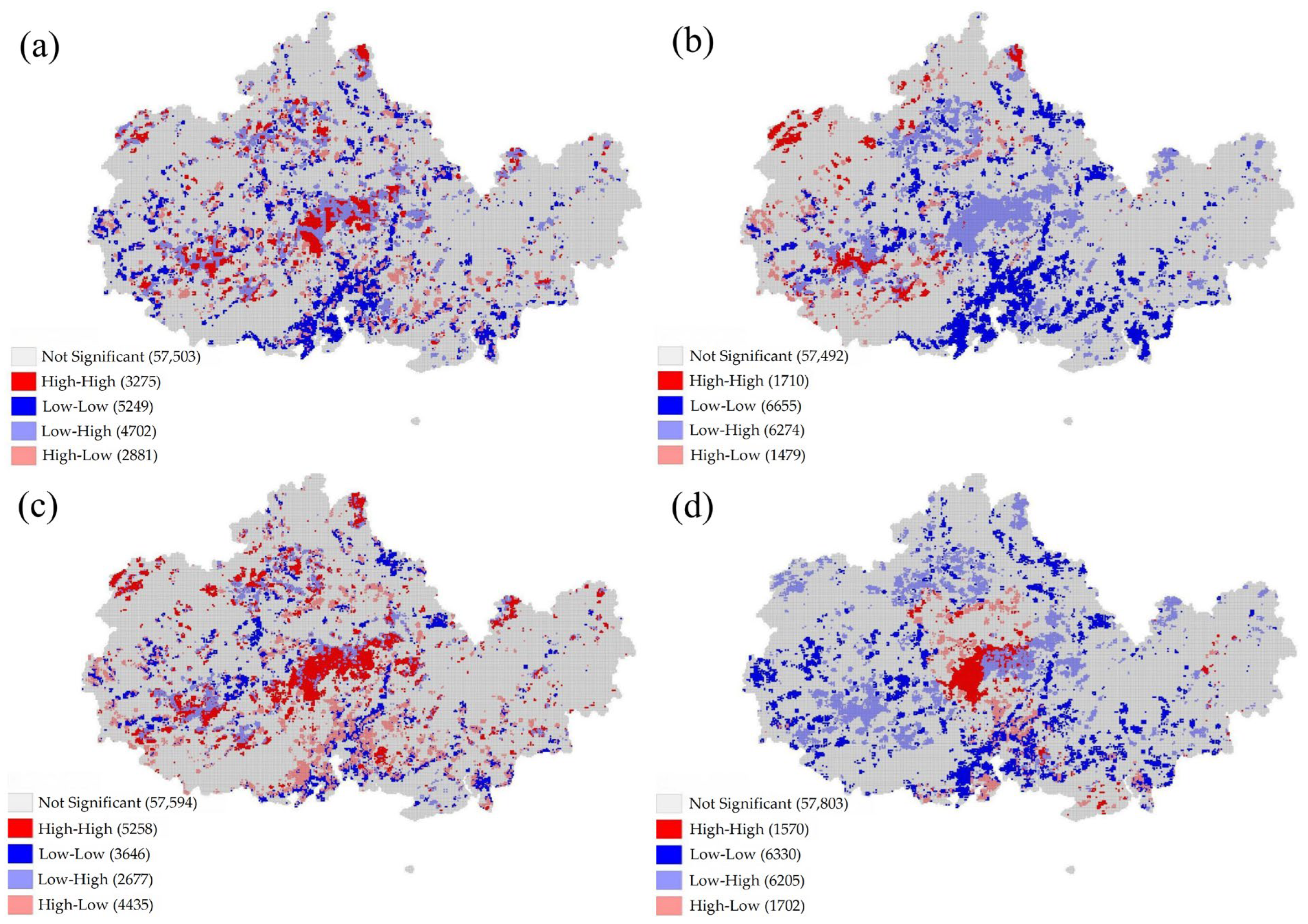
After preprocessing for multicollinearity, two categories of bivariate spatial autocorrelation statistics were applied in this study, namely global bivariate Moran’s I and local bivariate LISA. The global bivariate Moran’s I was adopted to quantify the overall spatial correlation between land-use-change-attributable carbon-stock variations and each driving factor across the whole study area. The local bivariate LISA was further used to detect location-specific spatial clustering patterns and regional disparities at the geospatial scale. Traditional statistical regression methods can only identify the global quantitative relationships between driving factors and land-use-change-attributable carbon-stock variations, and cannot capture spatial clustering patterns or regional differences at the geospatial scale. The study area encompasses diverse topography and land-use types, including karst mountainous areas, coastal plains, and urban built-up areas; both land-use-change-attributable carbon-stock variations and their driving factors exhibit pronounced spatial heterogeneity. In this study, GeoDa software (version 1.22.0.20) was employed to implement bivariate spatial autocorrelation analysis, aiming to reveal the spatial association patterns, clustering characteristics, and regional differences between the distribution of land-use-change-attributable carbon-stock variations and each driving factor [36].

The core indicator adopted to characterize global spatial autocorrelation is the global Moran’s I index. The corresponding formula is listed as follows:

$$I_a={\displaystyle \frac{n{\displaystyle {\sum }_{b=1}^n}{W}_{ab}{Z}_a{Z}_b}{{\displaystyle {\sum }_{a=1}^n}{Z}_a^2}}$$

(11)

where I_a stands for the local spatial autocorrelation index of spatial unit a, while n represents the overall number of spatial units across the whole study area. W_ab stands for the spatial weight matrix. This study adopts a first-order rook adjacency matrix to construct spatial association rules, defining spatial units that share an edge as adjacent units. This setting conforms to the spatial interaction characteristics of regional geographic units [37]. Z_a and Z_b are standardized attribute values of spatial unit a and neighboring unit b, respectively.

The local bivariate LISA statistic is defined as Equation (12):

$$L_i=Z_i{\displaystyle \sum _j{W}_{ij}{Z}_j}$$

(12)

where L_i is the local bivariate LISA value for spatial unit i; Z_i and Z_j are standardized attribute values; and W_ij refers to elements of the row-standardized spatial weight matrix.

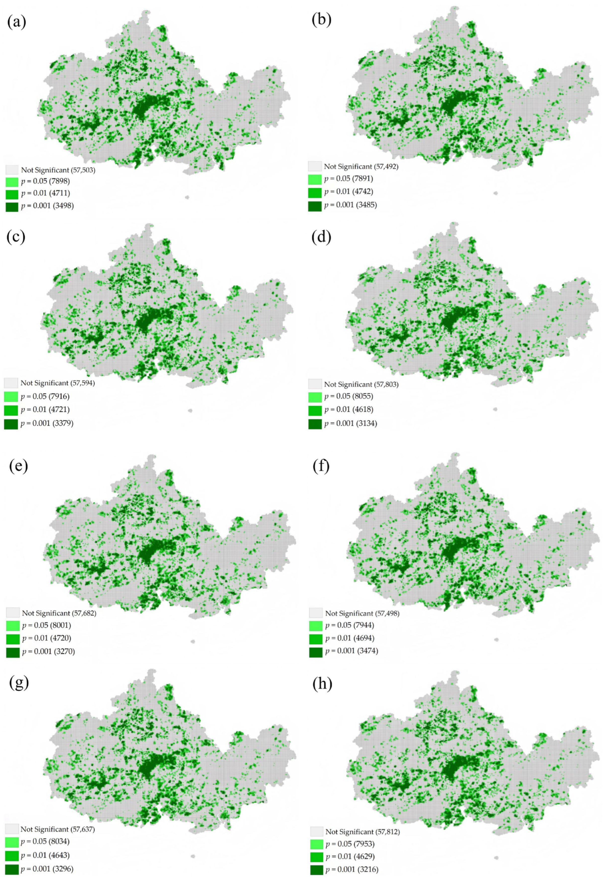
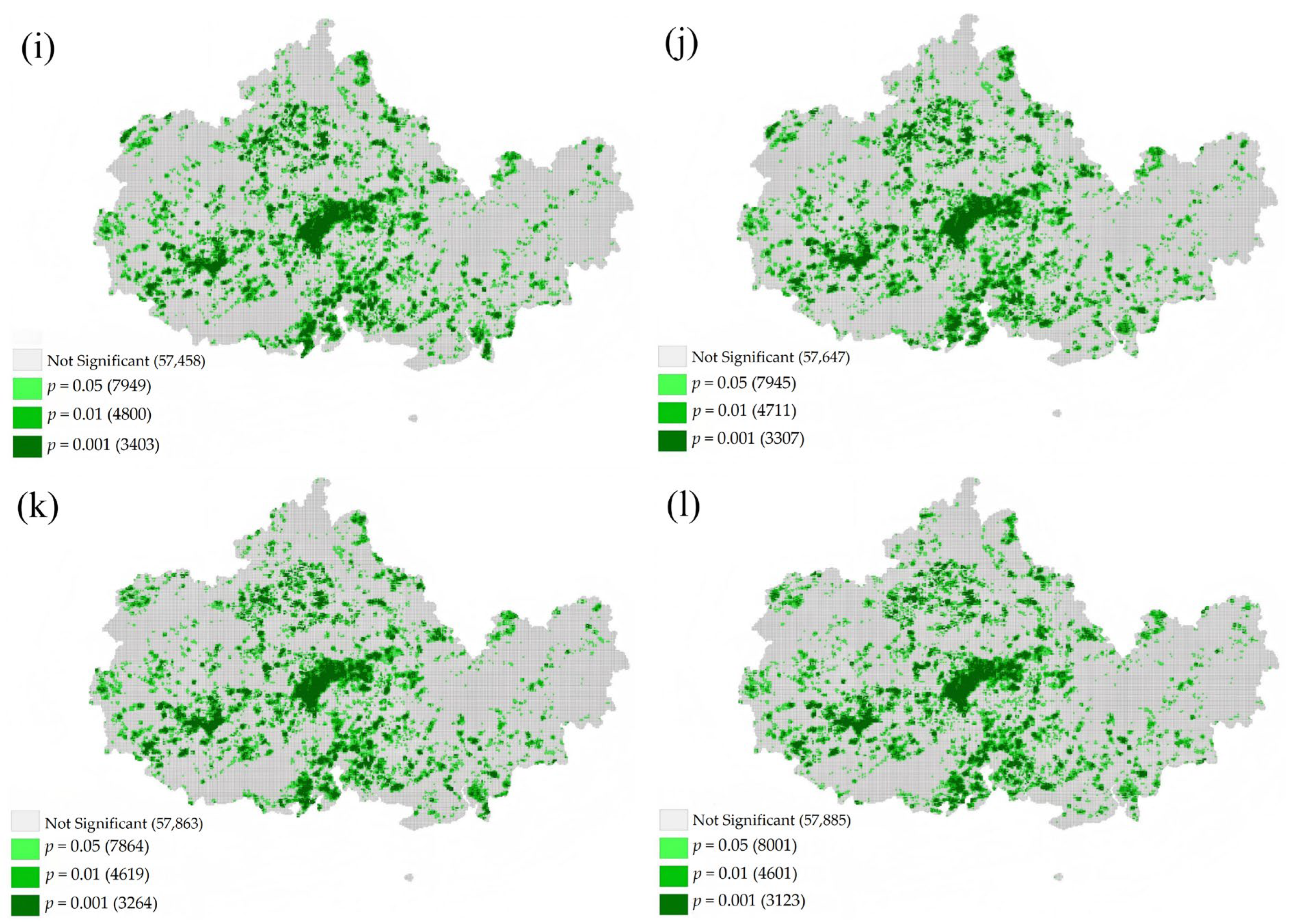
In the computation, Monte-Carlo simulation was used for the significance test; the number of simulations was set to 999, and the significance level was p = 0.05 [38]. For local LISA results, false-discovery-rate (FDR) correction was implemented to mitigate multiple-testing bias across massive spatial units. After FDR adjustment, all spatial units were classified into five types of spatial association patterns: High-High agglomeration (H-H), High-Low agglomeration (H-L), Low-High agglomeration (L-H), Low-Low agglomeration (L-L), and areas without significant spatial correlation.

2.3.5. Multiple Linear Regression Analysis of Driving Factors

We adopted forced-entry multiple linear regression to quantify the driving effects of explanatory variables on grid-scale land-use-change-attributable carbon-stock variations. The dependent variable was grid-level carbon-stock changes induced by land-use transitions. The spatial analysis unit was 1-km sampling grids across the entire study area, with a total sample size of 736,010. The regression analysis targeted the 2000–2025 study period. All twelve theoretically pre-selected predictors were forced into the regression model using the enter method, without removing variables according to statistical significance. Variance inflation factor (VIF) was calculated for multicollinearity diagnosis. Bivariate Moran’s I was computed to detect spatial correlation between each predictor and carbon-stock-change. Model fitness was reported as R² = 0.020 and adjusted R² = 0.020. The Durbin-Watson statistic was 1.124, which suggests potential residual autocorrelation for this ordinary least-square regression. It should be emphasized that this global ordinary least-square regression is not constructed for high-precision prediction of carbon-stock change. Given the huge sample volume of grid-based observations and strong spatial heterogeneity across the karst-coastal transition zone, numerous unmeasured local stochastic disturbances also shape carbon-stock variation. Therefore, the low R-square value is expected for such grid-scale global regression. The primary purpose of this regression is to compare the relative magnitude of driving effects by interpreting standardized beta coefficients, rather than pursuing strong model predictive performance.

2.3.6. Multi-Scenario Simulation Based on the PLUS Model

This study uses the Patch-generating Land-use Simulation (PLUS) model to simulate the spatial evolution of land use. The model integrates the LEAS framework for mining land expansion probabilities and includes a cellular automata (CA) module based on the CARS (clustering-based automata with random seeds) strategy. The PLUS model can generate fragmented land patches that conform to real topography; compared with traditional land-use simulation models, it achieves higher spatial simulation accuracy [39]. PLUS adopts a dual-scale simulation framework that organically combines macro-level land demand forecasting with micro-level spatial allocation [40]. Its overall modeling workflow comprises four steps: expansion probability calculation, CARS-CA-based iterative simulation, multi-scenario constraint setting, and accuracy validation.

This study applied a random forest algorithm to calculate land expansion probabilities. By overlaying historical land use data from two time periods, raster samples containing information on land use type conversions were extracted. We incorporated topographic, ecological, socioeconomic, and locational driving factors selected through multicollinearity testing. The random forest algorithm was used to explore the conversion patterns of each land type and to calculate the development probability of each raster cell expanding into different land types [41]. The CARS patch-generation cellular automaton combines a conventional cellular automaton with patch generation and threshold attenuation mechanisms, and this framework constitutes the CARS module; based on neighborhood weights, adaptive driving coefficients, and patch thresholds, the module enables automatic patch generation for each land type [36].

Using the 2025 land use raster data as the baseline, the model was calibrated with a screened set of unified driving factors. Three simulation scenarios were designed to distinguish different low-carbon management strategies: steep-slope carbon sink enhancement, ecological buffer zone carbon sequestration, and intensive low-carbon urban development. By combining the historical land use conversion characteristics from 2000 to 2025, management constraints were represented by adjusting the conversion probabilities among land use types. Under the steep-slope carbon sink scenario, the probability of conversion from construction land to steep-slope woodland, grassland, and farmland decreased substantially; this measure effectively curbed ecological degradation and soil organic carbon loss in steep-slope areas. Under the ecological-buffer scenario, the conversion probabilities for forest restoration increased, and development activities within ecological corridors were restricted. In the intensive urban scenario, disorderly outward urban expansion is restrained, and infill development within existing construction land is encouraged. The low-carbon objectives of each scenario are realized at the source of land use conversion by adjusting conversion probabilities. In the steep-slope carbon sink scenario, the weights of topographic factors such as slope and elevation are increased, and stricter constraints are imposed on ecological protection in steep-slope areas. In the enhanced low-carbon urban development scenario, the weights of urban expansion drivers, including GDP and nighttime light intensity, are reduced; this measure aims to mitigate disorderly urban expansion driven by economic growth. In the ecological buffer zone carbon protection scenario, this study increases the weights of ecological indicators such as vegetation coverage and distance to water systems, giving priority to maintaining the spatial stability of ecological buffer zones. If the driving factors were subjected to additions or deletions, the variable systems among the models for different scenarios would become inconsistent, thereby hindering an objective comparison of land evolution processes under different management pathways. Therefore, scenario-oriented differentiation is achieved solely by targeted adjustment of the weights of individual factors, while the complete driving factor system remains unchanged across all simulation runs.

The land use raster data of 2025 were adopted as the baseline dataset for the simulation. The three-level driving factor sets were screened through the aforementioned multicollinearity test and spatial autocorrelation analysis. Subsequently, model parameter adjustment, model calibration, and accuracy verification were carried out in sequence. The main parameter settings are described as follows:

First, land use transition rules (

Table 3. Land use transition rules under four simulation scenarios.

Land use type	Natural Development Scenario
	Farmland	Woodland	Grassland	Water	Unused land	Construction land
Farmland	1	1	1	1	1	1
Woodland	1	1	1	0	1	1
Grassland	1	1	1	1	1	1
Water	0	0	0	1	0	0
Unused land	1	1	1	1	1	1
Construction land	1	1	1	0	1	1
Land use type	Steep-slope Carbon Sequestration Enhancement Scenario
	Farmland	Woodland	Grassland	Water	Unused land	Construction land
Farmland	1	1	1	0	0	0
Woodland	1	1	1	0	1	0
Grassland	1	1	1	1	1	0
Water	0	0	0	1	0	0
Unused land	1	1	1	1	1	0
Construction land	1	1	1	1	1	1
Land use type	Ecological Buffer Carbon Conservation Scenario
	Farmland	Woodland	Grassland	Water	Unused land	Construction land
Farmland	1	1	1	1	0	0
Woodland	1	1	1	1	1	0
Grassland	1	1	1	1	1	0
Water	0	0	0	1	0	0
Unused land	1	1	1	1	1	1
Construction land	1	1	0	1	1	1
Land use type	Intensive Low-carbon Urban Management Scenario
	Farmland	Woodland	Grassland	Water	Unused land	Construction land
Farmland	1	1	1	1	0	0
Woodland	1	1	1	1	1	0
Grassland	1	1	1	1	1	0
Water	0	0	0	1	0	0
Unused land	1	1	1	1	1	1
Construction land	1	1	1	1	1	1

Note: 1 means allowable conversion, and 0 means prohibited conversion.

). The permissible and restrictive transition rules established for various land types were determined based on the historical land use conversion characteristics from 2000 to 2025.

Second, neighborhood weights (

Table 4. Neighborhood weight parameters.

Land Use Type	Farmland	Woodland	Grassland	Water	Unused Land	Construction Land
Neighborhood weight	0.65	0.75	0.06	0.44	0.02	0.59

). This study defines neighborhood influence coefficients according to the spatial expansion characteristics of different land use types: ecological land use types have relatively weak neighborhood expansion capacity, whereas construction land exhibits strong neighborhood expansion capacity. Third, transition probability thresholds. Differentiated thresholds are set according to the influence intensity of driving factors; the land spatial transition probabilities corresponding to the dominant driving factors are moderately increased.

Before interpreting the subsequent simulation results, it is necessary to first clarify the key model assumptions and boundary condition constraints. First, the coupled PLUS-InVEST workflow adopted in this study quantifies only changes in the organic carbon pool driven by land use and land cover change, and does not incorporate anthropogenic fossil carbon emissions from the industrial and energy sectors. Second, the modeling framework does not account for inorganic carbon sequestration generated by carbonate weathering processes in karst areas. Third, rocky desertification is treated as static background information rather than as a dynamic evolution module; therefore, sustained carbon losses caused by progressive rocky desertification degradation cannot be simulated by this model. Fourth, the carbon density parameters used for carbon storage estimation were derived from published regional literature and corrected along temperature-precipitation gradients, but systematic, full-coverage in situ soil profile sampling was not conducted across the entire karst-coastal ecological transition zone. Therefore, the simulated outputs represent only carbon-stock variations driven by land-use transitions represent only carbon changes driven by land use transitions; all conclusions derived from these simulations should be interpreted within the boundary conditions specified above and do not constitute a comprehensive assessment of regional ecosystem carbon balance.

This study uses four indicators to validate model accuracy: the Kappa coefficient, overall simulation accuracy [42], producer’s accuracy, and user’s accuracy corresponding to each land use type. The year 2020 is set as the baseline year and 2025 as the end of the validation period. Land use data for 2020 are imported to simulate the reverse land use pattern in 2025; the observed land use data for 2025 are used to compare with and validate the simulation results.

The producer’s accuracies for each land use type are as follows: farmland 0.875, woodland 0.954, grassland 0.406, water area 0.965, unused land 0.238, and construction land 0.853. The user’s accuracies for each land use type are listed in the table below: farmland 0.904, woodland 0.938, grassland 0.199, water area 0.922, unused land 0.448, and construction land 0.849. For the four dominant land use types (woodland, water area, farmland, and construction land), both the producer’s accuracies and user’s accuracies exceed 0.85, indicating good consistency in the simulation results. The accuracies for grassland and unused land are relatively low, mainly due to the breakup of spatial patches and insufficient sample sizes.

The calibrated model yields an overall Kappa coefficient of 0.846 across the entire study area, with an overall simulation accuracy of 92.42% and a Figure of Merit (FoM) of 0.628 for land-use change simulation. All accuracy metrics in this section are calculated on a cell-by-cell basis at a 30 m spatial resolution. The extremely low user’s accuracy for grassland (0.199) and the low-to-moderate user’s accuracy for unused land (0.448) arise from their highly fragmented distribution within the karst–coastal ecological transition zone; during PLUS model simulation, these small and scattered grassland and unused land patches are readily misclassified into the surrounding dominant land-cover types. Although these minor land categories occupy only a small fraction of the whole study area and exert limited influence on the overall simulation performance of major land-use classes, such misclassification may still bring potential uncertainties to carbon-storage projections under multiple ecological management scenarios. Overall, the model satisfies the accuracy requirements for regional dynamic land-use simulation, and its outputs can be regarded as reliable for the purpose of this study.

Nevertheless, the simulation performance varied among land use categories, which introduces category-specific uncertainty into future carbon storage projections. Compared with woodland, farmland, construction land, and water bodies, both grassland and unused land exhibited markedly lower producer’s accuracy and user’s accuracy. This pattern arises from the landscape characteristics of the karst coastal ecological transition zone: grassland and unused land patches are mostly scattered and small, making them prone to misclassification into adjacent dominant land cover types in PLUS simulations. Because land use transitions involving grassland and unused land patches have been incorporated into our multi-scenario parameter settings, such simulation biases can propagate into the carbon storage projections for 2030 and 2035, producing deviations at the local pixel scale. Even so, two factors constrain the magnitude of this uncertainty at the regional scale. First, grassland and unused land account for only a small proportion of the total study area, and their absolute contribution to regional total carbon storage therefore remains limited. Second, the producer’s accuracy and the user’s accuracy of the four carbon-dominant land use classes (woodland, farmland, construction land, and water bodies) all exceed 0.85. The satisfactory simulation performance for these major land classes ensures the robustness of regional carbon storage trends and cross-scenario comparisons, which constitute the core outputs of this study.

3. Results

3.1. Temporal Evolution of Land Use and Carbon Balance from 2000 to 2025

3.1.1. Land Use Structure and Transition Characteristics

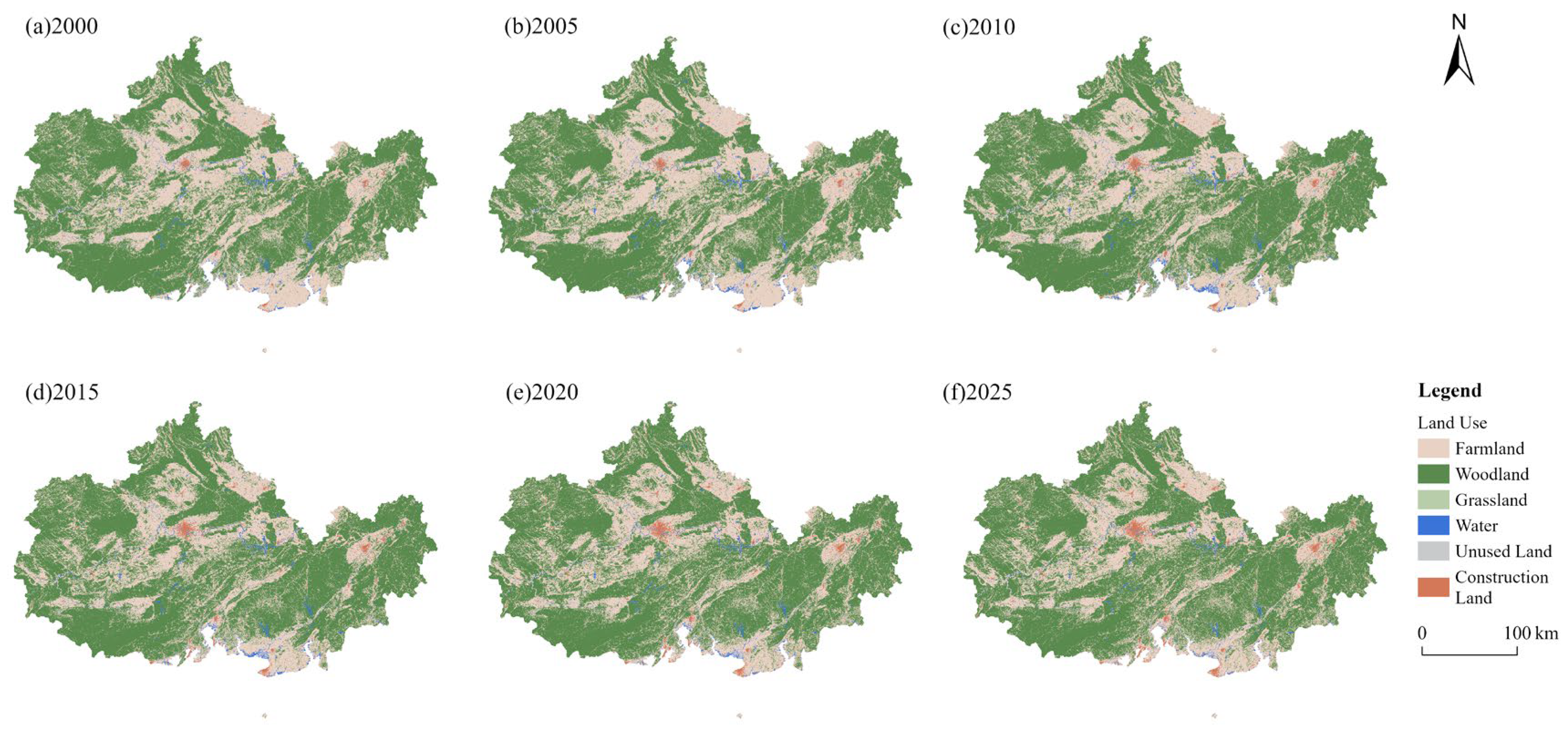
From 2000 to 2025, the land-use structure of the study area experienced continuous phased adjustment, with pronounced phased fluctuations observed for the six land-use types. As the dominant land-use type, woodland accounted for the largest proportion of the study area, with its share fluctuating between 58.95% and 63.38%. The structural variations of land-use types reflect land-use evolution under the joint influence of urbanization and ecological conservation. Farmland exhibited obvious phased fluctuations instead of a monotonic steady decline: its proportion increased from 37.01% in 2000 to 38.36% in 2005, dropped to the minimum value of 33.35% in 2015, and rebounded to 34.44% in 2025. Construction land maintained a sustained upward trend, rising from 0.93% in 2000 to 2.09% in 2025, which mirrors the obvious urban expansion process. Grassland and unused land maintained very low proportions across the whole period. Grassland showed non-monotonic fluctuation: it decreased from 0.075% in 2000 to 0.058% in 2010, rose slightly to 0.076% in 2015, and then declined sharply to 0.026% by 2025. Unused land remained at an extremely low level with minor oscillating changes. Water presented a trend of increasing first and then decreasing, reaching a peak proportion of 1.69% in 2010 and then falling to 1.20% in 2025. The overall land-use structural changes indicate that urban construction continuously brought pressure on farmland, woodland and other ecological land. Although woodland proportion is relatively high in karst mountainous regions, it is still confronted with disturbances from human development and settlement activities (Figure 2,

Table 5. Proportions of different land use types (%).

Time (Year)	Farmland	Woodland	Grassland	Water	Unused Land	Construction Land
2000	37.01	60.55	7.50 × 10−2	1.44	0.30 × 10−2	0.93
2005	38.36	58.95	6.20 × 10−2	1.57	0.20 × 10−2	1.06
2010	35.22	61.76	5.80 × 10−2	1.69	0.10 × 10−2	1.27
2015	33.35	63.38	7.60 × 10−2	1.62	0.10 × 10−2	1.58
2020	33.69	63.02	5.20 × 10−2	1.39	0.20 × 10−2	1.85
2025	34.44	62.24	2.60 × 10−2	1.20	0.40 × 10−2	2.09

).

Spatially, construction land exhibited the most remarkable changes, with its area achieving steady growth across the 25-year period. The hotspots of construction land expansion show obvious spatial agglomeration characteristics. In inland zones, construction land expands outward, centered on the two major urban centers of Nanning and Yulin. In coastal zones, it presents a belt-shaped expansion pattern along shorelines, port terminals and major roads of Qinzhou, Beihai, and Fangchenggang. Newly-added construction land is mainly composed of port-associated industrial land and urban residential land. By contrast, grassland, water, and unused land keep relatively stable spatial distribution patterns at the regional scale, despite obvious area fluctuations over time. The conversion magnitude of these three land-use types is limited, and their contributions to the overall adjustment of regional land-use structure are comparatively weak.

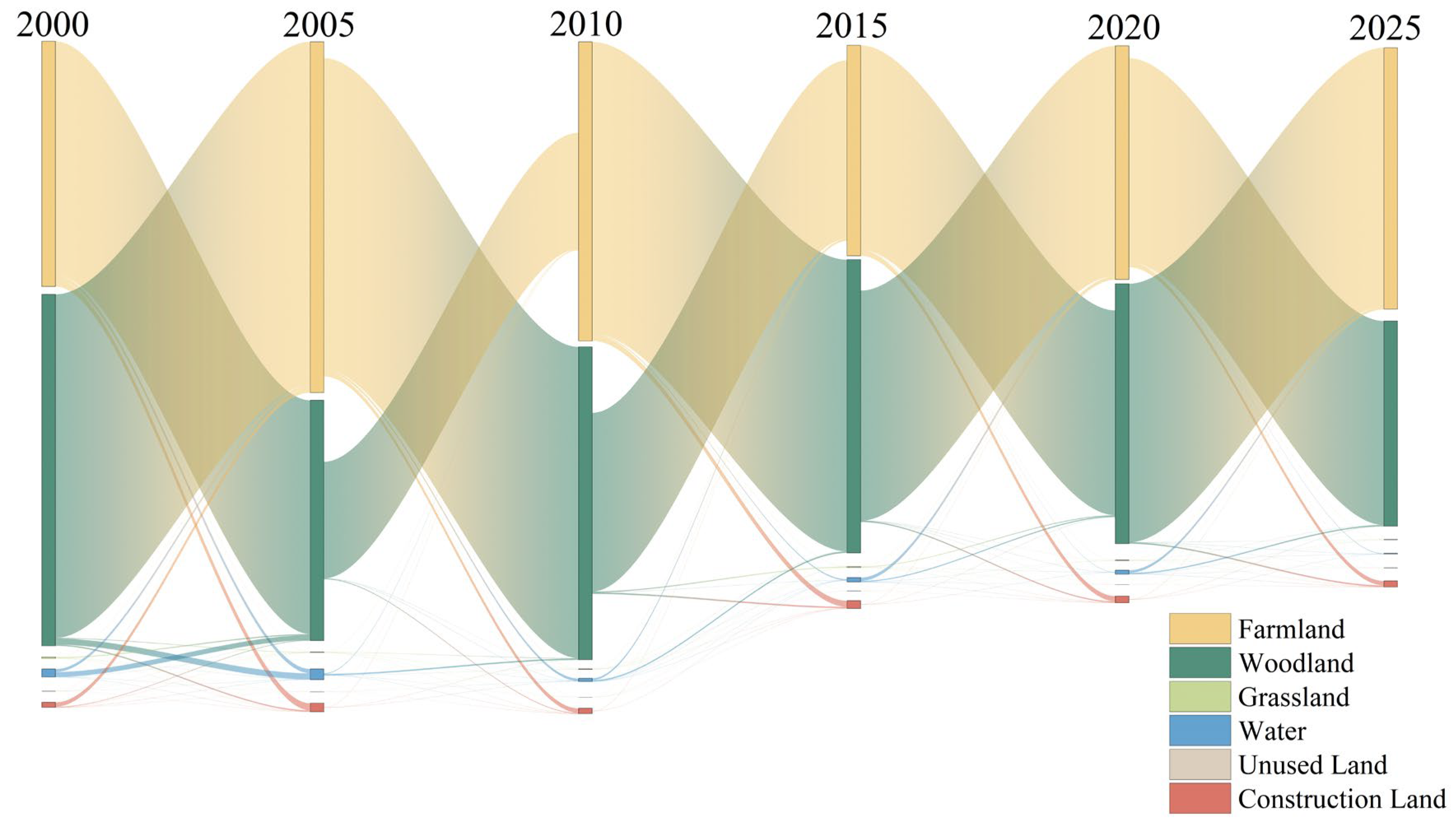
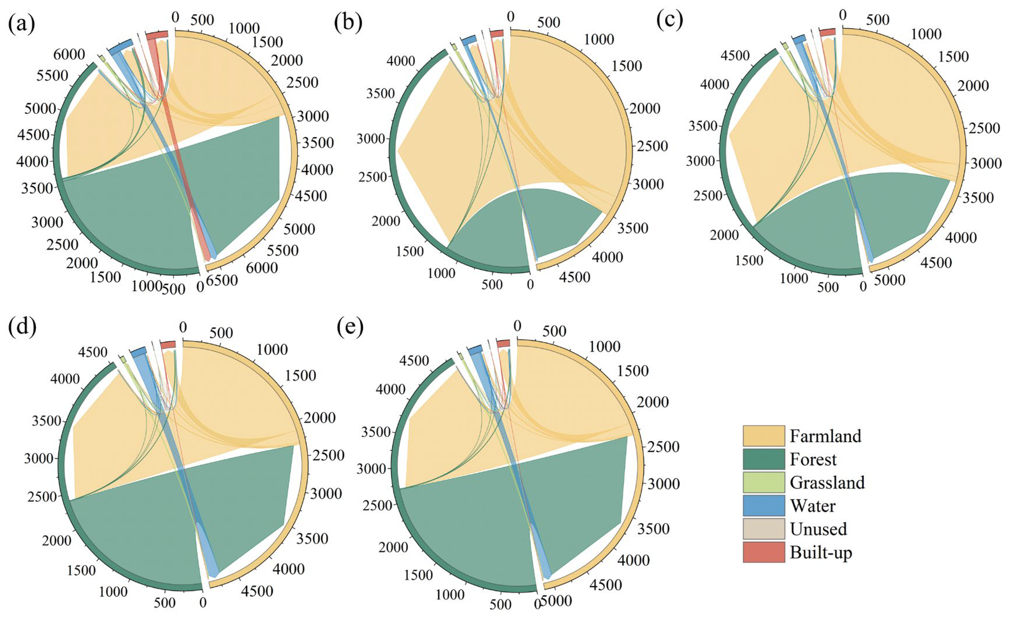
The land-use transfer matrices for the five periods indicate that, throughout the study period, the conversion of farmland and woodland to construction land was dominant and constituted the main driver of regional land-use structural change (Figure 3). Across different periods, land-use conversion was most active during 2010–2015 and 2015–2020. During these two intervals, the construction of the New International Land–Sea Trade Corridor accelerated, coastal port industries developed rapidly, and urbanization advanced markedly faster. Large contiguous tracts of woodland, high-quality paddy fields and dryland were expropriated and converted into industrial and mining land, urban construction land, and transportation land.

Small-scale reverse ecological transitions were also detected within the study area. Specifically, scattered degraded unused land, abandoned farmland on steep slopes, and dilapidated idle land were converted into woodland and grassland. Such ecological restoration transitions were mainly concentrated in remote karst mountainous regions, such as Chongzuo and northern Fangchenggang, which directly reflects the implementation effects of local natural restoration and rocky desertification control projects. Nevertheless, in terms of total converted area, the land gained via ecological restoration was substantially smaller than the area of ecological land occupied by construction land. Natural restoration alone cannot reverse the overall trend of land conversion toward non-agricultural and non-ecological purposes. Mutual conversions among grassland, water, and unused land took place with low frequency and small areal magnitude, corresponding merely to localized adjustments instead of large-scale overall structural transformation.

3.1.2. Temporal Changes in Regional Carbon Balance

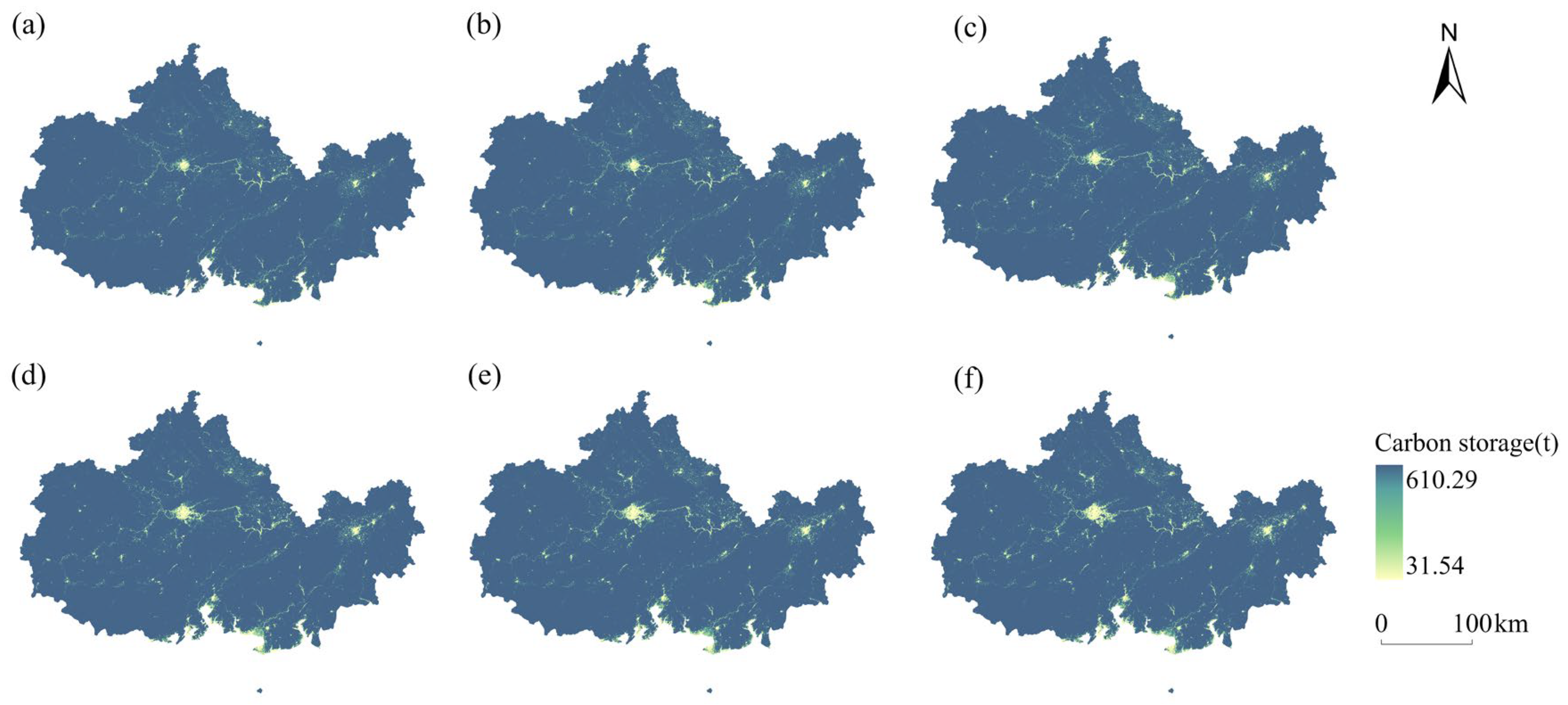
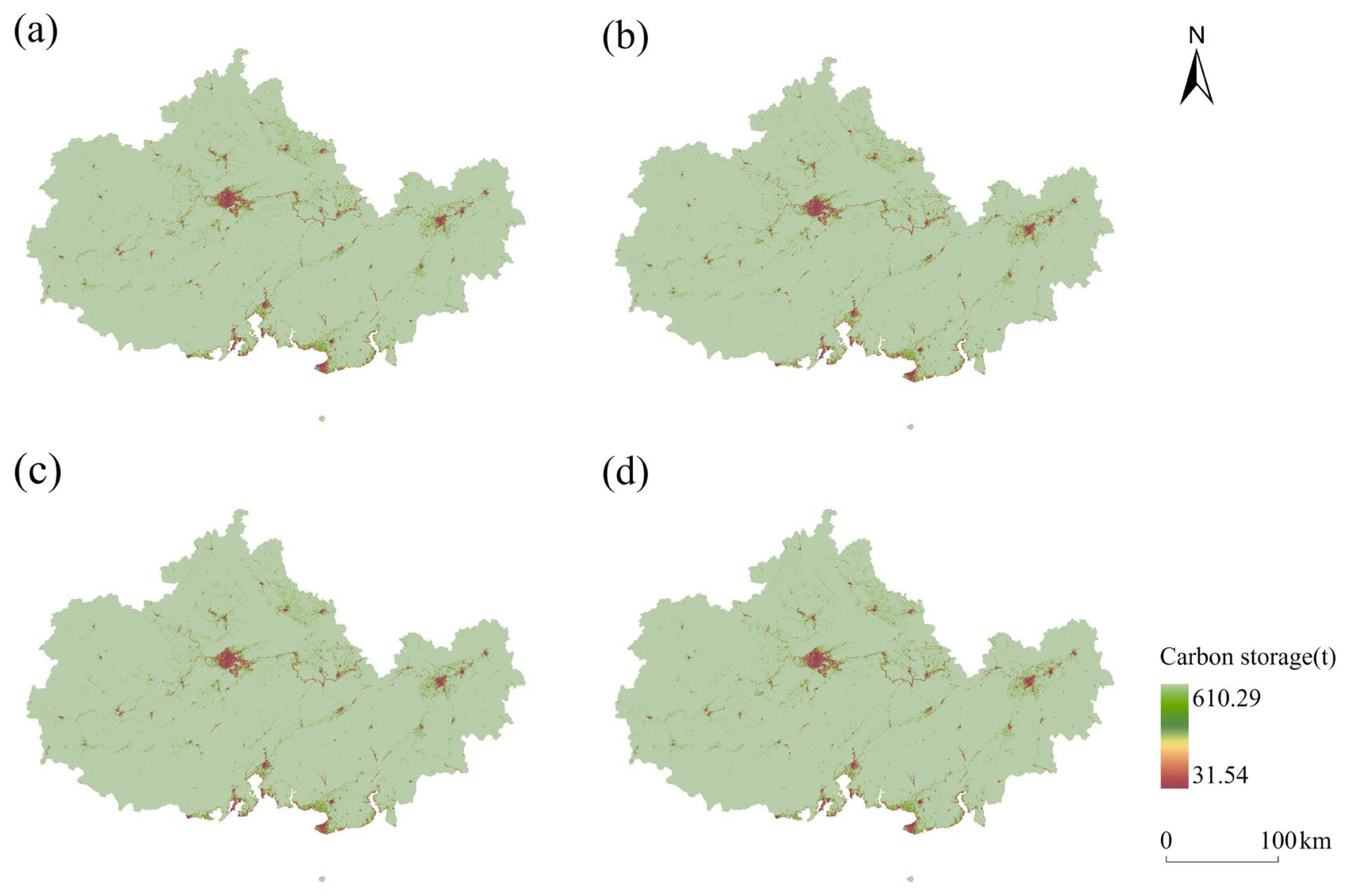
Carbon-stock values for each period were estimated using the InVEST model (Figure 4,

Table 6. Carbon storage of various land use types from 2000 to 2025 (million tons).

Time (Year)	Farmland	Woodland	Grassland	Water	Unused Land	Construction Land	Total	Total Change
2000	4572.19	26,650.82	7.04	84.82	0.11	21.11	31,336.10	/
2005	4739.97	25,974.00	5.84	92.14	0.06	24.08	30,809.09	−527.01
2010	4351.24	27,186.48	5.51	99.23	0.05	28.94	31,671.45	+862.36
2015	4119.96	27,899.60	7.14	94.98	0.04	35.93	32,157.65	+486.20
2020	4162.13	27,742.10	4.91	81.44	0.07	42.06	32,032.72	−124.93
2025	4255.14	27,395.76	2.43	70.54	0.15	47.60	31,771.62	−261.10

Note: Total Change is calculated as the total carbon-stock of the current year minus the total carbon-stock of the previous period. The year 2000 serves as the baseline year, and therefore no change value is provided for 2000.

). The total change between adjacent periods represents land-use-change-attributable carbon-stock variations across the region. Positive values indicate carbon-stock gains within the corresponding interval, whereas negative values indicate carbon-stock losses. From 2000 to 2025, regional carbon-stock showed obvious fluctuating characteristics: it decreased from 2000 to 2005, then increased continuously during 2005–2010 and 2010–2015, reaching its maximum value in 2015. After 2015, regional carbon-stock underwent continuous decline until 2025.

From 2000 to 2025, regional carbon-stock exhibited a fluctuating evolutionary trend characterized by three distinct phases. The first phase, spanning 2000–2005, witnessed a carbon-stock decrease of 527.01 million tonnes. During this period, woodland area in the northwestern karst mountainous region declined, and the carbon-stock losses induced by woodland reduction were not fully offset by the moderate expansion of farmland, resulting in an overall regional carbon-stock decline. The second phase, covering 2005–2015, saw continuous carbon-stock growth, with increases of 862.36 million tonnes during 2005–2010 and 486.20 million tonnes during 2010–2015. A series of ecological engineering projects—including rocky desertification control, the Grain for Green Program, and public welfare woodland conservation—were advanced continuously throughout this phase. Woodland area in the northwestern karst mountainous region recovered progressively, ecosystem integrity gradually improved, and land-use-change-attributable carbon-stock gains steadily rose. Although initial urban expansion occurred during this period, the extent of ecological land occupied by construction land remained limited, and the carbon-stock gains generated by ecological restoration were sufficient to offset the carbon-stock losses caused by land-use conversion. Regional carbon-stock reached its maximum value of 32,157.65 million tonnes in 2015. The third phase, spanning 2015–2025, exhibited a continuous declining trend, with decreases of 124.93 million tonnes during 2015–2020 and 261.10 million tonnes during 2020–2025. As urbanization and port-oriented industrial development intensified significantly, land types with high carbon density, such as farmland and woodland were occupied on a large scale. The regional core carbon pool sustained progressive degradation, and areas featuring land-use-change-attributable carbon-stock losses continued to expand. Certain areas gradually shifted from zones of carbon-stock gains to zones dominated by carbon-stock losses, while the mismatch between carbon-stock gains and losses induced by land-use change became increasingly pronounced. In analyzing carbon-stock contributions across land types, woodland consistently accounted for more than 84% of the regional total carbon-stock throughout the study period, serving as the primary carbon pool of the study area. Changes in woodland area directly determined the overall trend of regional land-use-change-attributable carbon-stock variations. Farmland ranked second in carbon-stock contribution; its area reduction directly led to losses in the agricultural carbon pool, constituting the secondary source of regional carbon-stock losses. Construction land exhibited the lowest carbon density among all land types; the continual expansion of this land type persistently reduced the regional carbon-stock retention capacity. Grassland, water, and unused land accounted for extremely low shares of regional carbon-stock; fluctuations in the area of these land types had a negligible impact on land-use-change-attributable carbon-stock variations. The integrated time-series data indicate that changes in land-use structure are highly coupled with the evolution of regional carbon-stock. Therefore, land-use system transformation is the core factor shaping carbon-stock patterns within the karst–coastal transition zone of southern China.

3.1.3. Spatial Differentiation Characteristics of Carbon Balance

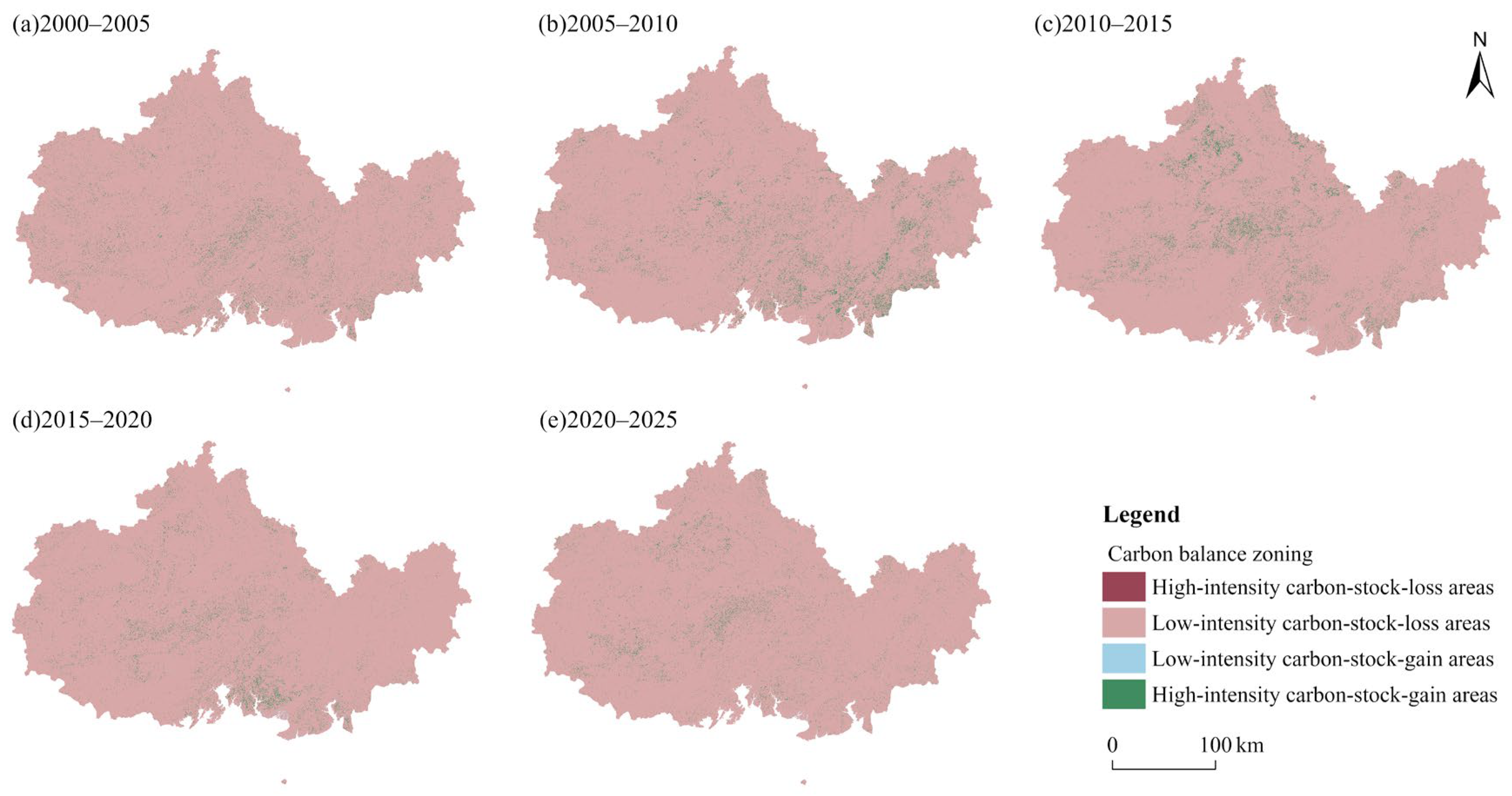
In this study, the natural breaks classification method in ArcGIS was applied to gridded carbon-stock variation data induced by land-use change for each period (Figure 5). The classification thresholds are defined strictly as follows: −578.75 t to −442.57 t for high-intensity carbon-stock-loss areas; −442.57 t to 0 t (exclusive of zero value) for low-intensity carbon-stock-loss areas; 0 t to 138.45 t (exclusive of zero value) for low-intensity carbon-stock-gain areas; and 138.45 t to 578.75 t for high-intensity carbon-stock-gain areas. Pixels with an exact zero value represent locations with no net carbon-stock change; these pixels are neither carbon sources nor carbon sinks and are not assigned to any of the four visualized categories in Figure 5. All grid-level carbon-stock-variation values correspond to total carbon mass (tonnes) per 30 m pixel. The results show that from 2000 to 2025, land-use-driven carbon-stock variations across the study region presented obvious concentric-zonal spatial differentiation, and such a spatial pattern kept evolving over time.

High-intensity carbon-stock-gain zones constitute the regional core carbon pool, concentrated in the administrative area of Chongzuo in the northwestern part of the study area and the karst mountainous region of northern Fangchenggang. These areas are characterized by steep topography, thin soil layers, and poor transportation accessibility, which makes large-scale development and construction difficult under low-intensity human disturbance. Contiguous natural woodlands are distributed across the region, with intact vegetation community structure; this ecosystem possesses exceptionally strong carbon-stock-accumulation potential, constituting the most stable carbon-stock-retention space within the entire study area. Low-intensity carbon-stock-gain zones ring the periphery of high-intensity carbon sink zones, while also being scattered along small inland water systems and within and around protected areas at various levels. These areas have a high proportion of ecological land, and human development activities are constrained by ecological principles. Their carbon pools remain relatively stable and can continuously maintain carbon-stock-gain performance, but their magnitude of carbon-stock increase is lower than that of the core karst mountainous areas. Low-intensity carbon-stock-loss areas are mainly distributed in urban–rural transition zones, around township settlements, and on intermountain platforms with concentrated contiguous farmland. In these areas, farmland, woodland, and construction land are interwoven, and land-use systems undergo frequent changes. The increase and decrease in carbon storage maintains a dynamic balance, and the overall characteristic is relatively weak carbon-stock-loss magnitude. These areas serve as buffer transition zones between carbon-stock-gain areas and high-intensity carbon-stock-loss areas. High-intensity carbon-stock-loss areas are continuously distributed along the major transport corridors, shorelines, and urban centers of prefecture-level cities, forming multiple belt-like and large-scale high-carbon-stock-loss corridors. The urban core of Nanning, the urban area of Yulin, and the coastal ports and industrial parks along the Beibu Gulf have become the core hotspots of carbon-stock loss. In these areas, construction land is highly concentrated, while the original ecological land has undergone severe fragmentation. Carbon stock capacity has declined sharply, making these areas the primary sources of regional land-use-change-attributable carbon-stock losses. Spatial pattern analysis further indicated that areas characterized by severe and moderate carbon-stock degradation underwent continuous outward expansion throughout the 25-year period. These areas continuously encroached upon adjacent low-intensity carbon sink areas and progressively compressed carbon-stock-retention space. Only remote karst mountainous areas with complex topography and strict ecological conservation requirements have maintained intact high-intensity carbon sink areas. The spatial differentiation of land-use-change-attributable carbon-stock variations is highly consistent with the regional geomorphological patterns and the spatial layout of land use, which further indicates that land-use patterns dominate the spatial patterns of land-use-change-attributable carbon-stock variations.

3.1.4. Characteristics of Land Use Transitions and Their Coupling Relationships with Carbon Balance, 2000–2025

By integrating six periods (2000, 2005, 2010, 2015, 2020, and 2025) of 30 m land-use grid datasets with periodic carbon-stock results for each land-cover type simulated by the InVEST model, we defined the land-use-change-attributable carbon-stock variation of each spatial unit as the difference in carbon-stock between adjacent periods. Specifically, carbon-stock of the earlier period was subtracted from that of the later period; a negative value indicates a decrease in carbon-stock, representing carbon-stock loss, whereas a positive value indicates an increase in carbon-stock, representing carbon-stock gain.

Throughout the study region, the conversion of woodland and farmland to construction land was the primary cause of carbon stock reduction. As shown in the Sankey diagrams corresponding to each period in Figure 6, the flows representing the conversion of woodland and farmland to construction land consistently maintained the largest magnitude throughout the study period. The aboveground and belowground carbon densities of karst woodland were markedly higher than those of urban construction land, whereas coastal farmland harbored a rich surface soil organic carbon pool. The conversion of these two land categories with high carbon baselines to urban and industrial land resulted in substantial declines in carbon stocks, thereby producing persistent land-use-change-attributable carbon-stock losses across all stages. Since 2015, the construction of the New International Land-Sea Trade Corridor and the concentrated development of coastal industrial parks have accelerated. The carbon stock losses resulting from the conversion of coastal farmland to non-agricultural uses have continued to expand, becoming the major driver of regional mismatch between carbon-stock gains and losses. The conversion of karst woodland and steep-slope grassland to terraced farmland constitutes a distinctive carbon loss pathway in mountainous areas. During the 2000–2015 period, substantial carbon flows corresponding to the conversion of woodland and grassland to farmland can be observed, concentrated in the karst mountainous areas of Chongzuo and northern Fangchenggang. In the concentrated distribution areas with slopes greater than 15°, the soil layer is relatively thin. The reclamation of primary woodland and grassland for cultivation has exacerbated soil erosion and persistent organic carbon loss, leading to prolonged land-use-change-attributable carbon-stock losses in these regions. Since 2010, the region has fully implemented the “Grain for Green” program; the scale of such carbon-loss land-use systems has contracted markedly, effectively mitigating the mismatch between carbon-stock gains and losses in mountainous areas. The conversion of unused land to farmland constitutes a secondary source of carbon stock loss. When exposed karst bedrock, degraded rocky desertification land, and unused land are converted to farmland, the pre-existing carbon pools of low shrubs and grassland are eliminated, and surface soil carbon loss occurs under cultivation disturbance, which generates land-use-change-attributable carbon-stock losses. However, the inherent carbon stock of unused land is extremely low, corresponding to the narrow carbon loss flux intervals in the Sankey diagram; consequently, its contribution to the regional mismatch between carbon-stock gains and losses is negligible.

Based on the temporal variation characteristics of carbon-stock-change flows shown in Figure 6, the evolution of land-use-change-attributable carbon-stock variations across the region can be grouped into two distinct stages. The first stage corresponds to 2000–2010, featuring mixed carbon-stock gains and losses. During this period, steep-slope reclamation in karst mountain areas occurred alongside outward expansion of coastal towns. Large-area woodland and farmland were converted into construction land and sloping farmland, and the carbon-stock-change flows corresponding to these conversions kept rising, which aggravated regional carbon-stock losses. Nevertheless, ecological restoration practices also brought partial carbon-stock gains, so the overall regional carbon-stock still achieved a notable increase from 2005 to 2010. The second stage covers 2010–2025 with divergent carbon-stock evolution among sub-regions. The Grain for Green Program implemented in mountainous regions effectively mitigated carbon-stock losses induced by steep-slope cultivation. Nevertheless, port-driven coastal urban expansion persisted, and carbon-stock losses triggered by the conversion of farmland to non-farmland kept growing. The carbon-stock gains from mountain ecological restoration could no longer counterbalance the carbon-stock losses caused by urban-related land conversion. Consequently, the whole region suffered continuous net land-use-change-attributable carbon-stock losses after 2015.

3.2. Analysis of Driving Factors for Carbon Balance

3.2.1. Results of Multicollinearity Test

All twelve driving-factor variables were standardized prior to analysis and assessed for multicollinearity using the variance inflation factor (VIF). The VIF values for all predictors were lower than 3, far below the commonly adopted critical threshold of VIF = 10 for severe multicollinearity. Accordingly, severe multicollinearity was not detected among these explanatory variables (

Table 7. Results of bivariate spatial autocorrelation and collinearity test for driving factors.

Driving Factor	Bivariate Moran’s I	Spatial Significance (p)	Standardized Beta Coefficient (β)	Linear Significance (p)	VIF	Influence Direction
Distance to road	3.30 × 10−2	1.00 × 10−3	1.00 × 10−2	0.02	1.21	Positive
FVC	5.20 × 10−2	1.00 × 10−3	7.00 × 10−2	<0.001	1.86	Positive
DEM	7.50 × 10−2	1.00 × 10−3	12.50 × 10−2	<0.001	2.66	Positive
GDP	−2.10 × 10−2	1.00 × 10−3	0.60 × 10−2	0.19	1.60	Positive
Precipitation	−3.10 × 10−2	1.00 × 10−3	−2.70 × 10−2	<0.001	1.23	Negative
Slope	3.40 × 10−2	1.00 × 10−3	−10.90 × 10−2	<0.001	2.72	Negative
Population	−1.90 × 10−2	1.00 × 10−3	0.60 × 10−2	0.19	1.68	Positive
Distance to water system	5.80 × 10−2	1.00 × 10−3	3.00 × 10−2	<0.001	1.16	Positive
Soil	−6.90 × 10−2	1.00 × 10−3	−7.30 × 10−2	<0.001	1.14	Negative
Temperature	−1.20 × 10−2	1.00 × 10−3	2.60 × 10−2	<0.001	1.29	Positive
Nighttime light	−4.80 × 10−2	1.00 × 10−3	−0.60 × 10−2	0.23	1.63	Negative
Distance to nature reserve	3.90 × 10−2	1.00 × 10−3	4.50 × 10−2	<0.001	1.17	Positive

). All twelve pre-selected factors were therefore retained for the subsequent forced-entry multiple linear regression analysis.

The results of forced-entry multiple linear regression analysis indicated that factors from different dimensions exerted differential impacts on land-use-change-attributable carbon-stock variations. Topographic-ecological and climatic factors exhibited mixed coefficient signs. Elevation, vegetation coverage, distance to protected areas, distance to water bodies, distance to roads, and temperature yielded positive standardized Beta coefficients and contributed to maintaining regional carbon storage. By comparison, slope, soil, and precipitation showed negative Beta coefficients, constraining the retention of regional carbon storage. Socioeconomic factors showed mixed coefficient signs: GDP density and population density had positive standardized Beta coefficients, whereas nighttime-light intensity returned a negative coefficient. Several predictors achieved statistical significance at p < 0.05. Notably, although GDP density, population density, and nighttime-light intensity showed significant spatial correlations with carbon-stock variation from bivariate Moran’s I statistics, their regression coefficients became statistically non-significant in the multivariate model after controlling for other driving factors (p > 0.05).

3.2.2. Spatial Autocorrelation and Classification of Driving Factors

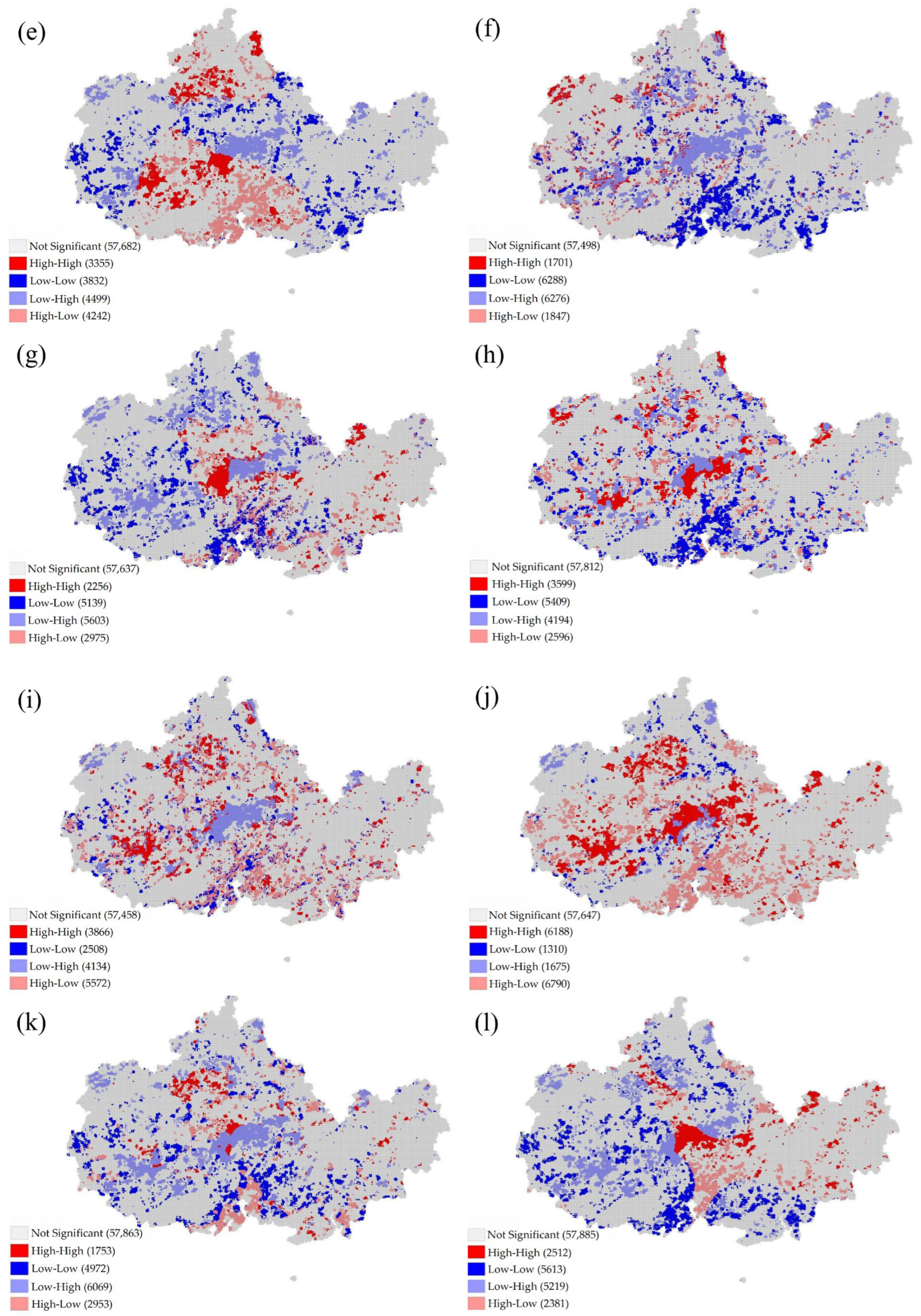
Based on the bivariate local LISA spatial autocorrelation analysis results, significant spatial clustering correlations exist between the 12 driving factors and land-use-change-attributable carbon-stock-variation, although the influence magnitude and spatial differentiation characteristics differ across driving factors (Figure 7). This study took the absolute values of standardized Beta coefficients as the primary basis for hierarchical classification, and adopted the natural attributes of each driving factor as well as the spatial association strength derived from bivariate local Moran’s I as auxiliary verification, to construct a three-level transmission-regulation hierarchical structure (Figure 8). Rather than adopting universally fixed statistical cutoff values, the thresholds of 0.10 and 0.03 were determined according to numerical gaps in the frequency distribution of standardized Beta coefficients for all 12 driving factors. These two breakpoints were further cross-validated against the outputs of bivariate local LISA-based Moran’s I spatial association analysis.

To test the robustness of this classification scheme, we further conducted sensitivity tests using two sets of adjacent alternative thresholds (see

Table A1. Sensitivity test of Beta-based driving-factor tier classification.

Scheme	Tier-1 (|β|≥)	Tier-2 (|β|)	Tier-3 (|β|≤)	Count of Tier-1 Factors	Count of Tier-2 Factors	Count of Tier-3 Factors
Baseline	0.10	0.03 < |β| < 0.10	0.03	2	3	7
Perturbation 1 (lower)	0.09	0.025 < |β| < 0.09	0.025	2	6	4
Perturbation 2 (higher)	0.11	0.035 < |β| < 0.11	0.035	1	4	7

Note: Absolute standardized Beta coefficients are derived from Table 7.

). When the thresholds were slightly lowered (0.09, 0.025), the two dominant topographic factors (DEM and slope) remained stably assigned to the first level, while only a few variables near the critical values shifted between the second and third levels. When the thresholds were slightly raised (0.11, 0.035), the slope factor moved from the first level to the second level, because its standardized Beta coefficient (β = 0.109) was close to the upper threshold. This indicates that the upper cutoff of 0.10 falls within a natural numerical gap between 0.073 and 0.109; the classification is more sensitive to upward adjustment of this threshold but remains robust against downward adjustment. Overall, this grouping scheme adequately captures the hierarchical mechanisms shaped by topographic context, ecological constraints, and human disturbance in the karst–coastal ecotone. The relevant classification thresholds, corresponding indicators, and underlying mechanisms are as follows:

Factors with |β| ≥ 0.10 were defined as “primary topography-dominated factors,” including elevation and slope. These factors had the highest local Moran’s I values and the strongest spatial autocorrelation, constituting the intrinsic baseline conditions that.

Factors satisfying the condition 0.03 < |β| < 0.10 were classified as “secondary ecological constraint factors,” encompassing four indicators: vegetation coverage, soil type, distance to water bodies, and distance to nature reserves; such factors function as ecological barriers. In regions with dense vegetation, riparian ecological zones, and nature reserves, ecosystems remain stable, and carbon pools exhibit strong resistance to disturbance, thereby effectively mitigating carbon loss induced by human development activities; however, once these ecological constraints are degraded, carbon stocks decline rapidly. These factors are key supporting elements for maintaining the spatial stability of local carbon-stock-gain performance. Factors with |β| ≤ 0.03 were classified as tertiary socioeconomic disturbance factors, including GDP density, population density, nighttime light intensity, and distance to roads. These factors shape the regional pattern of land-use-change-attributable carbon-stock variations represent anthropogenic disturbances: population agglomeration, economic growth, and the expansion of transportation networks directly drive the proliferation of construction land, encroaching upon ecological carbon pools such as woodland and farmland and disrupting the original carbon cycling balance of terrestrial ecosystems; they constitute the core drivers of carbon-stock-loss expansion induced by human activities, and their disturbance intensity is positively correlated with city size and industrial layout density.

These three categories of driving factors exerted superimposed and synergistic effects: topography determined the fundamental spatial pattern of carbon-stock variations, ecological factors sustained local ecosystem stability and carbon-stock retention, and socioeconomic activities triggered continuous carbon-stock disturbances. Collectively, these factors shaped the overall spatial differentiation of land-use-change-attributable carbon-stock variations, with mountainous areas dominated by carbon-stock gains and urban regions dominated by carbon-stock losses.

3.3. Differentiated Sustainable Land Management Schemes Based on Three-Tier Driving Factors

Combining the results of the multicollinearity test and the bivariate LISA spatial autocorrelation analysis, and based on the spatial coupling strength and clustering differentiation characteristics between each driving factor and land-use-change-attributable carbon-stock variations, the twelve influencing factors were classified into three categories. The first category consists of topography-dominated factors (elevation, slope); the second category comprises secondary ecological constraint factors (vegetation coverage, soil type, distance to water bodies); the third category includes tertiary socioeconomic disturbance factors (nighttime light intensity, GDP density, population density, road accessibility). These three categories of factors exert gradient-based restrictive effects on carbon balance in both the composite karst peak-cluster region and coastal areas. Topographic conditions determine the inherent spatial patterns of regional carbon-stock-gain areas; the ecological matrix maintains the stability of carbon stock within local patches; and carbon stock loss is primarily driven by human activities associated with socioeconomic urbanization. Given the differentiated associations between multi-level driving factors and carbon balance, this study established targeted constraint thresholds for land use transition and adjusted the transition probabilities of each land use type. Accordingly, three independent low-carbon management scenarios were constructed, providing a parameter basis for subsequent multi-scenario simulations using the PLUS model.

3.3.1. Steep-Slope Carbon Sink Enhancement Scheme

This plan establishes elevation and slope gradient (factors primarily influenced by topography) as core management targets, strictly adhering to the ecological protection baseline requirements for the watershed across the entire region. Strict development restrictions are implemented in ecologically fragile karst steep slopes and mountainous areas with high carbon-stock retention capacity, which corresponds to the subsequent simulation scenario of “strengthening carbon sink protection in steep-slope areas.” The management scope is defined as follows: Karst peak clusters and karst mountainous areas with a slope gradient > 15° and an elevation > 500 m are designated as permanent no-construction zones. Within these areas, the conversion of farmland, woodland, grassland, and unused land into construction land is strictly prohibited to curb rocky desertification and the land-use-driven carbon-stock losses caused by land development. Consequently, the potential for converting ecological and farmland into urban and industrial land is significantly reduced. We reduced the probability of converting farmland and woodland to construction land by 70%, while decreasing the probability of converting grassland and unused land to construction land by 60%, thereby curbing the loss of high-carbon-density land types at the source. Furthermore, ecological reclamation of sloping farmland was strengthened: the probability of converting farmland to woodland and grassland was increased by 80% to promote the implementation of the “Grain for Green” program in steep-slope karst areas and restore the vegetation carbon pool in mountainous regions.

In karst regions with steep slopes, the soil layer is thin and exhibits weak resistance to erosion. Disordered land reclamation and engineering construction in these areas will trigger irreversible rocky desertification and soil and water loss, representing a typical model of unsustainable land development. This scheme relies on the rigid constraints imposed by topography to strictly limit development activities on steep slopes and guides the ecological restoration of mountainous land through the “Grain for Green” program. On one hand, the scheme can sustainably stabilizes and improves regional carbon-stock retention and optimizes the spatial pattern of land-use-change-attributable carbon-stock variations; on the other hand, it can effectively avoid ecological risks such as land degradation on steep slopes and the decline in farmland productivity. Consequently, multiple objectives can be simultaneously achieved in karst mountainous areas: conserving regional carbon-stock resources, preventing soil and water loss, and realizing the long-term sustainability of land use.

3.3.2. Carbon Sequestration Management Scheme for Ecological Buffer Zones

This scheme establishes a zoning-based conservation system built upon three secondary ecological constraint factors: distance to water bodies, vegetation coverage, and sensitive soil types. The system imposes strict protective management measures on water bodies throughout the study area and places restrictions on land use changes within ecologically vulnerable buffer zones—a control measure corresponding to the subsequent carbon-stock protection simulation scenario for ecological buffer zones. A permanent ecological buffer zone with a width of 1 km was delineated along the major rivers throughout the region. In degraded areas with vegetation coverage below 0.3 and in areas covered by thin layers of sensitive karst soils, unregulated expansion of construction land is prohibited to protect continuous zoned ecological carbon-stock corridors. Compared with the steep-slope land management scenario, this scenario further tightens the control on converting ecological land to non-agricultural uses: the probability of conversion from farmland and woodland to construction land decreases by 80%, and the probability of conversion from grassland to construction land decreases by 70%, thereby minimizing carbon stock losses within the buffer zone; at the same time, ecological restoration in the catchment and degraded areas is strengthened: the probability of conversion from farmland to water bodies and grassland increases by 80%, whereas the probability of conversion from bare rock and degraded unused land to grassland increases by 90%, thereby continuously expanding herbaceous plant and wetland carbon-stock retention spaces in riparian zones and areas with low vegetation coverage.

The river systems and low-coverage degraded areas within the watershed serve as important corridors for water-soil exchange and biological migration. The disorderly encroachment of urban construction on ecological buffer zones has disrupted the connectivity between aquatic and terrestrial ecosystems, exacerbated non-point source pollution and local land desertification, and undermined the sustainability of land development in the watershed. Under the premise of implementing permanent protection constraints on ecological buffer zones, this plan restricts the occupation of riparian zones and fragile soil areas by urban construction. Guided by rehabilitation-oriented land use, the ecological space of wetlands and grasslands was expanded. This approach not only enhances watershed carbon-stock reserves and alleviates regional land-use-change-attributable carbon-stock losses but also sustains water–soil balance and stabilizes the productivity of agricultural and woodland lands, achieving coordinated and sustainable development of aquatic–terrestrial composite ecosystems.

3.3.3. Low-Carbon and Intensive Management Scheme for Urban Areas

This scheme focuses on three levels of anthropogenic disturbance factors, including nighttime light intensity and existing urban construction land. It follows the bottom-line principle of water body protection across the entire area, curbs the outward urban expansion centered on Stockland regional revitalization and intensification of development, and aligns with subsequent low-carbon intensive urban management simulation scenarios. Urban development control buffer zones are delineated within 5 km around high-value nighttime light concentration areas and existing construction land. The disorderly expansion of new construction land outside the buffer zones is strictly restricted to prevent urban encroachment on woodland and farmland. The transformation potential of various ecological and farmland types converting to urban land is uniformly reduced. A synchronized 80% reduction rate is set for the probability of farmland, woodland, and grassland transitioning to construction land, in order to limit the extensive outward expansion of urban areas. Ecological improvement within construction land is advanced: the probability of construction land transitioning to woodland is increased by 50%. Idle urban construction land and inefficient industrial and mining land are utilized to establish urban ecological structures, mitigating the severe land-use-change-attributable carbon-stock losses within construction land.

Traditional urban outward expansion has continuously encroached upon surrounding high-quality farmland and suburban woodland, resulting in the loss of farmland resources and the fragmentation of urban–rural ecological space. This urban land-use pattern is inefficient and unsustainable. By restricting the land-use conversion pathways through which cities expand outward, and by revitalizing inefficient existing land within construction areas, this scheme can reduce the occupation of high-value agricultural and woodland ecological land by new construction land. Through the internal restructuring of green space, the scheme supplements urban carbon-stock retention capacity and optimize the spatial pattern of regional land-use-change-attributable carbon-stock variations. In turn, it promotes the transformation of the urban development model from outward expansion to intensified internal improvement, thereby realizing the economical, intensive, and sustainable use of urban construction land.

3.4. Simulation Results of Carbon Budget During 2030–2035

3.4.1. Simulation Results for the Year 2030

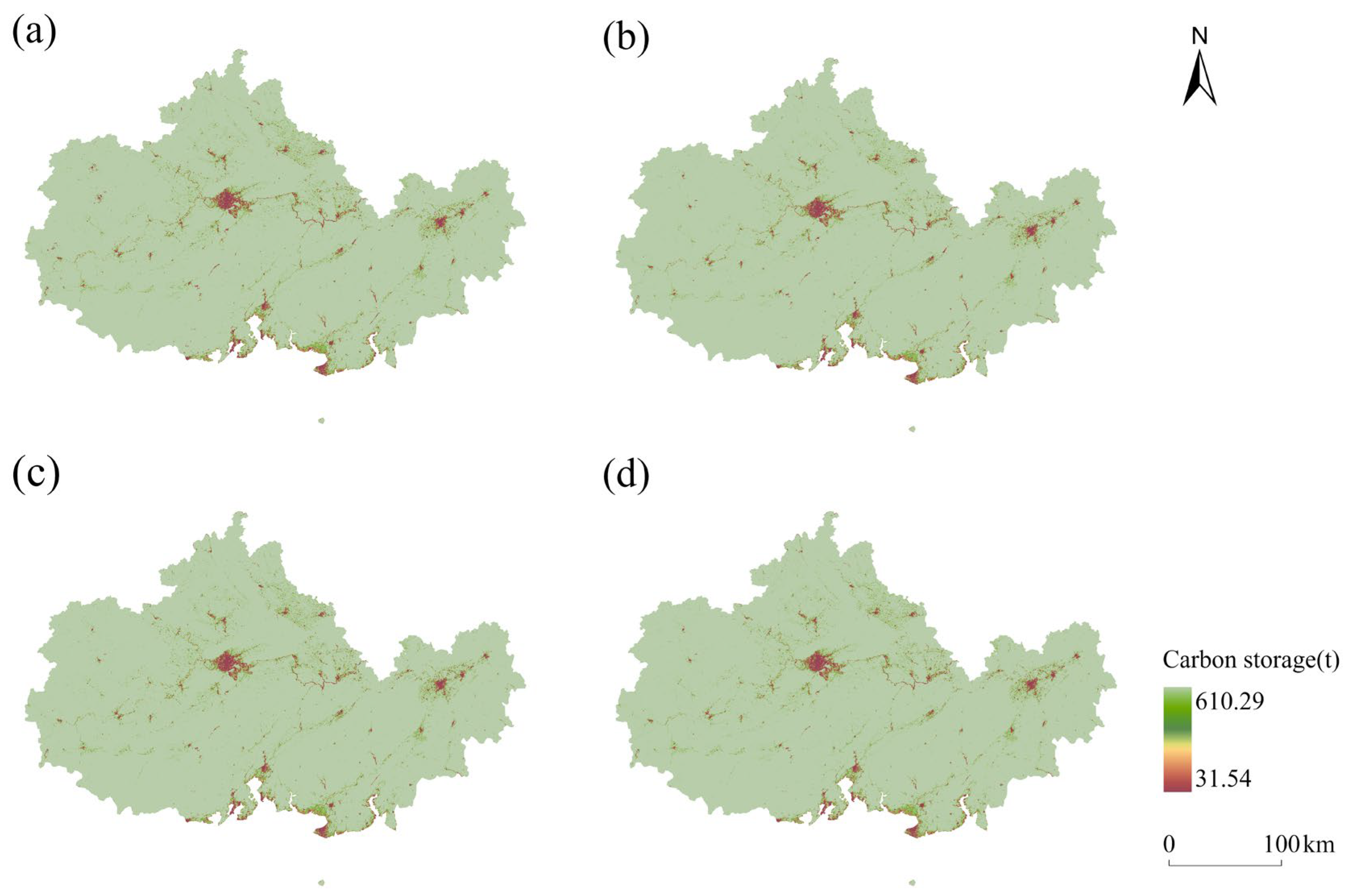
The projected total regional carbon stocks by 2030, ranked from highest to lowest, are as follows: the steep-slope carbon sink enhancement scenario (32,328.83 million tonnes), the low-carbon intensive urbanization scenario (31,574.69 million tonnes), the ecological buffer zone carbon sequestration scenario (31,570.04 million tonnes), and the natural development scenario (31,549.00 million tonnes) (see Table 6 and

Table 8. Carbon storage distribution of various land types under different scenarios during 2030–2035 (million tons).

Scenario	Farmland	Woodland	Grassland	Water	Unused Land	Construction Land	Total
2030 Natural Development Scenario	4328.85	27,097.73	2.24	70.55	0.18	49.46	31,549.00
2030 Steep-slope Carbon Sink Enhancement Scenario	4049.02	28,160.54	2.28	70.95	0.10	45.94	32,328.83
2030 Ecological Buffer Zone Carbon Sequestration Scenario	4343.16	27,107.55	2.30	70.58	0.13	46.32	31,570.04
2030 Low-Carbon Intensive Urban Management Scenario	4347.55	27,109.05	1.84	70.58	0.13	45.55	31,574.69
2035 Natural Development Scenario	4387.64	26,839.51	2.23	70.54	0.18	51.98	31,352.08
2035 Steep-slope Carbon Sink Enhancement Scenario	3917.84	28,763.96	2.27	70.54	0.08	39.08	32,793.77
2035 Ecological Buffer Zone Carbon Sequestration Scenario	4416.47	26,863.33	2.22	70.58	0.13	45.46	31,398.18
2035 Low-Carbon Intensive Urban Management Scenario	4423.87	26,867.39	1.67	70.59	0.12	44.02	31,407.66

Note: In the “ecological buffer zone carbon sink scenario” and the “low-carbon intensive urban management scenario,” farmland area is restricted and remains unchanged; by contrast, the “steep-slope carbon sink enhancement scenario” allows land-use adjustments related to farmland.

and Figure 9). Compared with the baseline natural development scenario, all three anthropogenic regulation scenarios achieved higher total regional carbon stocks. These results confirm that formulating differentiated land-use restriction rules targeting drivers at different levels can increase carbon stocks, constrain the expansion of carbon-stock-loss areas, and effectively mitigate regional mismatches between land-use-change-attributable carbon-stock gains and losses in the short term.

By comparing the simulated outputs for 2030 with the historical dataset for 2025 (Table 6), the following conclusions can be drawn. In 2030, total carbon stock under the natural development scenario is 31,549.00 million tonnes; this value is significantly lower than the 2025 baseline, consistent with the long-term trend of declining carbon stock since 2015. Among the three regulatory scenarios, only the “steep-slope carbon sink enhancement” scenario yields a total carbon stock higher than the 2025 historical level; the other two scenarios merely moderate the rate of decline without reversing the overall trend of carbon loss. The steep-slope carbon-stock-protection scenario yields the most prominent carbon conservation benefits. It increases regional total carbon stock by 779.83 million tonnes compared with the natural development scenario and by 557.21 million tonnes relative to the 2025 baseline. In terms of land-use carbon composition, farmland carbon stock reaches 4049.02 million tonnes, and woodland carbon stock totals 28,160.54 million tonnes, maintaining woodland coverage at the relatively high level observed in 2025. In addition, restoring sloping farmland to woodland and grassland can enhance the carbon-stock retention capacity of farmland. In terms of spatial distribution (Figure 9), the extent of high-value carbon-stock patches expanded markedly within the contiguous karst mountainous area in the northwestern part of the study area. Strict restrictions were imposed on disorderly outward construction land expansion around central cities such as Nanning and Yulin, while the loss of high carbon density woodland in steep-slope areas was largely curbed. The strict construction land prohibition formulated on the basis of the main driving factors (slope and elevation) effectively exerted carbon sink benefits. The low-carbon intensive urban management scenario achieved the second-best optimization outcome among the three regulation-oriented scenarios. Compared with the natural development scenario, it produced modest carbon-stock benefits, yet regional carbon storage still could not approach the 2025 baseline level. This improvement is mainly driven by the effective containment of construction-land sprawl, which reduces carbon loss caused by built-up land conversion. Nevertheless, this scheme only restricts the outward expansion of construction land and does not establish dedicated mountain conservation regulations for woodland and farmland; therefore, it can only moderately reduce carbon-stock losses originating from construction land, but cannot achieve large-scale carbon-stock restoration across the whole region. The ecological buffer-zone carbon-sink scenario ranks third in carbon-sink performance. Benefiting from strictly defined transition constraints that prohibit water-body conversion into other land-use types, woodland and water-body carbon pools within buffer zones around water systems and protected areas remain stable. Continuous sectorized high-value carbon-sink corridors are formed along rivers and nature reserves. However, this regulatory measure mainly acts on linear ecological spaces, resulting in limited regional carbon-stock gains that cannot fully offset carbon losses induced by urban expansion. By 2030, total carbon stock under the natural development scenario is projected to rank lowest among all four scenarios. Combined with spatial distribution maps, construction land continues to expand toward urban centers and the periphery of coastal industrial belts, while scattered woodland patches in the karst mountainous areas of the northwest are gradually being encroached upon. Carbon stock has exhibited a sustained declining trend since 2015, and the spatial mismatch between carbon-stock gains and losses has become increasingly pronounced.

Overall, these three regulation-oriented scenarios had a positive effect on enhancing carbon sink capacity by 2030. However, differences in the stringency of management coverage and land use transition constraints among the scenarios resulted in a clear gradient in carbon sink performance. Under the “Steep-Slope Carbon Sink Enhancement Scenario,” regional carbon stock increased to a level above the 2025 baseline; by contrast, the other two scenarios merely slowed the magnitude of carbon stock decline but could not reverse its downward trend.

3.4.2. Simulation Results for the Year 2035

By 2035, long-term differentiated land management measures will lead to further divergence in regional carbon stock patterns. The four scenarios exhibit increasingly disparate total carbon stock values and distinctly different spatial distributions of carbon pools (Table 6 and Table 8, and Figure 10).

By 2035, total regional carbon stock under the four scenarios is ranked in descending order as follows: the steep-slope carbon-stock-protection scenario (32,793.77 million tonnes), the low-carbon intensive urbanization scenario (31,407.66 million tonnes), the ecological buffer zone carbon-stock-protection scenario (31,398.18 million tonnes), and the natural development scenario (31,352.08 million tonnes). Compared with the 2025 baseline carbon stock of 31,771.62 million tonnes, only the steep-slope carbon-stock-protection scenario achieves a positive carbon stock surplus of 1022.15 million tonnes. The remaining three scenarios exhibit lower carbon stock values than the 2025 baseline, indicating continuous cumulative carbon stock losses due to the absence of long-term mountain ecological conservation constraints. Without sustained ecological restriction mechanisms, urban expansion under the natural development scenario continuously encroaches on valley and piedmont ecological land. By 2035, the total regional carbon stock decreased to 31,352.08 million tonnes, the lowest value among all scenarios over the entire study period and a decline of 419.54 million tonnes relative to the 2025 level. Woodland carbon stock declines to 26,839.51 million tonnes, while construction land carbon stock rises to 51.98 million tonnes. The continued loss of high-carbon-density ecological land further underscores the unsustainability of the current land-use pattern. The ecological advantages of the steep-slope carbon-stock-protection scenario are further amplified. Compared with the natural development scenario, the total regional carbon stock under this scenario increased cumulatively by 1441.69 million tonnes by 2035. From the perspective of land structure, carbon storage of woodland stays steady at 28,763.96 million tons, while farmland carbon storage attains 3917.84 million tons. The carbon stock retention capacity of farmland is improved by restoring sloping farmland to woodland and grassland. As shown in Figure 10, in the karst mountainous area in the northwestern part of the study region, the contiguous high-value carbon-stock zones remain largely intact. The sprawling expansion of coastal cities and towns such as Nanning, Beihai, Qinzhou, and Fangchenggang has been constrained, fundamentally curbing rocky desertification on steep slopes and the loss of carbon stocks. This scenario achieves the simultaneous attainment of multiple objectives—namely, karst ecological restoration, intensive management of construction land, and the stable growth of regional carbon stocks—and yields the optimal carbon-related comprehensive benefits among the three simulated scenarios. The carbon stock values obtained from the ecological buffer zone carbon sequestration scenario and the low-carbon intensive urban management scenario are both higher than the natural development baseline; however, the inherent limitations facing sustained carbon stock restoration have gradually become apparent. By 2035, relative to the 2025 baseline, the regional total carbon stocks under these two scenarios would decrease by 373.44 million tonnes and 363.96 million tonnes, respectively. The ecological buffer zone carbon sequestration scenario relies solely on linear spaces along water systems and protected areas for carbon stock conservation, resulting in limited increases in woodland carbon stocks; whereas the low-carbon intensive urban management scenario only constrains outward urban expansion without establishing conservation regulations for mountainous areas or sloping farmland. Consequently, the carbon stock growth potential of both scenarios is far lower than that of the steep-slope carbon sink enhancement scenario.

A comprehensive analysis of time-series carbon-stock datasets from 2000 to 2025 (Table 6), multi-scenario simulation outputs for 2030 and 2035 (Table 8), and spatial distribution maps of carbon-stock patterns for these two periods (Figure 9 and Figure 10) yields the following findings. The steep-slope carbon-stock-protection scenario matches the composite karst-coastal geomorphic features of the study area and aligns with the three-tier driving-factor system consisting of primary topographic determinants, secondary ecological constraints, and anthropogenic-socioeconomic disturbances. This scenario establishes a sustainable land-use framework that can stabilize regional woodland carbon pools in the long run and keep carbon-stock magnitudes higher than the 2025 baseline. It further facilitates low-carbon-oriented territorial spatial governance. Accordingly, among all simulated scenarios, it represents the best-performing land-use regulation option for carbon-stock conservation.

4. Discussion

4.1. Temporal Differentiation of Carbon Storage in Karst-Coastal Transition Zones of Southern China

Regional carbon stock from 2000 to 2025 presents a fluctuating evolutionary pattern: an initial decrease during 2000–2005, followed by continuous accumulation during 2005–2015, and a gradual decline after 2015. Woodland conversion to construction land serves as the primary driver of regional carbon stock loss. This temporal trend is consistent with the findings of Qiu et al. [43], who conducted research across the entire karst zone of southern China. Qiu et al. confirmed that the Grain for Green Program produces short-term carbon stock accumulation benefits, whereas continuous urban sprawl gradually offsets these ecological restoration gains. Long-term land-system carbon stock evolution in the ecological functional zones of the Yellow River Basin also exhibits a consistent pattern: early-stage carbon stock accumulation followed by later-stage carbon stock loss driven by urban expansion. Chen et al. [44] investigated the long-term evolution of land-use carbon budget in the ecological functional zones of the Yellow River Basin and found that it also exhibited a two-stage characteristic: carbon sink accumulation in the early stage and carbon loss dominated by urban expansion in the later stage. Xie et al. [45] applied long-term LUCC dynamic simulation and verified that ecological protection and the Grain for Green Program promote vegetation expansion. Such vegetation growth increases community biomass and consistently improves ecosystem carbon stock retention capacity, serving as the core positive driver of regional carbon stock growth during 2005–2015. Zhou et al. [22] further indicated that karst regions are characterized by thin soil layers, and soil carbon stock loss caused by land-use transformation is largely irreversible.

The study area exhibits distinct spatial zonation: high-value carbon-stock patches are predominantly distributed in the northwestern karst mountainous zones, while intensive carbon-stock loss clusters occur in the southern coastal urban areas. This finding fills a prevalent research gap in existing studies, which largely focus solely on inland karst regions. Most international evaluations of karst carbon stock changes concentrate on pure plateau karst mountain landscapes and neglect the dual ecological disturbances derived from port industrial development and coastal urban expansion in composite geomorphic zones integrating karst peak clusters and coastal alluvial plains [46,47]. Existing inland karst studies present evident regional limitations. Du et al. investigated plateau karst areas in Guizhou and only characterized rocky desertification restoration and woodland carbon stock evolution, excluding coastal plain zones and ignoring carbon stock disparities caused by coastal industrial land transitions. Shi et al. focused on contiguous inland karst mountains in Southwest China and merely analyzed temporal variations in mountain above-ground vegetation carbon stock, without accounting for intensive human disturbances in coastal zones. Similarly, Ding et al. simulated inland karst watersheds dominated by mountain and valley landforms and formulated conservation strategies only for sloping farmland and mountain woodland, lacking insights into the unique carbon-stock evolution patterns of mountain–coastal ecotones. Yang et al. [48] pointed out that ecotone zones between mountains and coasts constitute vulnerable terrestrial carbon-stock-sensitive ecosystems, where urban sprawl and land reclamation can produce persistent carbon-stock degradation. Their InVEST-based simulation of Yellow River Estuary wetlands further confirmed that coastal construction expansion induces far more severe carbon stock loss than woodland degradation in inland mountainous areas. Different from previous single-landform studies, this research covers three typical geomorphic units: karst peak-cluster terrain, valley farmland, and port construction zones. Based on six phases of long-term 30 m-resolution remote sensing data, this study comprehensively characterizes spatial and temporal disparities in carbon stock across diverse geomorphic environments. Nevertheless, constrained by data accessibility, this study does not quantify the individual contributions of rocky desertification dynamics and karst weathering-related inorganic carbon accumulation to temporal carbon stock variations. Such mechanisms can be further explored through multi-factor coupled models in future research.

4.2. Three-Tier Hierarchical Driving Mechanism of Carbon Budget

Based on the multicollinearity test and results of bivariate LISA spatial autocorrelation, the 12 driving factors were classified into a gradient system including primary terrain-dominated factors, secondary ecological constraint factors, and tertiary socioeconomic disturbance factors, which conforms to the hierarchical logic of karst background, ecological buffer zones, and human development in southern China. Most existing studies on carbon driving forces merely rank factors according to explanatory power without distinguishing spatial management tiers, which provides insufficient support for differentiated scenario formulation. Shi et al. [47] identified driving factors of above-ground carbon storage in Southwest China’s karst regions using random forest and spatial autocorrelation. They only roughly categorized all influencing factors into natural and human-induced groups without establishing an independent ecological buffer tier, failing to fully characterize the cascading effect transmitted sequentially by topographic substrates, ecological barriers, and urban development under karst geomorphology. By adopting bivariate Moran’s I, Bai et al. [49] analyzed agglomeration characteristics of ecosystem services in karst heritage sites. They only ranked factors by explanatory capacity and did not construct a three-tier gradient framework oriented to territorial spatial management and thus could not provide hierarchical evidence for the three differentiated land transition rules targeting steep slopes, water systems, and urban areas. Zong et al. [50] verified that three tiers of driving forces, namely topographic substrates, ecological buffers, and urban development, must be separated for composite coastal mountain-plain regions. Classifying impact factors merely into natural and human categories fails to reflect the regulatory effects generated by intermediate layers. Random forest analysis on soil organic carbon drivers in Southwest China’s karst areas conducted by Li et al. [51] also proves the inherent limitations of the single binary classification framework. Three tiers of factors exert chained interaction effects with sequential transmission, and merging them into two categories will obscure the regulatory function of intermediate layers. From a methodological perspective, conventional global regression and unstratified random forest can only identify average regional correlations while ignoring the spatial hierarchical heterogeneity of driving factors. It is highly likely to cause biased mechanistic interpretation in karst regions characterized by complex terrain and overlapping multiple ecological constraints. In contrast, this study first defines hierarchical tiers of driving forces and further identifies inter-layer spatial interactions combined with bivariate LISA. This framework can accurately capture the differentiated influence intensity of multi-tier factors in karst mountainous areas, valley farmland, and coastal construction zones. Relevant domestic studies focusing on single inland karst regions or pure-plain watersheds deal with relatively homogeneous landforms, without the overlapping constraints of karst rocky desertification and coastal plain geomorphic backgrounds. Therefore, a binary driving-factor framework is sufficient for their analysis. This indirectly demonstrates the pertinence and innovative value of the three-tier gradient driving framework constructed in this study for composite karst-coastal ecotones. It provides solid theoretical support for setting zonal differentiated land transition parameters in the subsequent multi-scenario simulation. It is worth noting that climatic variables, including temperature and precipitation, produce relatively low beta coefficients in this regression model. Climate fundamentally modulates karst vegetation development and carbonate rock weathering over large spatial extents and longtime spans. However, moderate spatial gradients of temperature and precipitation can be observed across the study area, and inter-annual climate fluctuations between 2000 and 2025 remain limited. For this reason, climatic factors serve as stable background conditions, whereas topographic heterogeneity, ecological constraints, and anthropogenic land-use transformations exert dominant controls over the spatiotemporal patterns of the regional carbon budget within the investigated period.

4.3. Limitations of This Study and Common Deficiencies in Carbon Research on Southern China’s Karst Regions

Although the overall findings of this study are robust under the established model configuration, inherent boundary settings of the modelling framework and simulation uncertainties may introduce potential biases in result interpretation. These limitations are ubiquitous and remain common challenges in current studies focusing on karst carbon stock dynamics.

First, the exclusion of karst-weathering-driven inorganic carbon processes, industrial fossil carbon emissions, dynamic rocky desertification parameters, and field-measured carbon density data contributes to combined estimation uncertainties (as stated in Section 2.3.5) [52,53,54]. The omission of karst inorganic carbon accumulation tends to underestimate regional total carbon stock, particularly in karst mountainous areas with intensive carbonate weathering [55]. Since this study adopts carbon density values from existing literature rather than full-coverage field soil sampling, the parameters fail to reflect vertical soil organic carbon heterogeneity under varying rocky desertification degradation gradients, thereby potentially causing localized overestimation or underestimation of soil carbon stock [53]. The application of static rocky desertification status neglects continuous carbon stock loss induced by desertification progression, which may bias the quantified responses of regional carbon stock to ecological restoration and land reclamation measures [54]. In addition, the exclusion of industrial fossil emissions restricts the current assessment to land-use-driven organic carbon stock variations, rather than capturing the complete net carbon balance of the study area [52]. Second, uneven simulation accuracy across different land-use types introduces pixel-scale uncertainties in multi-scenario projections. Grassland and unused land generally occur as fragmented patches and exhibit relatively lower simulation accuracy. Although their limited area proportion cannot reverse the overall regional carbon stock trends, localized estimation biases may exist in these fragmented landscapes. Furthermore, the integrated PLUS-InVEST framework cannot quantify decarbonization benefits derived from industrial restructuring and energy optimization. Accordingly, the low-carbon intensive urban scenario only reflects land-use-based regulatory effects and fails to fully represent the mitigation potential of socioeconomic policies. In addition, this scenario evaluation focuses primarily on carbon stock conservation effects, without systematic multi-objective trade-off analysis concerning grain security, economic input costs, and urban construction demands. Among the three designed scenarios, ecological regulation schemes (steep-slope carbon-stock-protection and ecological buffer conservation scenarios) adopt more elaborate parameter configurations and analytical processing, whereas the low-carbon intensive urban scenario receives relatively simplified treatment. Restricted by the inherent mechanism of the PLUS-InVEST modelling chain, the urban scenario only implements land-use management measures, including built-up sprawl restriction and internal green space optimization, while excluding industrial adjustment and energy-oriented decarbonization pathways. These socioeconomic mitigation approaches remain beyond the modelling scope of this study, representing a notable limitation of the current scenario design. Additionally, constrained by data availability, most socioeconomic and environmental driving factors adopt single-year snapshot data (2020 or 2024) instead of full-period time-series, which may produce subtle bias when representing human-environment patterns over the whole 2000–2025 period.

For future research, targeted field sampling campaigns covering stratified soils along different rocky-desertification and coastal-plain gradients should be conducted to acquire localized carbon-density parameters and mitigate parameter-related estimation biases [53]. Dynamic rocky-desertification evolution modules and karst inorganic-carbon process algorithms can be coupled, together with anthropogenic industrial-energy emission datasets, to construct a complete organic-inorganic integrated carbon-stock accounting framework for karst-coastal ecotones [52,54,55]. Furthermore, incorporating climate-disturbance variables into multi-scenario simulations will help disentangle how temperature and precipitation variations jointly shape vegetation carbon-stock dynamics, karst weathering processes, and rocky-desertification evolution. Comprehensive multi-objective evaluation tools should also be adopted to balance carbon-stock conservation, agricultural production, and socioeconomic requirements for territorial low-carbon governance.

4.4. Policy Implications and Regulation Suggestions

This study investigates the spatiotemporal patterns and hierarchical driving mechanisms of carbon-stock dynamics within the karst-coastal composite ecotone. Combined with multi-scenario simulation outputs, practical territorial regulation strategies are proposed. Characterized by complex geomorphic conditions and fragile ecosystems, the study region suffers from prominent conflicts between urban expansion and ecological conservation. Accordingly, this paper puts forward targeted suggestions for low-carbon-oriented land management. These findings can underpin local low-carbon land governance practices, and offer feasible references for mitigating karst ecological degradation and restraining unregulated coastal urban sprawl.

First, differentiated zonal land-management strategies should be implemented to address spatial heterogeneity in carbon-stock patterns. The northwestern karst mountainous parts of the study area constitute core functional zones for regional carbon-stock preservation. Disturbances such as steep-slope cultivation and unregulated construction-land occupation must be strictly restricted. Ecological restoration measures, including integrated rocky-desertification rehabilitation and Grain-for-Green programs, should be continuously promoted to maintain the fundamental ecological capacity for carbon-stock retention across the region. By comparison, the southern coastal plains and urban corridors experience prominent carbon-stock loss driven primarily by urban land expansion. Uncontrolled outward urban sprawl should be strictly limited, whereas infill development and structural optimization of construction land can effectively reduce ecological carbon-stock losses. Second, a hierarchical regulation framework should be established to support refined carbon-stock governance, consistent with the tiered driving mechanism underlying carbon-stock variations. Topographic variables such as elevation and slope provide the fundamental geographic background. Strict implementation of ecological red-line policies and prohibitions on steep-slope development helps avoid irreversible damage to core carbon pools. Ecological components including vegetation cover, water bodies, and nature reserves serve as critical buffer zones. Rational conservation measures maintain ecosystem stability and improve the resilience of carbon-stock retention. Socio-economic factors, namely population density, economic output, and nighttime light intensity, reflect moderate human disturbances. Reasonable adjustment of industrial layout and land-development intensity supports low-carbon urbanization and alleviates human-driven carbon-stock disturbances. Third, the steep-slope carbon-stock-protection scheme is proposed to balance ecological conservation, carbon-stock preservation, and socio-economic development. Multi-scenario simulation results demonstrate that this solution delivers the most comprehensive performance in terms of carbon-stock retention, rocky-desertification mitigation, and rational land-resource allocation. It can simultaneously constrain karst rocky-desertification, maintain terrestrial carbon-stock levels, and ensure orderly urban development. This high-performance regulation strategy should be incorporated into routine territorial spatial planning. Targeted land-use transition rules need to be formulated for mountain, valley-farmland, and coastal-urban areas, so as to construct a long-term governance mechanism focusing on carbon-stock retention through ecological restoration, carbon-stock loss reduction via built-up-land renewal, and carbon-stock protection through zonal management. This study provides a transferable reference for low-carbon territorial governance and integrated ecological restoration in karst-coastal ecotones globally.

5. Conclusions

By integrating long-term analyses of datasets from 2000–2025, identification of driving factors, and multi-scenario simulation results for 2030–2035, the main conclusions are summarized as follows:

(1)

From 2000 to 2025, land-use patterns and regional carbon-stock dynamics in the karst-coast transitional zone exhibited obvious phased-evolution features. Uncontrolled expansion of construction land triggered the continuous loss of woodland, which dominated regional land-use transformation. The conversion of woodland to construction land constituted the primary driver for regional carbon-stock reduction and spatial carbon-pool degradation.

(2)

The karst–coastal transition zone exhibits significant spatial heterogeneity in carbon stock distribution, forming a clear zonal pattern. The northwestern karst mountainous areas represent core high carbon-stock conservation regions, whereas the southern coastal urban belt experiences severe carbon stock depletion. The spatial differentiation of regional carbon stock is highly consistent with the composite geomorphic features and land-use distribution of the study area.

(3)

Based on linear regression derived standardized Beta coefficients and bivariate local LISA results, this study establishes a three-level hierarchical classification for the 12 influencing factors of land-use-change-attributable carbon-stock-variation. Topographic factors provide fundamental geographic control, and ecological factors exert critical buffering and restrictive effects, whereas socioeconomic and climatic factors produce relatively weak disturbance impacts. Urban expansion constitutes the dominant anthropogenic driver behind regional carbon-stock degradation.

(4)

Multi-scenario simulations verify that differentiated zonal management effectively mitigates carbon stock loss across the karst–coastal transitional ecoregion. Among the three simulation scenarios, the steep-slope carbon-stock-protection scenario achieves the best performance in carbon stock conservation, yielding a cumulative regional carbon stock increment of 1441.69 million tonnes by 2035 while promoting coordinated rocky desertification control and ecological restoration. Notably, this advantage is evaluated solely based on carbon stock indicators under model settings, without considering multi-objective trade-offs such as agricultural production capacity, economic costs, and urban construction demands. Even so, this hierarchical land regulation strategy provides reliable support for sustainable low-carbon development in complex transitional ecological regions.

This study integrates multiple models to elucidate the patterns of carbon stock dynamics and hierarchical governance pathways in the karst–coastal ecotone. Restricted by the absence of datasets regarding inorganic carbon processes, rocky desertification dynamics, and industrial carbon emissions, the current research framework can be further optimized in future studies. The findings provide a reliable quantitative basis for ecological restoration and low-carbon spatial planning in the karst–coastal transition zone of South China.

References

1. United Nations Conference on Environment and Development. United Nations Framework Convention on Climate Change; United Nations: New York City, NY, USA, 1992. [Google Scholar]
2. York, M.; Strange, B.; Khan, A. Drivers of Extreme Carbon Sources and Sinks Across Diverse Ecosystems in the Western USA. Glob. Change Biol. 2026, 32, e70926. [Google Scholar] [CrossRef] [Scilit]
3. Qiu, L.H.; He, J.H.; Yue, C. Substantial terrestrial carbon emissions from global expansion of impervious surface area. Nat. Commun. 2024, 15, 6456. [Google Scholar] [CrossRef] [Scilit]
4. Lyu, M.; Zhou, Y.; Wei, Y.; Li, J.; Wu, S. The Impact of Land Use Changes on Carbon Flux in the World’s 100 Largest Cities. Sustainability 2023, 15, 12497. [Google Scholar] [CrossRef] [Scilit]
5. Lai, L.; Huang, X.J.; Yang, H. Carbon emissions from land-use change and management in China between 1990 and 2010. Sci. Adv. 2016, 2, e1601063. [Google Scholar] [CrossRef] [Scilit]
6. Zhang, R.X.; Yu, H.L.; Chai, Y.Y. Variations of Soil Organic and Inorganic Carbon Stock and Soil Aggregation due to Land Use Change to Urban Green Spaces of Arid Environment. Land Degrad. Dev. 2026, 37, 8372–8386. [Google Scholar] [CrossRef] [Scilit]
7. Jiang, H.X.; Zhen, G.; Cui, T.S. Impacts of land use change on carbon storage in the Guangxi Beibu Gulf Economic Zone based on the PLUS-InVEST model. Sci. Rep. 2025, 15, 6468. [Google Scholar] [CrossRef] [Scilit]
8. Han, R.Y.; Zhang, Q.; Xu, Z.F. Responses of soil organic carbon cycle to land degradation by isotopically tracing in a typical karst area, southwest China. PeerJ 2023, 11, e15249. [Google Scholar] [CrossRef] [Scilit]
9. He, Q.; Li, H.; Xu, C.; Sun, Q.; Bertness, M.D.; Fang, C.; Li, B.; Silliman, B.R. Consumer regulation of the carbon cycle in coastal wetland ecosystems. Philos. Trans. R. Soc. Lond. B Biol. Sci. 2020, 375, 20190451. [Google Scholar] [CrossRef] [Scilit]
10. Cinco-Castro, S.; Herrera-Silveira, J.; Muñoz, J.L.M.; Hernández-Nuñez, H.; Hernández, C.T. Carbon stock in different ecological types of mangroves in a karstic region. Front. For. Glob. Change 2023, 6, 1181542. [Google Scholar] [CrossRef] [Scilit]
11. Shao, M.; Chen, R.; Wang, M.; Zhang, L.; Yan, Y.; Lu, Z. Impact of Land Use Changes on Spatio-Temporal Pattern Evolution of Carbon Storage of Urban Agglomerations in the Yellow River Basin. Ecol. Front. 2026, 46, 1083–1092. [Google Scholar] [CrossRef] [Scilit]
12. Bera, D.; Chatterjee, N.D.; Dinda, S.; Ghosh, S.; Dhiman, V.; Bashir, B.; Calka, B.; Zhran, M. Assessment of Carbon Stock and Sequestration Dynamics in Response to Land Use and Land Cover Changes in a Tropical Landscape. Land 2024, 13, 1689. [Google Scholar] [CrossRef] [Scilit]
13. Masobeng, T.A.; Mapeshoane, B.E.; Marake, M.V.; Ramakhanna, S.J.; Nkunyane, K.F.; Motšoane, M.P.; Moleleki, M.; Teleki, M.; Likoti, M.L.; Lekokotoana, M. Spatio-Temporal Modelling of Soil Organic Carbon Stock Change in Relation to Land Use Changes in Selected Sub-Catchments of Lesotho. Soil Adv. 2025, 4, 100071. [Google Scholar] [CrossRef] [Scilit]
14. Chang, X.; Xing, Y.; Wang, J.; Yang, H.; Gong, W. Effects of land use and cover change on terrestrial carbon stocks in China between 2000 and 2018. Resour. Conserv. Recycl. 2022, 182, 106333. [Google Scholar] [CrossRef] [Scilit]
15. Wei, S.; Xue, Y.; Zhang, M.J. Study on Spatiotemporal Pattern Evolution and Regional Heterogeneity of Carbon Emissions at the County Scale of Major Cities, Inner Mongolia Autonomous Region. Sustainability 2025, 17, 9222. [Google Scholar] [CrossRef] [Scilit]
16. Zhang, H.; Guan, Q.; Zhang, J.; Zhang, T.; Sun, Y.; Zhang, Z. Research on Land Use, Carbon Stocks and Carbon Emissions in Typical Mountainous Areas of the North–South Transition Zone in China: A Case Study of Longnan. Soil Use Manag. 2026, 42, e70190. [Google Scholar] [CrossRef] [Scilit]
17. Chen, J.; Ai, L.; Hao, F.; Su, P.; Feng, X.; Zhao, Y. Spatial Variation of Soil Organic Carbon Stocks in Relation to Land Management Practices: A Case Study From Henan Province, China. Soil Use Manag. 2026, 42, e70185. [Google Scholar] [CrossRef] [Scilit]
18. Yang, H.-X.; He, H.; Liu, B.; Yang, H.-C.; Han, D.-S. Multi-scenario Simulation of Land Use and Carbon Storage Assessment in Arid Region of Northwest China Based on the PLUS-InVEST-Geodetector Model. Huan Jing Ke Xue 2026, 47, 3049–3060. (In Chinese) [Google Scholar] [CrossRef] [Scilit]
19. Pan, C.Y.; Feng, X. Multi-scenario land use simulation for sustainable spatial management using the MOP-PLUS coupled framework: Evidence from the metropolitan fringe of Beijing. J. Environ. Manag. 2026, 410, 130083. [Google Scholar] [CrossRef] [Scilit]
20. Zhang, Y.Y.; Zhang, K.Q.; Wei, S.N. Multi-scenario simulation of spatiotemporal changes of land use and ecosystem services in the plateau mountain city. Sci. Rep. 2026, 16, 23450. [Google Scholar] [CrossRef] [Scilit]
21. Zhou, J.D.; Lu, D.L.; Xu, Y.P. Spatiotemporal evolution of carbon storage in coastal areas of Beibu Gulf, Guangxi based on InVEST and GIS models. Mar. Environ. Sci. 2024, 43, 715–722+732. (In Chinese) [Google Scholar] [CrossRef]
22. Zhou, H.; Tang, M.; Huang, J.; Zhang, J.; Huang, J.; Zhao, H.; Yu, Y. Instability and Uncertainty of Carbon Storage in Karst Regions under Land Use Change: A Case Study in Guiyang, China. Front. Environ. Sci. 2025, 13, 1551050. [Google Scholar] [CrossRef] [Scilit]
23. Wei, C.Q.; Mao, J.X. Spatiotemporal pattern evolution of carbon emissions in Guangxi Beibu Gulf Economic Zone. Sci. Technol. Ind. 2026, 26, 155–163. Available online: http://www.kjhcy.org/kjycy/article/abstract/2026921 (accessed on 10 September 2026). (In Chinese)
24. Sharp, R.; Douaihy, E.; Wolny, S. InVEST, version 3.18.0; User Guide: Carbon Storage and Sequestration Model; Stanford University: Stanford, CA, USA, 2026.
25. Giardina, C.P.; Ryan, M.G. Evidence that decomposition rates of organic carbon in mineral soil do not vary with temperature. Nature 2000, 404, 858–861. [Google Scholar] [CrossRef] [Scilit]
26. Zhang, Z.; Hu, B.Q.; Qiu, H.H. Spatio-temporal Differentiation and Driving Mechanism of Ecological Environment Vulnerability in Southwest Guangxi Karst-Beibu Gulf Coastal Zone. J. Geo-Inf. Sci. 2021, 23, 456–466. (In Chinese) [Google Scholar] [CrossRef]
27. Zhang, Z.; Zhou, Y.; Wang, S.; Huang, X. Comparing Estimation Methods for Soil Organic Carbon Storage in Small Karst Watersheds. Pol. J. Environ. Stud. 2018, 27, 2461–2469. [Google Scholar] [CrossRef] [Scilit]
28. Wang, S.; Zhuang, Q.; Jia, S.; Jin, X.; Wang, Q. Spatial Variations of Soil Organic Carbon Stocks in a Coastal Hilly Area of China. Geoderma 2018, 314, 8–19. [Google Scholar] [CrossRef] [Scilit]
29. Zhang, Z.; Huang, X.; Zhou, Y.; Zhang, J.; Zhang, X. Discrepancies in Karst Soil Organic Carbon in Southwest China for Different Land Use Patterns: A Case Study of Guizhou Province. Int. J. Environ. Res. Public Health 2019, 16, 4199. [Google Scholar] [CrossRef] [Scilit]
30. Patidar, R.; Pingale, S.M.; Khare, D.; Choudhary, S. Assessing Spatio-Temporal Meteorological Drought Dynamics Across Indian Agro-Climatic Zones: A Long-Term Perspective. Int. J. Climatol. 2025, 45, e70146. [Google Scholar] [CrossRef] [Scilit]
31. Liu, Y.; Liu, C.; Wang, S.; Guo, K.; Yang, J.; Zhang, X.; Li, G. Organic Carbon Storage in Four Ecosystem Types in the Karst Region of Southwestern China. PLoS ONE 2013, 8, e56443. [Google Scholar] [CrossRef] [Scilit]
32. Xie, Q.; Han, Y.; Zhang, L.; Han, Z. Dynamic Evolution of Land Use/Land Cover and Its Socioeconomic Driving Forces in Wuhan, China. Int. J. Environ. Res. Public Health 2023, 20, 3316. [Google Scholar] [CrossRef] [Scilit]
33. Hu, C.; Song, M.; Zhang, A. Dynamics of the Eco-environmental Quality in Response to Land Use Changes in Rapidly Urbanizing Areas: A Case Study of Wuhan, China from 2000 to 2018. J. Geogr. Sci. 2023, 33, 245–265. [Google Scholar] [CrossRef] [Scilit]
34. Dormann, C.F.; Elith, J.; Bacher, S.; Buchmann, C.; Carl, G.; Carré, G.; Marquéz, J.R.G.; Gruber, B.; Lafourcade, B.; Leitão, P.J.; et al. Collinearity: A Review of Methods to Deal with It and a Simulation Study Evaluating Their Performance. Ecography 2013, 36, 27–46. [Google Scholar] [CrossRef] [Scilit]
35. Kim, J.H. Multicollinearity and Misleading Statistical Results. Korean J. Anesthesiol. 2019, 72, 558–569. [Google Scholar] [CrossRef] [Scilit]
36. Anselin, L. Local indicators of spatial association—LISA. Geogr. Anal. 1995, 27, 93–115. [Google Scholar] [CrossRef] [Scilit]
37. Getis, A.; Aldstadt, J. Constructing the Spatial Weights Matrix Using a Local Statistic. Geogr. Anal. 2004, 36, 90–104. [Google Scholar] [CrossRef]
38. Yang, Y.; Wang, H.; Gao, Y.; Ge, C.; Wu, J. Spatio-Temporal Relationship and Transition Patterns of Ecosystem Service Value and Land-Use Carbon Emissions on the Loess Plateau. Land 2025, 14, 1764. [Google Scholar] [CrossRef] [Scilit]
39. Liang, X.; Guan, Q.F.; Clarke, K.C.; Liu, S.; Wang, B.; Yao, Y. Understanding the drivers of sustainable land expansion using a patch-generating land use simulation (PLUS) model: A case study in Wuhan, China. Comput. Environ. Urban Syst. 2021, 85, 101569. [Google Scholar] [CrossRef] [Scilit]
40. Yang, Y.-C.; Huang, X.-H.; Wei, J.-Y.; Liao, L.-P.; Feng, G.-Q.; Sun, D.-Y.; Fu, Z.-Y.; Mo, C.-X.; Li, X.-G.; Sun, G.-K. Urban expansion drivers and land use scenario simulation in Nanning, China, using the PLUS model. Sci. Prog. 2026, 109, 00368504261417161. [Google Scholar] [CrossRef] [Scilit]
41. Gong, J.; Du, H.; Sun, Y.; Zhan, Y. Simulation and Prediction of Land Use in Urban Agglomerations Based on the PLUS Model: A Case Study of the Pearl River Delta, China. Front. Environ. Sci. 2023, 11, 1306187. [Google Scholar] [CrossRef] [Scilit]
42. Ding, C.; Zhou, Z.; Wang, C.; Kong, J.; Wang, Y.; Xie, R. Multi-scenario simulation of LULC and carbon dynamics in karst regions using the PLUS model. Front. Environ. Sci. 2025, 13, 1640766. [Google Scholar] [CrossRef] [Scilit]
43. Qiu, S.; Peng, J.; Quine, T.A.; Green, S.M.; Liu, H.; Liu, Y.; Hartley, I.P.; Meersmans, J. Unraveling Trade-Offs Among Reforestation, Urbanization, and Food Security in the South China Karst Region: How Can a Hinterland Province Achieve SDGs? Earth’s Future 2022, 10, e2022EF002867. [Google Scholar] [CrossRef] [Scilit]
44. Chen, X.; Wei, W.; Wei, X.; Xie, B.; Pei, Y.; Zhou, J.; Sherif, M.; Wang, X.; Dewan, A. Spatio-Temporal Changes of Land Use Carbon Emission/Absorption and Its Future Trend in Important Ecological Functional Areas—A Case Study in the Yellow River Basin. Land Degrad. Dev. 2025, 37, 1792–1809. [Google Scholar] [CrossRef] [Scilit]
45. Xie, L.; Wang, H.; Liu, S. The Ecosystem Service Values Simulation and Driving Force Analysis Based on Land Use/Land Cover: A Case Study in Inland Rivers in Arid Areas of the Aksu River Basin, China. Ecol. Indic. 2022, 138, 108828. [Google Scholar] [CrossRef] [Scilit]
46. Du, S.; Zhou, Z.; Huang, D.; Zhang, F.; Deng, F.; Yang, Y. The Response of Carbon Stocks to Land Use/Cover Change and a Vulnerability Multi-Scenario Analysis of the Karst Region in Southern China Based on PLUS-InVEST. Forests 2023, 14, 2307. [Google Scholar] [CrossRef] [Scilit]
47. Shi, J.; Yu, L.; Fang, H.; Zhang, K.; Wigneron, J.-P.; Li, X.; Cui, T.; Liu, C.; Jiao, Y.; Wang, D. Dynamics of Aboveground Carbon Across Karst Terrestrial Ecosystems in China from 2015 to 2021. Forests 2024, 15, 2143. [Google Scholar] [CrossRef] [Scilit]
48. Yang, X.; Wang, C.; Liu, C.; Liu, Z.; Liu, B.; Xu, C. Assessing the spatio evolution of carbon sequestration and optimizing ecological restoration strategies using the InVEST model: A case study of the Yellow River Estuary, China. Mar. Environ. Res. 2025, 209, 107204. [Google Scholar] [CrossRef] [Scilit]
49. Bai, X.; Xiong, K.; Chen, Y.; Liu, Z. Spatiotemporal Evolution of Landscape Stability in World Heritage Karst Sites: A Case Study of Shibing Karst and Libo-Huanjiang Karst. Herit. Sci. 2024, 12, 215. [Google Scholar] [CrossRef] [Scilit]
50. Zong, S.; Hu, Y.; Bai, Y. Spatio-Temporal Pattern and Driving Mechanisms of Land Use Conflicts Changes (2010–2018) in the Bohai Rim Transition Zone. Land Degrad. Dev. 2023, 34, 3451–3466. [Google Scholar] [CrossRef] [Scilit]
51. Li, Q.; Chen, B.; Yuan, H.; Li, H.; Zhuang, S. Characterization of Controlling Factors for Soil Organic Carbon Stocks in One Karst Region of Southwest China. PLoS ONE 2024, 19, e0296711. [Google Scholar] [CrossRef]
52. Qin, Y.; Li, H. Spatial Kernel Density Assessment and Driving Factors Detection of Carbon and Pollution Reduction Synergies in Yangtze and Yellow River Regions: A Marginal Abatement Cost Perspective. Asia-Pac. J. Reg. Sci. 2026, 10, 20. [Google Scholar] [CrossRef] [Scilit]
53. Sheng, M.; Xiong, K.; Wang, L.; Li, X.; Li, R.; Tian, X. Response of Soil Physical and Chemical Properties to Rocky Desertification Succession in South China Karst. Carbonates Evaporites 2018, 33, 15–28. [Google Scholar] [CrossRef] [Scilit]
54. Xie, L.; Deng, Y.; Wang, B.; Qin, H.; Fang, J.; Cao, F.; Wu, L. Changes in soil microbial biomasses and their quotients over the succession of karst rocky desertification. In Proceedings of the 3rd International Conference on Advances in Energy and Environmental Science; Atlantis Press: Dordrecht, The Netherlands, 2015. [Google Scholar] [CrossRef] [Scilit]
55. Nie, T.; Zhou, K.; Zhang, F.; Zhai, X.; Li, W.; Wang, H.; Sun, C.; Kang, Z.; Hu, X.; Ning, W.; et al. Spatial Heterogeneity and Controls of Sedimentary Organic Carbon Distribution in Different Types of Coastal Wetland. Catena 2026, 273, 110409. [Google Scholar] [CrossRef] [Scilit]
Figure 1. Overview of the study area. (a) Location map of southern China. The red shaded area denotes the study area of the Beibu Gulf karst-coastal transition zone; (b) Spatial distribution of Digital Elevation Model (DEM) across the study area; (c) Spatial pattern of baseline land use types in 2025.
Land 15 01747 g001
Figure 2. Land use maps for 2000–2025: (a) 2000, (b) 2005, (c) 2010, (d) 2015, (e) 2020, (f) 2025.
Land 15 01747 g002
Figure 3. Chord diagram of land use transitions during 2000–2025. (a) 2000–2005, (b) 2005–2010, (c) 2010–2015, (d) 2015–2020, (e) 2020–2025. The width of lines represents the area magnitude of land conversion.
Land 15 01747 g003
Figure 4. Spatial distribution of carbon storage from 2000 to 2025. (a) 2000, (b) 2005, (c) 2010, (d) 2015, (e) 2020, (f) 2025. Carbon-storage values represent total carbon mass (tonnes) per 30 m pixel. Blue tones correspond to areas with high carbon storage dominated by woodland, while warm-color areas indicate regions of low carbon storage.
Land 15 01747 g004
Figure 5. Spatial patterns of land-use-change-attributable carbon-stock variation for five discrete periods. (a) 2000–2005, (b) 2005–2010, (c) 2010–2015, (d) 2015–2020, (e) 2020–2025. Variation values represent total carbon mass (tonnes) per 30 m pixel. This dataset quantifies changes in terrestrial carbon stock induced exclusively by land-cover conversions, based on static land-use carbon density parameters from the InVEST model; it does not represent real-time atmospheric CO2 fluxes. The map visualizes four categories for non-zero carbon-stock variation: high-intensity carbon-stock-loss areas, low-intensity carbon-stock-loss areas, low-intensity carbon-stock-gain areas, and high-intensity carbon-stock-gain areas. Pixels with exact zero carbon-stock change indicate no stock alteration triggered by land-use transition and are not symbolized within the four displayed map classes.
Land 15 01747 g005
Figure 6. Sankey diagram of carbon-stock-change flows among different land-use types, 2000–2025. This diagram characterizes carbon-stock-change flows across land-use categories driven by land-use conversions during the study period, reflecting carbon-stock loss and carbon-stock gain induced by land transitions. The width of each flow denotes the magnitude of carbon-stock-change flows between land-use categories.
Land 15 01747 g006
Figure 7. Spatial distribution of bivariate LISA clusters between the 12 driving factors and land-use-change-attributable carbon-stock-variation. (a) Distance to road; (b) DEM elevation; (c) FVC (Fractional Vegetation Cover); (d) GDP density; (e) Precipitation; (f) Slope; (g) Population density; (h) Distance to water system; (i) Soil type; (j) Temperature; (k) Nighttime light intensity; (l) Distance to nature reserves. Red represents high-high (HH) clusters, blue denotes low-low (LL) clusters, pink represents high-low (HL) spatial outliers, and light-blue represents low-high (LH) spatial outliers. Grey areas indicate regions without statistically significant spatial association.
Land 15 01747 g007aLand 15 01747 g007b
Figure 8. Spatial distribution of significance p-values for driving factors. (a) Distance to road; (b) DEM elevation; (c) FVC (Fractional Vegetation Cover); (d) GDP density; (e) Precipitation; (f) Slope; (g) Population density; (h) Distance to water system; (i) Soil type; (j) Temperature; (k) Nighttime light intensity; (l) Distance to nature reserves. Green areas represent regions with p < 0.05, indicating significant spatial correlation between driving factors and carbon budget within these grid units.
Land 15 01747 g008aLand 15 01747 g008b
Figure 9. Spatial distribution of carbon storage under different scenarios in 2030. (a) Natural development scenario; (b) Steep-slope carbon sink enhancement scenario; (c) Ecological buffer zone carbon sequestration scenario; (d) Low-carbon intensive urban management scenario.
Land 15 01747 g009
Figure 10. Spatial distribution of carbon storage under different scenarios in 2035. (a) Natural development scenario; (b) Steep-slope carbon sink enhancement scenario; (c) Ecological buffer zone carbon sequestration scenario; (d) Low-carbon intensive urban management scenario.
Land 15 01747 g010