Article

Urban Vitality in Metropolitan Fringe Areas as Land-Use Transition Interfaces: Nonlinear Associations with the Built Environment in the Chengdu Metropolitan Area, China


1
Department of Urban and Rural Planning, School of Architecture, Southwest Jiaotong University, Chengdu 611756, China
2
Urban Transportation Research Unit, Department of Urban Engineering, The University of Tokyo, Tokyo 113-8656, Japan
*
Author to whom correspondence should be addressed.
Land 2026, 15(8), 1380; https://doi.org/10.3390/land15081380
Submission received: 21 June 2026 / Revised: 26 July 2026 / Accepted: 29 July 2026 / Published: 31 July 2026

Abstract

Metropolitan fringe areas are transitional spaces where urban expansion, industrial relocation, residential spillover, transport infrastructure, and ecological recreation jointly reshape land-use functions. However, urban vitality research has mainly focused on central urban areas, leaving limited evidence on how activity intensity is organized in metropolitan fringe spaces. Taking the Chengdu Metropolitan Area, China, as a case, this study delineates metropolitan fringe areas using POI kernel density analysis and density–distance relationships, calibrated with impervious-surface and remote-sensing evidence, measures village-level relative activity intensity using Baidu heatmap data, and examines nonlinear associations between built-environment variables and urban vitality using LightGBM and SHAP. The results show that vitality across the delineated fringe does not form a uniform core–periphery gradient. Instead, high-vitality units are clustered around industrial parks, residential spillover zones, transport corridors, public-service nodes, and ecological recreation spaces. Population density, nighttime light, gross domestic product, building density, and commercial POI density are the main predictors in both weekday and weekend models. Several variables show nonlinear and saturation-like associations rather than simple linear effects. These findings suggest that higher predicted fringe vitality is more likely to occur where population concentration, development intensity, service provision, transport linkage, and socioeconomic activity coexist, rather than where densification occurs alone. The study extends urban vitality research to metropolitan fringe areas and provides evidence for differentiated land-use planning in urban-rural transition zones.

1. Introduction

1.1. Metropolitan Fringe Areas as Land-Use Transition Interfaces

As urbanization increasingly shifts from the expansion of individual cities to the coordinated development of metropolitan areas and urban agglomerations, the spatial links among urban cores, peripheral towns, and rural settlements have become more intensive [1]. Metropolitan areas have therefore become important regional units for understanding population mobility, industrial coordination, commuting, public-service sharing, and land-use transition [2,3]. Within this spatial structure, metropolitan fringe areas are not merely outer zones beyond the built-up area. They are transitional interfaces where urban expansion, industrial relocation, residential spillover, transport infrastructure, ecological spaces, and rural functions interact and reshape land-use patterns [2,4,5].
Existing studies have described such spaces using related concepts, including the urban fringe, peri-urban areas, urban-rural interfaces, and rural-urban transition zones. Although these concepts differ in origin and emphasis, they commonly point to spaces characterized by mixed land functions, fragmented spatial forms, uneven infrastructure provision, and complex governance boundaries [4,5]. Recent applications of points of interest, nighttime light, remote sensing imagery, road networks, and mobile-positioning data have shifted fringe-area identification from administrative or experience-based delineation toward quantitative approaches based on functional density, construction intensity, and spatial connectivity [6,7]. However, most existing studies still emphasize morphological identification and land-use change, while paying less attention to whether and how these transitional spaces actually support human activity.
From the perspective of land-use performance, the effective use of metropolitan fringe areas cannot be evaluated only by the amount of construction land or development intensity. It also depends on whether these spaces can continuously support production, residence, consumption, commuting, public services, and leisure activities [8]. Urban vitality, which reflects the intensity and spatial concentration of human activities, provides a useful entry point for evaluating the functional operation of fringe areas [9,10]. Introducing urban vitality into metropolitan fringe research therefore helps shift the analytical focus from land-use form to land-use functioning, which is directly relevant to urban-rural integration and metropolitan land governance.

1.2. Urban Vitality Research and the Limits of Central-City Experience

Urban vitality generally refers to the capacity of urban spaces to attract, accommodate, and sustain human activities [11]. Classical urban theories emphasize that mixed functions, short blocks, relatively high density, walkable environments, and continuous street activities are important conditions for vitality [9,10,12]. With the development of urban big data, vitality studies have gradually moved from field observations, questionnaires, and statistical yearbooks to quantitative analyses based on points of interest, mobile-phone data, social media check-ins, transport trajectories, nighttime light, and internet heatmap data [13,14,15]. These data sources have improved the ability to identify the spatial distribution, temporal variation, and functional differentiation of human activities.
Previous studies have mainly focused on central urban areas, commercial centers, street blocks, rail-station areas, or intra-urban neighborhoods, and have commonly found that population concentration, commercial facilities, road connectivity, public transport, public services, and functional diversity are closely associated with urban vitality [16,17,18,19]. In dense central urban areas, these variables often explain activity intensity because such areas are characterized by continuous street interfaces, mixed functions, compact development, and dense public transport networks [17]. However, these central-city findings cannot be directly extended to metropolitan fringe areas.
Vitality in metropolitan fringe areas is shaped by multiple land-use functions. Industrial parks may generate concentrated weekday activities; residential spillover areas may become more active in the evening and on weekends; transport corridors may produce node-based or short-term activity concentrations through commuting and logistics; and ecological recreation spaces may attract visitors mainly on weekend [2,3,20,21]. Such activity structures differ from the continuous street life of central urban areas and from the low-density residential pattern of conventional suburbs [4]. Therefore, fringe vitality may not follow a simple linear decline from the urban core, but may instead appear as nodes, corridors, patches, and temporally differentiated activity clusters. Directly applying central-city vitality mechanisms to metropolitan fringe areas may underestimate their functional complexity and misrepresent their planning needs.

1.3. Built Environment and the Nonlinear Turn in Vitality Studies

The built environment provides an important spatial basis for explaining differences in urban vitality. In transport and land-use research, the 5D framework usually characterizes the built environment in terms of density, design, diversity, destination accessibility, and distance to transit [22,23]. In urban vitality research, population density, building density, commercial facilities, public services, road networks, public transport stations, functional mix, and green space have been widely used to explain differences in human activity intensity [17,24]. In recent years, nighttime light, gridded gross domestic product, normalized difference vegetation index, building footprints, and high-resolution remote sensing data have also been incorporated into vitality research, expanding built-environment analysis from traditional land-use variables to multidimensional indicators of socioeconomic conditions, ecological background, and construction intensity [17,25].
However, the relationship between the built environment and urban vitality is not always linear. Increasing attention has been paid to value ranges, marginal effects, saturation patterns, and interactions among built-environment variables [26,27,28]. Traditional linear regression, spatial regression, and geographically weighted regression can reveal overall correlations or spatial heterogeneity, but they are less flexible in capturing nonlinear relationships and high-order interactions unless these terms are explicitly specified [27]. Machine-learning methods such as random forest, gradient boosting, and XGBoost provide useful tools for modeling complex associations and have been increasingly applied in urban vitality, travel behavior, land-use, and built-environment studies [27,29,30]. At the same time, interpretable machine-learning methods such as SHapley Additive exPlanations help explain the direction, strength, and potential nonlinear contribution of variables to model predictions, thereby reducing the “black-box” problem of machine-learning models [31].
This nonlinear perspective is particularly relevant to metropolitan fringe areas. Because fringe areas contain different development stages, mixed land functions, and unstable land-use structures, some built-environment variables may be associated with vitality only within certain value ranges [27]. For example, building density in central urban areas often represents intensive development, whereas in fringe areas it may first indicate whether basic spatial conditions for activity have been formed. Similarly, high normalized difference vegetation index values may indicate low construction intensity in central areas, but may also represent greenways, parks, suburban recreation spaces, and ecological consumption destinations in fringe areas [17,24,32]. Functional mix may support vitality in compact central areas, but excessive or poorly coordinated mix in fringe areas may reflect functional fragmentation rather than effective urbanity. Therefore, the meanings of built-environment variables need to be interpreted in relation to land-use transition contexts.

1.4. Research Gap and Our Study

Existing research provides important evidence on urban vitality and its built-environment correlates, but three gaps remain. First, most vitality studies focus on central urban areas or intra-urban neighborhoods, while the vitality patterns of metropolitan fringe areas remain insufficiently examined [16,24]. Second, fringe-area delineation still often depends on administrative boundaries, built-up area boundaries, or experience-based judgment, which may fail to capture transitional spaces formed by functional facility agglomeration and metropolitan spatial linkages [3,6]. Third, although nonlinear built-environment associations have received increasing attention, existing evidence mainly comes from central urban areas or high-density blocks, and the contextual meanings of nonlinear associations in metropolitan fringe areas remain unclear [27,28].
To address these gaps, this study takes the Chengdu Metropolitan Area as an empirical case. It first delineates metropolitan fringe areas using POI kernel density and density–distance curves, and then measures village-level weekday and weekend urban vitality using Baidu heatmap data. It further applies LightGBM and SHapley Additive exPlanations to examine nonlinear associations between built-environment variables and vitality. The study asks three questions: (1) How are metropolitan fringe areas spatially delineated from the perspective of functional facility density? (2) How does urban vitality vary across fringe areas on weekdays and weekends? (3) Which built-environment variables are most strongly associated with fringe vitality, and how do their associations vary nonlinearly? By answering these questions, this study extends urban vitality research to land-use transition interfaces and provides empirical evidence for differentiated planning in metropolitan fringe areas.
This study contributes to the existing literature in three respects. First, it reconceptualizes metropolitan-fringe vitality as a heterogeneous and discontinuous spatial phenomenon organized through functionally differentiated nodes, corridors, and patches, rather than as a uniformly declining extension of central-city vitality. Second, it extends the interpretation of land-use transition from changes in land-cover composition to the functional reorganization of production, residence, transport, services, and ecological recreation, thereby linking land-use transition more directly to the spatial performance of human activities. Third, it advances built-environment vitality research by showing that the predictive relevance of density, accessibility, services, and socioeconomic activity is nonlinear and context dependent in fringe areas, highlighting development stages, diminishing returns, and functional coordination rather than the maximization of individual attributes. These contributions provide a basis for differentiated planning across distinct metropolitan-fringe contexts.

2. Method

2.1. Study Area

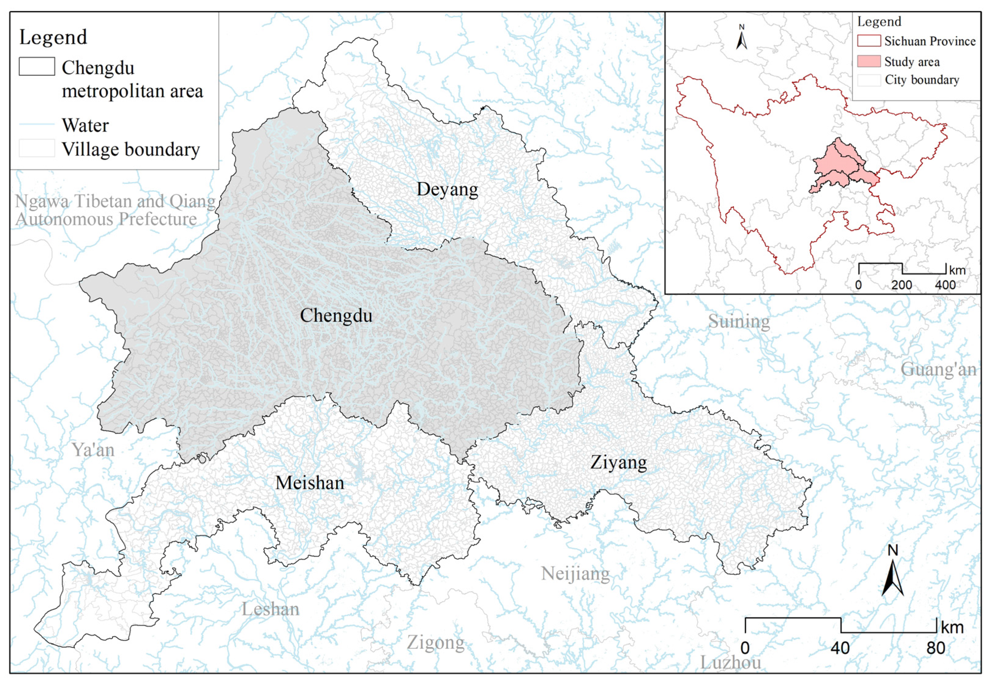
The Chengdu Metropolitan Area is located in the core of the Chengdu Plain Economic Zone in western China and includes Chengdu, Deyang, Meishan, and Ziyang (Figure 1). The area covers approximately 33,100 km2 and is one of the most important metropolitan regions in western China in terms of population concentration, industrial development, and transport connectivity [33]. In recent years, the integration of Chengdu, Deyang, Meishan, and Ziyang has strengthened intercity industrial coordination, transport infrastructure, public-service sharing, and ecological-space governance [34]. In this study, village-level administrative units were used as the basic spatial units for vitality measurement and built-environment analysis because they provide relatively fine-grained governance units for examining intra-fringe differences and are directly relevant to land-use governance and rural–urban integration planning.
The Chengdu Metropolitan Area provides a suitable empirical context for examining fringe vitality because it combines a dominant core city, surrounding medium-sized cities, industrial relocation, new-town development, transport corridor expansion, and ecological recreation resources. These conditions make its fringe areas different from both conventional suburbs and purely rural transition zones. Therefore, the case provides an opportunity to examine whether vitality in metropolitan fringe areas follows a continuous core-periphery gradient or is organized through functionally differentiated nodes, corridors, and patches.
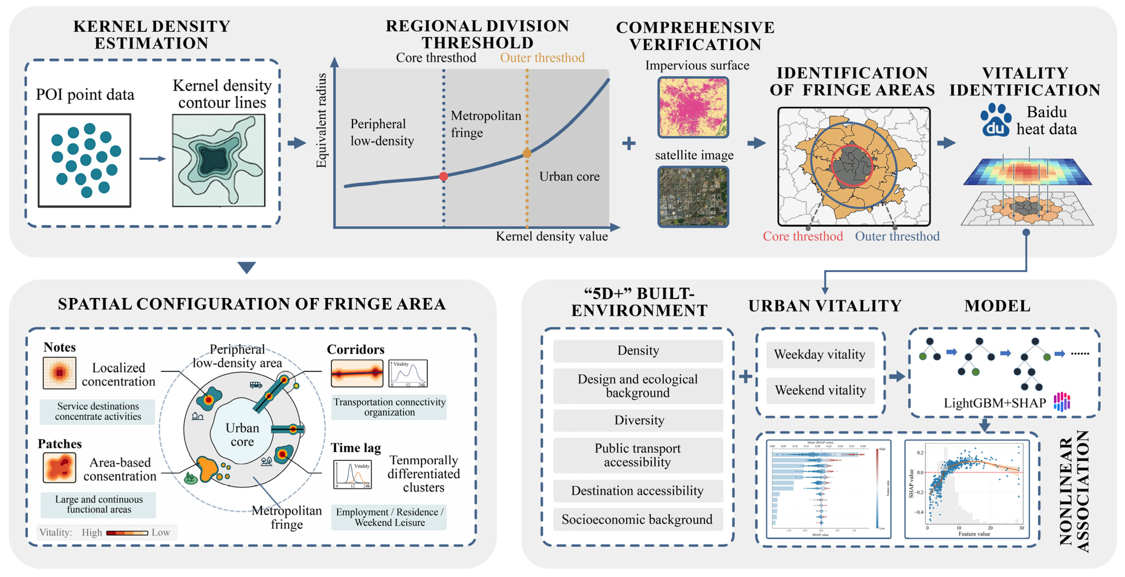
Figure 2 presents the conceptual and analytical framework of this study. Metropolitan fringe areas are understood as land-use transition interfaces formed through the spatial reorganization of production, residence, transport, public services, and ecological functions. This reorganization produces discontinuous spatial configurations, including activity nodes, development corridors, and functional patches, as well as temporally differentiated weekday and weekend rhythms. Within this framework, built-environment attributes are not assumed to affect vitality independently or linearly. Instead, they represent complementary spatial conditions whose predictive associations may vary across development stages and functional contexts. The empirical analysis therefore links fringe-area delineation, vitality measurement, functional interpretation, and nonlinear built-environment modeling.

2.2. Data Sources and Variable Construction

Based on the 5D built-environment framework and the characteristics of metropolitan fringe areas, this study constructed a 5D+ indicator system [22,23]. The indicator system includes six dimensions: density, design and ecological background, diversity, public transport accessibility, destination accessibility, and socioeconomic background (Table 1).
The density dimension includes population density and building density, which represent the population base and development intensity, respectively. The design and ecological background dimension includes road density and normalized difference vegetation index. Road density reflects road-network connectivity and corridor linkage, while normalized difference vegetation index captures vegetation cover, ecological space, and potential recreation environments. The diversity dimension is represented by POI functional mix. Public transport accessibility includes public transport station density and distance to the nearest public transport station. Destination accessibility includes commercial POI density, public-service POI density, employment POI density, and residential POI density. The socioeconomic background dimension includes nighttime light and gross domestic product.
According to urban land-use functions and the purpose of this study, commercial, public-service, employment, and residential POI densities were calculated separately. POI functional mix was calculated independently using the finer-grained categories retained from the original Amap POI classification and the Shannon diversity index [35]:
M i x i = c = 1 C p i c ln p i c , p i c = N i c c = 1 C N i c
where M i x i denotes the POI functional mix of village unit i, C is the number of POI categories, and p i c is the proportion of points of interest of category c in unit i. A higher value indicates that the unit contains more diverse and more evenly distributed POI functions.
All spatial data were projected into the same coordinate system, clipped to the study area, checked for abnormal values, and spatially matched to village-level administrative units. Points of interest, public transport stations, and population data were aggregated by count or total value. Road data were summarized by road length within each unit. Building footprints were aggregated by building footprint area. Raster data, including nighttime light, gross domestic product, and normalized difference vegetation index, were extracted as mean values within each village unit.

2.3. Delineation and Validation of Metropolitan Fringe Areas

The delineation of metropolitan fringe areas is a critical step in this study because it determines the spatial sample for subsequent vitality measurement and built-environment modeling. Traditional delineation methods often rely on administrative boundaries, built-up area boundaries, or population statistics. However, metropolitan fringe areas frequently cross administrative units and contain heterogeneous land-use functions; therefore, administrative boundaries alone cannot adequately represent their transitional nature [3,7,36]. This study delineated metropolitan fringe areas using POI kernel density estimation and density–distance curves, with the aim of identifying transitional spaces between high-density urban cores and low-density peripheral areas from the perspective of functional facility agglomeration.
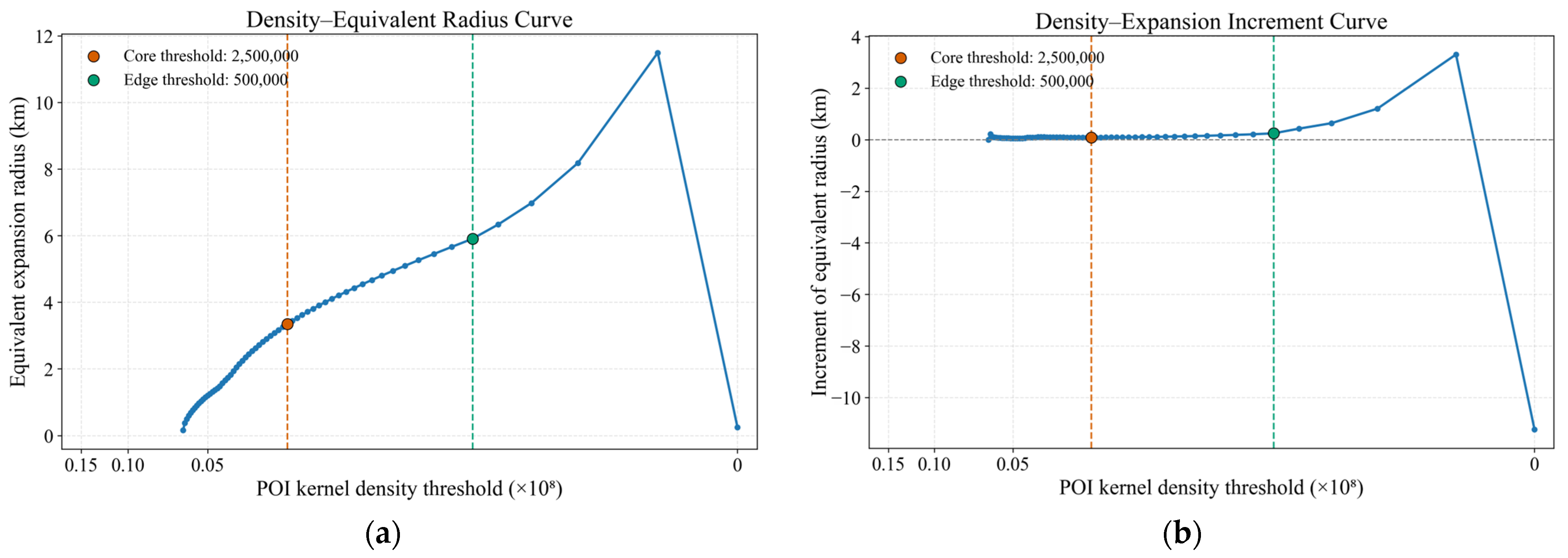
Kernel density estimation was conducted separately for Chengdu, Deyang, Meishan, and Ziyang to avoid the dominance of the Chengdu urban core masking the center–fringe structures of the surrounding cities. The kernel-density search radius was set to 2 km, with an output cell size of 5 m. After duplicate removal and coordinate correction, all POI categories were used to generate continuous density surfaces representing functional facility agglomeration. Density contours were extracted from each surface, and density–equivalent radius curves and density–expansion increment curves were constructed to identify the transition from compact urban cores to metropolitan fringe areas.
For a given POI density threshold dj, the area enclosed by the corresponding density contour was denoted as A d j . The equivalent expansion radius was calculated as:
S j = A d j π
The expansion increment between two adjacent density thresholds was calculated as:
S j = S j S j 1
As the density threshold decreases, the contour generally expands from the urban core to peripheral areas. A slow expansion at high density values indicates the compact urban core, whereas a rapid increase in S j suggests the transition from the core to the fringe. When the density threshold decreases further and the expansion increment becomes stable or changes again, the outer boundary of the fringe area can be identified.
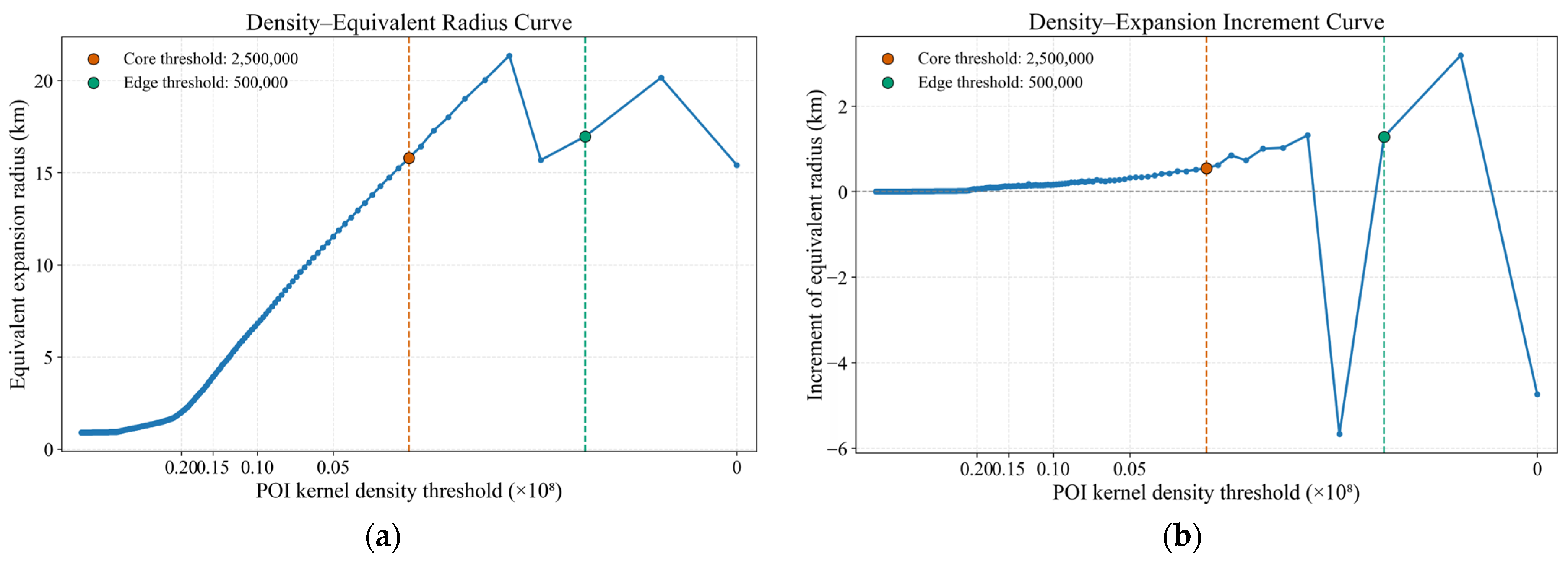
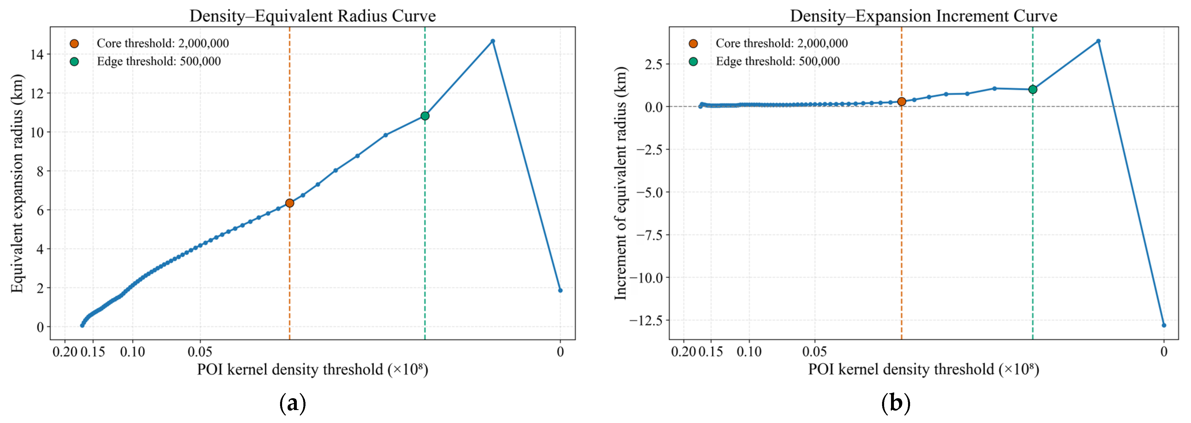
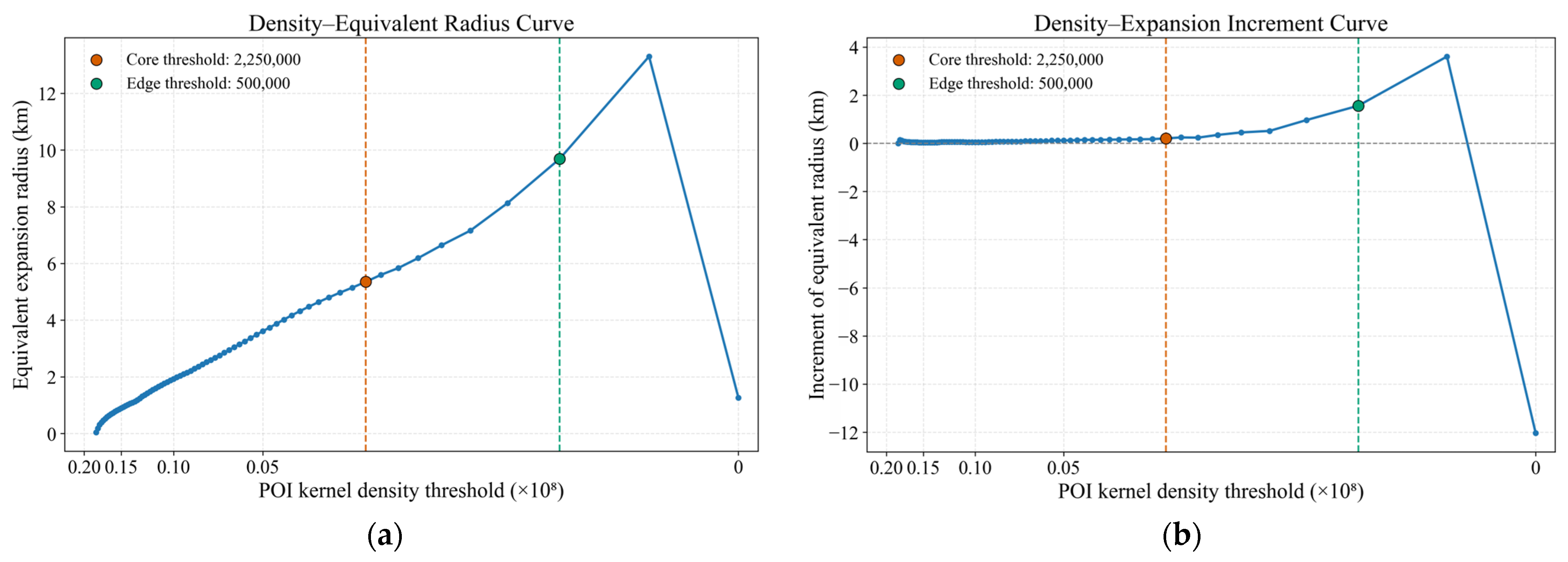
The preliminary core and outer-fringe thresholds were identified by examining changes in the density-equivalent radius curve and the density-expansion increment curve. To reduce the subjectivity of visual interpretation, the candidate thresholds were first determined from local changes in the expansion increment curve and then checked against impervious surface, road-network distribution, and built-up spatial morphology. The final delineation was conducted separately for the four cities, and the identified thresholds are reported in Appendix A Figure A1, Figure A2, Figure A3 and Figure A4. The delineated fringe polygons were overlaid with village-level administrative units. A village unit was included in the analytical sample if more than 50% of its area overlapped with the delineated fringe area. The sensitivity of different overlay thresholds (30%, 40%, 50%, 60%, and 70%) was further examined to assess the robustness of the delineation results. Based on the comparative analysis, the 50% overlap threshold was selected as the optimal criterion, and the sensitivity analysis results are provided in Appendix A Table A1. This rule was adopted to ensure that the selected units were mainly located within the transitional fringe zone and to avoid including units with only marginal spatial intersection. Based on this criterion, 786 village-level units were selected for subsequent analysis.

2.4. Measurement of Urban Vitality and Temporal Difference

Baidu heatmap data were used to represent the relative intensity of human activities in metropolitan fringe areas. The data were collected from 10 July to 16 July 2023 at an hourly interval and were converted into 200 m × 200 m raster grids. The period includes five weekdays and two weekend days, representing short-term relative activity intensity during a specific non-holiday week (Table 2). Because Baidu heatmap values are relative activity-intensity indicators rather than direct population counts, this study interprets them as relative comparative indicators of activity intensity across village units and time periods. Zero-valued cells were interpreted as the absence of an observable heat signal in the processed dataset at the corresponding location and time, rather than as definitive evidence of no human activity. Such values may also include activity below the platform’s detection or display threshold.
For each village unit, hourly vitality was calculated as the area-weighted mean heatmap intensity of all raster cells intersecting the unit. Weekday vitality and weekend vitality were then calculated as the average hourly vitality over weekday and weekend periods, respectively:
V i , q = 1 T q t T q p P i H p , t a p , i p P i a p , i
where V i , q denotes the vitality of village unit i during time type q , q refers to weekdays or weekends, T q is the number of hourly observations, H p , t is the Baidu heatmap value of raster cell p at hour t , a p , i is the area of the intersection between raster cell p and village unit i , and P i is the set of raster cells intersecting unit i .
To compare temporal differences between weekends and weekdays, a weekend–weekday vitality difference index was calculated as:
D i = V i w e e k e n d V i w e e k d a y V i w e e k e n d + V i w e e k d a y
A positive value indicates stronger weekend vitality, a negative value indicates stronger weekday vitality, and a value close to zero indicates relatively stable activity intensity between weekdays and weekends. Global Moran’s I was used to examine the spatial clustering of weekday vitality, weekend vitality, and the weekend–weekday vitality difference index. The spatial weights matrix was constructed using queen contiguity.

2.5. Interpretable Machine Learning and Model Evaluation

To examine nonlinear associations between built-environment variables and fringe-area vitality, this study developed separate models for weekday and weekend vitality. The dependent variables were village-level weekday vitality and weekend vitality. The explanatory variables included population density, building density, road density, normalized difference vegetation index, POI functional mix, public transport station density, distance to the nearest public transport station, commercial POI density, public-service POI density, employment POI density, residential POI density, nighttime light, and gross domestic product.
LightGBM was used as the main model because gradient-boosting decision trees can effectively capture nonlinear relationships and complex interactions among variables. After removing records with missing values, the dataset was divided into training and testing sets at an 8:2 ratio. Outlier-treatment rules and z-score transformation parameters were estimated using the training data only and were subsequently applied to the testing data to ensure that information from the test set did not enter the model training process. Continuous variables were winsorized at the 1st and 99th percentiles. The dependent variable and explanatory variables were standardized before model training; therefore, the reported root mean square error (RMSE) and mean absolute error (MAE) are calculated on the standardized scale. Hyperparameters were tuned using Bayesian optimization, and model performance was evaluated using the coefficient of determination R2, root mean square error, and mean absolute error. A total of 150 trials were conducted for each model, with the mean five-fold cross-validated R2 on the training set used as the optimization objective. The search ranges and optimal parameter combinations are reported in Table 3. A fixed random seed of 42 was used throughout the modeling process. In addition to the random 8:2 split and random five-fold cross-validation, this study employed five-fold spatial-block cross-validation based on 10 km spatial blocks. Furthermore, an 8-nearest-neighbor spatial weights matrix was constructed to calculate Global Moran’s I for the spatial-block out-of-fold residuals, and 999 permutation tests were used to assess the significance of residual spatial autocorrelation. The results are presented in Appendix A Table A2.
Ordinary least squares regression was used as a baseline model to evaluate whether the machine-learning model improved predictive performance.
SHapley Additive exPlanations were used to interpret the contribution of each built-environment variable to the LightGBM predictions. For each observation, the prediction can be decomposed as [31]:
f X i = ϕ 0 + m = 1 M ϕ i m
where f X i is the predicted vitality of village unit i , ϕ 0 is the baseline prediction, M is the number of explanatory variables, and ϕ i m is the SHAP value of variable m for unit i .
A positive SHAP value indicates that the variable increases the predicted vitality relative to the baseline, whereas a negative value indicates that it decreases the predicted vitality. SHAP dependence plots were used to identify nonlinear and saturation-like associations. To assess uncertainty in the SHAP dependence patterns, LOWESS curves were fitted to the SHAP observations, and 95% confidence bands were generated through bootstrap resampling. These confidence bands characterize uncertainty in the smoothed SHAP dependence pattern conditional on the fitted model. These results should be interpreted as model-based associations rather than causal effects. To reduce the influence of a single random train–test split, we additionally conducted five-fold cross-validation. The cross-validation results showed no substantial deviation from the main model performance, indicating that the reported predictive accuracy was not driven by a single data split. Moreover, to assess the potential conceptual overlap between urban vitality and activity-related explanatory variables, we estimated alternative models excluding the nighttime light index, GDP, and POI-derived indicators, respectively; the full robustness results are reported in Appendix A Table A2. The robustness results show that predictive performance remained broadly stable across model specifications. Excluding nighttime light, GDP, or POI-derived indicators did not materially alter overall predictive accuracy, indicating that model performance was not driven solely by any single group of activity-related explanatory variables. These results indicate that the main findings were not driven solely by conceptual overlap between the vitality measure and activity-related explanatory variables. All spatial preprocessing and mapping were conducted using ArcGIS 10.6. Statistical analysis and machine-learning modeling were conducted using Python 3.13, with the main packages including LightGBM 4.6.0, scikit-learn 1.8.0, GeoPandas 1.1.3, NumPy 2.2.4, pandas 3.0.5, SHAP 0.51.0, PySAL 26.1.0, and Optuna 4.7.0.

3. Results

3.1. Delineation and Spatial Validation of Metropolitan Fringe Areas

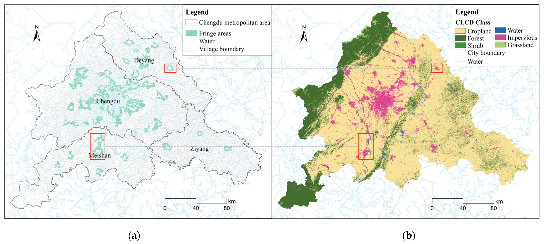
The sensitivity analysis showed that the 50% threshold provided the most balanced result between spatial integrity and the exclusion of marginally intersecting units (Appendix A Table A1). Based on POI kernel density and density–distance curves, the urban core boundaries and outer fringe boundaries of Chengdu, Deyang, Meishan, and Ziyang were identified separately. The area between the core boundary and the outer fringe boundary was defined as the metropolitan fringe area. The delineated fringe areas were distributed around the main urban cores but did not form regular concentric rings. Instead, they showed a combination of ring-shaped, semi-ring-shaped, corridor-extending, and node-embedded spatial forms.
Chengdu showed the most complex fringe structure, mainly distributed around the outer part of the central urban area, along Tianfu Avenue, near industrial parks, large residential clusters, and major transport nodes. Deyang’s fringe areas extended from the central urban area toward railways, expressways, and major roads. Meishan’s fringe areas were mainly distributed around the central urban area and along the corridor toward Chengdu. Ziyang’s fringe areas were concentrated around its central urban area and county-level nodes, showing a relatively clear spatial structure. After overlaying the delineated fringe areas with village-level administrative units, 786 village units were selected for analysis, including 516 in Chengdu, 142 in Deyang, 72 in Meishan, and 56 in Ziyang (Table 4).
The spatial validation results show that the delineated fringe areas were generally consistent with areas of impervious surface, especially around urban core edges, transport corridors, industrial parks, and residential expansion areas (Figure 3). In some local areas, the POI density-based delineation differed from the impervious surface. These differences were mainly observed around large residential communities, transport facilities, industrial spaces, and ecological spaces. These discrepancies suggest that POI density and impervious surface capture different aspects of fringe functions. POI density is more sensitive to formal facility agglomeration, whereas impervious surface better reflects the physical extent of residential development, transport infrastructure, and large-scale facilities.

3.2. Spatiotemporal Patterns of Fringe-Area Vitality

Urban vitality in the Chengdu Metropolitan Area showed a general gradient from urban cores to peripheral areas, but the gradient was neither uniform nor strictly monotonic. High-vitality units were mainly distributed around the outer edges of urban cores, county-level centers, major transport corridors, industrial parks, large residential clusters, and public-service nodes. Low-vitality units were mainly located in peripheral agricultural spaces, ecological protection areas, and low-density rural settlements.
In Chengdu, high-vitality fringe units were concentrated around the outer central urban area, the Tianfu Avenue corridor, industrial parks, and large residential groups. In Deyang, high-vitality units were mainly clustered around Jingyang District and its surrounding areas. In Meishan and Ziyang, high-vitality units were mainly distributed around urban center nodes and major transport corridors. Overall, fringe vitality showed a multi-core and irregular clustered pattern, with several secondary vitality nodes connected by road, rail, and rapid transport corridors.
The Moran’s I values of weekday and weekend vitality were 0.2303 and 0.2407, respectively, indicating significant spatial clustering (Table 5). The spatial patterns of weekday and weekend vitality were generally similar, but local differences were observed. The mean weekend vitality was slightly higher than the mean weekday vitality. Weekday high-vitality areas were mainly located near employment nodes, industrial parks, logistics spaces, public-service facilities, and commuting corridors, showing a production-oriented activity pattern. In contrast, weekend vitality showed a stronger life-oriented and recreation-oriented pattern, with higher values extending toward residential spillover areas, commercial consumption nodes, ecological recreation spaces, greenways, parks, and rural leisure areas.
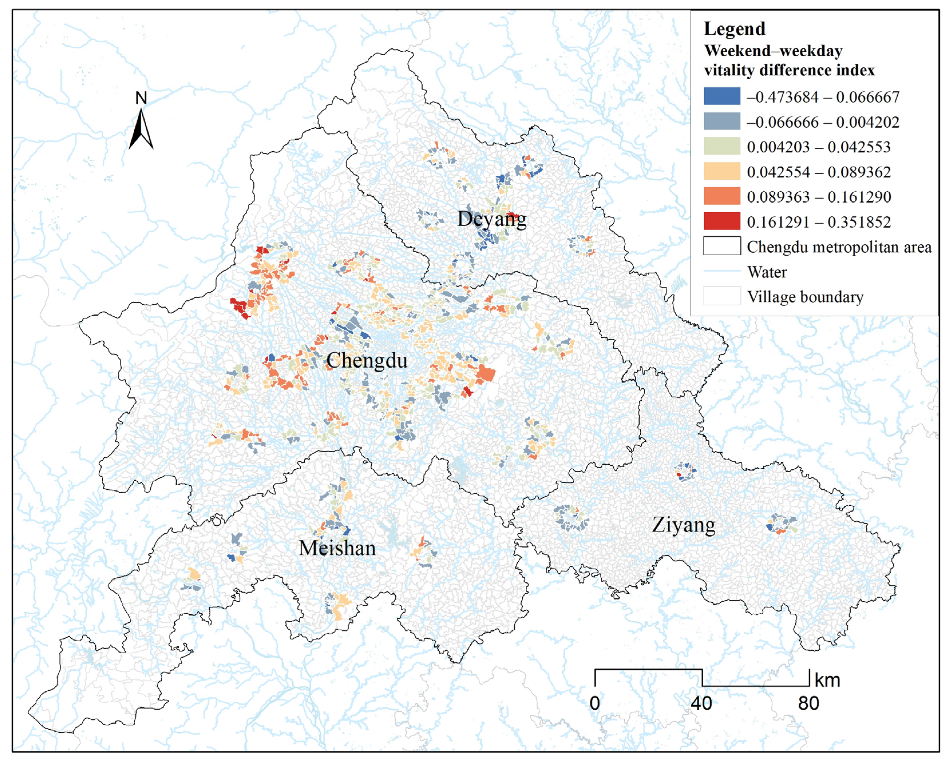
Areas with a relatively high weekend–weekday vitality difference index were mainly located in ecologically rich areas around the outer part of Chengdu and in several tourism and leisure nodes. Areas with an index greater than 0.04 included Dujiangyan and the Qingcheng Mountain scenic area in the northwest of Chengdu, ecological communities in the southern and southeastern parts of Chengdu, waterfront landscape areas, and Luodai Ancient Town. These areas are likely to be associated with stronger tourism, entertainment, and leisure-consumption activities during weekends (Figure 4).
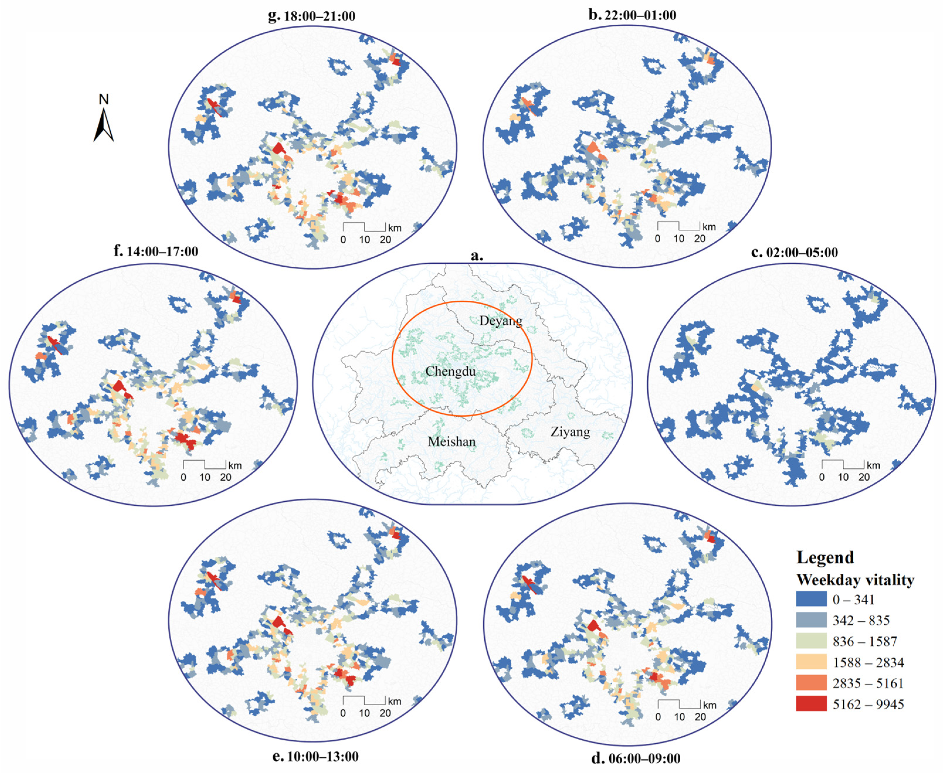
On weekdays, vitality began to increase at approximately 06:00, reached a relatively high level around 09:00, and remained high until approximately 18:00. High-vitality areas were mainly concentrated around the edges of urban cores, especially the high-tech industrial parks, the Longquan Economic and Technological Development Zone, and the Dujiangyan Binjiang tourism industrial functional area. This pattern is consistent with employment activity and commuting characteristics in fringe areas. From 18:00 to the early morning, vitality gradually decreased.
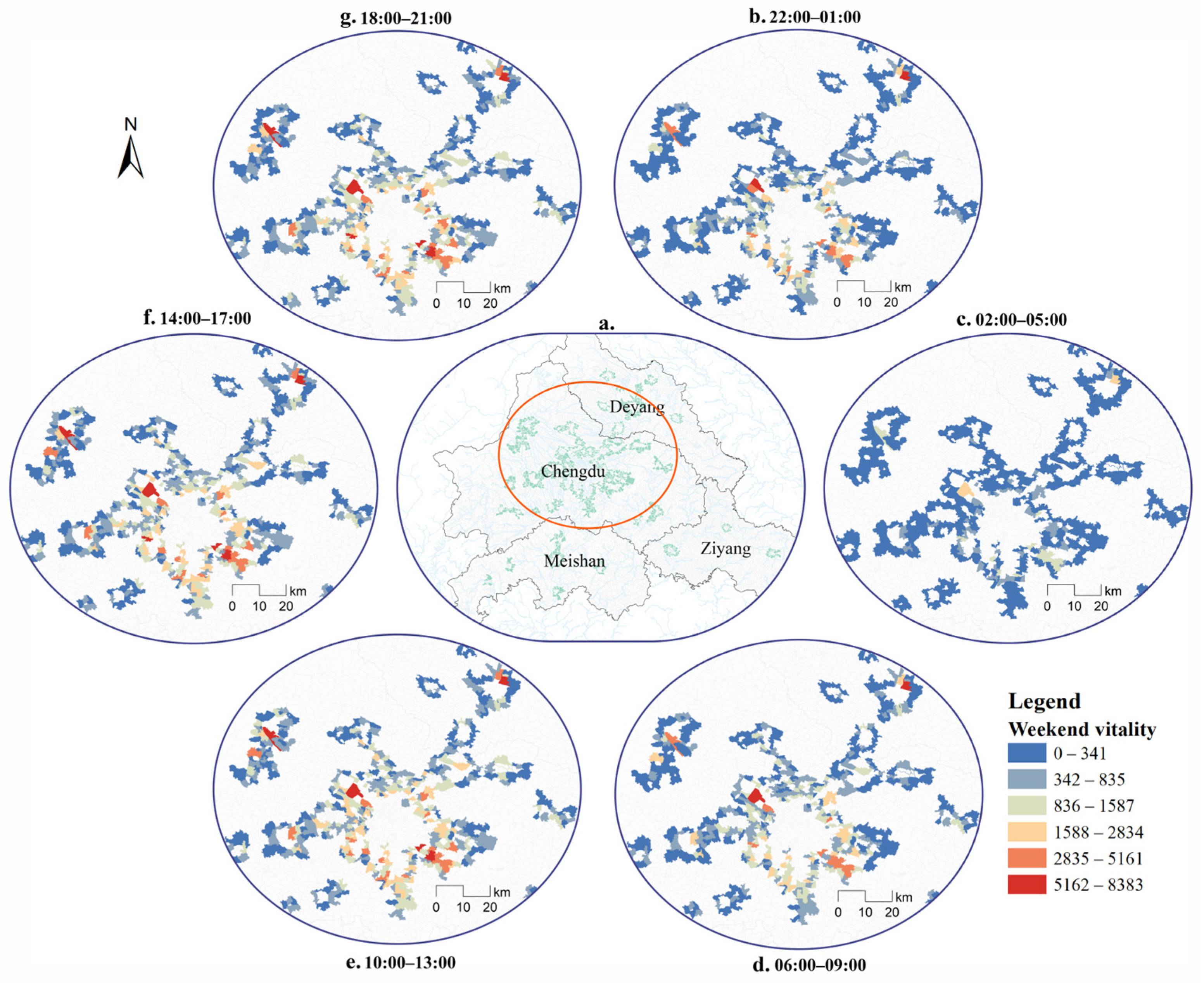
Compared with weekdays, weekend vitality showed weaker nighttime continuity. It increased gradually from 06:00 and remained at a relatively stable high level between 06:00 and 21:00, without the obvious commuting peak observed on weekdays. Some industrial parks and employment-oriented areas showed lower activity intensity on weekends, while ecological tourism areas, urban parks, waterfront spaces, and rural leisure areas became more active. For example, the Luxelakes Eco-City area, Nanhu Park, and several rural tourism nodes formed new weekend vitality hotspots. These patterns suggest that activity centers in fringe areas shift from production spaces to consumption, leisure, and ecological-experience spaces on weekends. After 21:00, weekend vitality gradually declined and reached a low level around midnight (Figure 5 and Figure 6).

3.3. An Interpretive Typology of Vitality Spaces in Metropolitan Fringe Areas

Based on observed spatial patterns, temporal differences, POI composition, and representative areas, this study proposes an exploratory interpretive typology of fringe vitality spaces. This typology is not a statistically validated classification and is not intended to assign every village unit to a mutually exclusive category. Rather, it provides a planning-oriented synthesis of the dominant functional sources and temporal rhythms of vitality in metropolitan fringe areas. Representative cases were first screened using weekday–weekend activity rhythms, POI composition, and built-environment indicators; high-resolution satellite imagery was used only as morphological corroboration. Five types were identified: industrial-production spaces, residential-spillover spaces, transport-corridor spaces, ecological-recreation spaces, and comprehensive-service spaces (Table 6).
Industrial-production spaces are mainly located around industrial parks, manufacturing bases, and logistics nodes. They show relatively high weekday vitality, and some areas maintain activity intensity during weekends. Residential-spillover spaces are mainly distributed in suburban residential clusters, rail-transit communities, and large living groups, where evening and weekend vitality is relatively prominent. Transport-corridor spaces are formed along expressways, arterial roads, railways, and transport stations, showing node-based or corridor-based vitality patterns. Ecological-recreation spaces are located near large parks, greenways, rural landscapes, and ecological resources, with stronger weekend or time-specific vitality. Comprehensive-service spaces are mainly distributed around universities, hospitals, public-service facilities, commercial nodes, and mixed residential areas, and show relatively stable vitality across weekdays and weekends.

3.4. Model Performance and Variable Importance

The LightGBM models showed substantially better predictive performance than the ordinary least squares baseline models for both weekday and weekend vitality. For weekday vitality, the LightGBM model achieved an R2 of 0.6888, a RMSE of 0.7446, and a MAE of 0.6027 on the testing set, whereas the ordinary least squares model achieved an R2 of 0.3884. For weekend vitality, the LightGBM model achieved an R2 of 0.7387, a RMSE of 0.6611, and a MAE of 0.5007, whereas the ordinary least squares model achieved an R2 of 0.4236 (Table 7). Under the current train–test split and cross-validation setting, the results suggest that the nonlinear LightGBM models achieved higher predictive accuracy than the linear OLS baseline in capturing associations between built-environment variables and fringe vitality.
The spatial-block cross-validation produced more conservative performance estimates than the random train–test split and random five-fold cross-validation, indicating that part of the predictive accuracy under random validation was associated with spatial proximity between training and validation observations. The Global Moran’s I values of the spatial-block out-of-fold residuals were 0.2908 for weekday vitality and 0.3766 for weekend vitality, both significant at p < 0.001. These results suggest that spatial blocking reduced spatial information leakage but did not eliminate residual spatial dependence. Accordingly, the model should be interpreted as providing reliable within-region predictive associations, while its cross-regional transferability remains to be further evaluated.
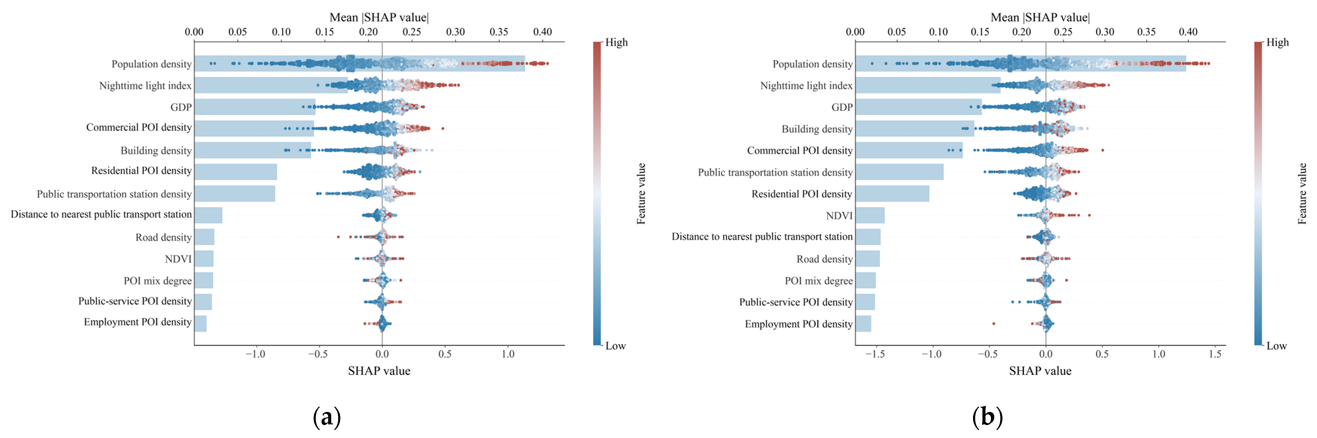
The SHAP-based variable-importance results show that population density, nighttime light, gross domestic product, building density, and commercial POI density made relatively large contributions to both weekday and weekend models (Table 8 and Figure 7). Population density had the largest mean absolute SHAP value in both models, reaching 0.3795 for weekdays and 0.3972 for weekends, indicating that population concentration remains a key predictor of fringe-area vitality. Nighttime light and gross domestic product also ranked high in both models, suggesting that socioeconomic activity and development level are closely associated with activity intensity. Building density and commercial POI density were also important, indicating that development intensity and commercial service provision are relevant to the formation of fringe vitality.
The ranking of variables differed slightly between weekday and weekend models. In the weekday model, commercial POI density ranked fourth and building density ranked fifth, whereas in the weekend model, building density ranked fourth and commercial POI density ranked fifth. This difference suggests that both development intensity and commercial services are important across time periods, but their relative contributions vary between production-oriented weekday activities and life-oriented weekend activities. Road density and distance to the nearest public transport station showed lower overall importance than the top five variables, but they still provide contextual information on transport-related activity patterns.

3.5. Nonlinear Built-Environment Associations and Saturation-like Patterns

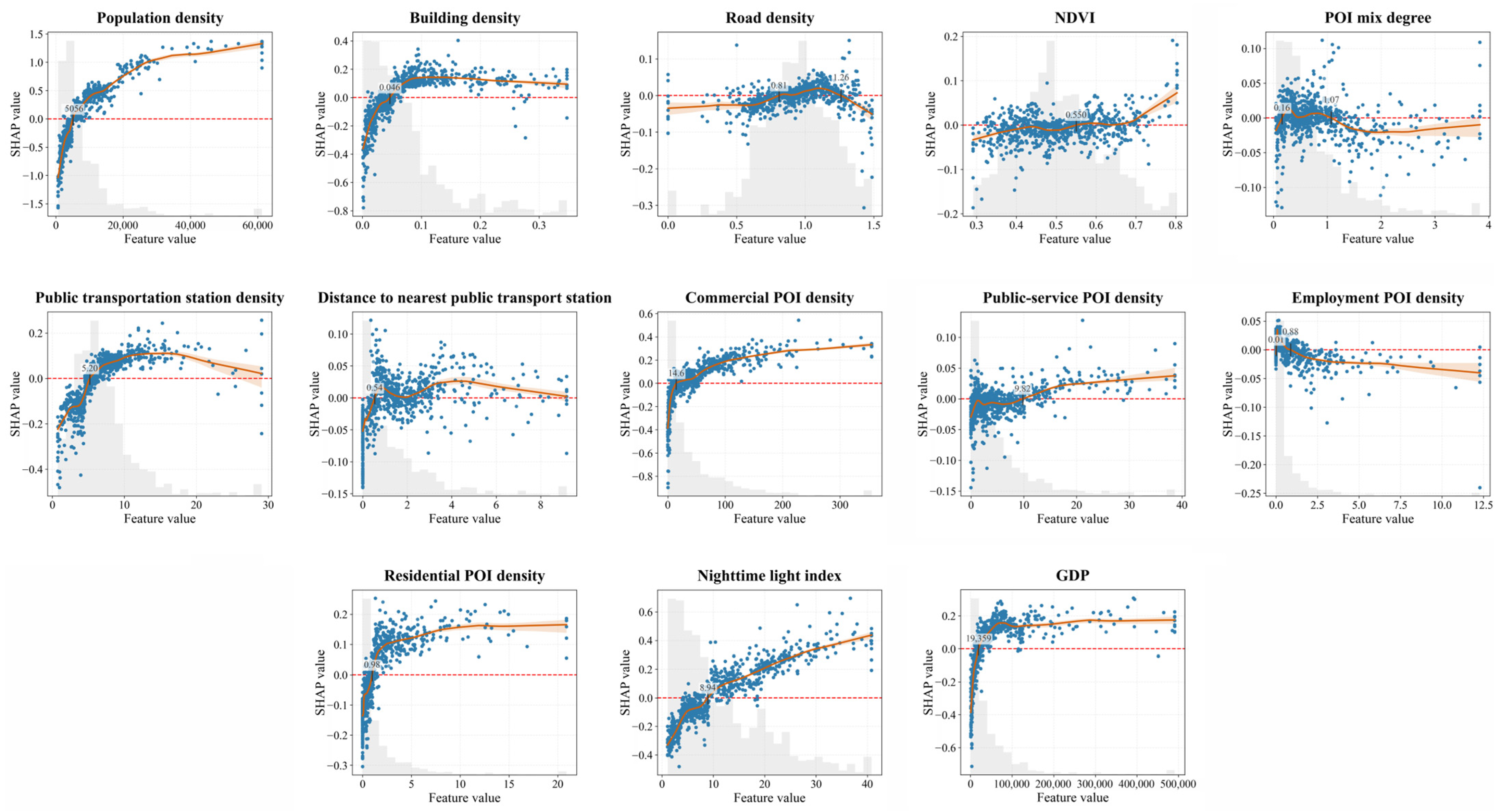
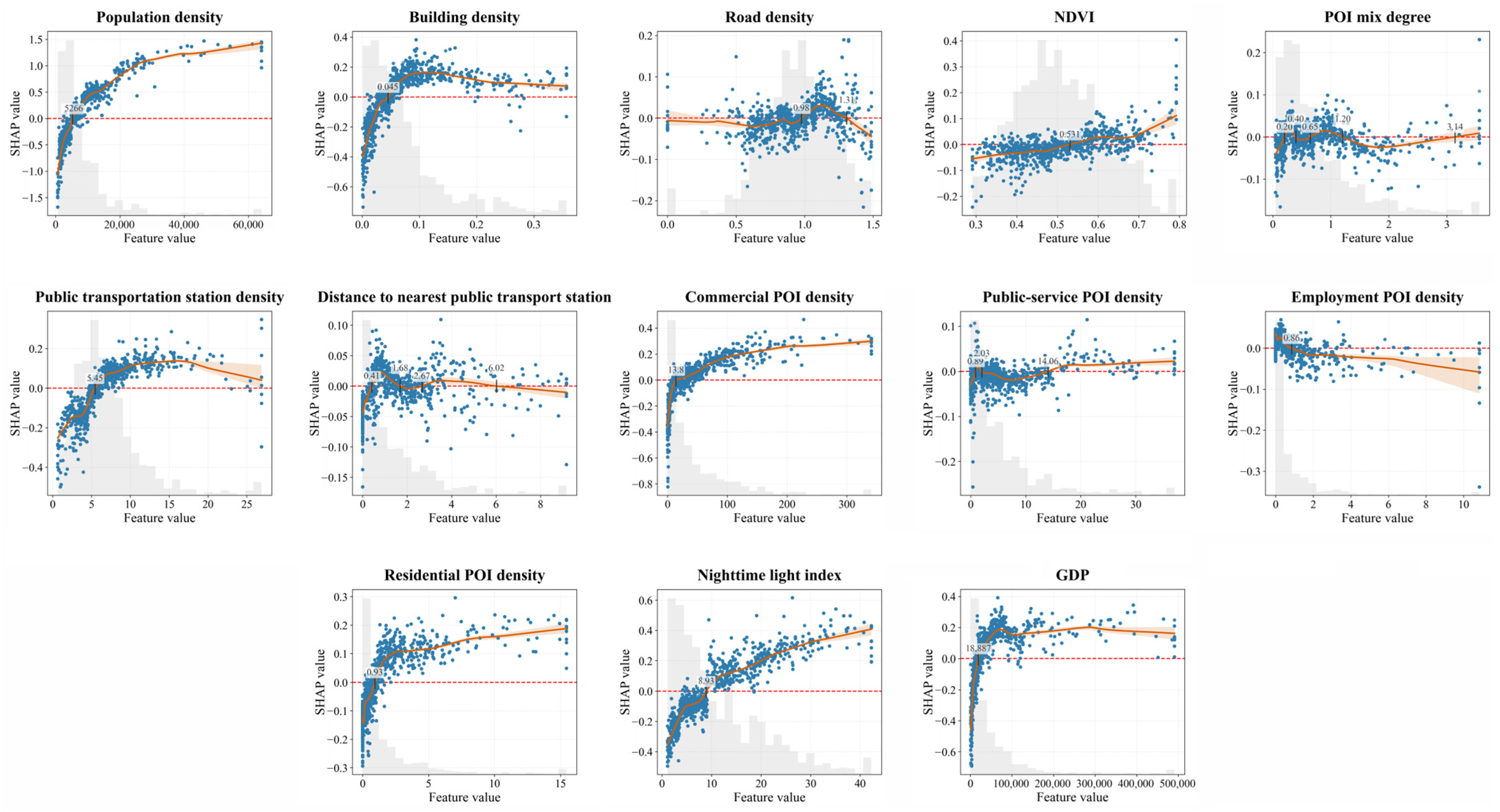
The SHAP dependence plots indicate that several built-environment variables had nonlinear associations with predicted fringe vitality (Figure 8 and Figure 9). The confidence bands were relatively narrow across the middle ranges of the principal predictors, where most observations were concentrated, but widened at the extreme high-value ranges. Therefore, the flattening patterns of population, building density, and commercial facilities were more stable within the main observed ranges, whereas apparent fluctuations at the distribution tails should be interpreted cautiously. The weekday and weekend models showed broadly similar patterns. For building density, SHAP values were close to zero or negative when the variable value was below an approximate threshold of 0.046 and became positive as building density increased. However, the positive contribution tended to level off at higher values, suggesting a saturation-like pattern rather than a continuously increasing effect. This result indicates that very low development intensity may be insufficient to support activity, but increasing building density beyond a certain range does not necessarily produce proportional gains in vitality.
Commercial POI density, nighttime light, and gross domestic product generally showed positive associations with predicted vitality. Their SHAP values increased rapidly at lower value ranges and then tended to flatten at higher ranges. This pattern suggests that a basic level of commercial service provision and socioeconomic activity is important for supporting fringe vitality, but additional increases may have diminishing marginal associations with activity intensity.
Other variables showed more context-dependent patterns. Road density did not exhibit a simple monotonic positive association, indicating that additional roads do not automatically translate into higher vitality. Public transport station density showed a generally positive but flattening association, whereas the distance to the nearest public transport station showed a non-monotonic pattern. Residential POI density was generally positively associated with vitality, while normalized difference vegetation index showed weak and partly positive associations, especially in the weekend model. POI functional mix showed a non-monotonic pattern, with relatively higher contributions at intermediate levels and weaker contributions at very low or very high levels.

4. Discussion

4.1. Metropolitan Fringe Vitality as a Product of Land-Use Transition

The spatial patterns suggest that vitality within the delineated fringe does not follow a uniform core–periphery gradient. Instead, high-vitality units are clustered around core-edge areas, transport corridors, industrial parks, residential groups, public-service nodes, and ecological recreation spaces. This finding is partly consistent with previous urban vitality studies that emphasize the roles of development intensity, commercial facilities, road connectivity, and functional mix [17,24]. However, the spatial expression of vitality in metropolitan fringe areas differs from the continuous street-based vitality commonly observed in central urban areas. Fringe vitality is more likely to appear as node-based, patch-based, and corridor-based activity clusters.
This difference suggests that fringe vitality should not be interpreted simply as a weakened extension of central-city vitality. Metropolitan fringe areas are formed through the reorganization of production, residence, transport, public services, ecological recreation, and rural functions during land-use transition [2,3]. This interpretation complements conventional approaches based on administrative boundaries or built-up land by highlighting the relational and transitional character of fringe space. Their mixed functions are therefore reflected not only in land-use morphology, but also in human activity patterns and temporal rhythms [2].
The weekday-weekend difference further reveals the temporal characteristics of fringe functions. Industrial-production spaces maintain relatively high activity intensity on weekdays, residential-spillover spaces become more active in the evening and on weekends, and ecological-recreation spaces show clear weekend enhancement [37]. In particular, activity in ecological and recreational areas may be more sensitive to tourism seasonality, weather conditions, holidays, and other short-term environmental factors. Previous studies on temporal variations in urban vitality have also suggested that single-time-point or daily average indicators may obscure the different activity rhythms of functional spaces [13,24]. Therefore, metropolitan fringe areas should not be understood simply as low-vitality peripheries, commuting hinterlands, or dormitory suburbs. They should instead be interpreted as land-use transition interfaces where production, residence, services, transport, and recreation overlap. This interpretation supplements morphological accounts of peri-urban transition by demonstrating that land-use heterogeneity is accompanied by differentiated activity performance and temporal rhythms. Metropolitan fringes are therefore not only zones where urban and rural land uses coexist, but also spaces where different functional systems generate uneven and time-specific forms of urbanity.

4.2. Nonlinear Associations and the Need for Sufficient Urbanity

The SHAP results indicate nonlinear and saturation-like associations between several built-environment variables and fringe vitality. This finding is consistent with recent studies that have shifted from linear correlations toward nonlinear interpretations of built environment-vitality relationships [26,27,28]. However, the present study extends this perspective to metropolitan fringe areas, where built-environment variables may have different meanings from those in compact central urban areas.
Building density provides an important example. In central urban areas, higher building density often reflects intensive development and concentrated functions [38]. In fringe areas, however, building density may first indicate whether basic spatial conditions for residence, employment, consumption, and services have been formed. The results suggest that low building density is associated with limited vitality, while higher building density is positively associated with higher predicted vitality up to a point and then shows a flattening pattern. This does not imply that fringe areas should pursue simple high-density development. In this study, sufficient urbanity refers to the joint presence of basic levels of population concentration, development intensity, service provision, transport accessibility, and socioeconomic activity that are sufficient to support everyday life in metropolitan fringe areas. The empirical basis for this interpretation lies in the nonlinear and saturation-like associations exhibited by several major predictors rather than directly tested causal mechanisms. We interpret the observed threshold and diminishing-return patterns as suggesting that vitality in fringe areas is more likely to emerge where several basic urban-support conditions coexist rather than where any single attribute is maximized. This interpretation remains theoretical and should be further examined using longitudinal data, interaction analyses, and comparative evidence from other metropolitan regions.
Commercial POI density, nighttime light, and gross domestic product show a similar logic. When commercial facilities are insufficient, fringe areas may lack the basic conditions for continuous consumption and service activities. Once commercial facilities and socioeconomic activity reach a certain level, vitality is strengthened, but further increases do not necessarily produce proportional gains. The strong contribution of nighttime light in both weekday and weekend models suggests that fringe vitality is related not only to daytime production and commuting activities, but also to residential life, nighttime consumption, and large-scale facility activity [25]. Therefore, the improvement of fringe vitality should not be based on copying high-intensity central-city development. It requires coordinated support from basic development intensity, service provision, transport linkage, and socioeconomic activity. This extends vitality research from the continuous street-life model commonly applied to central urban areas toward a node–corridor–patch interpretation suited to land-use transition contexts.
The study advances nonlinear built-environment research by showing that the relevance of density, accessibility, services, and socioeconomic activity depends on their observed levels and on the presence of complementary urban conditions. The findings therefore move the literature beyond identifying important predictors toward understanding stage-dependent marginal associations and the coordinated configuration of conditions supporting vitality.

4.3. Context-Dependent Meanings of Transport, Greenness, and Functional Mix

The results for transport variables suggest that the predictive association between accessibility and vitality in fringe areas may differ from that commonly observed in central urban areas. Central-city and transit-oriented development studies often emphasize the role of public transport proximity in attracting human activities [22,23]. In this study, however, road density and distance to the nearest public transport station did not show simple monotonic associations. This may be related to the greater dependence of fringe areas on expressways, logistics routes, parking conditions, and cross-district commuting. In fringe areas, transport infrastructure contributes to vitality only when it is effectively connected with residential groups, industrial parks, and public-service nodes.
Normalized difference vegetation index also has a context-dependent meaning. In some central urban studies, higher normalized difference vegetation index may be associated with lower construction intensity and therefore lower activity intensity [17,39]. In metropolitan fringe areas, however, green spaces, greenways, suburban parks, and rural recreation landscapes may become weekend destinations and support leisure consumption. Therefore, ecological space does not necessarily correspond to low predicted vitality; under suitable accessibility and service conditions, it may be associated with time-specific vitality, especially on weekends.
The non-monotonic association of POI functional mix suggests that more functional categories do not automatically produce higher vitality in fringe areas. Classical urban vitality theories emphasize the role of functional mix in increasing activity opportunities and extending the duration of space use [9,10]. However, in fringe areas, functional mix often occurs under conditions of uneven development, fragmented spatial form, and incomplete transport organization [1,4]. Moderate functional mix may support vitality, but very high mix without sufficient population scale, spatial coherence, and transport coordination may indicate fragmented or poorly organized functions.
This study does not reject the basic insights of central-city vitality research concerning density, functional mix, transport, and green space. Rather, it shows that these mechanisms may undergo scale transformation and contextual reconstruction in metropolitan fringe areas [17,22]. Fringe areas require sufficient urbanity to support activity, but they should not simply be transformed into central-city-like spaces. They require transport connections, but road construction alone does not necessarily generate vitality. They require ecological protection, but ecological spaces may also support leisure and consumption activities. The key issue in fringe vitality research is not only to identify important variables, but also to explain how and why their meanings change in land-use transition contexts.

4.4. Planning Implications

Metropolitan fringes in different countries commonly experience fragmented land development, functional separation, infrastructure-led growth, and uneven service provision. Under such conditions, vitality may similarly emerge through discontinuous nodes, corridors, and patches rather than decline uniformly with distance from the urban core. Thus, the specific numerical relationships are context-dependent, whereas the broader emphasis on functional coordination, development stage, and diminishing predictive returns may be applicable to other metropolitan fringe areas. Comparative studies across different planning systems and urbanization trajectories are needed to evaluate this proposition.
These findings have several planning implications. First, metropolitan fringe areas should not be governed by a single logic of either urban expansion or ecological protection. Different fringe spaces have different sources of vitality and therefore require differentiated planning strategies [40]. For industrial-production spaces, a concentration of industrial functions alone may create a mismatch between employment locations and everyday services. Therefore, planning should not focus solely on expanding industrial land, but should instead promote the transformation of industrial areas into mixed-use employment communities. Planning may need to coordinate industrial land with daily services, public transport connections, and public spaces to reduce the commuting costs associated with jobs–housing separation and improve the efficiency of space use outside weekday working hours. For residential-spillover spaces, housing-led expansion should be avoided where commercial services, education, healthcare, public transport, and pedestrian facilities remain inadequate, so as to prevent the formation of dormitory towns. Planning should focus on improving local living circles by supplementing education, healthcare, commercial services, and public activity spaces, while optimizing bus routes, strengthening walking and cycling networks, and enhancing community public spaces to improve the convenience of residents’ daily activities and their engagement with local environments. The findings also indicate that transport infrastructure alone does not automatically generate spatial vitality. Agglomeration effects can emerge only when transport corridors are effectively connected with employment, residential, and service nodes. Therefore, future transport planning in metropolitan fringe areas should avoid relying solely on rapid corridors or linear development. Instead, mixed-use development should be promoted around transport nodes, with coordinated provision of public services, commercial spaces, and employment opportunities to translate transport advantages into spatial vitality.
Ecological-recreation spaces provide a different pathway for fringe vitality. Parks, greenways, suburban landscapes, and rural tourism resources may generate weekend activity clusters, but this does not justify high-intensity commercial development. A more appropriate strategy is to maintain ecological protection while improving greenway systems, walking and cycling facilities, public transport connections, and basic service infrastructure to enhance the accessibility and effective use of ecological resources. Overall, improving fringe vitality requires coordinated land-use, transport, service, and ecological planning rather than reliance on a single density or infrastructure indicator. The differentiated planning approach proposed in this study emphasizes a shift from spatial expansion to functional coordination and from the intensification of individual elements to the creation of integrated supporting conditions, thereby providing a spatial basis for the fine-grained governance of metropolitan fringe areas under rapid urbanization.

4.5. Limitations and Future Research

This study has several limitations. First, the observation period covered one non-holiday week in July 2023, which may not fully capture seasonal variations or long-term vitality patterns. Baidu heatmap data also represent relative activity intensity rather than actual population counts, and the results may be affected by platform-user structure and data-generation mechanisms [24]. Second, the cross-sectional variables used in this study cannot reveal the temporal processes, direction, or rate associated with land-use change. Future research should integrate longitudinal activity observations to examine how the formation and evolution of these interfaces are associated with changes in metropolitan-fringe vitality. Third, village-level administrative units are useful for planning interpretation but may introduce the modifiable areal unit problem [41]. Although spatial-block cross-validation was conducted to reduce spatial information leakage, significant residual spatial autocorrelation remained. Future research should further explore spatial modeling approaches and multi-city comparisons to improve the assessment of model transferability. Fourth, POI kernel density is sensitive to formal facility agglomeration and may underestimate low-intensity residential activities, agricultural production, ecological recreation, or informal activities. Finally, LightGBM and SHAP identify predictive associations and variable contributions, not strict causal effects.
Future research could combine mobile-phone signaling, public transport smart-card records, long-term remote sensing data, travel surveys, and causal-inference methods to further examine the long-term dynamics and mechanisms of fringe vitality. Comparative studies across multiple metropolitan areas would also help test whether the vitality typology and the idea of sufficient urbanity identified in this study are transferable to other urban-rural transition contexts.

5. Conclusions

This study examined urban vitality in metropolitan fringe areas of the Chengdu Metropolitan Area by integrating POI-based fringe delineation, Baidu heatmap-based vitality measurement, built-environment indicators, LightGBM modeling, and SHAP interpretation. The results show that metropolitan fringe areas are not homogeneous low-vitality peripheries. Instead, they contain clustered vitality nodes around urban core edges, transport corridors, industrial parks, residential spillover areas, public-service nodes, and ecological recreation spaces. Fringe vitality also differs between weekdays and weekends, reflecting the combined influence of production, residence, commuting, services, and recreation.
The modeling results indicate that population density, nighttime light, gross domestic product, building density, and commercial POI density show the highest SHAP-based predictive contributions in both weekday and weekend models. Several variables show nonlinear and saturation-like associations, while transport, greenness, and functional mix show more context-dependent patterns. These results suggest that vitality in metropolitan fringe areas should not be understood as a simple linear extension of central-city vitality. Rather, it is associated with a sufficient level of population concentration, development intensity, service provision, transport linkage, and socioeconomic activity, together with functional coordination and land use-transport matching.
By extending urban vitality research to metropolitan fringe areas, this study provides empirical evidence for understanding land-use transition interfaces in rapidly urbanizing metropolitan regions. This extends vitality research from the continuous street-life model commonly applied to central urban areas toward a node–corridor–patch interpretation suited to land-use transition contexts. It also moves beyond the conventional center–periphery perspective by conceptualizing metropolitan-fringe vitality as a heterogeneous spatial phenomenon composed of multiple functional vitality configurations rather than a uniformly declining urban periphery. The findings also suggest that vitality enhancement depends on the coordinated provision of urban conditions rather than the maximization of individual attributes. Fringe-area planning should adopt differentiated strategies according to industrial-production, residential-spillover, transport-corridor, ecological-recreation, and comprehensive-service contexts.

Author Contributions

Conceptualization, Y.J.; methodology, Y.J. and Q.Y.; software, L.Z.; validation, B.H.; formal analysis, Y.J. and L.Z.; investigation, Q.Y.; resources, B.H.; data curation, L.Z.; writing—original draft preparation, L.Z. and Q.Y.; writing—review and editing, Y.J., H.Y. and J.C.; visualization, L.Z.; supervision, Y.J. and B.H.; project administration, B.H.; funding acquisition, Y.J. All authors have read and agreed to the published version of the manuscript.

Funding

This study was supported by the National Natural Science Foundation of China (No. 52508086), the Special Research Project on Chengdu Metropolitan Area Construction of the Chengdu Philosophy and Social Science Planning Project (No. 2025ZX01), Natural Science Foundation of Sichuan Province (No. 2026NSFSC1300; No. 2026NSFSC1302), and Fundamental Research Funds for the Central Universities (No. 2682026CX048, No. 2682025CX123).

Data Availability Statement

The study uses public and third-party spatial datasets. Public datasets are available from the original data providers cited in the manuscript. Restrictions apply to Amap POI data and Baidu heatmap data because they are third-party datasets. Processed village-level indicators and model outputs are available from the corresponding author upon reasonable request, subject to the terms and conditions of the original data providers.

Conflicts of Interest

The authors declare no conflicts of interest.

Appendix A

Appendix A.1. Thresholds for Fringe-Area Delineation

To support the identification of kernel density thresholds used in delineating metropolitan fringe areas, this study constructed POI density-equivalent radius curves and density-expansion increment curves for Chengdu, Deyang, Meishan, and Ziyang. The equivalent expansion radius was obtained by converting the area enclosed by each POI density contour into the radius of an equal-area circle. The expansion increment represents the change in equivalent expansion radius between adjacent density thresholds and was used to identify stage changes in spatial expansion. The final threshold selection was based on the combined interpretation of the two curves, impervious surface, remote sensing imagery, road-network patterns, and actual spatial conditions (Appendix A Figure A1, Figure A2, Figure A3 and Figure A4).
Figure A1. POI kernel density and density–distance curves in Chengdu: (a) density–equivalent radius curve; (b) density–expansion increment curve.
Land 15 01380 g0a1
Figure A2. POI kernel density and density–distance curves in Deyang: (a) density–equivalent radius curve; (b) density–expansion increment curve.
Land 15 01380 g0a2
Figure A3. POI kernel density and density–distance curves in Meishan: (a) density–equivalent radius curve; (b) density–expansion increment curve.
Land 15 01380 g0a3
Figure A4. POI kernel density and density–distance curves in Ziyang: (a) density–equivalent radius curve; (b) density–expansion increment curve.
Land 15 01380 g0a4
To examine the sensitivity of the village-unit selection to the overlap criterion, five alternative threshold scenarios, ranging from 30% to 70%, were constructed. The metropolitan fringe at the village-unit level was identified based on the proportion of each village overlapping the fringe polygon delineated by the selected kernel-density isolines. The selected village units were subsequently overlaid with land-use data to calculate the area and share of built-up land within the identified fringe. The results indicate that the 50% scenario represents a stabilization point. Compared with the 60% scenario, it substantially improves the spatial continuity of the identified fringe, reducing the number of disconnected components from 47 to 31. Below 50%, increases in total area and built-up land are limited, while the built-up land proportion remains almost unchanged.
The 50% threshold was therefore retained because it ensures that the delineated fringe constitutes the dominant spatial context of each selected village, while excluding villages that only marginally intersect the fringe-isoline boundary.
Table A1. Sensitivity of the village-based metropolitan fringe extent to alternative overlap-threshold scenarios.
Threshold
Scenario
Number of
Selected Village Units
Total Area of
Dissolved Village Polygons (km2)
Built-Up Land Area (km2)Share of Built-Up Land (%)Number of
Spatially Connected Components
70%5401704.74461.3827.0658
60%6392201.40537.8424.4347
50%7862947.60657.1522.4831
40%8612983.96669.1722.4332
30%8833042.47678.7322.3132

Appendix A.2. Model Robustness Test

Table A2 compares the full model (M0) with three reduced specifications: M1 excludes the nighttime light index, M2 excludes GDP, and M3 excludes POI mix degree, commercial POI density, public-service POI density, employment POI density, and residential POI density. Random five-fold cross-validation performance remained nearly identical across the four models. Under the more stringent spatial-block cross-validation, M0 achieved the best overall performance for both weekday and weekend vitality. For weekday vitality, the spatial-block R 2 of M0 was 0.5112, compared with 0.4994, 0.4794, and 0.5047 for M1–M3, respectively. For weekend vitality, the corresponding values were 0.5314, 0.5031, 0.5059, and 0.5195. M0 also produced the lowest spatial-block RMSE, MAE, and residual Moran’s I . The overall comparison indicates that the predictive performance and principal conclusions are not driven solely by nighttime light, GDP, or POI-derived variables, supporting the use of M0 as the primary model.
Table A2. Robustness checks using alternative variable specifications.
TimeModelRandom 5-Fold CVSpatial-Block CVSpatial Residual Moran’s Ip-Value
R 2 RMSEMAE R 2 RMSEMAE
WeekdayM00.68880.74460.60270.51120.93250.75340.2908<0.001
M10.68870.74470.60340.49940.94370.76380.3073<0.001
M20.68910.74430.60290.47940.96230.77340.3308<0.001
M30.68890.74460.60380.50470.93870.75730.2972<0.001
WeekendM00.73870.66110.50070.53140.88940.70450.3766<0.001
M10.73860.66110.50070.50310.91590.72610.4111<0.001
M20.73860.66120.50090.50590.91330.72220.4051<0.001
M30.73860.66120.50050.51950.90070.70960.3886<0.001

References

  1. Ravetz, J.; Sahana, M. Where is the peri-urban? Mapping the areas ‘around, beyond and between’. Front. Sustain. Cities 2025, 7, 1436287. [Google Scholar] [CrossRef] [Scilit]
  2. Follmann, A.; Kennedy, L.; Pfeffer, K.; Wu, F. Peri-urban transformation in the Global South: A comparative socio-spatial analytics approach. Reg. Stud. 2023, 57, 447–461. [Google Scholar] [CrossRef] [Scilit]
  3. Pino, A.; Martínez, J.; Alfaro, M. Criteria for the Delimitation of the Urban Fringe of Latin American Cities: A Review from the Global South. Land 2025, 14, 1276. [Google Scholar] [CrossRef] [Scilit]
  4. Gonçalves, J.; Gomes, M.C.; Ezequiel, S.; Moreira, F.; Loupa-Ramos, I. Differentiating peri-urban areas: A transdisciplinary approach towards a typology. Land Use Policy 2017, 63, 331–341. [Google Scholar] [CrossRef] [Scilit]
  5. López-Goyburu, P.; García-Montero, L.G. The urban-rural interface as an area with characteristics of its own in urban planning: A review. Sustain. Cities Soc. 2018, 43, 157–165. [Google Scholar] [CrossRef] [Scilit]
  6. Dong, Q.; Qu, S.; Qin, J.; Yi, D.; Liu, Y.; Zhang, J. A method to identify urban fringe area based on the industry density of POI. ISPRS Int. J. Geo-Inf. 2022, 11, 128. [Google Scholar] [CrossRef] [Scilit]
  7. Yu, J.; Meng, Y.; Zhou, S.; Zeng, H.; Li, M.; Chen, Z.; Nie, Y. Research on Spatial Delineation Method of Urban-Rural Fringe Combining POI and Nighttime Light Data-Taking Wuhan City as an Example. Int. J. Environ. Res. Public Health 2023, 20, 4395. [Google Scholar] [CrossRef] [Scilit] [PubMed]
  8. Scott, A.J.; Carter, C.; Reed, M.R.; Larkham, P.; Adams, D.; Morton, N.; Waters, R.; Collier, D.; Crean, C.; Curzon, R.; et al. Disintegrated development at the rural–urban fringe: Re-connecting spatial planning theory and practice. Prog. Plan. 2013, 83, 1–52. [Google Scholar] [CrossRef] [Scilit]
  9. Jacobs, J. The Death and Life of Great American Cities; Random House: New York, NY, USA, 1961. [Google Scholar]
  10. Montgomery, J. Making a city: Urbanity, vitality and urban design. J. Urban Des. 1998, 3, 93–116. [Google Scholar] [CrossRef] [Scilit]
  11. Ye, Y.; Li, D.; Liu, X. How block density and typology affect urban vitality: An exploratory analysis in Shenzhen, China. Urban Geogr. 2018, 39, 631–652. [Google Scholar] [CrossRef] [Scilit]
  12. Gehl, J. Life Between Buildings: Using Public Space; Island Press: Washington, DC, USA, 2011. [Google Scholar] [CrossRef] [Scilit]
  13. De Nadai, M.; Staiano, J.; Larcher, R.; Sebe, N.; Quercia, D.; Lepri, B. The death and life of great Italian cities: A mobile phone data perspective. In Proceedings of the 25th International Conference on World Wide Web, Montreal, QC, Canada, 11–15 April 2016; International World Wide Web Conferences Steering Committee: Geneva, Switzerland, 2016; pp. 413–423. [Google Scholar] [CrossRef] [Scilit]
  14. Wu, C.; Ye, X.; Ren, F.; Du, Q. Check-in behaviour and spatio-temporal vibrancy: An exploratory analysis in Shenzhen, China. Cities 2018, 77, 104–116. [Google Scholar] [CrossRef] [Scilit]
  15. Chen, T.; Hui, E.C.M.; Wu, J.; Lang, W.; Li, X. Identifying urban spatial structure and urban vibrancy in highly dense cities using georeferenced social media data. Habitat Int. 2019, 89, 102005. [Google Scholar] [CrossRef] [Scilit]
  16. Xia, C.; Yeh, A.G.O.; Zhang, A. Analyzing spatial relationships between urban land use intensity and urban vitality at street block level: A case study of five Chinese megacities. Landsc. Urban Plan. 2020, 193, 103669. [Google Scholar] [CrossRef] [Scilit]
  17. Li, X.; Li, Y.; Jia, T.; Zhou, L.; Hijazi, I.H. The six dimensions of built environment on urban vitality: Fusion evidence from multi-source data. Cities 2022, 121, 103482. [Google Scholar] [CrossRef] [Scilit]
  18. Chen, Y.; Yu, B.; Shu, B.; Yang, L.; Wang, R. Exploring the spatiotemporal patterns and correlates of urban vitality: Temporal and spatial heterogeneity. Sustain. Cities Soc. 2023, 91, 104440. [Google Scholar] [CrossRef] [Scilit]
  19. Jiang, Y.; Sun, Z.; Wei, D.; Zhao, P.; Yang, L.; Lu, Y. Revealing the spatiotemporal pattern of urban vibrancy at the urban agglomeration scale: Evidence from the Pearl River Delta, China. Appl. Geogr. 2025, 181, 103694. [Google Scholar] [CrossRef] [Scilit]
  20. Zhang, A.; Li, W.; Wu, J.; Lin, J.; Chu, J.; Xia, C. How can the urban landscape affect urban vitality at the street block level? A case study of 15 metropolises in China. Environ. Plan. B Urban Anal. City Sci. 2020, 48, 1245–1262. [Google Scholar] [CrossRef] [Scilit]
  21. Rui, J.; Li, X. Decoding vibrant neighborhoods: Disparities between formal neighborhoods and urban villages in eye-level perceptions and physical environment. Sustain. Cities Soc. 2024, 101, 105122. [Google Scholar] [CrossRef] [Scilit]
  22. Cervero, R.; Kockelman, K. Travel demand and the 3Ds: Density, diversity, and design. Transp. Res. Part D Transp. Environ. 1997, 2, 199–219. [Google Scholar] [CrossRef] [Scilit]
  23. Ewing, R.; Cervero, R. Travel and the built environment: A meta-analysis. J. Am. Plan. Assoc. 2010, 76, 265–294. [Google Scholar] [CrossRef] [Scilit]
  24. Lv, G.; Zheng, S.; Hu, W. Exploring the relationship between the built environment and block vitality based on multi-source big data: An analysis in Shenzhen, China. Geomat. Nat. Hazards Risk 2022, 13, 1593–1613. [Google Scholar] [CrossRef] [Scilit]
  25. Mellander, C.; Lobo, J.; Stolarick, K.; Matheson, Z. Night-time light data: A good proxy measure for economic activity? PLoS ONE 2015, 10, e0139779. [Google Scholar] [CrossRef] [Scilit] [PubMed]
  26. Liu, D.; Lu, Y.; Yang, L. Exploring non-linear effects of environmental factors on the volume of pedestrians of different ages using street view images and computer vision technology. Travel Behav. Soc. 2024, 36, 100814. [Google Scholar] [CrossRef] [Scilit]
  27. Li, C.; Zhou, Y.; Wu, M.; Xu, J.; Fu, X. Exploring nonlinear threshold effects and interactions between built environment and urban vitality at the block level using machine learning. Land 2025, 14, 1232. [Google Scholar] [CrossRef] [Scilit]
  28. Lyu, G.; Angkawisittpan, N.; Fu, X.; Sonasang, S. Investigating the relationship between built environment and urban vitality using big data. Sci. Rep. 2025, 15, 579. [Google Scholar] [CrossRef] [Scilit] [PubMed]
  29. Ke, G.; Meng, Q.; Finley, T.; Wang, T.; Chen, W.; Ma, W.; Ye, Q.; Liu, T.-Y. LightGBM: A highly efficient gradient boosting decision tree. Adv. Neural Inf. Process. Syst. 2017, 30. [Google Scholar]
  30. Shao, J.; Long, Y.; Liu, X.; Zheng, Y.; Song, Y.; Wang, J.; Liu, B.; Yang, J.; Chen, Y.; Zhang, F. Machine learning-based study on factors influencing street vitality in urban fringe commercial districts: A case of Wuhan. Front. Archit. Res. 2026, 15, 582–608. [Google Scholar] [CrossRef] [Scilit]
  31. Lundberg, S.M.; Lee, S.-I. A unified approach to interpreting model predictions. In Proceedings of the 31st International Conference on Neural Information Processing Systems (NIPS’17); Curran Associates Inc.: Red Hook, NY, USA, 2017; pp. 4768–4777. [Google Scholar]
  32. Wolch, J.R.; Byrne, J.; Newell, J.P. Urban green space, public health, and environmental justice: The challenge of making cities ‘just green enough’. Landsc. Urban Plan. 2014, 125, 234–244. [Google Scholar] [CrossRef] [Scilit]
  33. National Development and Reform Commission of the People’s Republic of China. Chengdu Metropolitan Area Development Plan; National Development and Reform Commission: Beijing, China, 2022. Available online: https://www.ndrc.gov.cn/xwdt/ztzl/xxczhjs/ghzc/202203/P020220310612774783269.pdf (accessed on 16 June 2026).
  34. Liu, Y.; Jiang, B. Research on the Development of Medium-sized Cities from the Perspective of a Metropolitan Area—A Case Study of Ziyang City in the Chengdu Metropolitan Area. Int. J. Environ. Sustain. Prot. 2022, 2, 1–10. [Google Scholar] [CrossRef] [Scilit]
  35. Shannon, C.E. A mathematical theory of communication. Bell Syst. Tech. J. 1948, 27, 379–423. [Google Scholar] [CrossRef] [Scilit]
  36. Peng, J.; Zhao, S.; Liu, Y.; Tian, L. Identifying the urban-rural fringe using wavelet transform and kernel density estimation: A case study in Beijing City, China. Environ. Model. Softw. 2016, 83, 286–302. [Google Scholar] [CrossRef] [Scilit]
  37. Tang, S.; Ta, N. How the built environment affects the spatiotemporal pattern of urban vitality: A comparison among different urban functional areas. Comput. Urban Sci. 2022, 2, 39. [Google Scholar] [CrossRef] [Scilit] [PubMed]
  38. Xu, N.; Wang, P. Rethinking the relationship between ecological conservation and urban land development: A spatial–machine learning integration approach. Habitat Int. 2026, 171, 103755. [Google Scholar] [CrossRef] [Scilit]
  39. Jiang, Y.; Liu, D.; Ren, L.; Grekousis, G.; Lu, Y. Tree abundance, species richness, or species mix? Exploring the relationship between features of urban street trees and pedestrian volume in Jinan, China. Urban For. Urban Green. 2024, 95, 128294. [Google Scholar] [CrossRef] [Scilit]
  40. Shlomo, O. Segregated urbanization: Urban-rural bordering in the Tel Aviv metropolitan fringe. Cities 2026, 175, 107090. [Google Scholar] [CrossRef] [Scilit]
  41. Openshaw, S. The Modifiable Areal Unit Problem; Geo Books: Norwich, UK, 1983. [Google Scholar]
Figure 1. Location of the Chengdu Metropolitan Area.
Land 15 01380 g001
Figure 2. Framework diagram.
Land 15 01380 g002
Figure 3. Spatial validation of the delineated metropolitan fringe areas: (a) delineated fringe areas; (b) impervious-surface and land-cover distribution.
Land 15 01380 g003
Figure 4. Weekend–weekday vitality difference index.
Land 15 01380 g004
Figure 5. Weekday vitality pattern: (a) fringe area, the orange circle in panel (a) indicates the local core area of the metropolitan area; (bg) vitality distribution by 4 h time interval.
Land 15 01380 g005
Figure 6. Weekend vitality pattern: (a) fringe area, the orange circle in panel (a) indicates the local core area of the metropolitan area; (bg) vitality distribution by 4 h time interval.
Land 15 01380 g006
Figure 7. SHAP variable importance for weekday and weekend models: (a) weekday model; (b) weekend model.
Land 15 01380 g007
Figure 8. SHAP dependence plots of weekday vitality.
Land 15 01380 g008
Figure 9. SHAP dependence plots of weekend vitality.
Land 15 01380 g009
Table 1. Data sources and preprocessing.
TypeVariableData SourceTimeMeasurementInterpretation
VitalityUrban vitalityBaidu heatmap (http://rq.baidu.com/, accessed on 15 February 2026); 200 m × 200 m raster data10 July 2023–16 July 2023; hourlyArea-weighted aggregation of intersecting raster cells to village-level unitsReflects real-time urban activity intensity
DensityPopulation densityWorldPop: https://hub.worldpop.org/doi/10.5258/SOTON/WP00839 (accessed on 15 February 2026); 100 m × 100 m2024Total population within unit/unit area, person/km2Reflects population base
Building densityZenodo database: https://zenodo.org/records/8174931 (accessed on 15 February 2026)22 July 2023Building footprint area/unit areaReflects development intensity
Design and ecological backgroundRoad densityOpenStreetMap (https://www.openstreetmap.org/, accessed on 15 February 2026)1 January 2024Road length within unit/unit area, km/km2Reflects road-network connectivity and corridor linkage
NDVIUSGS EarthExplorer, Landsat 8 OLI/TIRS (https://earthexplorer.usgs.gov/, accessed on 15 February 2026)2024Landsat 8 imagery was used to calculate the Normalized Difference Vegetation Index (NDVI)Reflects vegetation cover level
DiversityPOI mix degreeAmap POI data (https://www.amap.com/, accessed on 15 February 2026)1 January 2024Shannon diversity index of POI categoriesReflects functional mixture and diversity
Public transport accessibilityPublic transportation station densityAmap POI data (https://www.amap.com/, accessed on 15 February 2026); bus and metro stations2024Number of stations within unit area, stations/km2Reflects public transport station supply
Distance to nearest public transport stationAmap POI data (https://www.amap.com/, accessed on 15 February 2026); bus and metro stations2024Euclidean distance from village-unit centroid to nearest stationReflects public transport proximity
Destination accessibilityCommercial POI densityAmap POI data (business, shopping, finance, catering, etc.)1 January 2024Business POI count within unit areaReflects concentration of commercial activity
Public-service POI densityAmap POI data (public service facilities)1 January 2024Public-service POI count within unit areaReflects concentration of public-service facilities
Employment POI densityAmap POI data (employment and work-related facilities)1 January 2024Employment POI count within unit areaReflects concentration of employment and work facilities
Residential POI densityAmap POI data (residential facilities)1 January 2024Residential POI count within unit areaReflects residential function
Socioeconomic backgroundNighttime light indexNPP-VIIRS Nighttime Light Dataset (https://eogdata.mines.edu/, accessed on 15 February 2026)2023Mean nighttime light value within unitReflects economic activity level
GDPChinese Academy of Sciences Resource and Environmental Science Data Center (https://www.resdc.cn/, accessed on 15 February 2026); 1 km × 1 km grid2023Mean GDP grid value within unitReflects economic development level
Table 2. Data used in the vitality assessment.
TypeTimeTime HorizonTime Interval
Weekday vitality10 July 2023–14 July 202324 h1 h
Weekend vitality15 July 2023–16 July 202324 h1 h
Table 3. Optimized Model Parameters.
ModelN_EstimatorsMax_DepthNum_LeavesSubsampleRandom Seed
Weekday779121140.822842
Weekend11068630.885842
Table 4. Statistics of delineated fringe areas by city.
CityFringe Area/km2Share of Total Fringe Area (%)Village UnitsMean POI Density (POIs/km2)
Chengdu2034.01369.005851653.5734
Deyang435.818114.785514252.9303
Meishan326.441911.07497229.4876
Ziyang151.32325.133885639.4916
Total2947.5965100786-
Table 5. Descriptive statistics of vitality indicators.
IndicatorMeanSDMinMaxMoran’s IZ Value p Value
Weekday vitality118.2824175.5027017010.230310.2040<0.01
Weekend vitality124.8779182.6978016680.240710.6439<0.01
Weekend–weekday vitality difference index0.02960.0645−0.47370.35190.300513.123<0.01
Table 6. Interpretive typology of vitality spaces in metropolitan fringe areas.
TypeIdentification BasisTemporal RhythmLand-Use ContextPlanning ConcernRepresentative
Example
Industrial-productionEmployment/industrial POI, weekday high vitalityweekday highindustrial parks, logistics basesjobs-housing-service mismatchLand 15 01380 i001
Residential-spilloverResidential POI, NTL, weekend/evening vitalityweekend/evening highsuburban communities, new townscomplete living circleLand 15 01380 i002
Transport-corridorroad density, station proximity, corridor locationnode/corridor patternhighways, rail stationsavoid ribbon sprawlLand 15 01380 i003
Ecological-recreationNDVI, recreation POI, weekend increaseweekend highparks, greenways, rural tourismlow-impact recreationLand 15 01380 i004
Comprehensive-servicemixed POI, public servicesstablecampuses, hospitals, service nodesfunctional couplingLand 15 01380 i005
Table 7. Model performance and baseline comparison.
TimeModelValidation StrategyR2RMSEMAESpatial Residual Moran’ I p -Value
WeekdayLightGBMRandom 5-Fold CV0.68880.74460.6027
Spatial-Block CV0.51120.93250.75340.2908<0.001
OLSRandom 5-Fold CV0.38841.03890.8376
WeekendLightGBMRandom 5-Fold CV0.73870.66110.5007
Spatial-Block CV0.53140.88940.70450.3766<0.001
OLSRandom 5-Fold CV0.42361.00240.8053
Table 8. SHAP variable importance for key factors on weekdays and weekends (Top 5).
RankWeekday VariableMean Absolute SHAPWeekend VariableMean Absolute SHAP
1Population density0.3795Population density0.3972
2Nighttime light index0.1762Nighttime light index0.1743
3GDP0.1390GDP0.1516
4Commercial POI density0.1371Building density0.1427
5Building density0.1338Commercial POI density0.1287
Disclaimer/Publisher’s Note: The statements, opinions and data contained in all publications are solely those of the individual author(s) and contributor(s) and not of MDPI and/or the editor(s). MDPI and/or the editor(s) disclaim responsibility for any injury to people or property resulting from any ideas, methods, instructions or products referred to in the content.