How Climate Shapes Cropland: The Potential Pathways Through Human Activities in Northeast China

Abstract

Climate and human activity shape cropland dynamics, while their cascading interactions remain an intricate black box blocking mechanistic understanding of land system shifts. Taking Jilin Province as a case, we developed an integrated framework combining OPGD (optimal parameter geographic detector), SEM (structural equation modeling) and GWR (geographically weighted regression) to quantify multi-scale cascading mechanisms of 13 environmental factors and cropland. Cropland conversion showed distinct spatial disparities: western plains saw mainly grassland reclamation, central urban plains experienced cropland occupation by construction, and eastern mountain areas had forest-to-cropland expansion. Over 2010–2019, cropland decreased by 1.39% (1257.7 ha) for construction, compensated by conversions from 4.99% grassland (4518.8 ha) and 3.01% forestland (2720.2 ha). Climate dominated cropland variations through indirect human-mediated pathways, with path coefficients of 0.664 for Climate → Human and 0.571 for Human → Cropland; climate exerted direct driving effects on grass–cropland transition in western ecologically fragile plains. Greenhouse gases, evapotranspiration, humidity, temperature and leaf area index controlled overall cropland variations. Central and western croplands were dominated by topography, whereas precipitation, population and GDP determined eastern cropland dynamics. This framework differentiated direct and indirect driving pathways of cropland evolution, guiding policy formulation for regional grain security.

1. Introduction

Cropland change is a core research topic closely linked to global food security, terrestrial ecosystem balance and the implementation of Sustainable Development Goals (SDGs). Under the dual disturbance of global climate change and accelerating human socioeconomic development, cropland resources worldwide have undergone drastic spatial restructuring in recent decades [1,2]. Climate fluctuation reshapes regional hydrothermal matching conditions, changes crop planting adaptability and agricultural productivity, and further drives human land reclamation, cropland abandonment and urban construction expansion, thereby forming complicated cascading interaction chains between climatic environment, human behaviors and cropland evolution [3,4,5]. Numerous global empirical studies have verified such indirect correlations between climate and cropland dynamics. Thar Desert precipitation surges drove marked vegetation greening, with climate change contributing over 60% to desert restoration and marginal cropland expansion—exceeding anthropogenic restoration and reclamation [6]. These research findings highlight that climate seldom changes cropland distribution through direct action alone but functions indirectly by altering vegetation growth status and human agricultural decision-making.

In China, dramatic cropland transformation has emerged nationwide against the background of rapid urbanization and successive ecological restoration policies over the past 40 years [7]. Nationwide, newly added cropland from woodland and grassland reclamation gradually surpassed cropland occupied by urban construction after 1980, accompanied by typical problems including scattered supplementary cropland and continuous loss of contiguous high-quality farmland [7,8,9]. High-quality flat cropland with a slope less than 2° in eastern China declined by more than 23% from 1996 to 2019, posing severe challenges to domestic cultivated land protection and grain safety [10]. Northeast China, China’s core black-soil granary, shoulders national grain security, yet it faces cropland constraints from climatic variability, terrain gradients, and land policies such as farmland-to-forest programs and requisition–compensation balance [11,12]. Spatially, obvious east–west differentiation exists in land-use transformation across Jilin Province: eastern mountainous areas are dominated by forest resources, central plains serve as a core urban and agricultural concentrated zone, and western plains face grassland degradation and soil salinization risks [13,14,15]. Climate, vegetation, geographical factors, and human activity have been identified as the primary drivers of cropland change [8,9,16]. While current studies often link single drivers directly to cropland changes [17,18], few quantitatively decouple the cascading pathways from climate to human activities to cropland conversion, hindering the deep interpretation of intrinsic driving mechanisms.

Currently, mainstream approaches to explore cropland driving attribution include statistical analysis and land-use simulation modeling. Classical statistical frameworks such as DPSIR [19], spatial autoregressive model [20,21], random forest [22] and multiple machine learning algorithms [23] are widely applied to quantify the correlation between explanatory variables and cropland. Meanwhile, mainstream simulation models including FLUS, InVEST and cellular automaton can realize scenario-based land-use dynamic simulation according to factor input, providing reliable support for future land-use prediction [24,25]. Both types of traditional methodologies are designed to quantify direct correlation rather than separate indirect cascading effects among multi-variables, making it difficult to reveal how one factor affects cropland change indirectly through intermediate variables [26,27,28]. As an effective multivariate analytical tool, PLS-SEM has unique advantages in identifying latent variables and decomposing direct and indirect path coefficients, and it has been widely used in recent ecological and land-use research to untangle complex interaction relationships among the natural environment and human activities [29,30,31,32]. It is particularly suited for interdisciplinary research with underdeveloped theoretical frameworks or limited data, such as land-use change attribution and social–ecological system interaction mechanisms [33,34].

Given the above research deficiencies, this study selects Jilin Province as the research case and builds an integrated OPGD-SEM-GWR analytical framework based on multi-source remote sensing and statistical data from 2010 to 2019 (Figure 1). The core research objectives include four aspects: first, constructing a land-use transition matrix and Sankey diagram to quantify spatiotemporal cropland conversion features among different sub-regions; second, adopting OPGD to calculate the explanatory power of 13 selected indicators and sort the driving intensity of each factor; third, establishing provincial and three zonal PLS-SEM models to disentangle cascading pathways from climate, geography and human activities to cropland dynamics; and fourth, applying GWR to reveal the spatially heterogeneous distribution of factor impacts on cropland. OPGD screens core driving factors, PLS-SEM distinguishes direct and indirect cascading effects, and GWR characterizes regional spatial disparities. This coupled framework remedies the limitations of single models, enabling a more systematic interpretation of cropland evolution mechanisms. The research results are expected to enrich the theoretical system of cropland cascade driving mechanism research and supply practical decision-making references for black soil conservation and refined cropland management in Northeast China, as well as provide methodological references for similar grain-producing areas worldwide.

2. Materials and Methods

2.1. Study Area

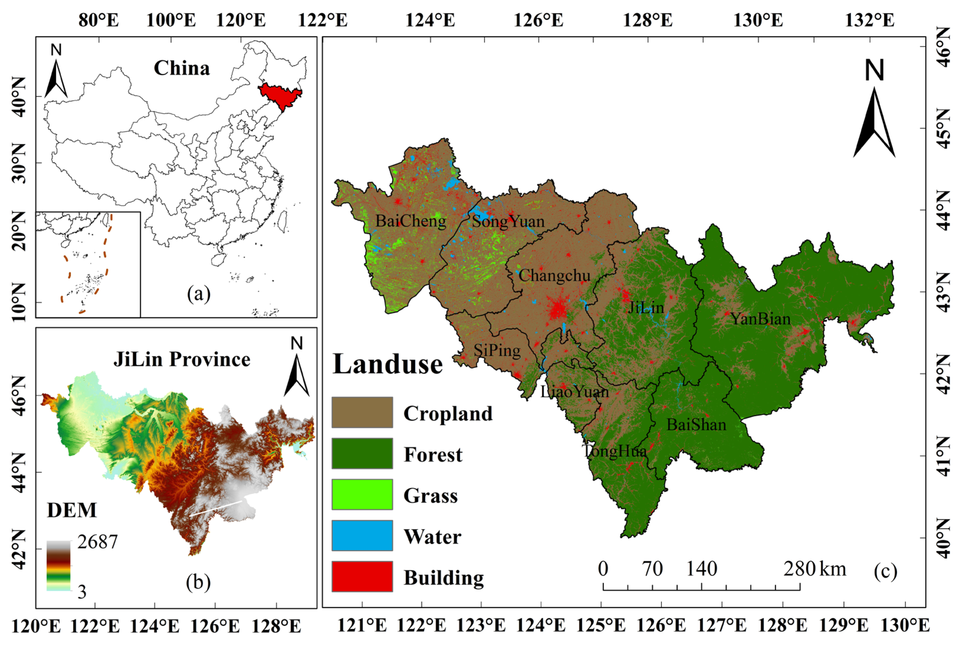
Jilin Province (40°52′–46°18′ N, 121°38′–131°19′ E), centrally located in northeastern China, is a key commercial grain base and ecological barrier, as well as a climate-sensitive zone, covering a total area of 1.87 × 10⁵ km² (Figure 1a). The landforms of Jilin Province consist of three major geographic units with distinct spatial heterogeneity in land-use patterns due to differences in topography, climate, and human activities [35,36]: the eastern mountainous areas dominated by the Changbai Mountain Range, featuring forested ecosystems and low-intensity agriculture; the central tableland plains, which serve as the core agricultural belt with cropland resources ranking fifth nationwide [37]; and the western alluvial plains facing acute ecological issues, where 12.3% of the area suffers from soil salinization, grass degradation, and desertification driven by a semi-arid climate and farming activities [38] (Figure 2).

Since 2000, policy-driven ecological restoration (e.g., farmland conversion to forest/grass), urban expansion, and climate shifts have collectively shaped land-use change in this region, forming a “mountain–plain gradient” where land-use intensity declines from the densely populated central plain to the ecologically fragile west [39]. These changes not only lead to prominent risks such as grain production capacity decline, ecosystem degradation, and benefit-distribution conflicts caused by cropland non-agriculturalization [11], but they also drive passive adaptive adjustments in land-use structure via climate warming-induced factors, further exacerbating the instability of cropland distribution and utilization patterns [40] and triggering ecological risks including black soil degradation and biological habitat fragmentation.

The spatiotemporal complexity of cropland changes in Jilin Province, coupled with the unclear key driving factors of cropland conversion under complex human–land interactions as well as ambiguous dynamic evolutionary pathways and multiscale effects, makes it an ideal case for exploring cropland change cascade pathways and their driving factors. Therefore, this study takes Jilin Province as the research area to explore the cascade pathways of cropland change and their driving factors using PLS–SEM, which is vital for addressing the critical issue of balancing cropland protection and development needs, breaking through the cognitive blind zone of the “cause–path–effect” chain in cropland change and safeguarding regional food security and coordinated, sustainable human–land development.

2.2. Data Sources and Processing

This study employed land-use, socioeconomic, topographic, soil, and meteorological datasets from 2010 to 2019, all resampled to a 30 m resolution (

Table 1. Data source and factor descriptions.

Data and Factors	Label	Sources (URL)	Data Product	Sensor/Platform	Resolution
Land-use data	——	https://zenodo.org/records/5816591 (accessed on 5 July 2025)	N/A	N/A	~30 m
Population quantity	PQ	https://zenodo.org/records/11179644 (accessed on 5 July 2025)	GPWv4.11	Census, satellite night-time lights, etc.	~1 km
Population density	PD	https://zenodo.org/records/11179644 (accessed on 5 July 2025)	Same as above	Same as above	~1 km
Gross domestic product	GDP	https://zenodo.org/records/13943886 (accessed on 5 July 2025)	N/A	N/A	0.08°
Greenhouse gas	GHG	https://edgar.jrc.ec.europa.eu/dataset_ghg80 (accessed on 5 July 2025)	EDGAR v8.0	Multiple (inventories, observation fusions)	0.1°
Temperature	Tem	https://data.tpdc.ac.cn/zh-hans/data/71ab4677-b66c-4fd1-a004-b2a541c4d5bf (accessed on 5 July 2025)	China1km	Meteorological station interpolation	1 km
Evapotranspiration	ET	https://lpdaac.usgs.gov/products/mod16a2gfv061/ (accessed on 5 July 2025)	MOD16A2GF V061-1	MODIS/Terra-1	500 m
Relative humidity	RH	https://data.tpdc.ac.cn/zh-hans/data/6854ebb3-8a60-454a-8d43-4e6a8c0ebd5d (accessed on 5 July 2025)	China1km	Meteorological station interpolation	1 km
Precipitation	Pre	https://data.tpdc.ac.cn/en/data/e5c335d9-cbb9-48a6-ba35-d67dd614bb8c (accessed on 5 July 2025)	China1km	Meteorological station interpolation	1 km
Digital elevation model	DEM	https://dwtkns.com/srtm30m/ (accessed on 5 July 2025)	SRTM V3 (SRTM30)-2-7	Space Shuttle Radar (C/X-band SAR)-7	~30 m
Slope	Slope
Land surface temperature	LST	https://www.resdc.cn/DOI/doi.aspx?DOIid=98&WebShieldSessionVerify=2453LOxMPjH8CkYOUcTA (accessed on 5 July 2025)	MYD11C3 (V6.1)	MODIS/Aqua	0.05°
Normalized difference vegetation index	NDVI	http://www.gis5g.com/data/zbsj/NDVI?id=24 (accessed on 5 July 2025)	MOD13A3 (V6.1)	MODIS/Terra	1 km
Leaf area index	LAI	http://www.geodoi.ac.cn/WebCn/doi.aspx?Id=3403 (accessed on 5 July 2025)	MOD15A2H (V6.1)	MODIS/Terra	500 m

). As croplands are directly affected by changes in the areas of other land categories, we analyzed the conversion relationships among different land types using land-use data. To systematically explore the drivers of spatiotemporal changes in croplands, we categorized the influencing factors into three broad categories, human activities, climate conditions, and geographic conditions, with the specific components of each category clearly defined as follows:

(1) Human activities factors: To capture the impact of human activities on spatiotemporal changes in croplands, we selected population quantity (PQ), population density (PD), and gross domestic product (GDP) as representative factors. These indicators can effectively reflect the intensity of human production and living activities, which are closely related to cropland occupation, reclamation, and management.

(2) Climate conditions factors: Climate is a key determinant of cropland change. Thus, the climate conditions category included greenhouse gases (GHGs), temperature (Tem), evapotranspiration (ET; reflecting the integrated impact of climatic factors), relative humidity (RH), and precipitation (Pre). These variables comprehensively characterize the climatic environment of the study area, which directly affects the suitability and productivity of croplands.

(3) Geographic conditions factors: Elevation, slope, and other geographical factors significantly influenced cropland changes. Considering the combined effects of surface soil, lithology, elevation, and topographic relief on LST heterogeneity, we included the digital elevation model (DEM, for extracting elevation), slope, and LST in the geographic conditions category to quantify the influences of geographical factors on croplands. Slope data were extracted from the DEM using ArcGIS 10.8.

Croplands were defined as the sum of cropland and wasteland areas. These datasets, encompassing the three aforementioned driver categories, adequately characterize natural environments and human activities. Furthermore, following established methodologies [41,42], 1 × 1 km grid cells were generated, with values extracted at grid points to support analyses including the optimal parameter geographic detector and PLS–SEM. Note that all observed variables in this study (i.e., the 14 indicators in Table 1) represent magnitude changes during 2010–2019. Datasets for Figure 3, Figure 4, Figure 5, Figure 6 and Figure 7 were also derived from this identical time span.

2.3. Technical Approach

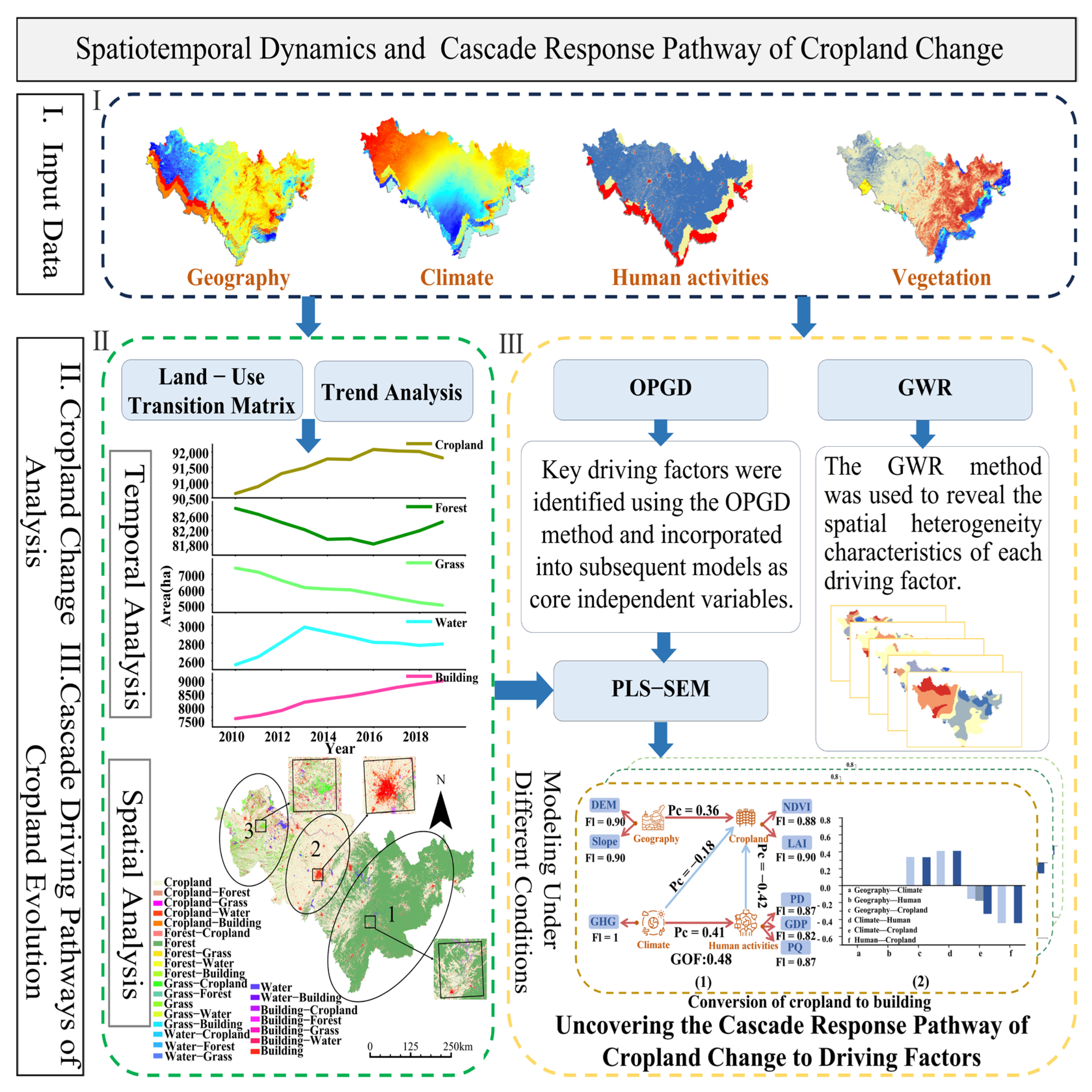
The technical framework of this study is illustrated in Figure 2, comprising three components: data input, cropland change analysis, and cascade driving pathways of cropland evolution. Details of the data input are provided in Section 2.1. For cropland change analysis, spatiotemporal conversion patterns and evolutionary trends of all land categories were quantified using 30 m resolution land-use data from 2010 to 2019, thereby elucidating the evolutionary trajectory of cropland change in Jilin Province. The cascade driving pathways of cropland evolution, constituting the core of this study, were analyzed through an integrated “OPGD-SEM-GWR” framework. First, the optimal parameters-based geographical detector (OPGD) in the GD package of RStudio 2024.09.1 was employed to automatically classify 13 natural and anthropogenic factors into 5–9 categories via five classification methods, and their Q-statistics (explanatory power) for cropland area were calculated. Second, the 13 observed variables were aggregated into four latent variables—geography (DEM, slope, LST), climate (GHG, Tem, ET, RH, Pre), human activities (PD, PQ, GDP), and cropland attributes (cropland area, NDVI, LAI)—to construct an initial structural equation model; significant factors corresponding to each latent variable were then screened based on the Q-values from the OPGD to develop an optimized PLS-SEM model. Finally, geographically weighted regression (GWR) was applied to estimate local regression coefficients between each factor and cropland area, quantifying their spatial driving intensities and revealing the heterogeneous impacts of these factors on cropland change. The detailed methodological principles are discussed in the following sections.

2.4. Land-Use Transition Matrix

The land-use transition matrix is a two-dimensional analytical tool used to quantify land-use states and dynamic relationships across temporal scales within a defined spatial domain. By counting the conversion areas between land-use types (e.g., cropland, forest, grass, and urban land) at two time points, this matrix systematically reveals bidirectional conversion pathways [42]. Its mathematical expression is:

$$\left|M\right|=\left[\begin{array}{cccc}{A}_{11}& A_{12}& \dots & A_{1n}\\ A_{21}& A_{22}& \dots & A_{2n}\\ ⋮& ⋮& \ddots & ⋮\\ A_{n1}& A_{n2}& \dots & A_{nn}\end{array}\right]$$

(1)

where $A_{ij}$ represents the area converted from land-use types I to j, and n is the total number of categories. Diagonal elements ($A_{ii}$) reflect stable unchanged areas, while off-diagonal elements ($A_{ij}, i\ne j$) characterize the scale and direction of conversion between types.

2.5. Optimal Parameters-Based Geographical Detector

Geographic detection is a novel statistical method for detecting spatial heterogeneity and identifying the driving factors. It makes no linear assumptions, features a parsimonious mathematical form, and offers clear physical interpretability. The core premise is that if an independent variable influences a dependent variable, their spatial distributions should be similar. The method works by analyzing within-layer and between-layer variances to calculate the single-factor q-value and multi-factor superimposed q-value, determining whether interaction effects or other relationships exist between factors [43]. The formula is:

$$q=1-{\displaystyle \frac{1}{N{\sigma }^2}}{\displaystyle \sum _{n=1}^L{N}_h}{\sigma }_h^2$$

(2)

where $q$ is the spatial heterogeneity of an indicator, $N$ is the total number of samples in the study area, ${\mathsf{\sigma }}^2$ is the variance of the indicator, $h$ denotes the partition, and $L$ is the number of partitions for the independent or dependent variable. The value of $q$ ranges from [0 to 1], and a larger value indicates stronger spatial heterogeneity.

The optimal parameter geographic detector, which is an extension of the geographic detector, identifies the ideal classification parameters by comparing the q-values from different discretization methods and breakpoint numbers. The choice of discretization method and breakpoint count is critical for maximizing the q-value, which measures the explanatory power of independent variables for dependent variables [44,45,46]. Five discretization methods were used: standard deviation (SD), natural breaks (NB), equal interval (EI), quantile (QC), and geometric interval (GI). Existing studies show that too many or too few breakpoints cause information redundancy or loss; therefore, we set breakpoint numbers between five and nine. The driving factors for each land-use type were identified using the factor and interaction detector results.

2.6. Partial Least Squares Structural Equation Modeling

PLS–SEM is a multivariate technique that reveals complex causal relationships by connecting latent variables (unobservable constructs) to manifest variables (directly measurable indicators). Unlike covariance-based SEM, PLS–SEM—grounded in principal component analysis—is better suited for small samples, non-normal data, and formative and reflective measurement models [29,47]. PLS–SEM prioritizes the variance explanation over model fit, making it highly suitable for exploratory research and predictive analysis. Its ability to handle formative constructs (e.g., indices composed of multiple indicators) and mitigate multicollinearity make it ideal for analyzing multidimensional land-use drivers [e.g., socioeconomic policies and ecological constraints] [47]. The formula is:

$$X={\mathsf{\Lambda }}_x\xi +\delta$$

(3)

$$Y={\mathsf{\Lambda }}_y\eta +\epsilon$$

(4)

where $X$ and $Y$ are vectors of exogenous and endogenous indicators, respectively; $\xi$ and $\eta$ are vectors of exogenous and endogenous latent variables, respectively; ${\mathsf{\Lambda }}_{\mathrm{x}}$ and ${\mathsf{\Lambda }}_{\mathrm{y}}$ are parameter matrices to be estimated; and $\delta$ and $\epsilon$ are measurement error terms.

$$\eta =B\eta +\mathsf{\Gamma }\xi +\zeta$$

(5)

where ${\rm B}$ is the matrix of path coefficients among endogenous latent variables, $\mathsf{\Gamma }$ is the matrix of path coefficients from exogenous to endogenous latent variables, and $\zeta$ is the structural error term.

Goodness-of-fit (GOF) is a core metric for evaluating the overall validity of PLS-SEM. It is defined as the geometric mean of the average communality of all latent variables and the average coefficient of determination (R²) of the endogenous latent variables [48]. The formula is:

$$\mathrm{GOF}=\sqrt{\overline{\mathrm{communality}}\times \overline{R^2}}$$

(6)

This metric provides a practical solution for testing the global validity of PLS models, serving a dual purpose for both the measurement model and the structural model: on the one hand, communality reflects the extent to which latent variables explain their observed indicators, characterizing the intrinsic quality of the measurement model; on the other hand, R² measures the explanatory power of exogenous latent variables for endogenous latent variables, reflecting the predictive power of the structural model. By integrating these two aspects, GOF offers a comprehensive measure of the overall fit of a PLS model, enabling researchers to simultaneously assess the explanatory power of the measurement model and the structural model within a unified framework, thereby providing a concise and effective basis for judging the model’s global suitability.

In this study, geographic factors, climatic factors, human activities, and three land-use types (cropland, forest, and grass) were defined as latent variables, with separate PLS–SEM models constructed for each category. We used 13 observed variables to quantify the impact of external factors on cropland transitions and analyze the interactive relationships among land-use types. This framework allows for the simultaneous estimation of measurement and structural relationships, illuminating how latent constructs (e.g., socioeconomic drivers and ecological constraints) influence cropland changes.

2.7. Geographically Weighted Regression

The core advantage of GWR is its ability to capture non-stationary relationships and scale dependency between explanatory and response variables by integrating geographic spatial parameters. This method incorporates spatial weighting functions into a traditional regression and quantifies spatial heterogeneity through spatially explicit variable relationships [39,41,42,44]. Compared with traditional global regression models, GWR not only reveals spatial differentiation patterns of land-use change drivers but also accurately characterizes variations in driver influence intensity across geographic units. This feature gives it unique value in spatial analysis by addressing the limitations of PLS–SEM in capturing driver spatial heterogeneity. The formula is:

$$y_i={\beta }_0(u_i,v_i)+{\displaystyle \sum _{k=1}^m{\beta }_k}(u_i,v_i)x_{ik}+{\epsilon }_i$$

(7)

where ${\mathrm{y}}_{\mathrm{i}}$ represents the value of the dependent variable at location $\mathrm{i}$, ${\mathrm{x}}_{\mathrm{i}\mathrm{k}} (\mathrm{k}=\mathrm{1,2},\cdots \mathrm{m})$ denotes the value of independent variable k at location $\mathrm{i}$, $\left({\mathrm{u}}_{\mathrm{i}},{\mathrm{v}}_{\mathrm{i}}\right)$ are the coordinates of regression point $\mathrm{i}$, ${\mathsf{\beta }}_0\left({\mathrm{u}}_{\mathrm{i}},{\mathrm{v}}_{\mathrm{i}}\right)$ is the intercept term, and ${\mathsf{\beta }}_{\mathrm{k}}\left({\mathrm{u}}_{\mathrm{i}},{\mathrm{v}}_{\mathrm{i}}\right)\left(\mathrm{k}=\mathrm{1,2},\cdots \mathrm{m}\right)$ are the regression coefficients.

3. Results

3.1. Spatiotemporal Evolution of Land Use in Jilin Province

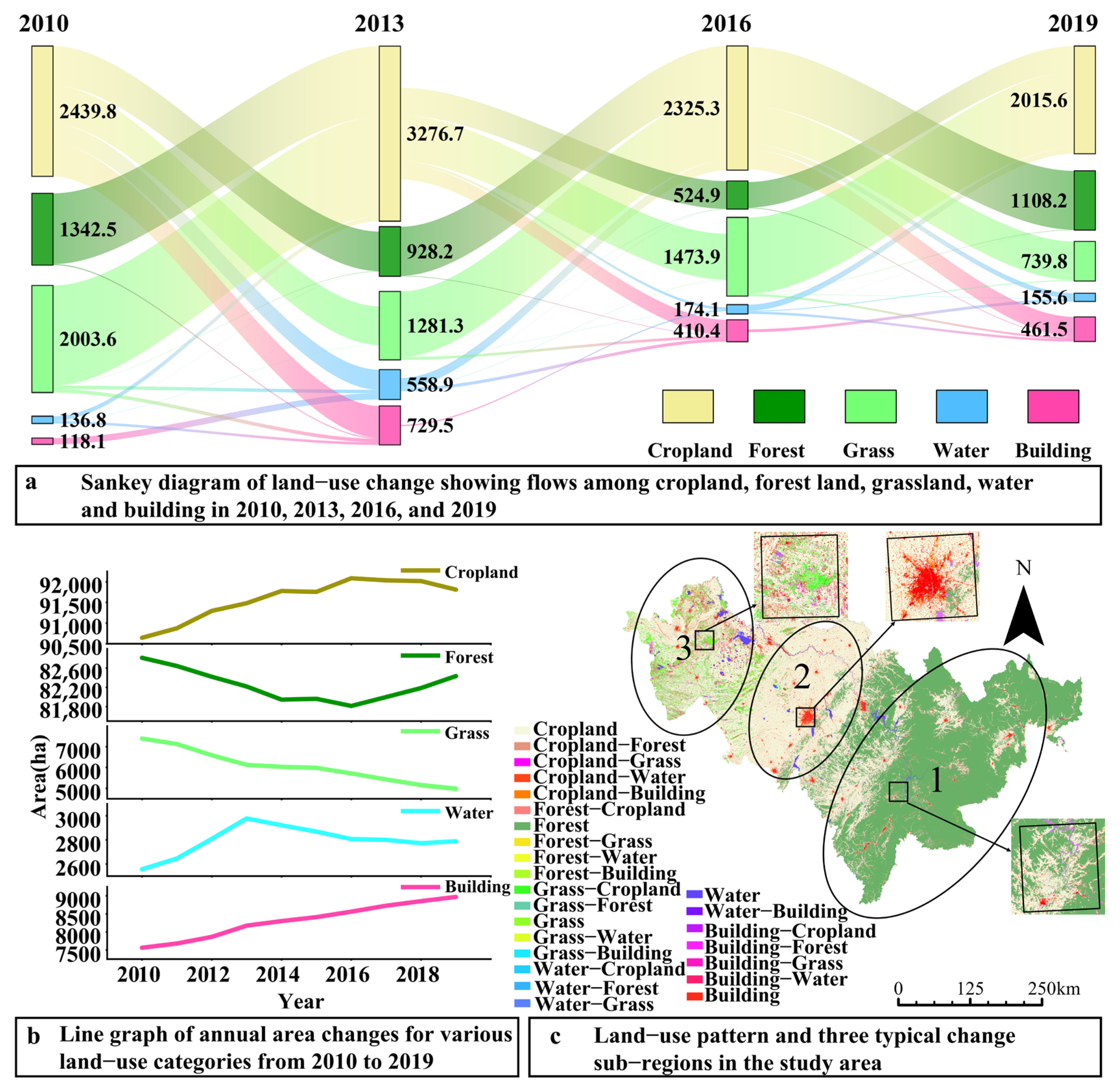
The area changes of different land types from 2010 to 2019 are ranked in descending order of their absolute values, as follows: grassland (decrease of 2425.7 ha), built-up land (increase of 1406.2 ha), cropland (increase of 1165.3 ha), forest land (decrease of 378.5 ha), and water area (increase of 232.8 ha). These changes correspond to 32.77%, 15.68%, 1.27%, 0.46%, and 8.35% of the respective land areas in 2010. Changes in land area by land type from 2010 to 2019, ranked in descending order based on their proportion of total land area in 2010, are as follows: grassland decreased by 32.77% (2425.7 ha), construction land increased by 15.68% (1406.2 ha), water bodies increased by 8.35% (232.8 ha), cultivated land increased by 1.27% (1165.3 ha), and forested land decreased by 0.46% (378.5 ha). Cropland net conversion to other land types occurred in three consecutive 3-year periods (2010–2013, 2013–2016, 2016–2019) at the rates of 2.69% (2439.8 ha), 1.88% (1721.9 ha), and 2.40% (2209.6 ha), respectively, with a total of 6452 ha of cropland converted out—among which 1257.7 ha was converted to built-up land. In contrast, the conversion of other land types to cropland in the same three periods was recorded at 3.58% (3276.7 ha), 2.53% (2325.3 ha), and 2.20% (2015.6 ha), respectively (Figure 3a), with the total cropland gain dominated by forestland (2720.2 ha) and grassland (4518.8 ha) conversion. Over the entire decade, built-up land underwent a cumulative expansion of 18.59% (1406.2 ha), which was primarily realized at the cost of cropland. Water bodies showed a negligible net change in area but experienced frequent mutual conversions with cropland and built-up land, which indicates that surface water dynamics were dominated by human activities (Figure 3a).

The temporal dynamics of each land category are presented in Figure 3b. Cropland area increased gradually from 90,644.4 ha in 2010 to a peak of 92,084.8 ha in 2016 (a 1.59% rise), then declined to 91,809.7 ha in 2019 (equivalent to a 1.29% increase relative to 2010). Forestland exhibited a steady annual decrease, reaching a minimum of 81,814.6 ha in 2016 (a 1.20% reduction from 2010), followed by a subsequent recovery. Grassland area decreased continuously, with a 32.77% reduction (2425.7 ha) in 2019 compared to 2010 levels. Water bodies showed an overall increasing trend, peaking at 2978.1 ha in 2013 (a 9.11% increase relative to 2010), which was likely linked to heavy rainfall in Jilin Province that year (https://news.sina.com.cn/c/2013-08-16/225427970707.shtml, accessed on 5 July 2025). Built-up land area increased annually from 7564.3 ha in 2010 to 8970.4 ha in 2019, representing an 18.59% cumulative increase. Cropland area dynamics reflected inter-category land competition, rising initially to a peak of 92,084.8 ha (a 1.59% increase relative to 2010) in 2016 before undergoing a steady decline thereafter. Notably, the cropland and forest area change curves show a mirror-like pattern (Figure 3b), which is likely linked to policies such as cropland-to-forest conversion.

Spatially, the eastern region of Jilin Province was dominated by forest–cropland conversions (Figure 3c-1), while the central region showed cropland-to-building transitions (Figure 3c-2) driven by urban expansion. In the west, grass and cropland were frequently converted into each other (Figure 3c-3), mainly because of grass reclamation under the land reclamation balance policy. The spatial patterns of land-use change exhibited fragmented multimodal distributions with pronounced heterogeneity (Figure 3c). Overall, dominant land-use conversions in the study area were “cropland to construction land,” “forest to cropland,” and “grass to cropland.”

3.2. Key Driving Factors of Cropland Change

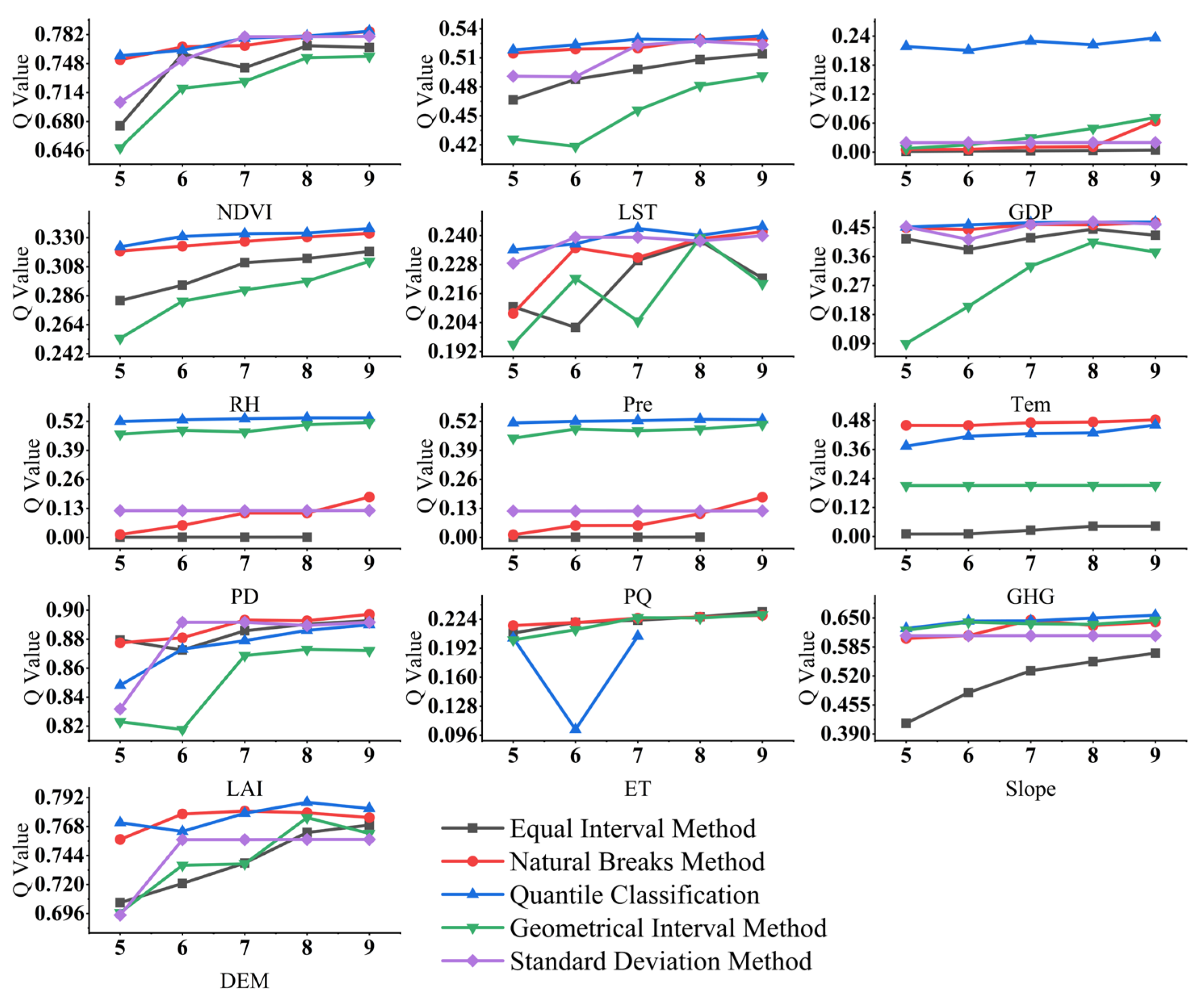
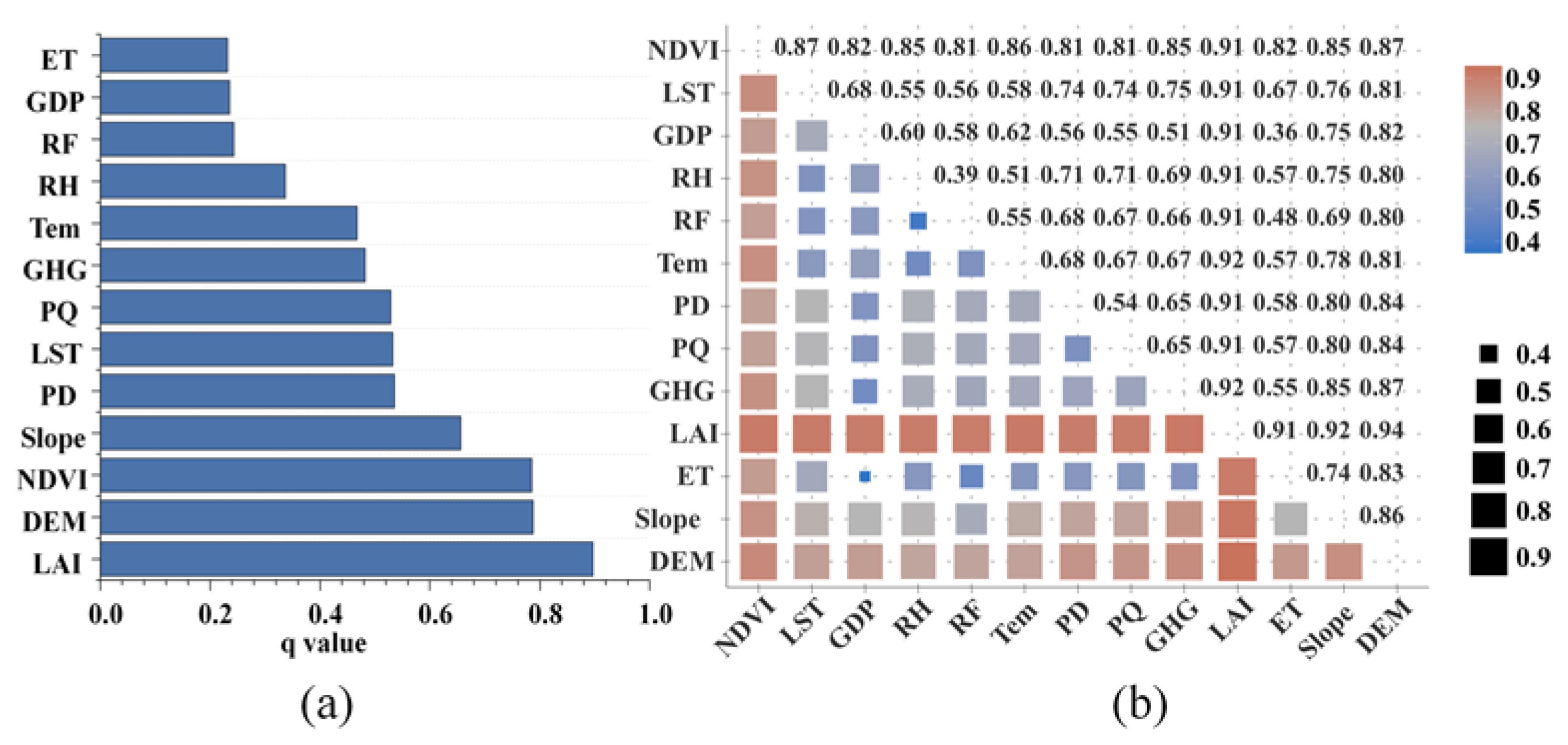
Beyond land category conversions (Figure 3), cropland dynamics are influenced by complex environmental variables [49]. To systematically quantify the explanatory power of these drivers, we adopted the optimal parameters-based geographical detector (OPGD) model. The results reveal notable differences in optimal classification schemes across variables. NDVI, LST, GDP, RH, Pre, GHG, and slope achieved relatively higher Q-values (0.79, 0.53, 0.24, 0.34, 0.24, 0.48, and 0.66, respectively) when classified into nine classes using quantile classification. In contrast, PD, PQ, and DEM achieved relatively higher Q-values (0.54, 0.53, and 0.79, respectively) when categorized into eight classes using the same quantile approach. LAI and ET reached maximum Q-values of 0.90 and 0.23 via nine-class NB classification, while Tem obtained an optimal Q-value of 0.47 through eight-class SD classification. This indicates that, in addition to vegetation indices (LAI and NDVI), geographic factors (DEM, slope) appear to strongly influence land cover types. Among the human activity indicators, population density (PD) showed relatively strong explanatory power (Q > 0.5), while climate factors generally exhibited weaker effects. GHG had a relatively stronger influence (Q = 0.48), and ET had the smallest influence (Q = 0.23).

The interaction detector evaluates the interactive effects of the driving factors on land category changes. The interactive explanatory power of LAI with other driving factors was significantly removed, only left enhanced, with all Q-values exceeding 0.91 (Figure 5b). The interactive explanatory power of ET and GDP was relatively low (Q = 0.36) but still showed enhanced effects compared with their individual Q-values (ET = 0.23, GDP = 0.24). These results suggest that the driving factors may not only exhibit individual explanatory advantages but also jointly influence cropland changes through interactions with other factors. Therefore, revealing their direct and indirect effects on cropland changes remains necessary, though such inferences should be supported by complementary analytical approaches.

3.3. Cascade Pathways of Driving Factors and Cropland

3.3.1. Accuracy of Partial Least Squares Structural Equation Modeling

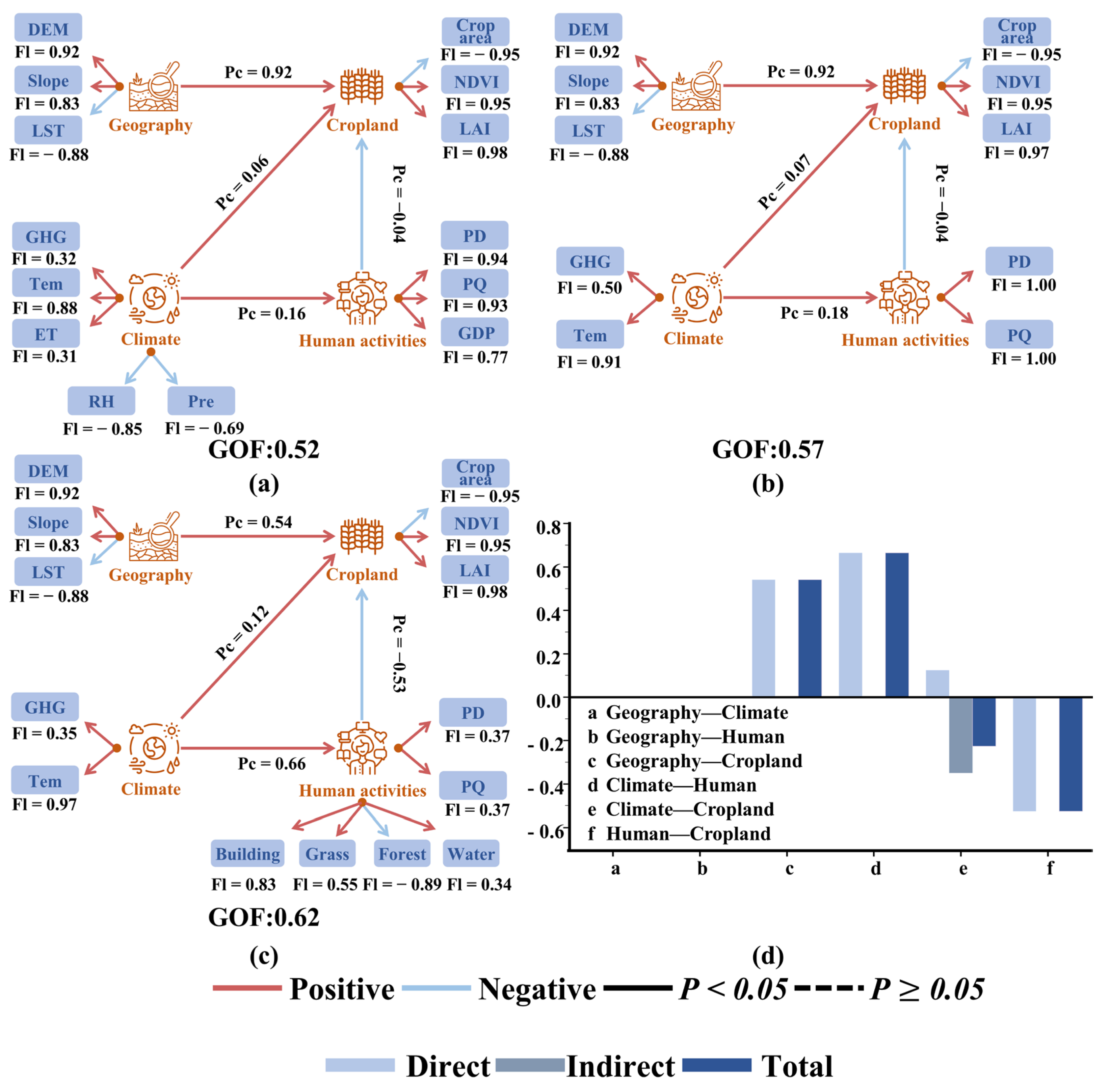
Based on OPGD screening based on Q-values to exclude weakly explanatory variables (ET, RH, Pre and GDP) and incorporating land-use conversion variables, we constructed a partial least squares structural equation model (PLS–SEM) encompassing four latent variables—geography, climate, human activities and croplands—to uncover the driving mechanisms of cropland change. The GOF index assesses the overall fit of the PLS–PM model, with values ranging from 0 to 1 (higher values indicate a better fit). As shown in Figure 6, removing invalid observed variables via the OPGD method increased the GOF from 0.52 to 0.57, and all path coefficients improved (Figure 6a,b). Adding land-use area as an observed variable for the human activity latent variable further enhanced both the GOF value and path coefficients (Figure 6c). These results demonstrate that the proposed PLS–SEM modeling approach significantly improves model performance.

3.3.2. Cascading Path Analysis of Cropland and Driving Factors

In the PLS–SEM model, the path coefficient (Pc) between the latent variables measures direct influence. The product of the Pc values along a path quantifies the indirect effect of the initial latent variable on the final latent variable. A positive Pc indicates that a unit change in the predictor variable yields a change in the Pc magnitude in the response variable.

The revised PLS–SEM model identified geography and human activities as the primary drivers of cropland distribution changes, with climate having a weaker impact (Figure 6c,d). The direct path coefficients for the three factors were 0.5405, −0.5271, and 0.1235, indicating the positive effects of geography and climate on croplands, whereas human activities exerted a negative influence. Key findings include the following: (1) Areas with higher DEM and slope (and lower LST; that is, mountainous regions) show smaller cropland areas, confirming cropland shrinkage in unsuitable mountainous areas and expansion in high-yield plains regions. This aligns with the low-altitude grassland-to-cropland conversion shown in Figure 3c-3 (consistent with the spatial pattern in Figure 2II). (2) Increases in PD and PQ drive cropland expansion and vegetation decline, as evidenced by the high factor loadings for the NDVI (0.9471) and LAI (0.9753). (3) Forest expansion emerged as a key land-use factor that reduces croplands, reflecting the impact of human-driven policies such as farmland-to-forest/grass conversion. (4) Regional increases in GHGs and Tem promote vegetation growth but also contribute to cropland reduction. Notably, climate elements strongly influenced human activities (path coefficient = 0.664), with the indirect climate effect on cropland via human activities measuring −0.3500. The total effect (direct + indirect) was −0.2266 (Figure 6d), highlighting the indirect negative risks of climate change to agricultural security, which warrant urgent attention.

3.3.3. Cascade Paths of Change for Cropland, Forest, and Grass in Three Typical Land-Use Conversion Regions

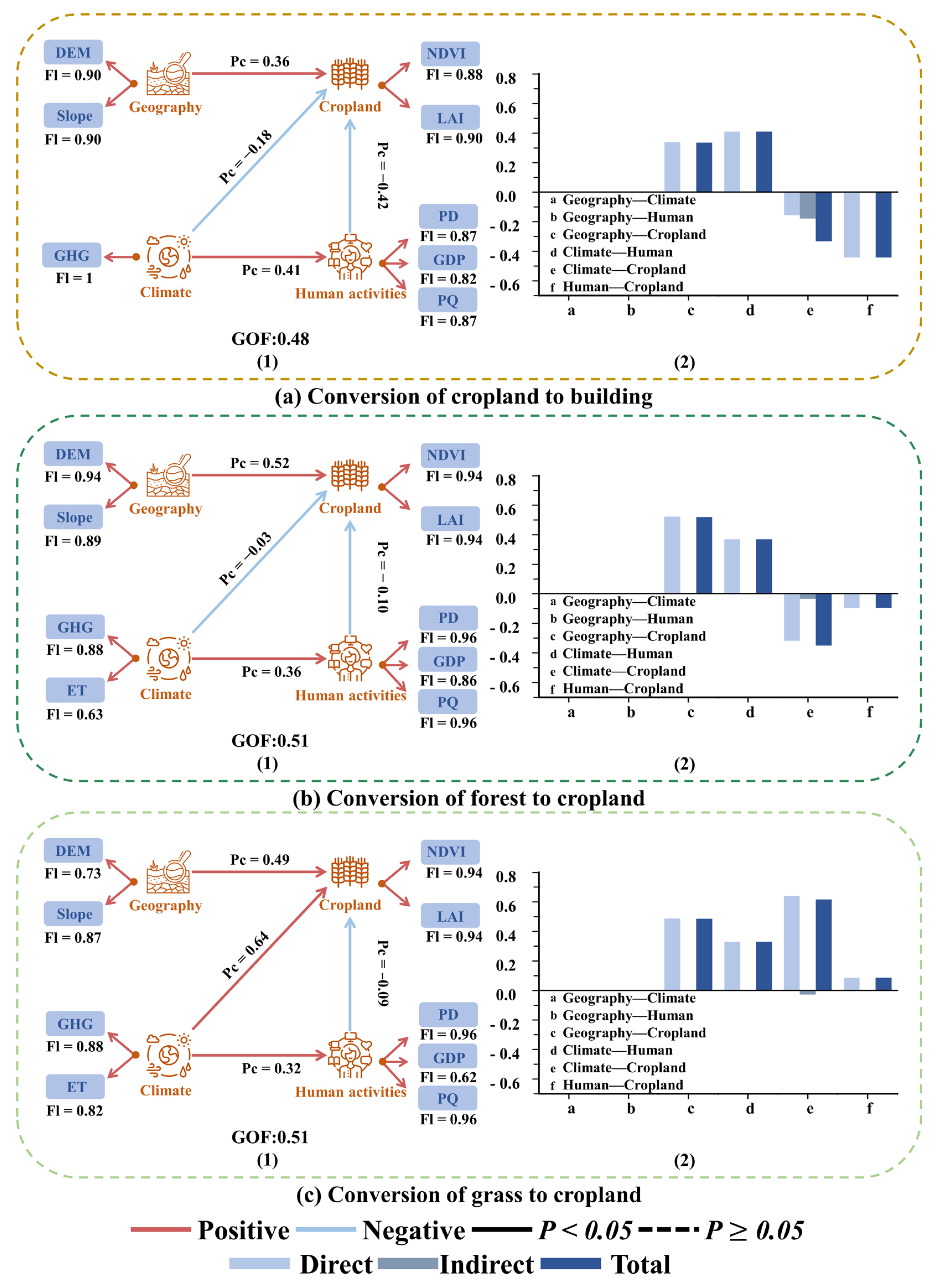
Figure 6 illustrates the cascading path response of cropland changes to the influencing factors at a regional scale. To explore the cropland’s change mechanisms at the microscale, we selected three typical conversion types, cropland-to-building, forest-to-cropland, and grassland-to-cropland (Figure 3c(1–3)), and developed separate PLS–SEM models for each (Figure 7).

In a typical cropland-to-construction area (Figure 3c-2), DEM and slope were key geographic factors, whereas LST lost its driving role. GHG emerged as the primary climatic factor, with PD, PQ, and GDP being the dominant drivers of human activity (Figure 7a-1). The direct effects of geography, human activities, and climate on croplands were 0.3605, −0.4214, and −0.1759, respectively (Figure 7a-1). Compared with the regional scale (Figure 6c), the effect of climate on croplands shifted from positive to negative, although only marginally, with its indirect effect remaining negative. This yields a total climate effect of −0.3496 on cropland, combining direct (−0.1759) and indirect (−0.1737) impacts (Figure 7a-2). In the forest-to-cropland area (Figure 3c-1), croplands are dominated by geographic factors, with diminishing human activity and climate impacts, likely owing to the high topographic relief in mountainous regions (Figure 7b). Conversely, the grassland-to-cropland area (Figure 3c-3) showed exclusive climatic factor dominance, an unprecedented pattern absent at the regional scale or in other conversion types, highlighting the need to prioritize climate change risks in regional agricultural production. The detailed path coefficients (direct/indirect) and factor loadings of the latent variables are shown in Figure 7.

3.4. Impact of Manifest Variable Spatial Heterogeneity on Cropland

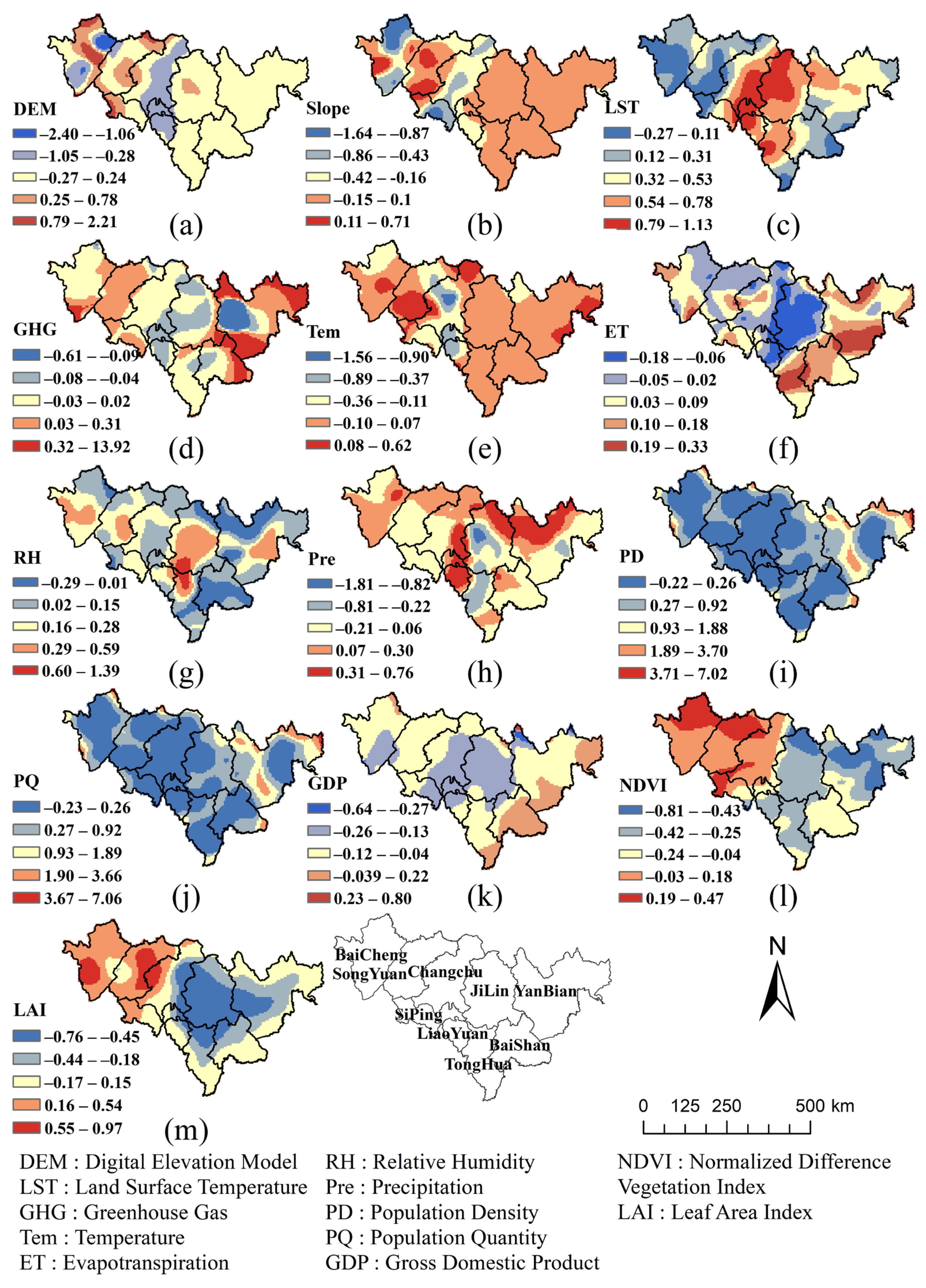
The GWR outputs reveal pronounced spatial nonstationarity in how these factors shape cropland dynamics. The 13 factors can be separated into three distinct categories based on overall heterogeneity. The first category—DEM, slope, and Tem—showed concentrated heterogeneity in the central–western region (Figure 8a,b,e), with regression coefficients ranging from −2.398 to 2.208, −1.638 to 0.707, and −1.563 to 0.619, respectively. These act as key drivers of cropland change in the central–western areas. The second category—Pre, PD, PQ, GDP, and NDVI—exhibited heterogeneity mainly in the central–eastern region (Figure 8h–l), with lower spatial variability in the west, indicating their dominant role in driving cropland change in eastern mountainous areas. The third category comprises factors with strong spatial heterogeneity across the entire region (Figure 8c,d,f,g,m), exerting significant driving forces on cropland change at the regional scale.

In terms of impact polarity and magnitude, DEM, slope, and Tem predominantly exhibit negative effects on cropland area, with only isolated small regions showing regression coefficients > 0.1 (positive values). Among the second-category factors, Pre generally exerted a positive impact on cropland expansion across large areas (regression coefficients: −1.81 to 0.76), whereas the remaining factors (PD, PQ, and GDP) showed negative effects for >90% of the study area. Specifically, PD and PQ exhibited remarkably similar spatial heterogeneity patterns with similar regression coefficients. Except for a small northeastern area that showed a positive correlation, both factors predominantly demonstrated a negative correlation. GDP regression coefficients range from −0.64 to 0.80, with negative correlation areas mainly concentrated in the Changchun and Jilin regions. Additionally, NDVI and LAI (third-category factors) showed negative correlations with cropland area changes in eastern Jilin Province, but they displayed distinct spatial heterogeneity and strong positive correlations in central and western regions. Their regression coefficients ranged from −0.81 to 0.47 and −0.76 to 0.97, respectively. In the third factor category, LST showed a positive correlation centered on Changchun, decaying outward, with regression coefficients ranging from −0.27 to 1.13. GHG exhibited regression coefficients of −0.61 to 13.92, with a strong positive correlation, which was notably observed in the Yanbian region. The ET regression coefficients ranged from −0.18 to 0.33, transitioning from negative to positive correlation from the center outward. RH had regression coefficients of −0.29 to 1.39.

The spatial distribution patterns of the impacts of these 13 factors on croplands provide deeper insights into the driving mechanisms of cropland area changes, offering theoretical and data-driven support for subsequent land-use planning.

4. Discussion

4.1. Driving Pathways for Cropland Conversion

This study quantified the spatiotemporal cropland conversions across western, central and eastern Jilin Province and further decoupled the direct and indirect cascade driving paths of terrain, climate and human socioeconomic factors based on a multi-model coupling framework. Our results revealed that around 6452 ha of cropland was transformed into built-up land during 2010–2019, and human activity represented the dominant driver behind cropland non-agricultural occupation in central plains, with a path coefficient of −0.527 at provincial scale and −0.421 in central urban expansion zone, which was consistent with previous research on rapid urban sprawl in Northeast China’s core grain-producing plains [39,50]. Driven by GDP growth and population agglomeration around Changchun and Jilin urban agglomeration, continuous construction land expansion directly eroded high-quality flat cropland, which is a common land-use conflict in China’s major agricultural zones [10].

Nevertheless, human socioeconomic factors exerted limited impacts on forest-to-cropland and grassland-to-cropland regions in eastern mountains and western plains. Such spatial discrepancy originates from differentiated land management policies: eastern forest reclamation is restricted by natural forest protection projects, while western grass reclamation is largely regulated by cropland requisition–compensation balance policy [38]. Topographic factors showed consistently positive direct effects on cropland distribution across all three subregions, with path coefficients ranging from 0.361 to 0.541. Plains areas with low elevation and gentle slope have superior hydrothermal conditions for agricultural cultivation, thus becoming priority regions for cropland expansion either from forest clearance or grassland reclamation [51].

Consistent with the core research objective of climate-mediated cascade effects, climatic factors rarely alter cropland area directly at the provincial level but dominantly regulate land-use variation indirectly via modifying human production and cultivation behaviors (Climate → Human path coefficient = 0.664). This human-mediated cascade path explains why rising greenhouse gas concentration and temperature do not directly shrink or expand cropland on the whole, but they change farmers’ willingness for wasteland reclamation and intensive farming modes. Distinctively, climate switched into a direct dominant driver in western semi-arid grassland areas (direct path coefficient = 0.637). The western plain is ecologically fragile with severe salinization and water shortage; precipitation, temperature and humidity fluctuations directly determine grassland survival status, and favorable climatic conditions stimulate large-scale grassland-to-cropland reclamation without intermediate human socioeconomic interference [40]. The differentiated direct/indirect climate effect among subregions supplements existing research which generally ignored spatial divergence of climate–cropland interaction in Northeast China.

4.2. Analysis of Spatially Heterogeneous Drivers of Cropland Change

According to GWR spatial coefficient distribution, terrain indicators (DEM, slope), thermal condition (temperature), human indicators (PD, PQ, GDP) and vegetation indexes (NDVI, LAI) displayed obvious zonal heterogeneous effects on cropland dynamics across Jilin. Topography and temperature dominated cropland variation in central–western plains where flat terrain concentrates most high-yield cropland resources; small fluctuations in elevation and slope will greatly change agricultural suitability and further affect cropland layout [35]. In contrast, precipitation, population density and economic development dominated eastern mountain cropland changes because fragmented terrain restricts large-scale centralized construction, and cropland expansion mainly relies on scattered forest land development driven by local population growth and rural economic demand [36].

GHG, relative humidity and evapotranspiration showed province-wide universal impacts on cropland dynamics. Rising greenhouse gas improves regional accumulated temperature and extends the crop growing period, which promotes vegetation restoration and further restricts blind wasteland reclamation across the whole study area [8,16]. Spatially negative correlations between population, GDP and cropland in the Changchun–Jilin metropolitan area matches the universal law of urbanization-induced cultivated land loss across China’s metropolitan peripheries [18]. Meanwhile, the negative coefficient reversed to positive in remote western counties, which benefit from cropland balance policy that encourages developing unused saline–alkali and grassland into new cropland to offset urban cropland loss [38].

The cascade driving mechanism summarized in this study has wide reference value for mid-latitude monsoon agricultural regions globally. On the national scale, terrain constrains cropland spatial allocation by redistributing surface hydrothermal resources nationwide [51]. Globally, anthropogenic climate change modifies regional drought risk and crop productivity, further inducing passive cropland expansion or abandonment in South Asia and global grain belts [52,53]. The existing literature has verified the correlation between climate, human activity and cropland, but few studies systematically quantified multi-level indirect cascade pathways; our OPGD-PLS-SEM-GWR coupled framework makes up this research gap and can be transplanted to analogous agricultural regions worldwide for food security assessment.

4.3. Strengths and Limitations of This Research

4.3.1. Research Strengths

This study constructed an integrated “factor screening-pathway quantification-spatial heterogeneity characterization” framework coupling OPGD, PLS-SEM and GWR, effectively solving two core defects of single model application in traditional cropland research: the inability of geographic detectors to distinguish direct/indirect driving paths and the deficiency of global PLS-SEM in depicting spatial coefficient differentiation. The OPGD optimizes variable discretization parameters to calculate reliable q-values and filter invalid explanatory indicators, improving the rationality and fitting degree of the subsequent PLS-SEM model (GOF improved from 0.52 to 0.62 after variable optimization). Follow-up GWR supplements spatial information for latent variable path results and visually displays the regional differentiated influence of each manifest factor on cropland.

Methodologically, this study puts forward a mature variable preprocessing workflow for SEM land-use research, which can reduce artificial parameter bias in model construction and provide a referable analytical paradigm for subsequent LUCC driving mechanism research. Empirically, we distinguished three typical cropland conversion zones and separately built subregional PLS-SEM models, revealing the shift of climate from indirect mediator to direct driver in western grass–cropland transition areas, which enriches the cognition of regional climate–land interaction rules in the Northeast black soil region.

4.3.2. Research Limitations and Future Research Prospect

First, factor rankings based on Q-values are highly sensitive to discretization strategies and temporal aggregation approaches. The subtle differences in explanatory power among certain driving factors imply that the ranking of dominant factors may vary across alternative classification schemes and multi-temporal scales rather than reflecting a fixed contribution hierarchy. Consequently, the factor detection results in this study reflect the spatial explanatory power of each driver within the specified 1 km annual grid analysis framework and should not be generalized to other spatial or temporal scales. Future research can adopt machine learning-based automatic classification to improve the precision of factor detection. Second, this research only selects 13 natural and socioeconomic indicators, lacking explicit quantitative policy indicators such as implementation intensity of Grain-for-Green and cropland balance policies; although policy impacts are indirectly reflected via human activity variables, quantitative introduction of policy dummy variables can further perfect the cascade path logic.

Third, OPGD, PLS-SEM and GWR are all correlation-based statistical models; our results reveal statistical association pathways rather than strict causal relationships, consistent with the discussion in former research limitations. Incorporating the Granger causality test or causal discovery algorithm can help distinguish real causal links from spurious correlation in subsequent data processing [54]. Fourth, the fishnet grid extraction method used in variable matching may split natural administrative and terrain boundaries and bring minor sampling bias; vector zoning statistics based on county administrative units can optimize dataset construction in follow-up work.

In addition, this study only focuses on cropland area variation during 2010–2019 without involving cropland quality change (black soil degradation, soil fertility decline). Black soil quality is critical for regional food security; hence, future research can integrate soil organic matter and field survey data to explore cascade effects of climate and human activities on both cropland quantity and quality. Extending research time series to 2000–2025 is also helpful for identifying long-term climate change-driven cropland evolution trends.

5. Conclusions

Cropland conversions in Jilin from 2010 to 2019 displayed prominent zonal divergence: central cropland was encroached upon by built-up land, eastern forests were reclaimed for cropland, and western grasslands were turned into cultivated fields. In total, 7.12% (6452 ha) of cropland shifted to non-farm uses, including 1.39% (1258 ha) for construction; newly added cropland was derived from 3.01% (2720 ha) forest and 4.99% (4519 ha) grassland, controlled jointly by terrain, climate and regional socioeconomic gaps.

PLS-SEM quantified three critical cascading paths. Topography directly structured cropland distribution (Pc = 0.5405), while human activities induced central cropland loss (Pc = −0.5271). Region-wide climate impacts were mostly indirect via human regulation (Climate → Human: 0.664), yet climate directly dominated western grass-to-cropland conversion (Pc = 0.6367) under semi-arid conditions.

GWR revealed spatially heterogeneous drivers: terrain and thermal factors governed central–western cropland changes; precipitation, population, GDP and vegetation indices dominated eastern variations; and GHG, humidity and ET affected cropland across the whole province. Urban expansion around Changchun–Jilin caused severe cropland shrinkage, offset partially by the cropland requisition–compensation balance policy in western remote areas.

The integrated OPGD–PLS-SEM–GWR framework resolves the limitation of single models in separating direct and indirect cascading effects. These findings advance cropland driving mechanism theory and support targeted black soil and farmland protection for Northeast China and comparable global grain bases.

References

1. Zhang, X.; Hao, S.; Cui, Y.; Zhang, H. Study on the response of ecological sensitivity to land use and land cover changes in Jinzhai, China. Geocarto Int. 2024, 39, 2390491. [Google Scholar] [CrossRef]
2. Hinz, R.; Sulser, T.B.; Hüfner, R.; Mason-D’Croz, D.; Dunston, S.; Nautiyal, S.; Ringler, C.; Schüngel, J.; Tikhile, P.; Wimmer, F. Agricultural development and land use change in India: A scenario analysis of trade-offs between UN Sustainable Development Goals (SDGs). Earth’s Future 2020, 8, e2019EF001287. [Google Scholar] [CrossRef]
3. Kashyap, R.; Kuttippurath, J. Warming-induced soil moisture stress threatens food security in India. Environ. Sci. Pollut. Res. 2024, 31, 59202–59218. [Google Scholar] [CrossRef] [PubMed]
4. Li, Q.; Peng, X.; Frauenfeld, O.W.; Wu, Z.; Wang, Y.; Mu, C. Extreme rainfall reshapes permafrost thermal regimes across the Northern Hemisphere. Nat. Commun. 2026, 17, 3204. [Google Scholar] [CrossRef] [PubMed]
5. Hultgren, A.; Carleton, T.; Delgado, M.; Gergel, D.R.; Greenstone, M.; Houser, T.; Hsiang, S.; Jina, A.; Kopp, R.E.; Malevich, S.B. Impacts of climate change on global agriculture accounting for adaptation. Nature 2025, 642, 644–652. [Google Scholar] [CrossRef] [PubMed]
6. Kashyap, R.; Kuttippurath, J.; Patel, V.K. Agriculture intensification and moisture-induced Thar desert greening: Implications for energy balance, socio-economy, and biodiversity. GIScience Remote Sens. 2025, 62, 2483458. [Google Scholar] [CrossRef]
7. Yuan, J.; Chen, W.; Zeng, J. Spatio-temporal differentiation of cropland use change and its impact on cropland NPP in China. J. Nat. Resour. 2023, 38, 3136–3149. [Google Scholar] [CrossRef]
8. Sun, S.B.; Chen, B.Z.; Yan, J.W.; Van Zwieten, L.; Wang, H.L.; Dong, J.Z.; Fu, P.Q.; Song, Z.L. Potential impacts of land use and land cover change (LUCC) and climate change on evapotranspiration and gross primary productivity in the Haihe River Basin, China. J. Clean. Prod. 2024, 476, 13. [Google Scholar] [CrossRef]
9. Sreedevi, S.; Eldho, T.; Jayasankar, T. Physically-based distributed modelling of the hydrology and soil erosion under changes in landuse and climate of a humid tropical river basin. Catena 2022, 217, 106427. [Google Scholar] [CrossRef]
10. Zhou, Y.; Zhong, Z.; Cheng, G. Cultivated land loss and construction land expansion in China: Evidence from national land surveys in 1996, 2009 and 2019. Land Use Policy 2023, 125, 106496. [Google Scholar] [CrossRef]
11. Sui, Y.; Ou, Y.; Yan, B.; Rousseau, A.N.; Fang, Y.; Geng, R.; Wang, L.; Ye, N. A dual isotopic framework for identifying nitrate sources in surface runoff in a small agricultural watershed, northeast China. J. Clean. Prod. 2020, 246, 119074. [Google Scholar] [CrossRef]
12. Qi, P.; Wang, H.; Wang, Y.; Li, X.; Liu, S.; Zhang, S.; Jiang, M.; Zhang, G. Risk of sustainable agricultural water supply and security strategy in the Black Soil Region of Northeast China. Sci. Bull. 2025, 70, 2541–2543. [Google Scholar] [CrossRef] [PubMed]
13. Zhuxin, L.; Yang, H.; Ruifei, Z.; Chunmei, Q.; Peng, Z.; Yaping, X.; Jia-Ni, Z.; Zhuang, L.; Feiyu, W.; Fang, H. Spatio-Temporal Land-Use/Cover Change Dynamics Using Spatiotemporal Data Fusion Model and Google Earth Engine in Jilin Province, China. Land 2024, 13, 924. [Google Scholar] [CrossRef]
14. Yulin, D.; Zhibin, R.; Yao, F.; Ran, Y.; Hongchao, S.; Xingyuan, H. Land Use/Cover Change and Its Policy Implications in Typical Agriculture-forest Ecotone of Central Jilin Province, China. Chin. Geogr. Sci. 2021, 31, 261–275. [Google Scholar] [CrossRef]
15. Lina, S. Impact of Cultivated Land-Use Change on the Cultivated Land Pressure in Jilin Province of China from 1980 to 2015. J. Resour. Ecol. 2023, 14, 581–590. [Google Scholar] [CrossRef]
16. Wang, W.; Wang, Y.; Zhai, S.; Xia, H.; Wang, D.; Song, H. Climate change driven by LUCC reduced NPP in the Yellow River Basin, China. Glob. Planet. Change 2024, 242, 104586. [Google Scholar] [CrossRef]
17. Zhou, X.; Wu, D.; Li, J.; Liang, J.; Zhang, D.; Chen, W. Cultivated land use efficiency and its driving factors in the Yellow River Basin, China. Ecol. Indic. 2022, 144, 109411. [Google Scholar] [CrossRef]
18. Cai, Y.Y.; Xie, J.; Huntsinger, L. Process decomposition of expanded rural housing at the rural–urban fringe: Evidence from 27,034 buildings in Pudong New Area, Shanghai, China. China Agric. Econ. Rev. 2023, 15, 457–480. [Google Scholar] [CrossRef]
19. Schirpke, U.; Tasser, E.; Borsky, S.; Braun, M.; Eitzinger, J.; Gaube, V.; Getzner, M.; Glatzel, S.; Gschwantner, T.; Kirchner, M. Past and future impacts of land-use changes on ecosystem services in Austria. J. Environ. Manag. 2023, 345, 118728. [Google Scholar] [CrossRef] [PubMed]
20. Yang, K.; Lee, L. Estimation of dynamic panel spatial vector autoregression: Stability and spatial multivariate cointegration. J. Econ. 2021, 221, 337–367. [Google Scholar] [CrossRef]
21. Zhou, Y.; Li, X.; Liu, Y. Land use change and driving factors in rural China during the period 1995–2015. Land Use Policy 2020, 99, 105048. [Google Scholar] [CrossRef]
22. Dong, L.; Long, D.; Zhang, C.; Cui, Y.; Cui, Y.; Wang, Y.; Li, L.; Hong, Z.; Yao, L.; Quan, J. Shifting agricultural land use and its unintended water consumption in the North China Plain. Sci. Bull. 2024, 69, 3968–3977. [Google Scholar] [CrossRef] [PubMed]
23. Lausch, A.; Selsam, P.; Heege, T.; von Trentini, F.; Almeroth, A.; Borg, E.; Klenke, R.; Bumberger, J. Monitoring and modelling landscape structure, land use intensity and landscape change as drivers of water quality using remote sensing. Sci. Total Environ. 2025, 960, 178347. [Google Scholar] [CrossRef] [PubMed]
24. Zhao, Y.; Zhao, X.; Guo, Q.; Zhu, X. Multi-level clustering of water-related ecosystem services to support precision management of water resources. Ecol. Indic. 2025, 175, 113559. [Google Scholar] [CrossRef]
25. Zhang, J.; Li, L.; Li, Q.; Chen, W.; Huang, J.; Guo, Y.; Ji, G. Multiscenario Land Use Change Simulation and Its Impact on Ecosystem Service Function in Henan Province Based on FLUS-InVEST Model. Ecol. Evol. 2025, 15, e71111. [Google Scholar] [CrossRef] [PubMed]
26. Jiang, L.; Wang, Z.; Zuo, Q.; Du, H. Simulating the impact of land use change on ecosystem services in agricultural production areas with multiple scenarios considering ecosystem service richness. J. Clean. Prod. 2023, 397, 136485. [Google Scholar] [CrossRef]
27. Ma, Q.; Yang, Y.; Sheng, Z.; Han, S.; Yang, Y.; Moiwo, J.P. Hydro-economic model framework for achieving groundwater, food, and economy trade-offs by optimizing crop patterns. Water Res. 2022, 226, 119199. [Google Scholar] [CrossRef] [PubMed]
28. Zhang, X.; Ren, L.; Feng, W. Comparison of the shallow groundwater storage change estimated by a distributed hydrological model and GRACE satellite gravimetry in a well-irrigated plain of the Haihe River basin, China. J. Hydrol. 2022, 610, 127799. [Google Scholar] [CrossRef]
29. Hair, J.F.; Risher, J.J.; Sarstedt, M.; Ringle, C.M. When to use and how to report the results of PLS-SEM. Eur. Bus. Rev. 2019, 31, 2–24. [Google Scholar] [CrossRef]
30. Memon, M.A.; Ramayah, T.; Cheah, J.-H.; Ting, H.; Chuah, F.; Cham, T.H. PLS-SEM statistical programs: A review. J. Appl. Struct. Equ. Model. 2021, 5, 1–14. [Google Scholar] [CrossRef] [PubMed]
31. Chen, X.; Guo, Y.; Ma, Q.; Shen, Y.; Zhang, X.; Yu, S.; Shen, Y. Bundling regions to explore synergies and trade-offs among water-wetland-food nexus in Black Soil Granary, China. Agric. Water Manag. 2025, 312, 109426. [Google Scholar] [CrossRef]
32. Ma, Q.; Yang, Y.; Bai, Z.; Yang, Y.; Han, S.; Ren, D.; Shang, G.; Jiao, X.; Guo, X.; Wu, M. Decoupling Driving Factors and High-Precision Prediction of Food Security in Central Asia Based on a Coupled PLS-SEM and PSO-LSSVM Model. Food Energy Secur. 2025, 14, e70089. [Google Scholar] [CrossRef]
33. Wang, Y.; Liu, X.; Wang, T.; Zhang, X.; Feng, Y.; Yang, G.; Zhen, W. Relating land-use/land-cover patterns to water quality in watersheds based on the structural equation modeling. Catena 2021, 206, 105566. [Google Scholar] [CrossRef]
34. Li, Y.; Liu, W.; Feng, Q.; Zhu, M.; Yang, L.; Zhang, J.; Yin, X. The role of land use change in affecting ecosystem services and the ecological security pattern of the Hexi Regions, Northwest China. Sci. Total Environ. 2023, 855, 158940. [Google Scholar] [CrossRef] [PubMed]
35. Liu, Z.; Wang, J.; Liang, S.; Wang, Y. Characteristics of Distribution and Variation of Land Use in Jilin Province During 1990–2018. Bull. Soil Water Conserv. 2020, 40, 288–296. [Google Scholar] [CrossRef]
36. Liang, S.; Li, W.; Gao, Y.; Liu, B. Correlations between ecosystem service value and landscape ecological risk and its spatial heterogeneity in Jilin Province, China. Chin. J. Appl. Ecol. 2024, 35, 769–779. [Google Scholar] [CrossRef] [PubMed]
37. Shi, Y.; Wei, W.; Wang, W.; Tarolli, P.; Chen, L. Food provision responses to changes in mountainous terraced and sloping cropland: Implications for land management based on land dynamics and terrain gradient. Geogr. Sustain. 2025, 6, 100302. [Google Scholar] [CrossRef]
38. Li, W.; Jiang, B.; Wang, J. Multi-scenario simulation and water resource effects of integrated utilization of saline-alkali land in western Jilin province. J. Soil Water Conserv. 2024, 38, 159–167. [Google Scholar] [CrossRef]
39. Ren, Y.; Zhang, F.; Zhao, C.; Cheng, Z. Attribution of climate change and human activities to vegetation NDVI in Jilin Province, China during 1998–2020. Ecol. Indic. 2023, 153, 110415. [Google Scholar] [CrossRef]
40. Gao, S.; Lü, Y.; Jiang, X. Increased precipitation and vegetation cover synergistically enhanced the availability and effectiveness of water resources in a dryland region. J. Hydrol. 2025, 654, 132812. [Google Scholar] [CrossRef]
41. Wang, C.; Ma, L.; Zhang, Y.; Chen, N.; Wang, W. Spatiotemporal dynamics of wetlands and their driving factors based on PLS-SEM: A case study in Wuhan. Sci. Total Environ. 2022, 806, 151310. [Google Scholar] [CrossRef] [PubMed]
42. Shi, J.; Zhang, P.; Liu, Y.; Tian, L.; Cao, Y.; Guo, Y.; Li, J.; Wang, Y.; Huang, J.; Jin, R. Study on spatiotemporal changes of wetlands based on PLS-SEM and PLUS model: The case of the Sanjiang Plain. Ecol. Indic. 2024, 169, 112812. [Google Scholar] [CrossRef]
43. Wang, J.; Xu, C. Geodetector: Principle and prospective. ACTA Geogr. Sin. 2017, 72, 117–134. [Google Scholar] [CrossRef]
44. Cen, Q.; Zhou, X.; Qiu, H. Exploration of urban neighborhood blue-green space quality patterns and influencing factors in waterfront cities based on MGWR and OPGD models. Urban Clim. 2024, 55, 101942. [Google Scholar] [CrossRef]
45. Gu, Z.; Chen, X.; Ruan, W.; Zheng, M.; Gen, K.; Li, X.; Deng, H.; Chen, Y.; Liu, M. Quantifying the direct and indirect effects of terrain, climate and human activity on the spatial pattern of kNDVI-based vegetation growth: A case study from the Minjiang River Basin, Southeast China. Ecol. Inform. 2024, 80, 102493. [Google Scholar] [CrossRef]
46. Li, J.; He, S.; Yi, H.; Zheng, Z. Study on the spatial and temporal changes of the vegetation cover and the driving factors in Panzhihua City from 1990 to 2020. J. Soil Water Conserv. 2025, 39, 368–376. [Google Scholar] [CrossRef]
47. Hair, J.; Alamer, A. Partial Least Squares Structural Equation Modeling (PLS-SEM) in second language and education research: Guidelines using an applied example. Res. Methods Appl. Linguist. 2022, 1, 100027. [Google Scholar] [CrossRef]
48. Tenenhaus, M.; Vinzi, V.E.; Chatelin, Y.-M.; Lauro, C. PLS path modeling. Comput. Stat. Data Anal. 2005, 48, 159–205. [Google Scholar] [CrossRef]
49. Montràs-Janer, T.; Suggitt, A.J.; Fox, R.; Jönsson, M.; Martay, B.; Roy, D.B.; Walker, K.J.; Auffret, A.G. Anthropogenic climate and land-use change drive short-and long-term biodiversity shifts across taxa. Nat. Ecol. Evol. 2024, 8, 739–751. [Google Scholar] [CrossRef] [PubMed]
50. Wang, Y.; Li, M.; Jin, G. Exploring the optimization of spatial patterns for carbon sequestration services based on multi-scenario land use/cover changes in the changchun-Jilin-Tumen region, China. J. Clean. Prod. 2024, 438, 140788. [Google Scholar] [CrossRef]
51. Gao, X.; Cheng, W.; Wang, N.; Liu, Q.; Ma, T.; Chen, Y.; Zhou, C. Spatio-temporal distribution and transformation of cropland in geomorphologic regions of China during 1990–2015. J. Geogr. Sci. 2019, 29, 180–196. [Google Scholar] [CrossRef]
52. Ullah, I.; Mukherjee, S.; Syed, S.; Mishra, A.K.; Ayugi, B.O.; Aadhar, S. Anthropogenic and atmospheric variability intensifies flash drought episodes in South Asia. Commun. Earth Environ. 2024, 5, 267. [Google Scholar] [CrossRef]
53. You, N.; Till, J.; Lobell, D.B.; Zhu, P.; West, P.C.; Kong, H.; Li, W.; Sprenger, M.; Villoria, N.B.; Li, P. Climate-driven global cropland changes and consequent feedbacks. Nat. Geosci. 2025, 18, 639–645. [Google Scholar] [CrossRef]
54. Kashyap, R.; Kuttippurath, J. Tropical Cyclones enhance photosynthesis in moisture-stressed regions of India. npj Clim. Atmos. Sci. 2025, 8, 115. [Google Scholar] [CrossRef]
Figure 1. Overview map of the study area: (a) location of Jilin Province in China; (b) spatial distribution of elevation; and (c) land use categories.
Land 15 01316 g001
Figure 2. (IIII) Framework for the causal pathways of cropland changes and their driving factors in Jilin Province. OPGD, GWR, and PLS–SEM denote the optimal parameters-based geographical detector, geographically weighted regression, and partial least squares structural equation modeling, respectively.
Land 15 01316 g002
Figure 3. Spatiotemporal evolution of land use in Jilin Province. (a) Land-use transition matrix; (b) interannual changes in total area of each land category; (c) spatial distribution map of land-use transitions during 2010–2019. c-1: areas with significant conversion from forestland to cropland; c-2: areas with significant conversion from cropland to construction land; c-3: areas with significant conversion from grass to cropland.
Land 15 01316 g003
Figure 4. Variations in the Q-values of 13 driving factors across 5 discretization methods and diverse breakpoint settings. Note: this figure illustrates the calculation of factor explanatory power (Q-values) for geographical phenomena under various parameter combinations using the optimal parameter Geo-detector. Specifically, we adjusted two core parameters: the discretization method (equal interval method, natural breaks method, quantile classification, geometrical interval method, and standard deviation method) and the number of classes (5 to 9 classes). Finally, the parameter combination that maximized the Q-values was selected as the optimal solution.
Land 15 01316 g004
Figure 5. (a) Explanatory power of each driving factor for cropland changes during 2010–2019 and (b) pairwise explanatory power of cropland change.
Land 15 01316 g005
Figure 6. Cascade pathways of driving factors and cropland. (a) Modeling results without key driving factor screening using the optimal parameter geographic detector; (b) modeling results after screening with the optimal parameter geographic detector; (c) modeling results after screening with the optimal parameter geographic detector and considering conversions of other land-use types; and (d) direct and indirect effects of latent variables on cropland. Fl and Pc denote factor loading and path coefficient, respectively.
Land 15 01316 g006
Figure 7. Cascading response paths of cropland changes under influencing factors in three typical conversion zones. (a) Cropland-to-construction conversion area: (a-1) PLS–SEM model results; (a-2) direct/indirect response relationships among latent variables. (b) Forest-to-cropland conversion area: (b-1) PLS–SEM model outcomes; (b-2) direct/indirect interaction pathways of latent variables. (c) Grassland-to-cropland conversion area: (c-1) PLS–SEM modeling results; (c-2) direct/indirect response linkages among latent variables.
Land 15 01316 g007
Figure 8. Spatial distribution of GWR regression coefficients between driving factors and cropland changes, (a) DEM; (b) Slope; (c) LST; (d) GHG; (e) Tem; (f) ET; (g) RH; (h) Pre; (i) PD; (j) PQ; (k) GDP; (l) NDVI; (m) LAI.
Land 15 01316 g008