Spatiotemporal Changes, Driving Mechanisms, and Trade-Offs/Synergies of Ecosystem Services in Shandong Province, China

Abstract

Clarifying how ecosystem services (ESs) change over time and space, and how their trade-offs and synergies evolve, is essential for regional ecological protection and high-quality development. Using Shandong Province as a case study, this research quantified carbon storage (CS), water yield (WY), soil conservation (SC), and habitat quality (HQ) with the InVEST model. GeoDetector, geographically weighted regression (GWR), XGBoost-SHAP, Spearman’s rank correlation, bivariate spatial autocorrelation, and spatial overlay analysis were then combined to examine ES patterns, driving mechanisms, and interaction relationships. The main findings are as follows. (1) During 2000–2020, the most evident land-use changes occurred in cropland, grassland, built-up land, and water bodies. (2) The dominant drivers varied markedly among services: CS and HQ were mainly shaped by land-use type and human activity, WY was chiefly controlled by precipitation, and SC was most sensitive to topographic conditions. Factor interactions were generally stronger than single-factor effects, with two-factor enhancement being the prevailing interaction type. (3) ES trade-off/synergy relationships were relatively stable through time. A strong synergy persisted between CS and HQ, whereas CS and SC exhibited a moderate synergistic relationship. By contrast, WY showed evident trade-offs with both HQ and CS, with the WY–HQ trade-off being particularly pronounced. (4) Spatial overlay results showed that the overall ES synergy level remained low. Low-synergy areas accounted for 69.23–70.94% of the study area across the study period. Although strong-trade-off areas expanded overall, high-synergy areas remained limited, indicating considerable room to improve the coordinated provision of ESs in Shandong Province.

1. Introduction

Ecosystem services (ESs) are the benefits and ecological functions provided by ecosystems to support human survival and well-being, and are commonly classified as provisioning, regulating, supporting, and cultural services [1]. They play an important role in maintaining ecological balance and supporting human well-being, while also informing the formulation of ecological conservation policies [2]. Existing studies have examined ES flows [3], ecosystem service value [4], impact mechanisms [5], and supply–demand relationships [6]. With environmental degradation, resource constraints, and development pressure becoming more prominent, balancing ecological protection with economic growth has become a central issue in both academic research and management practice [7]. Meanwhile, population growth, excessive resource consumption, and climate change have weakened the supply capacity of ESs to varying degrees [8]. The scientific assessment of ecosystem services provides an important basis for understanding ecosystem conditions, identifying ecological risks, and supporting the formulation of ecological protection and land-use management policies. Therefore, monitoring changes in trade-offs and synergies among ESs, and adjusting land-use and ecological management strategies accordingly, are more realistic approaches for supporting the sustainable provision of ESs.

ESs are jointly influenced by natural and socio-economic factors. Natural factors directly participate in ecological processes such as the carbon cycle, hydrological cycle, and vegetation growth, profoundly shaping the spatial patterns of ESs [9,10]. Advancements in methodology have led to the increasingly widespread use of various analytical techniques, including Principal Component Analysis (PCA) [11], GeoDetector [12], and the GWR model [13], to identify these complex relationships. Previous studies have shown that GWR is effective in revealing the spatial heterogeneity of factors driving ESs. However, these methods may have limited flexibility in capturing complex nonlinear relationships among ecosystem services and their driving factors, especially when integrating multiple geospatial variables, and their performance often depends on specific statistical assumptions. In contrast, interpretable machine learning can quickly process driving factors, solve complex nonlinear problems without requiring strict parametric assumptions, predict ESs [14], and clarify how various driving factors interact and affect ESs through model interpretation [15,16]. Among numerous machine learning models, the Extreme Gradient Boosting (XGBoost) model has proven to be reliable in the field of ESs [17,18]. However, due to the lack of transparency and interpretability of machine learning methods, the Shapley Additive Explanations (SHAP) method is needed to understand the key variables in the model’s decision-making process and the underlying principles behind them [19].

The relationships among ESs can typically be classified into three categories: synergies, trade-offs, and losses [20]. In recent years, the trade-offs and synergies among ESs have gradually become one of the important research directions in this field [21]. In terms of spatial scale, existing studies have covered various levels, including global [22], continental [23], national [24], watershed [25,26], urban agglomeration [27,28], provincial [29], and municipal [30] scales, providing important references for revealing the spatial heterogeneity of ES relationships. At the same time, the question of how to quantitatively identify the trade-offs and synergies among ESs has gradually become a frontier issue in ecology and geography. Commonly used methods in current research include correlation analysis [31,32], hotspot analysis [33], difference comparison [34], spatial overlay [35], and root mean square deviation [36], among others. These methods have been applied in empirical studies across various types of regions.

Although ES assessments have increasingly combined GeoDetector, GWR, and machine learning methods, many studies still treat driver identification, spatial heterogeneity, nonlinear responses, and trade-off/synergy relationships as relatively separate analytical steps. To address this limitation, this study develops an integrated framework that links InVEST-based ES assessment with GeoDetector, GWR, XGBoost-SHAP, multi-scale correlation analysis, bivariate local spatial autocorrelation, and spatial overlay analysis. The novelty of this study lies not in the use of a single method, but in the complementary integration of these approaches to reveal ES relationships from global, local, nonlinear, multi-scale, and spatially explicit perspectives. Conceptually, this framework connects ES patterns, driving mechanisms, and spatial interaction types within a unified human–environment context. Regionally, Shandong Province represents a typical rapidly urbanizing, agriculturally intensive, and geomorphologically diverse coastal province in the lower Yellow River Basin. The findings therefore provide practical evidence for ecological zoning, land-use optimization, and differentiated ecosystem management.

2. Materials and Methods

2.1. Study Area and Data Sources

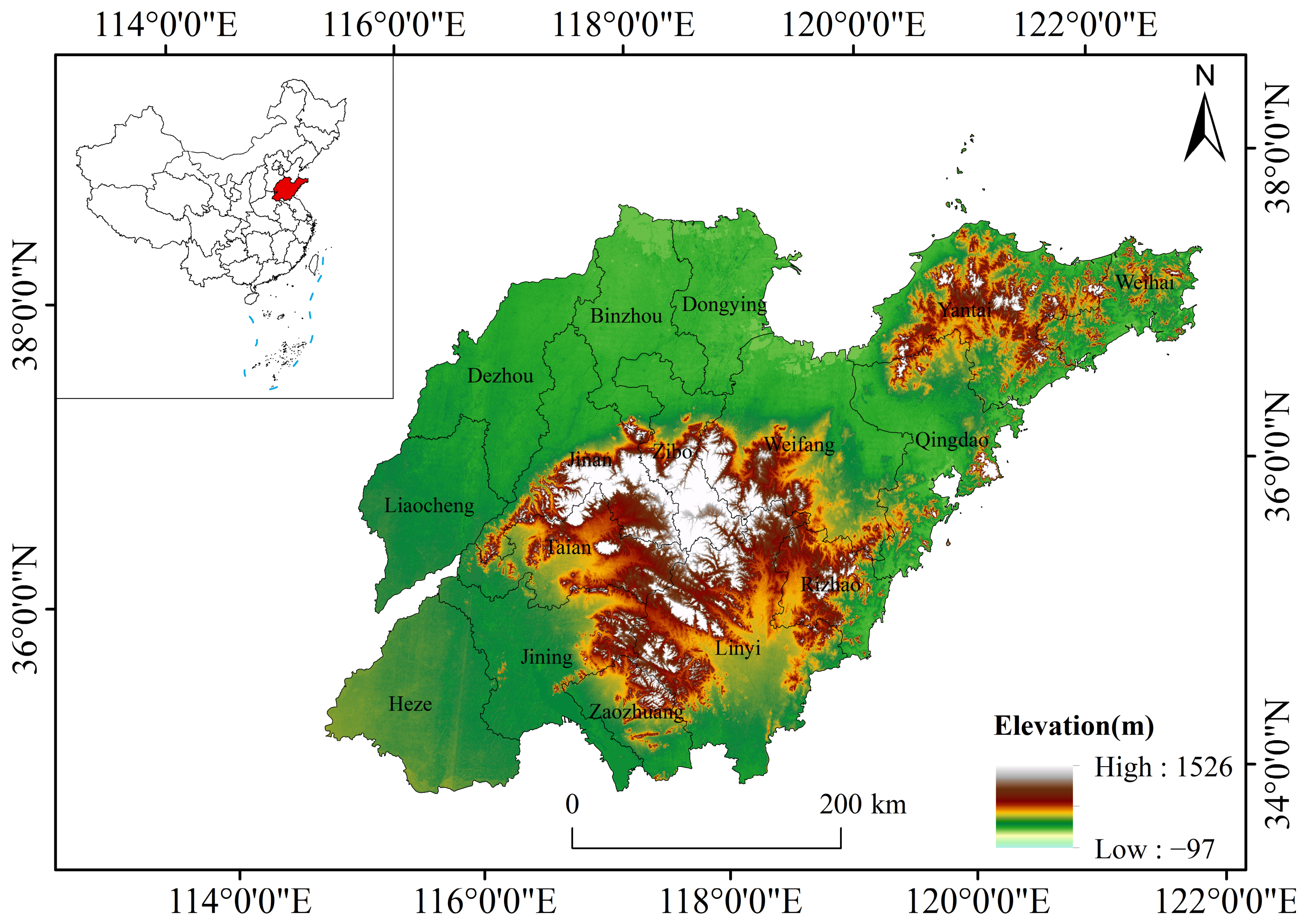
Shandong Province lies on the eastern coast of China and the lower reaches of the Yellow River, with the Yellow Sea to the east and the Bohai Sea to the north. Its geographic extent is 34°22.9′–38°24.01′ N and 114°47.5′–122°42.3′ E (Figure 1). The province occupies a strategic land–sea position that links inland China with coastal economic zones. Plains occupy approximately 66% of Shandong Province and are mainly distributed across western Shandong and the northern coastal region. Hilly areas, accounting for about 15% of the province, are concentrated in the Jiaodong Peninsula and southern Shandong. Mountainous terrain represents roughly 19% of the provincial area and is primarily found in central Shandong and parts of the south.

To ensure spatial comparability and reproducibility, all datasets were projected to the same coordinate system and resampled to a 1 km × 1 km grid before model calculation and spatial analysis. Land-use, climate, NDVI, population density, nighttime light, and human footprint data were matched as closely as possible to the five study years of 2000, 2005, 2010, 2015, and 2020. Relatively stable background variables, including DEM and soil properties, were treated as time-invariant during the study period. Detailed information on these datasets is provided in

Table 1. Data sources.

Data	Sources	Scale	Abbreviation
Elevation	Geospatial Data Cloud (https://www.gscloud.cn/)	30 m	DEM
Population density	Chinese Academy of Sciences Resource and Environment Science Data Center (https://www.resdc.cn)	1 km	POP
Normalized difference vegetation index		250 m	NDVI
Land Use/Land Cover		30 m	LULC
Soil types	Harmonized World Soil Database (https://www.fao.org/soils-portal/so, accessed on 23 March 2025)	1 km	Soil
Annual precipitation	National Earth System Science Data Center (https://www.geodata.cn/)	1 km	PRE
Annual potential evapotranspiration	Qinghai-Tibet Plateau Data Center (https://data.tpdc.ac.cn/)	1 km	PET
Mean annual temperature		1 km	TMP
Nighttime light index		500 m	NIGHTLIGHT
Rainfall erosivity	Calculated from rainfall	1 km	R
Soil erodibility	Calculated from soil database	1 km	K
Human Footprint Index	Mu et al. [37] (https://doi.org/10.6084/m9.figshare.16571064, accessed on 17 June 2025)	1 km	HFP

. For datasets with different original spatial resolutions, resampling or zonal statistics were applied according to data type. Potential uncertainties may arise from differences in data resolution, land-use classification accuracy, interpolation methods, temporal mismatch, and model parameter settings. These uncertainties were considered when interpreting the spatial patterns, driving mechanisms, and trade-offs/synergies relationships of ESs.

2.2. Research Framework

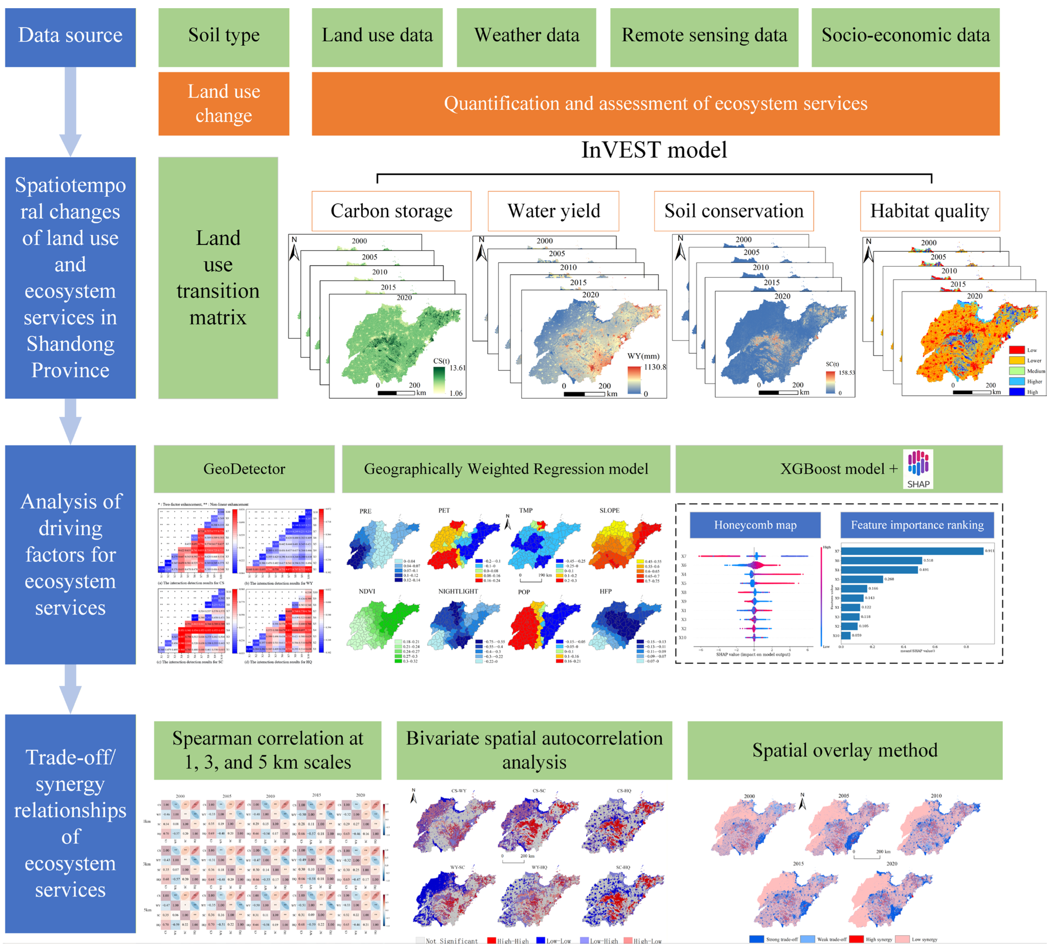
The research framework (Figure 2) integrates multi-scale analysis with multi-method coupling to examine ES interactions and driving mechanisms in Shandong Province. It includes five main steps: (1) quantitatively assessing CS, WY, HQ, and SC with the InVEST model (version 3.14.2); (2) identifying the dominant drivers of each ES using the GeoDetector method implemented in the GD package (version 1.0-5) in R (version 4.5.0); (3) evaluating spatially heterogeneous relationships between drivers and ESs using the GWR module in ArcGIS Pro (version 3.5.4); (4) exploring nonlinear ES responses to drivers using the XGBoost package (version 2.1.1) in Python (version 3.10); and (5) analyzing ES trade-offs and synergies from three perspectives, namely overall correlation, local spatial clustering, and multi-service spatial combinations, using Spearman correlation analysis, bivariate local spatial autocorrelation, and spatial overlay.

2.3. Research Methods

2.3.1. Quantification of ESs

To obtain spatially explicit distribution data for the four key ESs described in this study, the InVEST model was employed to quantify these services; model configuration and parameter calibration procedures are detailed in Appendix A.

2.3.2. Analysis of Driving Factors

(1)

Geodetector

The driving mechanisms underlying the spatial differentiation of ESs in Shandong Province were analyzed using the factor detector and interaction detector modules of GeoDetector. The factor detector was used to quantify the explanatory power of individual driving factors for the spatial differentiation of ESs, while the interaction detector was applied to identify the joint effects of different driving factors. The explanatory power of each driving factor is measured by the q value; a larger q value indicates a stronger ability of the factor to explain the spatial distribution pattern of ESs [38]. The specific formula is as follows:

$$q = 1-{\displaystyle \frac{{\sum }_{h = 1}^L{N}_h{\sigma }_h^2}{N{\sigma }^2}}$$

(1)

Here, h = 1, 2, …, L, where L denotes the stratification of variable Y or factor X, namely classification. N_h and N represent the number of units in stratum h and in the entire study area, respectively. ${\sigma }_h^2$ and σ² denote the variance of Y values in stratum h and in the entire study area, respectively.

(2)

GWR Model

GWR, as a spatial analysis method based on local regression, can better reflect the non-stationarity of variable relationships at different geographical locations [39,40,41]. In this study, the GWR model was employed to examine the spatially varying relationships between ecosystem services and their driving factors, thereby revealing regional differences in the strength and direction of these relationships [42]. The specific formula is as follows:

$$y_i ={ \beta }_0\left(u_i, v_i\right) + {\sum }_{k = 1}^p{\beta }_k\left(u_i,{ v}_i\right)x_{\mathit{ik}} + {\epsilon }_i$$

(2)

Here, y_i denotes the dependent variable at location i, and x_ik represents the k-th independent variable. The spatial coordinates of location i are denoted by (u_i, v_i), and p is the total number of independent variables. The term β₀(u_i, v_i) represents the local intercept at location i, whereas β_k(u_i, v_i) denotes the locally varying regression coefficient of the k-th independent variable at that location. A negative coefficient indicates a negative association, whereas a positive coefficient indicates a positive association.

To ensure the reliability of the GWR results, model diagnostics were conducted and compared with the corresponding OLS model (

Table 2. Comparison of OLS and GWR model parameters for ecosystem services.

	CS		WY		SC		HQ
Model	OLS	GWR	OLS	GWR	OLS	GWR	OLS	GWR
AICc	−127.9705	−149.7316	1196.4286	1123.7856	378.4818	290.1903	−533.915	−593.5852
R2	0.946	0.9737	0.9814	0.9924	0.9748	0.9923	0.9076	0.9615
Adjusted R2	0.9426	0.9616	0.9789	0.9896	0.9732	0.9889	0.9018	0.947

). GWR model performance was evaluated using AICc, R², and adjusted R². Compared with the OLS model, the GWR model showed higher R² and adjusted R² values and lower AICc values, indicating better model fit and stronger explanatory ability. In addition, the spatial distribution of standardized residuals was examined to assess whether systematic spatial clustering remained after model fitting. These diagnostics confirmed that GWR was suitable for capturing the spatial non-stationarity of relationships between ecosystem services and their driving factors in Shandong Province.

(3)

XGBoost

XGBoost is an efficient implementation of the gradient boosting decision tree (GBDT) algorithm, which integrates multiple classification and regression trees (CARTs) to capture complex nonlinear relationships [43]. Compared with traditional GBDT, XGBoost adds second-order derivative information and regularization terms to the objective function, which not only improves computational efficiency, but also helps reduce overfitting risk and enhance the generalization performance of the model. However, machine learning models usually have strong “black box” characteristics, and their internal decision process is not easy to interpret directly, so it is difficult to clearly reveal the specific role of each feature on the prediction results [44]. The specific formula is as follows:

$$\widehat{y_i}={\sum }_{t=1}^T{f}_t\left(x_i\right), f_t\in F$$

(3)

Here, $\widehat{y_i}$ denotes the predicted value of sample i; x_i represents the feature vector of the sample; f_t denotes the t-th regression tree; F is the function space of regression trees; and T represents the total number of trees.

2.3.3. Trade-Offs and Synergies Between ESs

(1)

Spearman analysis

Spearman’s rank correlation analysis is a non-parametric statistical method for evaluating the strength and direction of monotonic associations between paired variables [45]. Because this method does not make strict assumptions regarding the underlying distribution of the data and exhibits relative robustness against outliers, it is frequently employed to evaluate non-linear yet monotonic relationships, as well as ordinal data. The specific formula is as follows:

$$r_s = 1-{\displaystyle \frac{6{\displaystyle {\sum }_{i = 1}^n}{d}_i^2}{n\left(n^2-1\right)}}$$

(4)

In Equation (4), r_s represents the Spearman rank correlation coefficient; n denotes the number of samples; and d_i is the difference between the ranks of the two variables. The value of r_s ranges from [−1, 1].

Synergy and trade-off relations are divided as shown in

Table 3. Division of synergy and trade-off relationships among ESs.

Relationship Type	Coefficient Range	Explanation
Strong synergy	0.5–1	High synergy between services; trends are highly consistent
Moderate synergy	0.3–0.5	Moderate synergy between services
Low synergy	0–0.3	Weak synergy; same direction but small magnitude
Low trade-off	−0.3–0	Weak trade-off; slight conflict between services
Moderate trade-off	−0.5–−0.3	Moderate trade-off; obvious conflict
Strong trade-off	−1–−0.5	High trade-off; services offset or oppose each other

Based on this idea, Spearman correlation analysis was used to quantitatively test the relationship between ESs in Shandong Province, and the statistical reliability of the results was evaluated with significance level.

(2)

Bivariate spatial autocorrelation

In this study, bivariate local spatial autocorrelation analysis was used to examine the spatial association characteristics among different ESs. This method can characterize the local spatial relationship between the values of one service and another service in its neighborhood in a spatial unit, and reveal the spatial heterogeneity and local clustering characteristics of ES relationships. The specific formula is as follows:

$$I_i = z_{x,i}{\displaystyle {\sum }_{j = 1}^n}{\omega }_{\mathit{ij}}{z}_{y,j}$$

(5)

Here, I_i represents the bivariate local spatial autocorrelation index of spatial unit i; z_x,i denotes the standardized value of variable X in spatial unit i; z_y,j denotes the standardized value of variable Y in neighboring spatial unit j; ω_ij is the element of the spatial weight matrix, which is used to describe the adjacency relationship between spatial units i and j; and n represents the total number of spatial units.

(3)

Spatial Overlay Method

The spatial overlay method, a grid-based quantitative approach integrating raster data superposition and combinatorial analysis, was employed to identify trade-offs and synergies among ESs. Key steps included: (1) classifying and standardizing ES supply capacities using natural breaks classification into three tiers (low = 1, medium = 2, high = 3); (2) generating overlaid spatial layers of tier combinations, weighted by their standardized mean values to preserve relative supply differences; and (3) defining interaction typologies—strong trade-offs (one high-tier service with others ≤ medium), weak trade-offs (≥two high-tier services with others ≤ medium), high synergies (all services ≥ medium), and low synergies (all services ≤ medium with ≥ one low-tier).

Through permutation and combination calculation, the spatial overlay results of the four types of ESs yield a total of 81 combination forms (

Table 4. Trade-off and synergy partitioning criteria and supply combination statistics.

Service Relationship	Subcategory	Supply Capacity Combination Statistics	Number of Combinations	Example Combinations
Trade-off	Strong trade-off	1 high, 3 low	4	3111, 1311
		1 high, 1 medium, 2 low	12	3211, 3121
		1 high, 2 medium, 1 low	12	3221, 3122
	Weak trade-off	2 high, 2 low	6	3311, 3131
		2 high, 1 medium, 1 low	12	3321, 3312
		3 high, 1 low	4	3331, 3313
Synergy	High synergy	4 high	1	3333
		3 high, 1 medium	4	3332, 3323
		2 high, 2 medium	6	3322, 3232
		1 high, 3 medium	4	3222, 2322
		4 medium	1	2222
	Low synergy	3 medium, 1 low	4	2221, 2212
		2 medium, 2 low	6	2211, 2121
		1 medium, 3 low	4	2111, 1211
		4 low	1	1111

). High synergies reflect optimal system functionality, whereas low synergies indicate suboptimal coordination with overall service deficiency. This stratification enables systematic identification of spatially explicit service conflicts and mutual enhancement zones.

3. Results

3.1. Land Use Type Changes

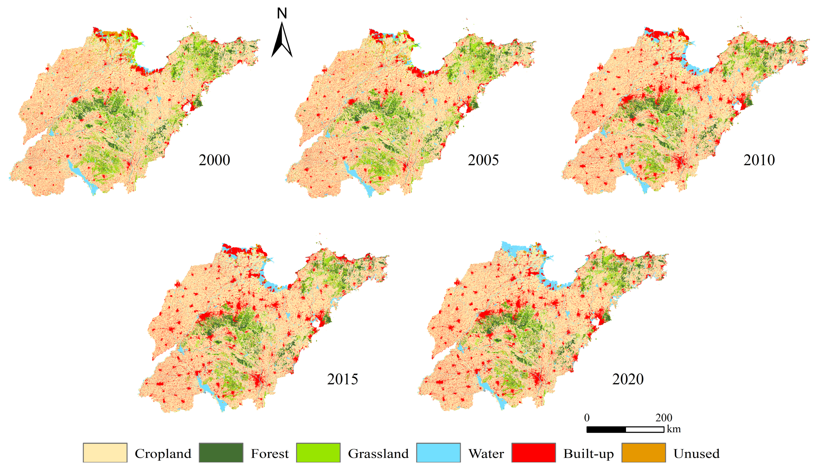
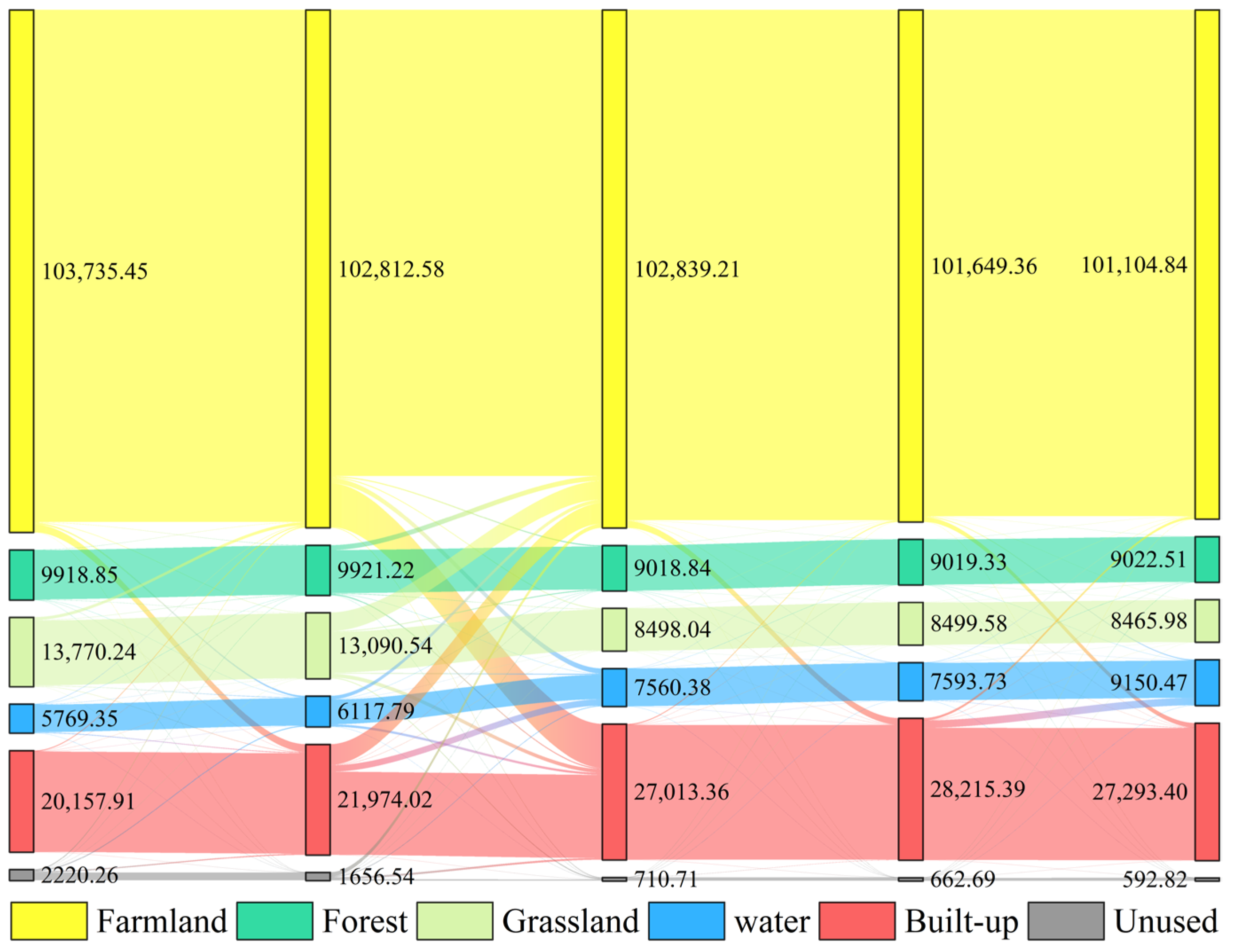
From 2000 to 2020, the land-use pattern of Shandong Province remained generally stable in spatial structure but underwent notable temporal adjustments (Figure 3). Cropland and built-up land were the dominant land-use types, together accounting for approximately 80% of the provincial area (Figure 4). Cropland was the most extensive land-use type, covering almost the entire province, but its area showed a continuous declining trend, decreasing from a peak of 103,735.45 km² in 2000 to 101,104.84 km² in 2020, with the most pronounced reduction occurring between 2010 and 2020. Built-up land was widely distributed across the province and expanded continuously during the study period, particularly around urban fringes, reflecting the encroachment of built-up areas into surrounding agricultural and ecological spaces.

Forest land was mainly concentrated in the central mountainous areas and the eastern hilly regions of Shandong. Its area showed a slight overall decline, reaching a maximum of 9918.85 km² in 2000 and a minimum of 9018.84 km² in 2010. Grassland was primarily distributed in the central-southern mountainous and hilly areas and also exhibited a decreasing trend. In contrast, water bodies expanded gradually, with major distributions in northern and southwestern Shandong, especially along coastal zones and around Laizhou Bay. Overall, land-use change in Shandong Province during 2000–2020 was characterized by cropland contraction, built-up land expansion, grassland reduction, and localized increases in water bodies. The main land-use transitions included the conversion of cropland to built-up land and water bodies, forest land to cropland and built-up land, grassland to cropland and built-up land, and unutilized land to cropland.

3.2. Spatiotemporal Changes in ESs

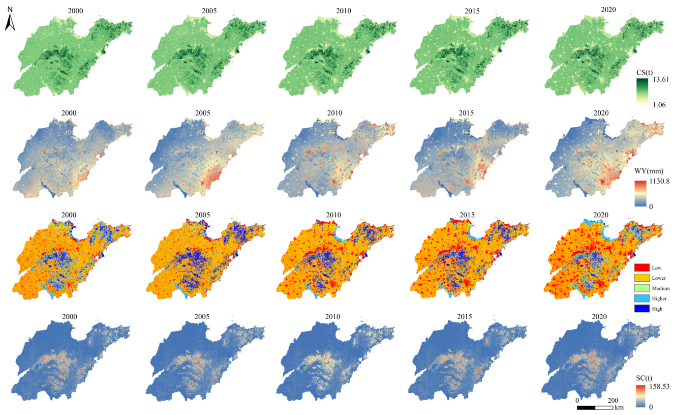
From 2000 to 2020, key ESs in Shandong Province showed substantial spatiotemporal variation under the joint influence of natural conditions and anthropogenic activities (Figure 5). CS showed a slight overall decline, decreasing by 1.8 × 10⁷ t from 15.24 × 10⁸ t in 2000 to 15.06 × 10⁸ t in 2020. This reduction was mainly associated with land-use transitions, particularly the conversion of wetlands, grassland, and cropland into urban and industrial land. Spatially, CS losses were more evident in coastal areas, especially around Laizhou Bay, whereas localized increases occurred in some areas such as Kenli.

WY displayed substantial interannual variation, increasing from 122.81 mm in 2000 to 293.47 mm in 2020. This change was closely related to fluctuations in precipitation, periodic drought events, and land-use intensification. In spatial terms, eastern coastal areas showed a notable net increase in water yield, reaching approximately 14.06 × 10⁸ m³. SC was generally higher in the central mountainous areas and northeastern hilly regions, reaching 12.32 × 10⁸ t in 2020. These areas are characterized by relatively steep slopes and better vegetation cover, which enhance SC capacity. In contrast, plain areas exhibited weaker soil retention due to flat terrain, intensive cultivation, and stronger anthropogenic disturbance.

HQ declined markedly during the study period, decreasing by 12.36% from 0.348 to 0.305. This decline was mainly driven by urban expansion and the encroachment of built-up land into ecological spaces and habitat corridors, particularly around major urban areas such as Jinan and Qingdao. Although ecological conservation efforts after 2015 contributed to partial improvement in some regions, habitat fragmentation remained evident.

3.3. Analysis of Driving Factors of ESs

3.3.1. GeoDetector-Based Assessment of Explanatory Power

GeoDetector places greater emphasis on identifying spatial differentiation characteristics, thus offering certain advantages in explaining the spatial heterogeneity of geographical phenomena. Building on this, this study selected annual precipitation, potential evapotranspiration, annual average temperature, slope, elevation, NDVI, land use/land cover, nighttime light index, population density, and human footprint index as driving factors (

Table 5. Screening of driving factors.

Factor Category	Factor Name	Code
Natural environment factors	Annual Precipitation (PRE)	X1
	Potential Evapotranspiration (PET)	X2
	Annual Mean Temperature (TMP)	X3
	SLOPE	X4
	Elevation (DEM)	X5
	Normalized Difference Vegetation Index (NDVI)	X6
	Land Use/Land Cover (LULC)	X7
Socioeconomic factors	Nighttime Light (NIGHTLIGHT)	X8
	Population Density (POP)	X9
	Human Footprint Index (HFP)	X10

). The factor detection module is utilized to assess the explanatory power of each factor concerning the spatial distribution of ESs.

Based on the detection results of dominant influencing factors using the geographical detector (

Table 6. Influence of driving factors of ESs on the explanatory power q value.

ESs	PRE	PET	TMP	SLOPE	DEM	NDVI	LULC	NIGHTLIGHT	POP	HFP
CS	0.134	0.064	0.279	0.622	0.453	0.231	0.718	0.222	0.237	0.300
WY	0.660	0.270	0.157	0.289	0.227	0.279	0.218	0.144	0.103	0.172
SC	0.348	0.228	0.327	0.931	0.751	0.057	0.514	0.088	0.191	0.217
HQ	0.104	0.186	0.224	0.573	0.391	0.136	0.689	0.292	0.426	0.530

), there are significant differences in the explanatory power of different driving factors for various ESs. This indicates that the spatial differentiation of ESs in Shandong Province is not dominated by a single factor, but is jointly influenced by the natural geographical background, land use pattern, and human activities. Overall, topographic factors and land use factors generally exhibit higher explanatory power, serving as the dominant factors shaping the regional pattern of ESs. In contrast, some climatic factors and socio-economic factors show relatively weaker explanatory power, and their influence is more often reflected as auxiliary effects on local areas or specific service types.

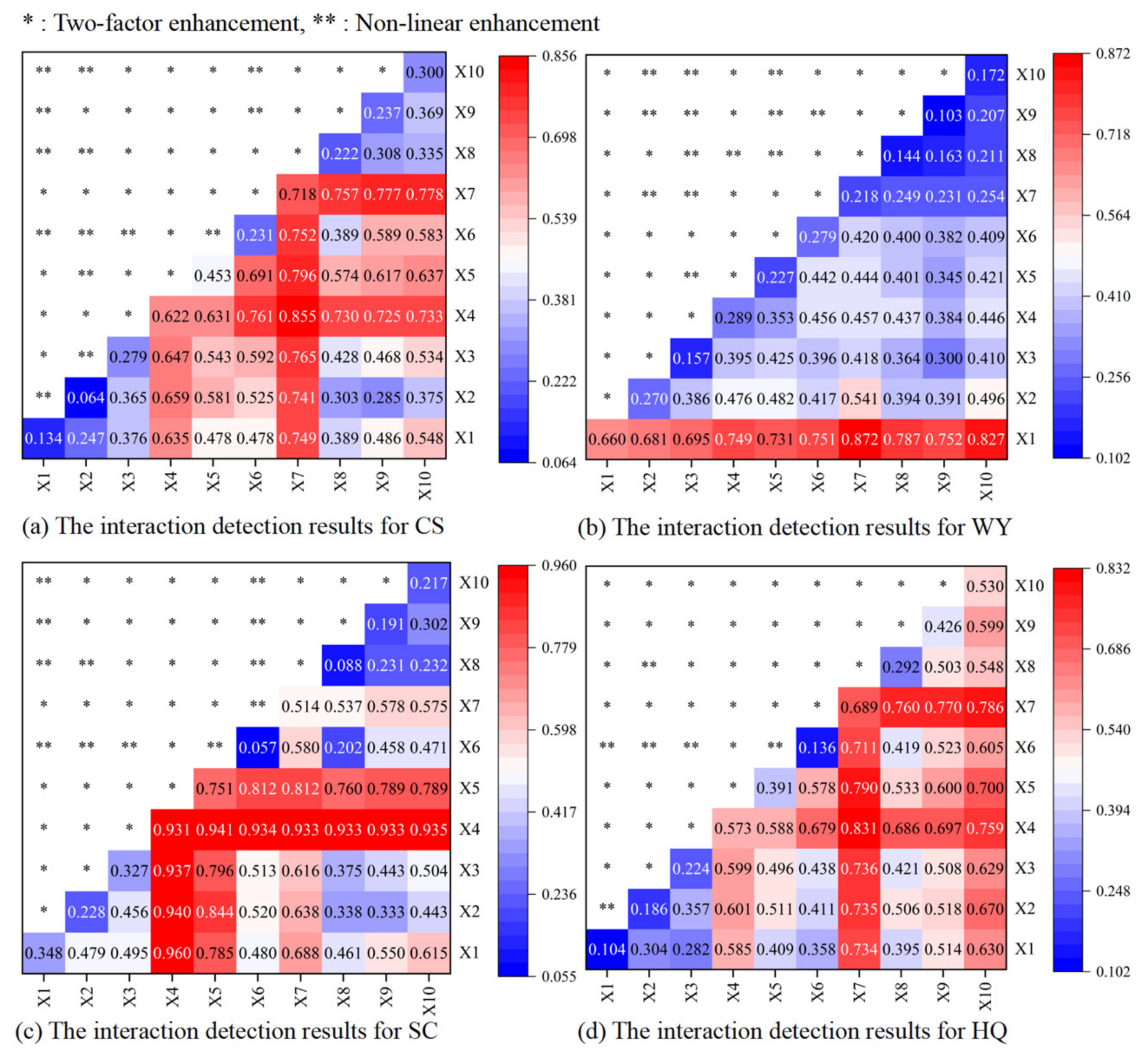
The GeoDetector results showed clear differences in the explanatory power of driving factors among the four ESs (Figure 6). LULC had the highest explanatory power for CS and HQ, while SLOPE and DEM were the dominant factors for SC. WY was mainly explained by PRE. The interaction detector further showed that paired factors generally had stronger explanatory power than individual factors, with the strongest interactions observed for SLOPE ∩ LULC in CS, PRE ∩ LULC in WY, PRE ∩ SLOPE in SC, and SLOPE ∩ LULC in HQ. These results indicate that ES spatial patterns were shaped by both single-factor effects and nonlinear interactions among natural and anthropogenic drivers.

The spatial distribution of ESs revealed distinct interaction mechanisms among driving factors. CS demonstrated prominent high-value interactions between land use and topographic factors, with the X4 ∩ X7 combination achieving the maximum q-value (0.855), indicating that terrain-land use coupling primarily governs carbon spatial patterns through synergistic effects on landscape configuration and anthropogenic pressure. WY exhibited precipitation-dominated interactions, where X1 ∩ X7 attained the peak q-value (0.872), suggesting precipitation acts as the fundamental driver that amplifies spatial heterogeneity when coupled with human activities. Similarly, SLOPE emerged as the critical determinant for SC, evidenced by X1 ∩ X4 interactions reaching q = 0.96, while HQ manifested its strongest interactions (X4 ∩ X7, q = 0.831) through the combined constraints of land use intensification and topographic-mediated development patterns, collectively highlighting the nonlinear amplification of human–natural system interactions in shaping service heterogeneity.

3.3.2. Spatial Heterogeneity Analysis Based on GWR

The initial variable set included PRE, PET, TMP, SLOPE, DEM, NDVI, NIGHTLIGHT, POP, and HFP. DEM was excluded from the final GWR model because its VIF exceeded 10 [46].

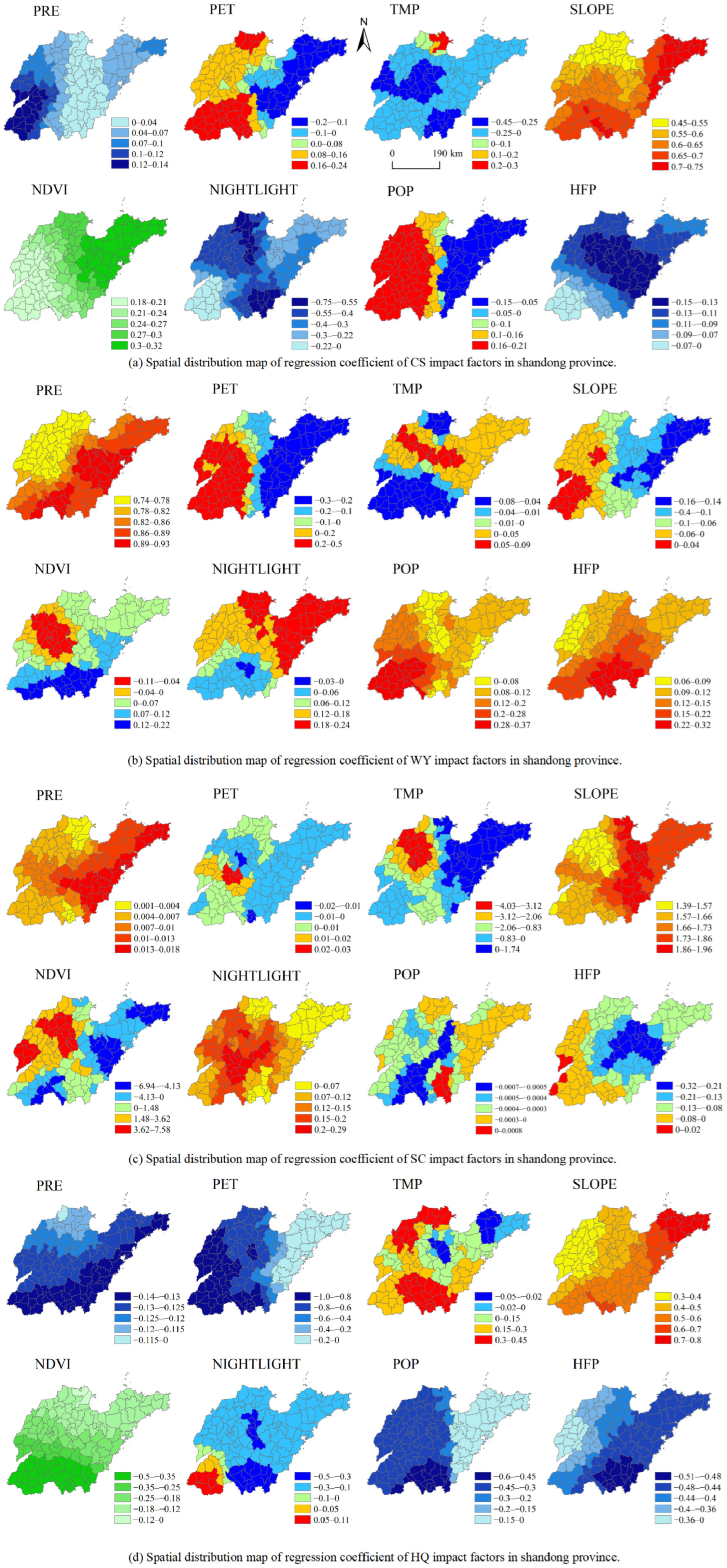
This study revealed pronounced spatial heterogeneity in the driving mechanisms of ESs across Shandong Province (Figure 7). For CS, PRE showed weak positive local regression coefficients, ranging from 0 to 0.14, whereas TMP and PET exhibited region-specific positive and negative effects. In contrast, anthropogenic factors, particularly NIGHTLIGHT (−0.75 to 0) and HFP (−0.15 to −0.07), were predominantly negatively associated with CS, indicating that intensified human activities tend to suppress regional carbon accumulation.

WY was mainly controlled by PRE, with regression coefficients ranging from 0.74 to 0.93, highlighting the dominant role of precipitation in shaping regional hydrological processes. Anthropogenic variables, such as POP, also showed positive effects in some areas, with coefficients ranging from 0.03 to 0.37. This may be related to increased surface runoff caused by urban expansion and the growth of impervious surfaces. By contrast, PET (−0.30 to 0.50) and SLOPE (−0.16 to 0.04) showed spatially varying regression coefficients. This indicates that evapotranspiration demand and terrain-related constraints had heterogeneous, and in some areas relatively weak, effects on WY across Shandong Province.

SC was mainly influenced by natural environmental factors, especially SLOPE, whose regression coefficients ranged from 1.39 to 1.96, substantially exceeding those of PRE (0.001 to 0.018). This indicates that topographic conditions play a key role in regulating SC capacity in Shandong Province. In addition, NDVI (−6.94 to 7.58) and TMP (−4.03 to 1.74) displayed strong spatial non-stationarity, suggesting that vegetation cover and thermal conditions influence SC differently under varying environmental and LULC contexts.

Compared with the other ESs, HQ was more strongly constrained by anthropogenic disturbance. POP showed consistently negative effects on HQ, with coefficients ranging from −0.60 to −0.15, indicating that population concentration and urban expansion may reduce habitat quality by intensifying landscape fragmentation and disrupting ecological corridors. Meanwhile, PRE (−0.14 to 0) and NDVI (−0.50 to −0.12) also showed negative relationships with HQ in some regions, implying potential trade-offs among ESs under specific environmental conditions. Overall, these spatially differentiated driving mechanisms suggest that ecological management in Shandong Province should adopt region-specific strategies rather than uniform policy interventions.

3.3.3. Analysis of Drivers of ESs Using XGBoost–SHAP

In this study, the prediction results of four ESs were systematically analyzed using the XGBoost machine learning algorithm combined with the SHAP interpretability method. SHAP was applied to interpret the outputs of the XGBoost model, quantify the contribution of each driving factor to ES variation, and further reveal the direction and interaction characteristics of their effects.

The predictive performance of the XGBoost models for the four ESs was evaluated using MSE, RMSE, MAE, and R² (

Table 7. Predictive performance of XGBoost models for different ESs.

	Data Subset	MSE	RMSE	MAE	R2
CS	Train (70%)	0.967	0.983	0.667	0.908
	Test (30%)	1.615	1.271	0.802	0.851
WY	Train (70%)	934.721	30.573	22.310	0.884
	Test (30%)	1420.165	37.685	25.988	0.827
SC	Train (70%)	1.600	1.265	0.868	0.981
	Test (30%)	2.686	1.639	1.042	0.968
HQ	Train (70%)	0.002	0.049	0.037	0.919
	Test (30%)	0.003	0.058	0.042	0.891

). The results showed that all models achieved good predictive performance, with testing R² values ranging from 0.827 to 0.968, indicating that XGBoost effectively captured the nonlinear relationships between ecosystem services and their driving factors. Among the four services, SC showed the highest prediction accuracy, with a testing R² of 0.968, followed by HQ and CS, with testing R² values of 0.891 and 0.851, respectively. Water yield showed a relatively lower testing R² of 0.827, which may be attributed to the combined effects of precipitation, evapotranspiration, land use, vegetation cover, and topographic conditions on hydrological processes. Overall, the small differences between training and testing R² values suggest that no obvious overfitting occurred and that the models had good generalization ability.

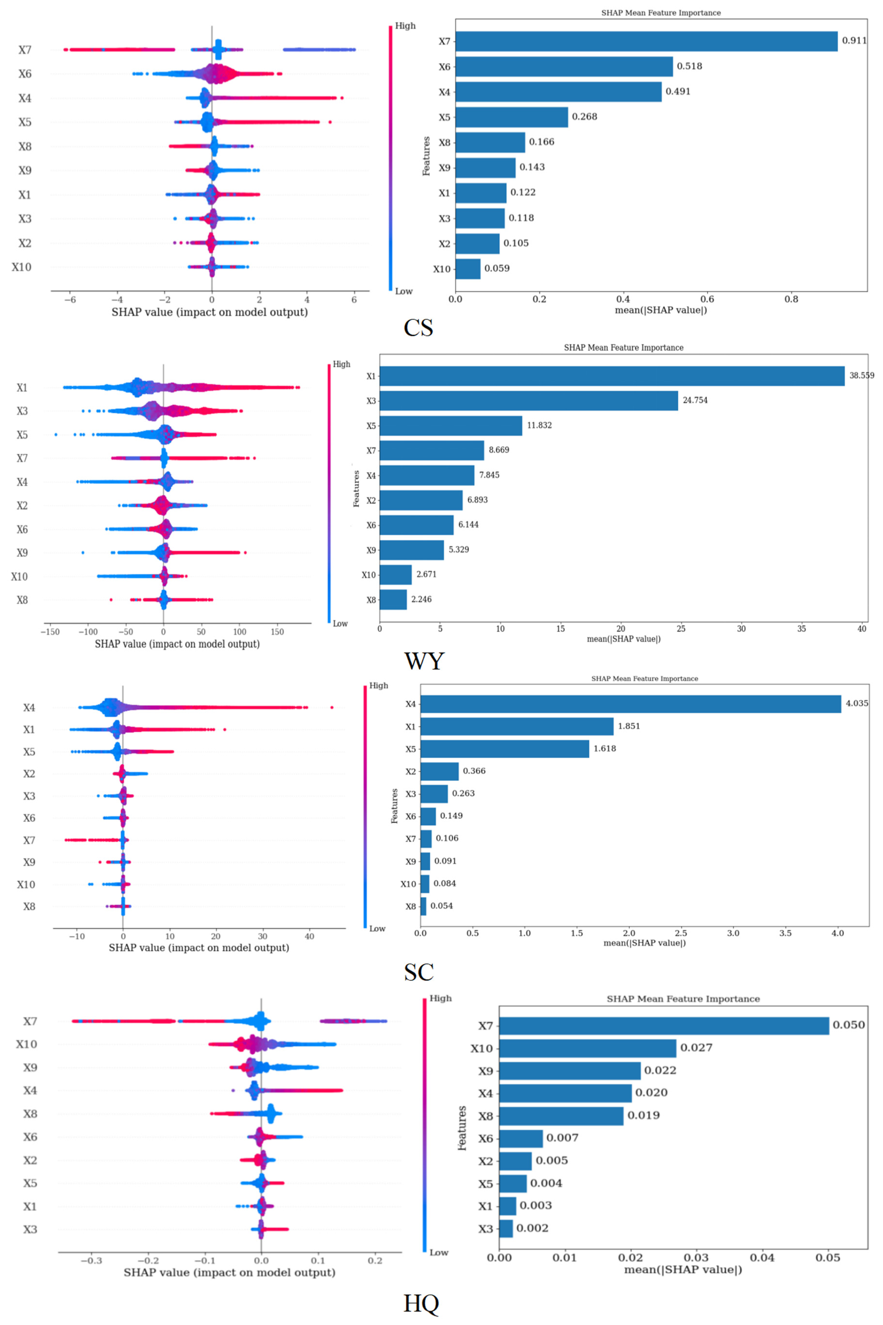
SHAP results revealed heterogeneous positive and negative effects across variables and service types. Specifically, the key determinants of CS were LULC, NDVI, and SLOPE; WY was closely associated with PRE, PET, and SLOPE; SC was primarily driven by SLOPE, PRE, and DEM; and HQ was strongly influenced by LULC, HFP, and POP.

The SHAP feature importance analysis showed clear differences in the relative contributions of driving factors to the four ESs (Figure 8). For CS, LULC and NDVI had the highest mean absolute SHAP values, reaching 0.911 and 0.518, respectively, indicating that they were the two most important predictors of CS. SLOPE and DEM also showed relatively high contributions, with SHAP values of 0.491 and 0.268, respectively. In contrast, the SHAP values of climatic and socioeconomic variables were generally lower than 0.17, suggesting weaker explanatory contributions to CS compared with LULC, NDVI, and topographic factors.

PRE had the highest SHAP value among all driving factors for WY, indicating that precipitation was the primary predictor of water yield in Shandong Province. TMP and DEM were also important contributors, followed by SLOPE and NDVI, which showed moderate explanatory effects. By contrast, POP, HFP, and NIGHTLIGHT contributed relatively little, suggesting that anthropogenic variables were less influential than climatic and topographic factors in explaining the provincial-scale spatial variation in WY.

For SC, SLOPE was the most important driving factor, with a SHAP value of 4.035, accounting for approximately 46.83% of the total contribution. PRE and DEM also contributed substantially, with SHAP values of 1.851 and 1.618, respectively. Together, SLOPE, PRE, and DEM accounted for approximately 87.08% of the total contribution, indicating that SC was mainly explained by topographic and hydroclimatic factors. In contrast, NDVI, LULC, and human activity-related variables had much lower SHAP values, generally below 0.15.

Among the predictors of HQ, LULC had the highest SHAP value (0.050), indicating its dominant influence on HQ. Anthropogenic variables also made notable contributions, with HFP, POP, and NIGHTLIGHT showing SHAP values of 0.027, 0.022, and 0.019, respectively. SLOPE had a similar level of influence, with a SHAP value of 0.020. Overall, the SHAP results indicate that CS was mainly associated with LULC and NDVI, WY was primarily driven by PRE, TMP, and DEM, and SC was strongly influenced by SLOPE, PRE, and DEM. By contrast, HQ was shaped mainly by LULC and anthropogenic disturbance factors.

3.4. Spatial-Temporal Patterns of Trade-Offs/Synergies Between ESs

3.4.1. Spearman’s Rank Correlation Analysis

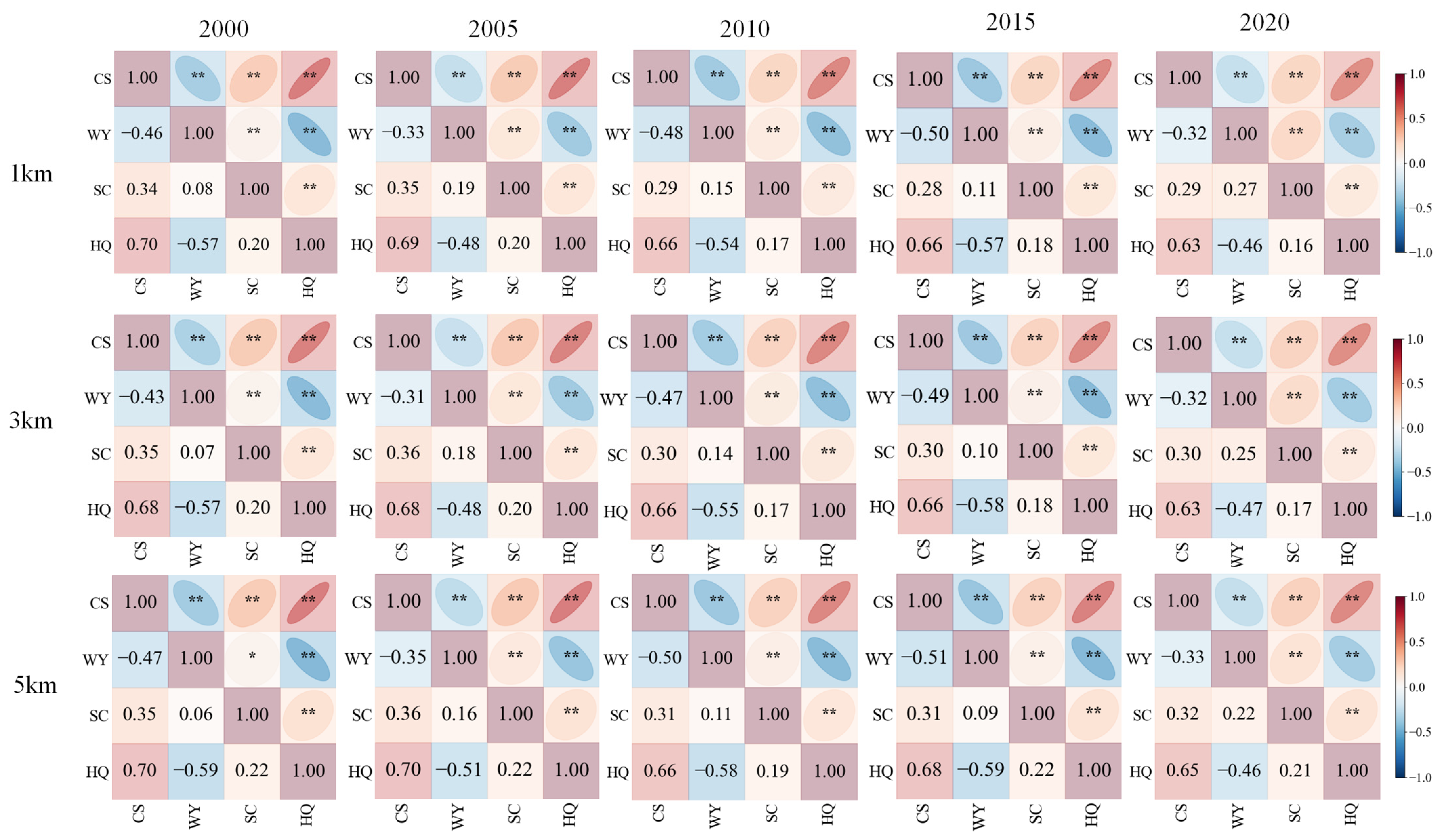
At multiple spatial scales (1, 3, 5 km), ESs in Shandong Province exhibited consistent correlations from 2000 to 2020 (Figure 9). CS and SC were positively associated, though weaker than CS–HQ, indicating that increased vegetation simultaneously enhances carbon sequestration and SC, while topography and rainfall modulate this relationship. WY generally showed negative correlations with CS and HQ, reflecting trade-offs between regulatory services and water provision, particularly in areas with dense vegetation and high ecosystem integrity. Correlation strength varied with spatial scale: CS–HQ synergy remained strong and stable, CS–SC synergy was moderate, and SC–WY and SC–HQ were weakly positive but tended to increase over time. Temporal trends indicated overall stability in correlation directions, with gradual adjustments in strength due to land use changes, urbanization, ecological restoration, and water management interventions. Notably, negative trade-offs between water provision and regulatory services slightly weakened over time, while couplings between WY and SC strengthened, highlighting the influence of ecosystem management on ES interactions.

3.4.2. Bivariate Local Spatial Autocorrelation Analysis

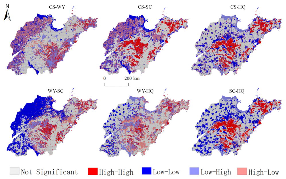
This study adopts a 1 km grid as the basic evaluation unit to reveal the spatial heterogeneity of ESs at a fine scale. To quantitatively identify spatial association patterns among different ESs, a bivariate local spatial autocorrelation analysis method was implemented using GeoDa software (version 1.22.0.21). This approach precisely detects the degree of spatial association between one ES at a specific location and another service at adjacent spatial locations. The results were visualized through LISA (Local Indicators of Spatial Association) cluster maps, categorized into four cluster types: High–High (H–H) and Low–Low (L–L) clusters (indicating synergy relationships), and High–Low (H–L) and Low–High (L–H) clusters (representing trade-off relationships).

Bivariate local Moran’s I was used to identify local spatial coupling among CS, WY, SC, and HQ (Figure 10). The proportion of non-significant units ranged from 45.35% to 59.76% across service pairs, indicating that bivariate spatial associations are mainly concentrated in specific topographic and land-use sensitive areas. Pairs involving HQ showed higher non-significance (59.76%) than CS–WY (47.53%), CS–SC (45.35%) and WY–SC (45.35%), suggesting more active local coupling among the latter three.

For CS–WY, positive and negative associations coexisted: low–low (16.27%), high–high (9.93%), low–high (13.29%) and H–L (12.98%). CS–SC was dominated by positive associations (L–L 23.48%, H-H 13.90%; L-H only 1.87%). CS–HQ also showed positive association (L–L 17.16%, H–H 13.27%) with few mismatch types. WY–SC exhibited the strongest low–low dominance (31.09%, the highest among all pairs). WY–HQ showed pronounced spatial mismatch. SC–HQ displayed strong positive association. Spatially, high–high clusters were mainly located in the central-southern hilly areas and Jiaodong Peninsula, while low–low clusters dominated the northwestern and southwestern plains, reflecting the influence of natural background and human activity intensity.

3.4.3. Spatial Overlay Analysis

Spatial overlay analysis was conducted to identify trade-off and synergistic relationships among ESs in the study area. These relationships were further grouped into four categories: strong trade-off, weak trade-off, high synergy, and low synergy. Through permutation and combination calculations, the spatial overlay of the four ESs yielded a total of 81 unique combination patterns. The composite spatial overlay code was calculated as follows:

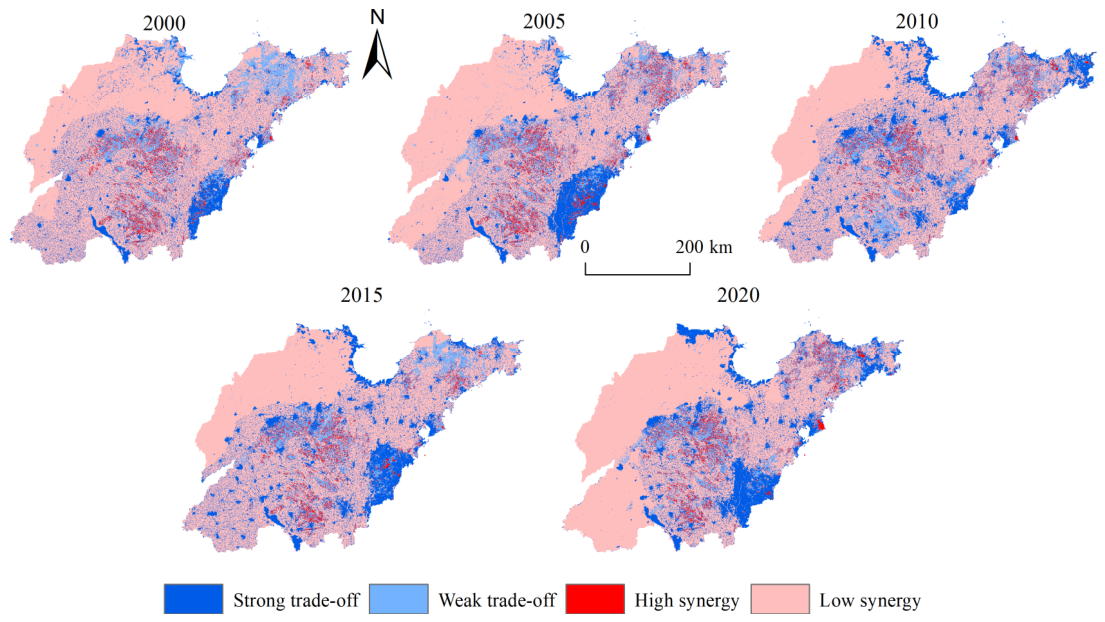
From 2000 to 2020, the ES relationships in Shandong Province were mainly characterized by low-synergy and strong-trade-off patterns (Figure 11), in which low synergy is mainly distributed in the northwest plain of Shandong Province; strong trade-off is mainly distributed in Lanshan District, Donggang District, Wulian County and other areas as well as coastal area of Laizhou Bay, especially in some coastal counties and areas with high urbanization degree; weak trade-off area mainly presents patch and strip distribution, which is common in Jiaodong Peninsula, coastal zone and central Shandong area; the distribution of high synergy area is the least, and the whole distribution is scattered dot or small patch mosaic, mainly scattered in some areas of central and southern Shandong Province and some areas with good ecological background.

From 2000 to 2020, interactions among ESs in Shandong Province were predominantly characterized by low-synergy and strong trade-off patterns, with clear spatial heterogeneity (

Table 8. The changes in ecosystem trade-offs and synergies in Shandong Province from 2000 to 2020.

Year	Relationship	Area (km2)	Percentage of Total Area (%)	Year	Relationship	Area (km2)	Percentage of Total Area (%)
2000	Strong trade-off	22,722.22	14.68	2015	Strong trade-off	31,401.17	20.28
	Weak trade-off	16,704.90	10.79		Weak trade-off	11,634.98	7.51
	High synergy	5561.11	3.59		High synergy	4608.99	2.98
	Low synergy	109,829.05	70.94		Low synergy	107,182.04	69.23
2005	Strong trade-off	24,496.54	15.82	2020	Strong trade-off	28,692.08	18.54
	Weak trade-off	15,055.36	9.72		Weak trade-off	10,799.73	6.98
	High synergy	6821.76	4.41		High synergy	5532.56	3.57
	Low synergy	108,440.02	70.05		Low synergy	109,732.74	70.91
2010	Strong trade-off	29,790.46	19.24
	Weak trade-off	11,515.78	7.44
	High synergy	4591.82	2.97
	Low synergy	108,931.91	70.36

). Low-synergy zones were the dominant interaction type throughout the study period, accounting for 69.23–70.94% of the total area. These zones were mainly distributed in the northwestern plains, where multiple ESs generally remained at moderate levels and showed relatively weak mutual enhancement.

Strong-trade-off zones showed an overall expansion trend, increasing from 22,722.22 km² in 2000 to 31,401.17 km² in 2015, followed by a slight decline by 2020. Spatially, these zones were mainly concentrated in coastal areas, such as Lanshan, Donggang, and Wulian, as well as in more urbanized regions. This pattern indicates that conflicts among ESs became more pronounced in areas affected by intensive land-use competition and human disturbance. Weak-trade-off zones exhibited a more scattered distribution and decreased from 16,704.90 km² in 2000 to 10,799.73 km² in 2020. Spatially, these zones were concentrated in the Jiaodong Peninsula and central-southern Shandong, where they served as transitional areas between strong trade-off and low-synergy zones. High-synergy zones remained limited during the study period, accounting for only 2.97–4.41% of the total area. These zones were generally fragmented and distributed as small patches in the southern regions with relatively better ecological conditions.

4. Discussion

4.1. Driving Mechanisms of ESs

The spatial differentiation of ESs in Shandong Province was driven by coupled natural and anthropogenic processes. The GeoDetector results showed that individual ESs had distinct dominant drivers. LULC had the strongest explanatory power for CS and HQ, precipitation was the dominant factor for WY, and topographic variables, especially SLOPE and DEM, had the strongest influence on SC. These findings indicate that different ESs are controlled by different ecological processes and should not be interpreted through a single-factor framework. Recent studies have also emphasized that ES relationships are shaped by both shared drivers and service-specific drivers, and that separating ES relationship analysis from driver analysis may lead to fragmented interpretations [47,48]. LULC was the primary factor shaping CS and HQ because land-cover structure directly determines vegetation biomass, carbon density, habitat suitability, and the degree of ecological disturbance. Forestland and grassland generally support higher carbon sequestration and better habitat conditions, whereas built-up land and intensively used cropland reduce ecological connectivity and increase landscape fragmentation. The strong influence of LULC on CS and HQ also suggests that land-use optimization is central to improving ecological regulation and habitat maintenance in Shandong Province. This is supported by recent Shandong-based evidence showing that built-up land expansion and ecological land conversion can reduce both CS and HQ [49,50].

WY was mainly controlled by precipitation, which is consistent with the basic water-balance mechanism of WY formation. Precipitation provides the primary water input, while evapotranspiration, vegetation cover, soil characteristics, and topography regulate the conversion of precipitation into WY. The strong interaction between precipitation and LULC indicates that hydrological services are not solely climate-driven; rather, they are produced by the coupling of climatic inputs and land-surface hydrological responses. Similar findings have been reported in the Yellow River Basin, where WY was mainly influenced by precipitation, while SC was jointly affected by slope and land-use type [51,52]. SC was predominantly controlled by SLOPE and DEM. This reflects the key role of terrain in regulating soil erosion, runoff velocity, sediment transport, and sediment retention. In mountainous areas, steeper slopes increase erosion potential, but vegetation cover and conservation measures may enhance soil retention. In plains, erosion intensity is generally lower, but intensive cultivation and soil disturbance may weaken SC functions. Therefore, the strong explanatory power of topographic factors does not merely indicate terrain effects, but reflects the interaction between slope-controlled erosion processes and land-surface management [53,54].

Human activity-related factors, including HFP, POP, and NIGHTLIGHT, exerted particularly important effects on HQ and also influenced CS. These factors represent population concentration, urban expansion, infrastructure development, and overall disturbance intensity. Their effects suggest that habitat degradation in Shandong Province is not only caused by direct land-cover conversion, but also by the broader fragmentation, isolation, and disturbance of ecological spaces associated with socioeconomic development. Recent social–ecological framework studies also indicate that ES relationships are shaped by the combined effects of resource systems, governance systems, and stakeholder-related human activities.

The interaction detector showed that paired factors generally had stronger explanatory power than individual factors, indicating that ES patterns were shaped by nonlinear factor interactions. For CS, the interaction between SLOPE and LULC produced the strongest explanatory power, suggesting that terrain and land use jointly determine vegetation distribution and carbon accumulation. For WY, the interaction between precipitation and LULC was dominant, reflecting the coupling between climatic water input and land-surface hydrological response. For SC, the interaction between precipitation and SLOPE was particularly strong, indicating that rainfall erosivity and terrain jointly control soil erosion and retention processes. For HQ, the interaction between SLOPE and LULC highlighted the combined influence of topographic constraints and human land-use intensity on habitat conditions.

The GWR results further revealed spatial non-stationarity in ES driving mechanisms. The same factor could have different coefficient directions and magnitudes across counties, suggesting that regional context modifies the effect of driving factors. For example, human activity variables generally showed negative associations with CS and HQ, but the strength of these effects varied across urban, coastal, mountainous, and agricultural areas. This confirms that uniform ecological policies may be insufficient for Shandong Province and that differentiated regional strategies are necessary.

The use of XGBoost-SHAP provides additional support for identifying nonlinear driver contributions and interpreting complex ES trade-off mechanisms, especially where natural and anthropogenic factors interact nonlinearly [55,56]. LULC and NDVI were the most important predictors of CS, PRE was the dominant predictor of WY, SLOPE and DEM were the key predictors of SC, and LULC together with HFP, POP, and NIGHTLIGHT exerted strong effects on HQ. Recent studies have demonstrated that XGBoost-SHAP can effectively capture nonlinear relationships, identify the direction and magnitude of driver contributions, and improve the interpretability of ES trade-off and synergy mechanisms. Compared with traditional regression or single-factor detection, XGBoost-SHAP better captures nonlinear responses and ranks variable contributions, while GWR reveals spatial heterogeneity and GeoDetector identifies interaction effects. The integration of these methods therefore provides a more comprehensive interpretation of ES driving mechanisms from the perspectives of explanatory power, spatial non-stationarity, and nonlinear response.

4.2. Trade-Offs and Synergies Among Ecosystem Services

The results indicate that interactions among ESs in Shandong Province were characterized by persistent synergies and pronounced spatially heterogeneous trade-offs. Among the examined service pairs, the CS–HQ synergy was the most stable and prominent throughout the study period. This relationship can be primarily attributed to their shared dependence on land-cover composition, vegetation structure, ecological connectivity, and the intensity of anthropogenic disturbance [57]. Forestland and grassland, mainly distributed in the central-southern mountainous region and the Jiaodong hilly areas, generally maintain higher vegetation biomass, more stable carbon pools, greater landscape connectivity, and lower levels of habitat fragmentation [58]. These landscape characteristics simultaneously enhance carbon accumulation and provide suitable ecological conditions for species survival and habitat maintenance. Conversely, urban expansion and the conversion of ecological land into cropland or construction land can weaken carbon sequestration capacity and degrade habitat suitability. Therefore, the CS–HQ synergy reflects a shared ecological response to land-use intensity, vegetation cover, and landscape fragmentation, rather than an incidental statistical association. This mechanism is consistent with recent findings from Shandong Province, which emphasize the common sensitivity of CS and HQ to land-use conversion and built-up land expansion [59].

The positive correlation between CS and SC further highlights the role of vegetation-mediated regulating processes. Vegetation enhances carbon sequestration through the accumulation of aboveground biomass, belowground biomass, and soil organic carbon, while simultaneously reducing soil erosion by intercepting rainfall, stabilizing soil aggregates, increasing surface roughness, and slowing surface runoff. However, the synergy between CS and SC was weaker than that between CS and HQ, suggesting that SC is not controlled by vegetation alone. In mountainous and hilly regions, slope, elevation, rainfall erosivity, and sediment transport processes largely determine erosion intensity and sediment redistribution. Therefore, the ecological linkage between CS and SC may vary substantially under different topographic and hydroclimatic conditions. Similar synergistic relationships between vegetation-mediated CS and SC have also been reported in vegetation restoration regions such as the Loess Plateau, where ecological restoration and the Grain for Green Program improved vegetation cover, enhanced carbon sequestration, reduced soil erosion, and strengthened the synergy between regulating ecosystem services [60,61]. These findings indicate that vegetation restoration can simultaneously improve carbon fixation and soil retention capacity, but the strength of this synergy is likely to be modulated by terrain and climate conditions.

In contrast, WY exhibited trade-offs with both CS and HQ, especially with HQ, reflecting the divergent ecological processes underlying provisioning and regulating services. Areas with dense vegetation and high habitat integrity usually have stronger canopy interception, root water uptake, and evapotranspiration, which may reduce the proportion of precipitation converted into surface runoff or WY [62,63,64]. Conversely, cropland and built-up land may generate relatively higher runoff because of lower vegetation water consumption or increased impervious surfaces, but these land-use types generally have lower CS and poorer habitat conditions. Thus, the WY–CS and WY–HQ trade-offs arise from the mismatch between runoff-generation processes and vegetation-mediated ecological regulation. These relationships are not merely statistical correlations, but reflect the tension between hydrological output and ecological regulation under different land-cover and vegetation conditions [65]. This interpretation is consistent with recent studies indicating that increased vegetation cover can enhance CS, HQ, and SC, while potentially reducing WY through higher evapotranspiration and interception [66,67,68].

The bivariate local spatial autocorrelation and spatial overlay results further confirmed that ES relationships were spatially non-uniform. Positive spatial associations were mainly observed in mountainous and hilly regions with relatively intact ecological structures, whereas trade-off patterns were more common in urban expansion zones, coastal development areas, and intensively cultivated plains. This finding supports the view that ES trade-offs and synergies are scale-dependent and spatially heterogeneous, and that the same ES pair may exhibit different or even opposite relationships across different spatial units [69]. Therefore, global correlation coefficients alone cannot fully capture the spatial complexity of ESs interactions.

The spatial overlay analysis showed that low-synergy areas consistently dominated Shandong Province, accounting for approximately 69.23–70.94% of the study area. This indicates that most regions did not achieve the coordinated high-level provision of multiple ESs. Low-synergy areas were mainly distributed in the northwestern and southwestern plains, where intensive cropland, flat terrain, and expanding built-up land limited the simultaneous enhancement of CS, HQ, and SC. Although these areas may maintain certain provisioning or runoff-generation functions, their capacities for CS, habitat maintenance, and SC are relatively constrained. Strong trade-off areas expanded overall during the study period and were mainly concentrated in urbanizing and coastal areas, including parts of Laizhou Bay and highly developed counties. By contrast, high-synergy areas remained spatially limited and were mainly scattered in the central-southern mountainous region and the Jiaodong Peninsula, where favorable terrain, relatively high vegetation cover, and lower human disturbance support the coordinated provision of multiple ESs.

Overall, trade-off and synergy relationships among ESs in Shandong Province reflect the combined effects of land-use structure, vegetation condition, topographic differentiation, and human disturbance. The stable CS–HQ synergy indicates that ecological conservation and land-use regulation in mountainous and hilly areas are essential for maintaining multifunctional ecological benefits. The relatively weak CS–SC synergy suggests that soil conservation management should account for terrain conditions and rainfall erosivity, rather than relying solely on vegetation restoration. Trade-offs between WY and vegetation-related regulating services further imply that ecological restoration should balance vegetation enhancement with regional water availability, particularly in water-limited areas. These findings provide a scientific basis for differentiated ecological management. Specifically, mountainous and hilly areas should prioritize ecological conservation and connectivity maintenance, whereas plains, rapidly urbanizing regions, and coastal zones should focus on controlling built-up land expansion, optimizing landscape structure, and mitigating ES trade-offs.

4.3. Management Implications

The findings provide several implications for ecological conservation, land-use optimization, and regional sustainable development in Shandong Province [70]. First, the central-southern mountainous region and the Jiaodong hilly areas should be prioritized as key ecological conservation zones. These areas play a crucial role in maintaining CS–HQ synergy and supporting multi-service stability. Management efforts should focus on protecting forestland and grassland, maintaining ecological corridors, improving habitat connectivity, and preventing the further conversion of ecological land into built-up land. Second, ecological restoration in the northwestern and southwestern plains should emphasize multi-service coordination rather than the enhancement of a single ES. These regions are dominated by cropland, flat terrain, and relatively intensive human activities, which constrain CS, HQ, and SC. Therefore, ecological management should promote farmland shelterbelts, riparian buffers, ecological ditches, small wetlands, and mosaic ecological patches. These measures can improve habitat connectivity, increase carbon sequestration potential, and enhance soil retention while maintaining agricultural production. Third, in rapidly urbanizing areas and coastal zones, strict control of ecological land conversion is necessary to mitigate strong trade-offs between urban development and ecosystem conservation. Built-up land expansion should be coordinated with blue–green infrastructure planning, ecological redline protection, and habitat restoration. In coastal areas such as Laizhou Bay, particular attention should be given to the protection and restoration of wetlands, estuarine habitats, and coastal ecological buffer zones, because these areas are highly sensitive to land-use change and provide important regulating and supporting services. Overall, ecological management in Shandong Province should shift from single-service optimization toward spatially differentiated multi-service governance. Mountainous and hilly areas should be managed as ecological conservation and synergy-maintenance zones; plain agricultural areas should be treated as ecological function enhancement zones; and coastal and urbanizing regions should be regulated as trade-off control zones. Such a differentiated zoning strategy would help improve the coordination of ESs under continued urbanization, agricultural intensification, and climate variability.

4.4. Limitations and Future Research

Several limitations should be acknowledged. First, although the 1 km grid resolution is appropriate for provincial-scale analysis, it may not fully capture fine-scale ecological processes in urban fringes, coastal wetlands, river corridors, and fragmented habitat patches. Future studies should incorporate higher-resolution remote sensing data and finer spatial units to improve the identification of local ES heterogeneity. Second, the InVEST model involves simplified assumptions and parameter settings. Parameters such as carbon density, biophysical coefficients, threat weights, and habitat sensitivity values may vary across space and time, but they were treated as relatively fixed in this study. Future research should incorporate field observations, local empirical datasets, and parameter sensitivity analysis to reduce model uncertainty and improve assessment accuracy. Third, this study focused mainly on historical ES changes from 2000 to 2020 and did not conduct future scenario simulations. Future studies could combine land-use simulation models, climate change scenarios, and policy intervention scenarios to evaluate how different development pathways may influence ES trade-offs and synergies. Finally, GeoDetector, GWR, and XGBoost-SHAP provide useful tools for examining factor explanatory power, spatially varying relationships, and nonlinear variable contributions. However, these methods primarily capture statistical associations and cannot fully establish causality. Future research should combine process-based modelling, long-term observational data, and causal inference methods to better reveal the mechanisms by which land-use change, climate variability, and human activities shape interactions among ESs.

5. Conclusions

Based on multi-period remote sensing, meteorological, soil and socio-economic data from 2000 to 2020, this study employed various methods such as the InVEST model, spatial statistics, GeoDetector, GWR, XGBoost-SHAP to systematically analyze the spatiotemporal evolution characteristics, driving mechanisms, and trade-off/synergy relationships of four ESs in Shandong Province, namely CS, HQ, WY, and SC. The main conclusions are as follows:

From 2000 to 2020, the overall land use pattern in Shandong Province remained stable, but structural changes were evident. The cultivated land area decreased from 103,735.45 km² to 101,104.84 km², while built-up land continued to expand, with an influx area of 12,819.75 km², mainly originating from cultivated land. The water surface increased to some extent, while grassland area shrank. Land use transitions mainly involved the conversion of cultivated land to built-up land and water surface, as well as the conversion of grassland to cultivated land and built-up land. Land use change serves as an important prerequisite for the evolution of regional ES patterns.

The dominant factors for CS and HQ were land use type (q values of 0.718 and 0.689, respectively) and topography (SLOPE with q values of 0.622 and 0.573), with human activities (HFP, POP) also exerting significant influences. The dominant factor for WY was annual precipitation (q = 0.660), followed by SLOPE (0.289) and NDVI (0.279). For SC, the dominant factors were SLOPE (q = 0.931) and elevation (0.751), followed by land use (0.514). Interaction detection revealed that two-factor enhancement effects were common, with, for example, the explanatory power of SLOPE ∩ land use for CS reaching 0.855, precipitation ∩ land use for WY reaching 0.872, and precipitation ∩ SLOPE for SC reaching as high as 0.960. GWR and XGBoost-SHAP further revealed the spatial heterogeneity and nonlinear characteristics of the intensity of driving factors.

CS and HQ consistently exhibited a strong synergy, with Spearman correlation coefficients ranging from 0.63 to 0.7. CS showed a moderate synergy with SC (0.28–0.36), while WY showed negative correlations with HQ (−0.46 to −0.59) and with CS (−0.32 to −0.52). Bivariate local spatial autocorrelation indicated that high–high synergy areas were concentrated in the mountainous region of central-southern Shandong and the Jiaodong Peninsula, whereas low–low synergy areas were distributed across the northwestern Shandong Plain. High–low and low–high clusters were more prominent for the WY-HQ pair. Spatial overlay analysis revealed that the proportion of low-synergy areas consistently ranged from 69.23% to 70.94% during the study period. The area of strong trade-offs increased from 22,722.22 km² to 28,692.08 km², whereas high-synergy areas accounted for only 2.97% to 4.41%. These findings indicate that the overall coordination level of ESs in Shandong Province remains low, leaving substantial room for synergy improvement.

References

1. Daily, G.; Postel, S.; Bawa, K.; Kaufman, L. Nature’s Services: Societal Dependence on Natural Ecosystems. In Bibliovault OAI Repository; The University of Chicago Press: Chicago, IL, USA, 1997. [Google Scholar]
2. Xie, G.; Zhang, C.; Zhen, L.; Zhang, L. Dynamic changes in the value of China’s ecosystem services. Ecosyst. Serv. 2017, 26, 146–154. [Google Scholar] [CrossRef]
3. Liu, H.; Zhu, J.; Zeng, L.; Chen, B.; Xiao, W. How to Bridge the Gap? integrating ecosystem service flows to optimize resource allocation in rapidly Urbanizing regions. Ecol. Indic. 2025, 181, 114402. [Google Scholar] [CrossRef]
4. Chen, S.; Liu, X.; Yang, L.; Zhu, Z. Variations in Ecosystem Service Value and Its Driving Factors in the Nanjing Metropolitan Area of China. Forests 2023, 14, 113. [Google Scholar] [CrossRef]
5. Zhang, H.; Liu, S. Exploring the spatial–temporal patterns of urban ecosystem service relationships and their driving mechanisms: A case study of Wuhu City, China. Ecol. Indic. 2024, 167, 112726. [Google Scholar] [CrossRef]
6. Shen, J.; Li, S.; Wang, H.; Wu, S.; Liang, Z.; Zhang, Y.; Wei, F.; Li, S.; Ma, L.; Wang, Y.; et al. Understanding the spatial relationships and drivers of ecosystem service supply-demand mismatches towards spatially-targeted management of social-ecological system. J. Clean. Prod. 2023, 406, 136882. [Google Scholar] [CrossRef]
7. Shao, Y.; Xiao, Y.; Sang, W. Land use trade-offs and synergies based on temporal and spatial patterns of ecosystem services in South China. Ecol. Indic. 2022, 143, 109335. [Google Scholar] [CrossRef]
8. Feng, X.; Fu, B.; Piao, S.; Wang, S.; Ciais, P.; Zeng, Z.; Lü, Y.; Zeng, Y.; Li, Y.; Jiang, X.; et al. Revegetation in China’s Loess Plateau is approaching sustainable water resource limits. Nat. Clim. Change 2016, 6, 1019–1022. [Google Scholar] [CrossRef]
9. Zhang, Z.; Liu, Y.; Wang, Y.; Liu, Y.; Zhang, Y.; Zhang, Y. What factors affect the synergy and tradeoff between ecosystem services, and how, from a geospatial perspective? J. Clean. Prod. 2020, 257, 120454. [Google Scholar] [CrossRef]
10. Fang, L.; Wang, L.; Chen, W.; Sun, J.; Cao, Q.; Wang, S.; Wang, L. Identifying the impacts of natural and human factors on ecosystem service in the Yangtze and Yellow River Basins. J. Clean. Prod. 2021, 314, 127995. [Google Scholar] [CrossRef]
11. Liu, M.; Zhao, S. Spatial Assessment of Ecosystem Services in Zhoushan Archipelago Based on InVEST Model. Sustainability 2025, 17, 3913. [Google Scholar] [CrossRef]
12. Huang, L.; Du, Y.; Tang, Y. Ecosystem service trade-offs and synergies and their drivers in severely affected areas of the Wenchuan earthquake, China. Land Degrad. Dev. 2024, 35, 3881–3896. [Google Scholar] [CrossRef]
13. Tenerelli, P.; Demšar, U.; Luque, S. Crowdsourcing indicators for cultural ecosystem services: A geographically weighted approach for mountain landscapes. Ecol. Indic. 2016, 64, 237–248. [Google Scholar] [CrossRef]
14. Luo, H.; Wang, C.; Li, C.; Meng, X.; Yang, X.; Tan, Q. Multi-scale carbon emission characterization and prediction based on land use and interpretable machine learning model: A case study of the Yangtze River Delta Region, China. Appl. Energy 2024, 360, 122819. [Google Scholar] [CrossRef]
15. Zuo, L.; Liu, G.; Fang, Z.; Zhao, J.; Li, J.; Zheng, S.; Su, X. Assessing the destabilization risk of ecosystems dominated by carbon sequestration based on interpretable machine learning method. Ecol. Indic. 2024, 167, 112593. [Google Scholar] [CrossRef]
16. Tian, Y.; Zhang, Q.; Tao, J.; Zhang, Y.; Lin, J.; Bai, X. Use of interpretable machine learning for understanding ecosystem service trade-offs and their driving mechanisms in karst peak-cluster depression basin, China. Ecol. Indic. 2024, 166, 112474. [Google Scholar] [CrossRef]
17. Zhou, B.; Chen, G.; Yu, H.; Zhao, J.; Yin, Y. Revealing the Nonlinear Impact of Human Activities and Climate Change on Ecosystem Services in the Karst Region of Southeastern Yunnan Using the XGBoost–SHAP Model. Forests 2024, 15, 1420. [Google Scholar] [CrossRef]
18. Guo, S.; Li, L.; Wang, S.; Huang, J.; Xie, X.; Wang, Y. What are the dominant drivers and optimal thresholds for a healthy ecosystem in the Yellow River Basin, China? from a perspective of nonlinear nexus. Ecol. Indic. 2024, 162, 111997. [Google Scholar] [CrossRef]
19. Ekanayake, I.U.; Meddage, D.P.P.; Rathnayake, U. A novel approach to explain the black-box nature of machine learning in compressive strength predictions of concrete using Shapley additive explanations (SHAP). Case Stud. Constr. Mater. 2022, 16, e01059. [Google Scholar] [CrossRef]
20. Haase, D.; Schwarz, N.; Strohbach, M.; Kroll, F.; Seppelt, R. Synergies, Trade-offs, and Losses of Ecosystem Services in Urban Regions: An Integrated Multiscale Framework Applied to the Leipzig-Halle Region, Germany. Ecol. Soc. 2012, 17, 22. [Google Scholar] [CrossRef]
21. Zheng, H.; Li, Y.; Robinson, B.E.; Liu, G.; Ma, D.; Wang, F.; Lu, F.; Ouyang, Z.; Daily, G.C. Using ecosystem service trade-offs to inform water conservation policies and management practices. Front. Ecol. Environ. 2016, 14, 527–532. [Google Scholar] [CrossRef]
22. Howe, C.; Suich, H.; Vira, B.; Mace, G.M. Creating win-wins from trade-offs? Ecosystem services for human well-being: A meta-analysis of ecosystem service trade-offs and synergies in the real world. Glob. Environ. Change 2014, 28, 263–275. [Google Scholar] [CrossRef]
23. Jopke, C.; Kreyling, J.; Maes, J.; Koellner, T. Interactions among ecosystem services across Europe: Bagplots and cumulative correlation coefficients reveal synergies, trade-offs, and regional patterns. Ecol. Indic. 2015, 49, 46–52. [Google Scholar] [CrossRef]
24. Huang, J.; Yang, S.; Zhu, W.; Lin, J.; Zhu, Y.; Ren, J.; Dai, Y.; Zhang, A. Spatial and temporal characterization of critical ecosystem services in China’s terrestrial area, 2000–2020: Trade-off synergies, driving mechanisms and functional zoning. Front. Ecol. Evol. 2024, 12, 1443683. [Google Scholar] [CrossRef]
25. Zhang, B.; Zheng, L.; Wang, Y.; Li, N.; Li, J.; Yang, H.; Bi, Y. Multiscale ecosystem service synergies/trade-offs and their driving mechanisms in the Han River Basin, China: Implications for watershed management. Environ. Sci. Pollut. Res. 2023, 30, 43440–43454. [Google Scholar] [CrossRef] [PubMed]
26. Ding, J.; Liu, X.; He, K. Trade off and synergy of ecosystem services and their correlation with human activityintensity in the Yellow River Basin of Ningxia. Water Resour. Hydropower Eng. 2023, 54, 171–182. [Google Scholar] [CrossRef]
27. Xiaomin, G.; Chuanglin, F.; Xufang, M.; Dan, C. Coupling and coordination analysis of urbanization and ecosystem service value in Beijing-Tianjin-Hebei urban agglomeration. Ecol. Indic. 2022, 137, 108782. [Google Scholar] [CrossRef]
28. Huang, Y.; Wu, J. Spatial and temporal driving mechanisms of ecosystem service trade-off/synergy in national key urban agglomerations: A case study of the Yangtze River Delta urban agglomeration in China. Ecol. Indic. 2023, 154, 110800. [Google Scholar] [CrossRef]
29. Zhang, Y.; Liu, B.; Shi, B.; Bi, X.; Mao, Y.; Sui, R. Exploring the driving mechanism path of ecosystem service relationships based on the social-ecological system framework. Sci. Rep. 2025, 15, 10216. [Google Scholar] [CrossRef] [PubMed]
30. Wei, S.; Hou, J.; Zhang, Y.; Tai, Y.; Huang, X.; Guo, X. Analysis of the Trade-Off/Synergy Effect and Driving Factors of Ecosystem Services in Hulunbuir City, China. Agronomy 2025, 15, 1883. [Google Scholar] [CrossRef]
31. Li, M.; Huang, S.; Cui, Y.; Hu, B.; Li, T.; Zhu, L. Trade-Off and Synergistic Among Ecosystem Services Based on Bagplots and Correlation Coefficients: A Case Study from the Counties of Taihang Mountains Region. Land 2026, 15, 601. [Google Scholar] [CrossRef]
32. Zhou, B.; Chen, G.; Zhao, J.; Yin, Y.; Yu, Z. Spatiotemporal evolution and trade-offs and synergies of ecosystem services in the karst region of southeast Yunnan. Water Resour. Hydropower Eng. 2024, 55, 123–142. [Google Scholar] [CrossRef]
33. Deng, C.; Zhang, G.; Liu, Y.; Gong, Y.; Fu, J. Integrating hotspots, trade-offs and bundles to reveal the spatial interactions among four water-related ecosystem services for systematic watershed management. Ecol. Eng. 2025, 219, 107714. [Google Scholar] [CrossRef]
34. Zhao, T.; Pan, J. Ecosystem service trade-offs and spatial non-stationary responses to influencing factors in the Loess hilly-gully region: Lanzhou City, China. Sci. Total Environ. 2022, 846, 157422. [Google Scholar] [CrossRef] [PubMed]
35. Zhang, J.; Zhu, W.; Zhu, L.; Li, Y. Multi-scale analysis of trade-off/synergistic effects of forest ecosystem services in the Funiu Mountain Region, China. J. Geogr. Sci. 2022, 32, 981–999. [Google Scholar] [CrossRef]
36. Zhao, D.; Bi, H.; Wang, N.; Liu, Z.; Hou, G.; Huang, J.; Song, Y. Does increasing forest age lead to greater trade-offs in ecosystem services? A study of a Robinia pseudoacacia artificial forest on the Loess Plateau, China. Sci. Total Environ. 2024, 926, 171737. [Google Scholar] [CrossRef] [PubMed]
37. Mu, H.; Li, X.; Wen, Y.; Huang, J.; Du, P.; Su, W.; Miao, S.; Geng, M. A global record of annual terrestrial Human Footprint dataset from 2000 to 2018. Sci. Data 2022, 9, 176. [Google Scholar] [CrossRef] [PubMed]
38. Sun, H.; Di, Z.; Sun, P.; Wang, X.; Liu, Z.; Zhang, W. Spatiotemporal Differentiation and Its Attribution of the Ecosystem Service Trade-Off/Synergy in the Yellow River Basin. Land 2024, 13, 369. [Google Scholar] [CrossRef]
39. Kupfer, J.A.; Farris, C.A. Incorporating spatial non-stationarity of regression coefficients into predictive vegetation models. Landsc. Ecol. 2007, 22, 837–852. [Google Scholar] [CrossRef]
40. Xue, C.; Chen, X.; Xue, L.; Zhang, H.; Chen, J.; Li, D. Modeling the spatially heterogeneous relationships between tradeoffs and synergies among ecosystem services and potential drivers considering geographic scale in Bairin Left Banner, China. Sci. Total Environ. 2023, 855, 158834. [Google Scholar] [CrossRef] [PubMed]
41. Gao, J.; Zuo, L. Revealing ecosystem services relationships and their driving factors for five basins of Beijing. J. Geogr. Sci. 2021, 31, 111–129. [Google Scholar] [CrossRef]
42. Xia, H.; Yuan, S.; Prishchepov, A.V. Spatial-temporal heterogeneity of ecosystem service interactions and their social-ecological drivers: Implications for spatial planning and management. Resour. Conserv. Recycl. 2023, 189, 106767. [Google Scholar] [CrossRef]
43. Chen, T.; Guestrin, C. XGBoost: A Scalable Tree Boosting System. In Proceedings of the 22nd ACM SIGKDD International Conference on Knowledge Discovery and Data Mining; Association for Computing Machinery: San Francisco, CA, USA, 2016; pp. 785–794. [Google Scholar]
44. Lundberg, S.M.; Erion, G.; Chen, H.; DeGrave, A.; Prutkin, J.M.; Nair, B.; Katz, R.; Himmelfarb, J.; Bansal, N.; Lee, S.-I. From local explanations to global understanding with explainable AI for trees. Nat. Mach. Intell. 2020, 2, 56–67. [Google Scholar] [CrossRef] [PubMed]
45. Cruz Portorreal, Y.; Beenaerts, N.; Koedam, N.; Reyes Dominguez, O.J.; Milanes, C.B.; Dahdouh-Guebas, F.; Pérez Montero, O. Perception of Mangrove Social–Ecological System Governance in Southeastern Cuba. Water 2024, 16, 2495. [Google Scholar] [CrossRef]
46. O’brien, R.M. A Caution Regarding Rules of Thumb for Variance Inflation Factors. Qual. Quant. 2007, 41, 673–690. [Google Scholar] [CrossRef]
47. Ma, X.; Xu, Z.; Zuo, D. Investigating on Trade-offs and Synergies of Ecosystem Services and their Driving Mechanisms Under Different Land Use Scenarios. Water Resour. Manag. 2025, 39, 6737–6759. [Google Scholar] [CrossRef]
48. Li, Z.; Hu, J.; Hou, S.; Zhao, W.; Li, J. Quantifying Ecosystem Service Trade-Offs/Synergies and Their Drivers in Dongting Lake Region Using the InVEST Model. Sustainability 2025, 17, 6072. [Google Scholar] [CrossRef]
49. Zheng, H.; Li, H. Spatial–temporal evolution characteristics of land use and habitat quality in Shandong Province, China. Sci. Rep. 2022, 12, 15422. [Google Scholar] [CrossRef] [PubMed]
50. Zhang, X.; Yang, Y.; Zhao, M.; Han, R.; Yang, S.; Wang, X.; Tang, X.; Qu, W. Trade-Off Analyses of Multiple Ecosystem Services and Their Drivers in the Shandong Yellow River Basin. Int. J. Environ. Res. Public Health 2022, 19, 15681. [Google Scholar] [CrossRef] [PubMed]
51. Li, L.; Chen, X.; Che, Y.; Yang, H.; Du, Z.; Wu, Z.; Liu, T.; Du, Z.; Li, X.; Li, Y. Water-Yield Variability and Its Attribution in the Yellow River Basin of China over Four Decades. Land 2025, 14, 1579. [Google Scholar] [CrossRef]
52. Wu, C.; Qiu, D.; Gao, P.; Mu, X.; Zhao, G. Application of the InVEST model for assessing water yield and its response to precipitation and land use in the Weihe River Basin, China. J. Arid Land 2022, 14, 426–440. [Google Scholar] [CrossRef]
53. Li, T.; Wang, X.; Jia, H. Evaluate Water Yield and Soil Conservation and Their Environmental Gradient Effects in Fujian Province in South China Based on InVEST and Geodetector Models. Water 2025, 17, 230. [Google Scholar] [CrossRef]
54. Xiao, Y.; Guo, B.; Lu, Y.; Zhang, R.; Zhang, D.; Zhen, X.; Chen, S.; Wu, H.; Wei, C.; Yang, L.; et al. Spatial–temporal evolution patterns of soil erosion in the Yellow River Basin from 1990 to 2015: Impacts of natural factors and land use change. Geomat. Nat. Hazards Risk 2021, 12, 103–122. [Google Scholar] [CrossRef]
55. Du, P.; Huai, H.; Wu, X.; Wang, H.; Liu, W.; Tang, X. Using XGBoost-SHAP for understanding the ecosystem services trade-off effects and driving mechanisms in ecologically fragile areas. Front. Plant Sci. 2025, 16, 1552818. [Google Scholar] [CrossRef] [PubMed]
56. Cui, Q.; Zhang, Z.; Yang, S.; Zhang, K. Evolution of trade-offs and synergies in ecosystem service values and visualization of driving factors-a case study of the middle reaches of the Yellow River. Sci. Rep. 2025, 15, 42066. [Google Scholar] [CrossRef] [PubMed]
57. Li, H.; Cui, S.; Zhao, C.; Zhang, H. Assessing Trade-Offs and Synergies in Ecosystem Services within the Tianshan Mountainous Region. Water 2024, 16, 2921. [Google Scholar] [CrossRef]
58. Wu, J.; Li, K. Analysis of spatial and temporal evolution and driving factors of carbon emission in Shandong Province: Based on the perspective of land use. Environ. Sci. Eur. 2024, 36, 171. [Google Scholar] [CrossRef]
59. Lyu, K.; Li, Z. Scenario based assessment of carbon storage and habitat quality under land use change in Shandong Province China. Sci. Rep. 2025, 15, 38098. [Google Scholar] [CrossRef] [PubMed]
60. Zhao, J.; Feng, X.; Deng, L.; Yang, Y.; Zhao, Z.; Zhao, P.; Peng, C.; Fu, B. Quantifying the Effects of Vegetation Restorations on the Soil Erosion Export and Nutrient Loss on the Loess Plateau. Front. Plant Sci. 2020, 11, 573126. [Google Scholar] [CrossRef] [PubMed]
61. Yu, Z.; Deng, X.; Cheshmehzangi, A. The Grain for Green Program Enhanced Synergies between Ecosystem Regulating Services in Loess Plateau, China. Remote Sens. 2022, 14, 5940. [Google Scholar] [CrossRef]
62. Niu, H.; Liu, M.; Xiao, D.; Zhao, X.; An, R.; Fan, L. Spatio-Temporal Characteristics of Trade-Offs and Synergies in Ecosystem Services at Watershed and Landscape Scales: A Case Analysis of the Yellow River Basin (Henan Section). Int. J. Env. Res. Public Health 2022, 19, 15772. [Google Scholar] [CrossRef] [PubMed]
63. Yan, Z.; Wang, T.; Ma, T.; Yang, D. Water-carbon-sediment synergies and trade-offs: Multi-faceted impacts of large-scale ecological restoration in the Middle Yellow River Basin. J. Hydrol. 2024, 634, 131099. [Google Scholar] [CrossRef]
64. Yin, L.; Feng, X.; Fu, B.; Wang, S.; Wang, X.; Chen, Y.; Tao, F.; Hu, J. A coupled human-natural system analysis of water yield in the Yellow River basin, China. Sci. Total Environ. 2021, 762, 143141. [Google Scholar] [CrossRef] [PubMed]
65. Wen, X.; Wang, J.; Han, X.; Ma, L. Where Are the Trade-Offs in Multiple Ecosystem Services in the Process of Ecological Restoration? A Case Study on the Vegetation Restoration Area in the Loess Plateau, Northern Shaanxi. Land 2024, 13, 70. [Google Scholar] [CrossRef]
66. Yang, S.; Shi, P.; Li, P.; Li, Z.; Niu, H.; Zu, P.; Cui, L. Ecosystem Services Trade-Offs and Synergies following Vegetation Restoration on the Loess Plateau of China. Sustainability 2023, 15, 229. [Google Scholar] [CrossRef]
67. Chen, X.; Huang, L.; Zhang, C. Spatiotemporal evolution and trade-offs/synergies of ecosystem services in Hubei Province. Sci. Rep. 2025, 15, 35697. [Google Scholar] [CrossRef] [PubMed]
68. Zhu, Y.; Liu, J.; Zhang, B. Evaluation and trade-offs/synergies of ecosystem services in Jilin Province. Sci. Rep. 2025, 15, 24873. [Google Scholar] [CrossRef] [PubMed]
69. Chang, Y.; Wang, Y.; Yuan, L.; Yao, X.; Zhang, R.; Liu, X.; Fan, Z.; Guo, J. Spatial scale effects on the trade-offs and synergies of ecosystem services in China’s Huaihe river basin. Sci. Rep. 2025, 15, 22301. [Google Scholar] [CrossRef] [PubMed]
70. Xun, F.; Hu, Y. Evaluation of ecological sustainability based on a revised three-dimensional ecological footprint model in Shandong Province, China. Sci. Total Environ. 2019, 649, 582–591. [Google Scholar] [CrossRef] [PubMed]
Figure 1. An overview map of the study area.
Land 15 01245 g001
Figure 2. Workflow of the study.
Land 15 01245 g002
Figure 3. Land use types of Shandong Province from 2000 to 2020.
Land 15 01245 g003
Figure 4. Sankey diagram of land-use transitions in Shandong Province (km2).
Land 15 01245 g004
Figure 5. Spatial distribution characteristics of ESs in Shandong Province from 2000 to 2020.
Land 15 01245 g005
Figure 6. Interaction detection of driving factors for ESs.
Land 15 01245 g006
Figure 7. Spatial distribution of GWR coefficients at the county scale.
Land 15 01245 g007
Figure 8. Hierarchical importance of ESs drivers.
Land 15 01245 g008
Figure 9. Correlation among ESs in Shandong Province at 1 km, 3 km, and 5 km scales (significance: ** p < 0.01, * p < 0.05).
Land 15 01245 g009
Figure 10. Bivariate spatial autocorrelation analysis of ESs.
Land 15 01245 g010
Figure 11. Spatial distribution of ES trade-offs and synergies.
Land 15 01245 g011