Spatiotemporal Patterns and Socio-Ecological Drivers of Coastal Wetland Landscape Fragmentation in Yancheng, Jiangsu

Abstract

The coastal wetlands of Yancheng, Jiangsu Province, serve as a crucial overwintering and stopover site for rare waterbirds such as red-crowned cranes. The changes in their landscape pattern are directly related to the protection of regional wetland ecological functions and biodiversity. Using land use data from 2010 to 2022 to extract landscape pattern indicators for each period, this study adopts the Covariance–Analytic Hierarchy Process (Cov-AHP) to construct a comprehensive Landscape Fragmentation Index (LFI) for coastal wetlands, considering aspects including patch density, boundary complexity, spatial connectivity, and landscape diversity. Combined with multi-source indicators of Ecology–Economy–Society (EES), the Generalized Additive Model (GAM) and Geographically Weighted Regression (GWR) are adopted to systematically analyze the nonlinear response relationships and spatially heterogeneous driving mechanisms of landscape fragmentation. GWR is employed to reveal the spatial heterogeneity of the influence of each driving factor on fragmentation by mapping local regression coefficients. The results show that: (1) During the study period, the overall landscape fragmentation of the coastal wetlands in Yancheng, Jiangsu Province, exhibited a slow increase trend, with a spatial gradient pattern of “higher in the north and lower in the south, and higher in coastal areas than in inland areas,” reflecting the combined effects of varying levels of economic development and human activity intensity across different administrative regions and along the coast-inland gradient. (2) Based on the deviance explained by the GAMs, social factors generally had higher explanatory power for LFI than ecological and economic factors. Specifically, human population density and the proportion of construction land showed a significant positive correlation with LFI, while NDVI and the proportion of farmland exhibited obvious nonlinear effects under different fragmentation levels. (3) The GWR results indicated that the regression coefficients of the main driving factors were highly spatially non-stationary, and regions with high coastal development intensity had the most significant promoting effect on landscape fragmentation. The local coefficient maps further reveal that GDP and NDVI exhibit the strongest spatial heterogeneity, with their effects shifting from positive to negative across different sub-regions. The study demonstrates that the integrated framework of Cov-AHP combined with GAM and GWR can effectively characterize the spatiotemporal dynamics and multi-dimensional driving mechanisms of coastal wetland landscape fragmentation, providing a reference for the protection of coastal wetlands in Yancheng, Jiangsu Province, and the conservation of waterbird habitats represented by red-crowned cranes.

1. Introduction

Under the global governance framework of the “Community of Life on Earth,” strengthening biodiversity conservation has become one of the core issues of the international community [1,2]. Landscape fragmentation, as a key driver of biodiversity loss and a major threat to ecosystem integrity, not only disrupts the integrity and stability of ecosystem structures but also affects habitat quality, population genetic exchange, and migration paths of species, significantly increasing the risk of extinction for endangered species [3,4]. Therefore, in-depth research on the processes, assessment methods, and driving mechanisms of landscape fragmentation is of great significance for ecosystem restoration, biodiversity conservation, and landscape planning and management.

In recent years, because of the widespread application of “3S” technologies (Remote Sensing [RS], Geographic Information System [GIS], and Global Positioning System [GPS]), the measurement methods for landscape fragmentation have been continuously enriched and optimized [5]. Existing methods for quantifying landscape fragmentation can be broadly categorized into two groups: those based on single landscape metrics (e.g., patch density, edge density, largest patch index) and those employing composite indices that integrate multiple metrics. While single metrics are straightforward, they often fail to capture the multidimensional nature of fragmentation. Composite indices, on the other hand, provide a more holistic assessment but face challenges in weight determination and index redundancy [6,7]. Zhang et al. [8] constructed a fragmentation index system based on Kriging interpolation and Principal Component Analysis (PCA), which effectively characterized the spatial heterogeneity of landscape patterns. Zou L et al. [9] combined moving windows with multiple landscape indices and adopted the Analytic Hierarchy Process (AHP) to assess the degree of landscape fragmentation in China, providing strong support for understanding its spatial evolution rules. However, the AHP method relies heavily on expert scoring, which introduces subjectivity and may lead to inconsistent results when different expert panels are involved.

Existing studies have also extensively explored the factors influencing landscape fragmentation, revealing that changes in cultivated land area, logging, population growth, and climate fluctuations all exert significant impact on land use patterns and landscape structures [2]. Liu et al. [3] introduced variables such as GDP, output value of the three industries, and urbanization rate from a socioeconomic perspective, while Hu et al. [4] comprehensively considered eight indicators, including climate, population density, and socioeconomic factors, to identify key driving forces. Internationally, similar studies have been conducted in various wetland systems. For instance, research on the Florida Everglades (USA) has highlighted the role of water management infrastructure in fragmenting wetland habitats [10], while studies on Mediterranean coastal wetlands (e.g., the Ebro Delta in Spain) have emphasized the combined effects of agricultural expansion and urban development [11]. In northern Europe, peatland fragmentation research has focused on the legacy effects of historical drainage and peat extraction [12]. These international cases provide valuable comparative perspectives for understanding the drivers of fragmentation in Yancheng’s coastal wetlands. Relevant studies generally agree that landscape pattern changes often result from the coupling effects of multidimensional ecological, economic, and social factors [6,7], and their structural and functional characteristics require comprehensive research from a multi-system coupling perspective.

The red-crowned crane (Grus japonensis) is a national, first-class protected animal in China and a globally endangered species. Its wintering habitats are mainly concentrated in the coastal wetlands of Yancheng City, Jiangsu Province, one of the world’s largest intertidal wetland systems with extremely high ecological value and conservation significance [13]. However, in recent years, due to the combined effects of reclamation and development, infrastructure expansion, and climate change, the wetland area in Yancheng has continued to shrink, and the problem of landscape fragmentation has become increasingly severe, seriously threatening the wintering safety and reproductive survival of red-crowned cranes. Previous studies on Yancheng’s coastal wetlands have primarily focused on the spatial distribution, dynamic changes, and habitat suitability evaluation of the wetlands [14], as well as the population dynamics of red-crowned cranes [15]. However, there remains a relative lack of comprehensive measurement of landscape fragmentation that integrates multiple landscape metrics, and systematic analysis of the driving mechanisms from the perspective of the Ecological–Economic–Social (EES) system is still insufficient. In particular, the nonlinear relationships and spatial heterogeneity of driving factors have not been adequately addressed in previous research.

In the quantitative study of landscape fragmentation driving mechanisms, Canonical Correspondence Analysis (CCA) [16], Analytic Hierarchy Process (AHP) [9], and Geographically Weighted Regression (GWR) model [17] are widely used. However, these methods each have limitations when applied in isolation. CCA is effective for exploring species–environment relationships but is less suited for analyzing the integrated effects of multiple socioeconomic drivers. AHP provides a structured framework for multi-criteria decision-making but suffers from subjectivity in expert-based weight assignment. GWR captures spatial heterogeneity but does not inherently integrate multidimensional factor systems. Specifically, (1) existing studies often lack a multidimensional system integration analysis framework, making it difficult to fully integrate the interactive effects of social, economic, and ecological factors into a single analytical structure; and (2) the weighting of indicators in composite index construction often relies on subjective expert judgment (as in traditional AHP), which affects the scientificity and stability of comprehensive indices. Therefore, how to construct a fragmentation measurement method with both objectivity and discriminative power and effectively identify its complex nonlinear driving mechanisms remains an important challenge in current research.

At present, the measurement of landscape fragmentation in Yancheng coastal wetlands mostly relies on several single indices, with limited integration of multiple metrics into a systematic characterization. Furthermore, the nonlinear effects and spatial heterogeneity of driving factors have not been systematically examined. It is still unclear how the landscape fragmentation in this region changed during 2010–2022 and how ecological, economic, and social factors jointly drive fragmentation changes in a nonlinear and spatially non-stationary manner. Therefore, this study aims to: (1) construct a comprehensive landscape fragmentation index based on Cov-AHP, which determines indicator weights objectively through the covariance structure of landscape metrics, avoiding the subjectivity of traditional expert-based AHP; (2) use Generalized Additive Models (GAMs) to identify the nonlinear relationships and threshold effects between fragmentation and key driving factors; and (3) apply GWR to reveal the spatial heterogeneity of the impact intensity of major driving factors in order to provide a scientific basis for wetland protection and restoration, particularly for the management of the Ramsar and World Heritage site in Yancheng.

2. Materials and Methods

2.1. Study Area

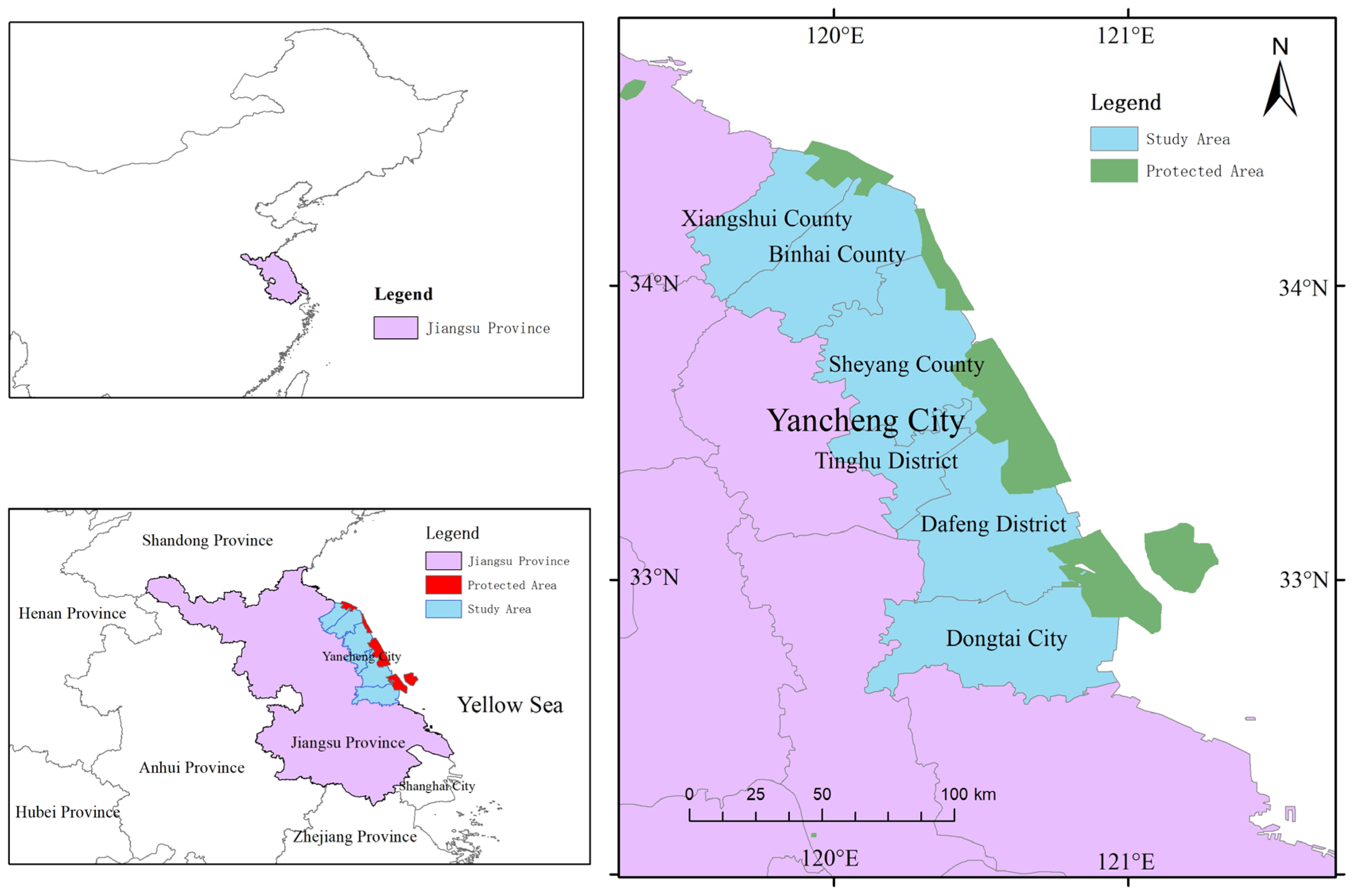
The Yancheng Wetland National Nature Reserve for Rare Birds in Jiangsu Province is located in the coastal area of eastern Yancheng, Jiangsu Province, between 32°34′–34°28′ N latitude and 119°27′–121°16′ E longitude. It covers a total area of approximately 247,260 hectares with a coastline of about 582 km. As one of the world’s largest intertidal wetland systems, the reserve serves as a crucial wintering habitat for endangered species such as the red-crowned crane (Grus japonensis). It underwent two boundary adjustments in 2006 and 2011 and currently consists of five fragmented regions (see Figure 1). For this study, six administrative divisions within the reserve’s jurisdiction were selected as the research area, namely Binhai County, Dafeng District, Dongtai City, Sheyang County, Tinghu District, and Xiangshui County. The selection of administrative units as the analytical basis is justified by the following considerations: (1) wetland protection and management decisions, including land use planning and zoning regulations, are implemented at the administrative-unit level in China; (2) socioeconomic statistical data (e.g., GDP, population, fiscal revenue) are only available at the county (city, district) scale; and (3) wetlands account for more than 20% of the total area in each of the six administrative units, ensuring that the spatial analysis at this scale captures meaningful ecological variation. However, we acknowledge that administrative boundaries do not perfectly coincide with ecological boundaries (e.g., wetland habitat patches or bird migration corridors), and this limitation is addressed in Section 4.

2.2. Data Sources and Processing

(1) Land use data: Derived from the GLC_FCS30D (1985–2022, 30 m) global land cover dynamic monitoring product on the Zenodo platform. This product has been validated globally with an overall accuracy exceeding 80%, and its classification system (including wetland types such as tidal flats, aquaculture ponds, and salt marshes) is appropriate for distinguishing the major land cover types in the Yancheng coastal region. Two datasets (E115N35 and E120N35) were selected based on the latitude and longitude range of the study area. Land cover types from 2010 to 2022 were extracted, followed by data reading and preprocessing in ArcGIS 10.2 (Esri, Redlands, CA, USA). It should be noted that the GLC_FCS30D product provides land cover (i.e., the physical surface type), which is interpreted in this study as the spatial manifestation of land use activities (such as aquaculture, agriculture, and urban construction). While land cover and land use are conceptually distinct, the former serves as a reliable proxy for the latter in spatial pattern analysis.

(2) Climate and vegetation data: Annual average temperature, annual precipitation, and Normalized Difference Vegetation Index (NDVI) were obtained from the 1 km resolution raster dataset of China on the Earth Resource Data Cloud platform (www.gis5g.com). To ensure spatial compatibility with the 30 m land cover data, the 1 km climate and NDVI rasters were resampled to 30 m resolution using the bilinear interpolation method in ArcGIS 10.2, with the WGS 1984 UTM Zone 51N projection maintained as the consistent spatial reference framework.

(3) Socioeconomic data: To comprehensively capture the multifaceted influences of socioeconomic development on landscape fragmentation, 17 variables were selected across the economic, social, and ecological systems.

For the economic system, GDP and industrial added values reflect economic scale and structure, which drive land conversion through industrial expansion and infrastructure construction. Fiscal revenue and expenditure indicate the capacity for ecological investment. Income and consumption variables reflect welfare levels and associated demand for construction land. Port throughput and industrial output capture external trade and manufacturing intensity, closely linked to coastal land occupation and transport corridor expansion.

For the social system, population density directly indicates human activity pressure on natural landscapes. Crop area and output reflect agricultural intensity—a key driver of wetland conversion to farmland and patch dissection. Aquatic product output captures aquaculture intensity, where high-density pond layouts create spatial barriers that impede connectivity. The number of books in public libraries and health technical personnel reflects regional cultural, educational, and healthcare development levels. Regions with higher development levels tend to have better-educated populations and stronger environmental awareness, which may indirectly support conservation-oriented land-use decisions. Additionally, the spatial distribution of public service facilities contributes to built-up area expansion, indirectly influencing landscape configuration.

For the ecological system, temperature and precipitation influence the hydrological regime and vegetation growth in coastal wetlands, affecting habitat quality and wetland boundary stability. NDVI serves as an indicator of vegetation cover and productivity, reflecting the overall ecological condition.

Statistical years range from 2011 to 2022, and all socioeconomic data were obtained from the Yancheng Statistical Yearbook and the Jiangsu Statistical Yearbook, with missing values interpolated using linear methods.

(4) Data processing: ArcGIS was used for raster-administrative region matching and zonal statistics; mean/area-weighted mean aggregation was adopted at the county (city, district) and township scales. Land use was uniformly classified into six categories: wetland, cultivated land, construction land, forest land, water body, and unused land. Classification accuracy was evaluated using a confusion matrix, with an overall accuracy and Kappa coefficient of no less than 85% and 0.80, respectively.

2.3. Research Methods

2.3.1. Landscape Pattern Indices and Fragmentation Index System

To characterize the comprehensive characteristics of landscape fragmentation in terms of “quantity-shape-structure-diversity”, four typical indices were selected [18,19,20,21,22] (see

Table 1. Landscape pattern index.

Landscape Pattern Index	Symbol	Calculation Formula	Meaning
Patch Density	PD	PD = ${\displaystyle \frac{{\mathrm{N}}_{\mathrm{i}}}{\mathrm{A}}}$, where A is the total landscape area in the study area, and ${\mathrm{N}}_{\mathrm{i}}$ is the number of patches of the i-th landscape element.	Represents the total number of patches per unit area.
Edge Density	ED	ED = ${\displaystyle \frac{{\displaystyle {\sum }_{\mathrm{i}=1}^{\mathrm{M}}}{\displaystyle {\sum }_{\mathrm{j}=1}^{\mathrm{M}}}{\mathrm{P}}_{\mathrm{ij}}}{\mathrm{A}}}$, where ${\mathrm{P}}_{\mathrm{ij}}$ is the boundary length between the i-th and j-th landscape element patches in the landscape.	Indicates the degree of landscape fragmentation: the larger the value, the higher the degree of landscape division and fragmentation.
Landscape Division	DIVISION	$\mathrm{DIVISION} = 1-{\displaystyle {\sum }_{\mathrm{j}=1}^{\mathrm{n}}}{\left({\displaystyle \frac{{\mathrm{a}}_{\mathrm{j}}}{\mathrm{A}}}\right)}^2$, where ${\mathrm{a}}_{\mathrm{j}}$ is the area of the j-th patch in the landscape.	The larger the index, the more fragmented the patches within the landscape type, and the more complex the landscape.
Shannon’s Diversity Index	SHDI	SHDI = $-{\displaystyle {\sum }_{\mathrm{j}=1}^{\mathrm{n}}}\left({\mathrm{P}}_{\mathrm{i}}\ln {\mathrm{P}}_{\mathrm{i}}\right)$, where ${\mathrm{P}}_{\mathrm{i}}$ is the proportion of the i-th landscape type to the total landscape area, and n is the number of landscape types.	Reflects landscape heterogeneity and is more sensitive to the uneven distribution of patch types in the landscape.

). These indices were selected based on their widespread use in landscape ecology and their complementary representation of different dimensions of fragmentation: PD captures the density of patch subdivision, ED reflects boundary complexity, DIVISION measures the degree of patch area dispersion, and SHDI characterizes landscape heterogeneity.

The study area was divided into six county-level administrative divisions, namely Binhai County, Dafeng District, Dongtai City, Sheyang County, Tinghu District, and Xiangshui County. The research period was divided into five phases: 2010, 2013, 2016, 2019, and 2022. The four indices listed in the above table were normalized first. Subsequently, the Cov-AHP method was applied to calculate the comprehensive landscape fragmentation index: the weights of the four indices were determined via Cov-AHP and then assigned to the normalized data to obtain the final comprehensive fragmentation index.

2.3.2. Cov-AHP

The judgment matrix of the traditional Analytic Hierarchy Process (AHP) relies entirely on expert scoring, leading to strong subjectivity. Furthermore, when there is a high correlation between indicators, it is prone to causing information redundancy. In contrast, the Covariance–Analytic Hierarchy Process (Cov-AHP) is optimized based on the framework of traditional AHP. It introduces covariance information between indicators and constructs the judgment matrix through the covariance matrix of sample data, which can truly reflect the collaborative variation relationship of each indicator in the actual data. While retaining the core advantage of the hierarchical structure of AHP, this method effectively reduces the bias caused by subjective weighting in the traditional method and mitigates the impact of information redundancy between indicators [23,24]. Before applying Cov-AHP, we conducted an exploratory correlation analysis among PD, ED, DIVISION, and SHDI. The Pearson correlation coefficients ranged from 0.62 to 0.89 (all p < 0.01), and Bartlett’s test of sphericity was significant (χ² = 156.3, df = 6, p < 0.001), confirming the presence of a significant covariance structure among the four metrics. This provides the empirical basis for using covariance-based weighting in Cov-AHP. The steps are as follows.

(1) Covariance and standardized matrix

Establish the full $\mathrm{p}$-dimensional index data covariance matrix $\mathrm{A}={\left({\mathrm{a}}_{\mathrm{i}\mathrm{j}}\right)}_{\mathrm{p}\times \mathrm{p}}$. Perform standardization processing, i.e., ${\mathrm{b}}_{\mathrm{i}\mathrm{j}}={\mathrm{a}}_{\mathrm{i}\mathrm{j}}/{\mathrm{a}}_{\mathrm{i}\mathrm{i}}$, to obtain the standardized covariance matrix $\mathrm{B}={\left({\mathrm{b}}_{\mathrm{i}\mathrm{j}}\right)}_{\mathrm{p}\times \mathrm{p}}$.

(2) Construction of the judgment matrix

Transform the standardized covariance matrix B to obtain the judgment matrix $\mathrm{C}={\left({\mathrm{c}}_{\mathrm{i}\mathrm{j}}\right)}_{\mathrm{p}\times \mathrm{p}}$:

$${\mathrm{c}}_{\mathrm{i}\mathrm{j}}={\mathrm{b}}_{\mathrm{i}\mathrm{j}}/\sqrt{{\mathrm{b}}_{\mathrm{i}\mathrm{j}}\times {\mathrm{b}}_{\mathrm{j}\mathrm{i}}}$$

(1)

(3) Weight recalculation

Obtain the weight vector $\mathsf{\omega }={({{\mathsf{\omega }}^{\prime }}_1, {{\mathsf{\omega }}^{\prime }}_2, {{\mathsf{\omega }}^{\prime }}_3, \dots , {\mathsf{\omega }\prime }_{\mathrm{p}})}^{\mathrm{T}}$ using the geometric mean method and the eigenvector method:

$${\mathrm{M}}_{\mathrm{i}}={\displaystyle {\prod }_{\mathrm{j}=1}^{\mathrm{p}}}{\mathrm{c}}_{\mathrm{i}\mathrm{j}}(\mathrm{i}=\mathrm{1,2},\dots ,\mathrm{p}), {\mathsf{\omega }}_{\mathrm{i}}=\sqrt[\mathrm{p}]{{\mathrm{M}}_{\mathrm{i}}}, {\mathsf{\omega }\prime }_{\mathrm{i}}={\displaystyle \frac{{\mathsf{\omega }}_{\mathrm{i}}}{{\sum }_{\mathrm{j}=1}^{\mathrm{p}}{\mathsf{\omega }}_{\mathrm{i}}}}$$

(2)

(4) Consistency test

Calculate the maximum eigenvalue ${\mathsf{\lambda }}_{\mathrm{m}\mathrm{a}\mathrm{x}}$ of matrix C:

$${\mathsf{\lambda }}_{\mathrm{m}\mathrm{a}\mathrm{x}}={\displaystyle \frac{1}{\mathrm{p}}}{\displaystyle {\sum }_{\mathrm{i}=1}^{\mathrm{p}}}{\displaystyle \frac{{\left(\mathrm{C}\mathrm{W}\right)}_{\mathrm{i}}}{{{\mathsf{\omega }}^{\prime }}_{\mathrm{i}}}}$$

(3)

Then derive the consistency index CI and consistency ratio CR:

$$\mathrm{C}\mathrm{I}={\displaystyle \frac{{\mathsf{\lambda }}_{\mathrm{m}\mathrm{a}\mathrm{x}}-\mathrm{p}}{\mathrm{p}-1}}$$

(4)

$$\mathrm{C}\mathrm{R}={\displaystyle \frac{\mathrm{C}\mathrm{I}}{\mathrm{R}\mathrm{I}}}$$

(5)

where RI is the random consistency index (see

Table 2. Random consistency standard comparison table.

p	1	2	3	4	5	6	7	8	9	10	11	12	…
RI	0.00	0.00	0.58	0.90	1.12	1.24	1.32	1.41	1.45	1.49	1.52	1.54	…

). When CR < 0.1, matrix C is generally considered to satisfy the consistency test. The obtained CR values for all periods were below 0.08, indicating that the weight structure is statistically distinguishable from a random structure.

(5) Comprehensive Fragmentation Index

Calculate the comprehensive fragmentation index for each region:

$${\mathrm{S}}_{\mathrm{j}}={\displaystyle {\sum }_{\mathrm{i}=1}^{\mathrm{p}}}{\mathsf{\omega }}_{\mathrm{i}\mathrm{j}}{\mathrm{t}}_{\mathrm{i}}\mathrm{j}=1, 2, \dots , \mathrm{n}$$

(6)

where ${\mathsf{\omega }}_{\mathrm{i}\mathrm{j}}$ is the weight corresponding to the $\mathrm{j}$-th indicator in the $\mathrm{p}$-indicator system, and ${\mathrm{t}}_{\mathrm{i}}$ is the value of the $\mathrm{p}$-th indicator for the $\mathrm{j}$-th region. A larger ${\mathrm{S}}_{\mathrm{j}}$ indicates a higher degree of fragmentation.

2.3.3. Generalized Additive Model (GAM) and Variable Selection

To identify the overall nonlinear relationships and interaction effects between fragmentation and driving factors [25], a GAM is constructed:

$$\mathrm{g}(\mathrm{u})={\mathrm{s}}_0+{\mathrm{s}}_1\left({\mathrm{X}}_1\right)+{\mathrm{s}}_2\left({\mathrm{X}}_2\right)+\cdots +{\mathrm{s}}_{\mathrm{p}}\left({\mathrm{X}}_{\mathrm{p}}\right)$$

(7)

$$\mathrm{u}=\mathrm{E}\left(\mathrm{Y}\right|{\mathrm{X}}_1,{\mathrm{X}}_2\dots {\mathrm{X}}_{\mathrm{p}})$$

(8)

where $\mathrm{g}\left(\mathrm{u}\right)$ is the link function, and ${\mathrm{s}}_{\mathrm{i}}\left({\mathrm{X}}_{\mathrm{i}}\right)$ is a smoothing function (a smooth spline function is used in this study). Given the continuous distribution of the LFI response variable, a Gaussian distribution with an identity link function was adopted for the GAMs. The optimal smoothness of each smoothing term was selected using the Generalized Cross-Validation (GCV) criterion, with the maximum degrees of freedom constrained to k = 4 for univariate models and k = 10 for interaction terms to balance model flexibility against overfitting [25].

For the multivariate GAMs, we adopted a stepwise model-building strategy to avoid overfitting given the limited sample size (n = 6 counties × 5 time periods = 30 observations for the county-level analysis). The univariate GAM analysis serves as an exploratory tool to identify the functional form (linear vs. nonlinear) of each variable’s relationship with LFI, rather than as a predictive model. Variables with edf > 1 and p < 0.05 in univariate models were retained as candidate variables for multivariate models. The multivariate model complexity was controlled by monitoring the Akaike Information Criterion (AIC) and the proportion of deviance explained, with the final model selected as the one achieving the lowest AIC value [25].

The estimation of the smoothing function ${\mathrm{s}}_{\mathrm{i}}\left({\mathrm{X}}_{\mathrm{i}}\right)$ for each variable uses the penalized least squares method. The penalized sum of squares is

$${\mathrm{S}}_{\mathrm{W}}({\mathrm{s}}_1,\dots ,{\mathrm{s}}_{\mathrm{m}})={{\displaystyle {\sum }_{\mathrm{i}}^{\mathrm{m}}}{\mathrm{w}}_{\mathrm{i}}({\mathsf{\eta }}_{\mathrm{i}}-{\displaystyle {\sum }_{\mathrm{i}=1}^{\mathrm{m}}}{\mathrm{s}}_{\mathrm{j}}\left({\mathrm{x}}_{\mathrm{i}\mathrm{j}}\right))}^2+{\displaystyle {\sum }_{\mathrm{j}=1}^{\mathrm{m}}}{\mathsf{\lambda }}_{\mathrm{j}}\int {{\mathrm{s}}_{\mathrm{j}}}^{″}{\left(\mathrm{x}\right)}^2\mathrm{d}\mathrm{x}$$

(9)

where $\int {{\mathrm{s}}_{\mathrm{j}}}^{″}{\left(\mathrm{x}\right)}^2\mathrm{d}\mathrm{x}$ is the smoothness penalty term. The penalized least squares combined with the backfitting algorithm is used for iterative estimation.

Taking the comprehensive index of landscape fragmentation as the response variable, explanatory variables were selected from the Economic–Ecological–Social (EES) system (see

Table 3. Influencing factors of landscape fragmentation.

System	Variable Name	Meaning	Unit
Economic System	x1	Regional Gross Domestic Product	100 million yuan
	x2	Added Value of Primary Industry	100 million yuan
	x3	Added Value of Secondary Industry	100 million yuan
	x4	Added Value of Tertiary Industry	100 million yuan
	x5	General Public Budget Revenue	10 million yuan
	x6	General Public Budget Expenditure	10 million yuan
	x7	Total Retail Sales of Consumer Goods	100 million yuan
	x8	Per Capita Disposable Income	1000 yuan
	x9	Per Capita Living Consumption Expenditure	1000 yuan
	x10	Port Throughput	10,000 tons
	x11	Industrial Gross Output Value Index	%
Social System	x12	Population Density	persons per square kilometer
	x13	Aquatic Product Output	10,000 tons
	x14	Crop Sown Area	1000 hectares
	x15	Total Crop Output	10,000 tons
	x16	Public Library Collections	1000 volumes
	x17	Number of Health Technical Personnel	100 persons
Ecosystem	x18	Annual Average Temperature	°C
	x19	Annual Average Precipitation	millimeters
	x20	Normalized Difference Vegetation Index (NDVI)	%

) to establish a model for exploring the influencing factors of landscape fragmentation. For the economic system, Gross Regional Product (GRP)—which measures economic status and is associated with conservation investment and residents’ awareness—added value of the primary, secondary, and tertiary industries (as different industries exert distinct impacts on habitats, such as agricultural activities altering land use and industrial production causing pollution), government budget revenue and expenditure (reflecting ecological conservation investment and resource utilization efficiency), residents’ income and expenditure as well as total retail sales of consumer goods (indicating living standards and correlating with environmental awareness), and port throughput and total industrial output value index (reflecting the intensity of economic activities and affecting the ecological environment) were chosen; for the ecological system, annual average precipitation and temperature (directly influencing the breeding and migration of red-crowned cranes) and Normalized Difference Vegetation Index (NDVI, a metric for vegetation condition and an indicator of habitat quality) were selected; for the social system, population density (reflecting the pressure of human activities), output of agriculture and fishery-related products (indicating the intensity of agricultural and fishery activities that impact habitats and food sources), and the number of books in libraries and health workers (reflecting the level of cultural, educational, and medical development, which is associated with environmental awareness and habitat protection) were included.

2.3.4. Geographically Weighted Regression (GWR)

To test the spatial non-stationarity of the effects of driving factors [26,27], a GWR is constructed at the sampling point $\left({\mathrm{u}}_{\mathrm{i}},{\mathrm{v}}_{\mathrm{i}}\right)$:

$${\mathrm{y}}_{\mathrm{i}}={\mathsf{\beta }}_0\left({\mathrm{u}}_{\mathrm{i}},{\mathrm{v}}_{\mathrm{i}}\right)+{\sum }_{\mathrm{k}}{\mathsf{\beta }}_{\mathrm{k}}{\left({\mathrm{u}}_{\mathrm{i}},{\mathrm{v}}_{\mathrm{i}}\right)\mathrm{x}}_{\mathrm{i}\mathrm{k}}+{\mathsf{\epsilon }}_{\mathrm{i}}$$

(10)

In contrast to the global OLS [28]:

$${\mathrm{y}}_{\mathrm{i}}={\mathsf{\beta }}_0+{\sum }_{\mathrm{k}}{\mathsf{\beta }}_{\mathrm{k}}{\mathrm{x}}_{\mathrm{i}\mathrm{k}}+{\mathsf{\epsilon }}_{\mathrm{i}}$$

(11)

GWR adopts an adaptive bi-square kernel function, and the bandwidth is optimized via AICc. The spatial distribution of regression coefficients ${\mathsf{\beta }}_{\mathrm{k}}$ is used to identify dominant driving factors and their spatial heterogeneity [29]. The spatial units for GWR analysis were 30 m × 30 m grid cells. For each grid cell, the corresponding LFI value and driver variable values were extracted. Local regression coefficients were estimated using the coordinates of each grid cell centroid for the spatial weight matrix calculation. The township-scale aggregation was applied for the final presentation of results to balance computational feasibility with interpretability at a meaningful management scale.

The estimation of GWR parameters is:

$$\widehat{\mathsf{\beta }}\left({\mathrm{u}}_{\mathrm{i}},{\mathrm{v}}_{\mathrm{i}}\right)={\left({\mathrm{X}}^{\mathrm{T}}\mathrm{W}\left({\mathrm{u}}_{\mathrm{i}},{\mathrm{v}}_{\mathrm{i}}\right)\mathrm{X}\right)}^{-1}{\mathrm{X}}^{\mathrm{T}}\mathrm{W}\left({\mathrm{u}}_{\mathrm{i}},{\mathrm{v}}_{\mathrm{i}}\right)\mathrm{Y}$$

(12)

Herein,

$$\mathrm{X}=\left[\begin{array}{ccc}1& \cdots & {\mathrm{x}}_{1\mathrm{k}}\\ ⋮& \ddots & ⋮\\ 1& \cdots & {\mathrm{x}}_{\mathrm{n}\mathrm{k}}\end{array}\right]$$

(13)

$$\mathrm{W}\left({\mathrm{u}}_{\mathrm{i}},{\mathrm{v}}_{\mathrm{i}}\right)=\mathrm{W}\left(\mathrm{i}\right)\left[\begin{array}{ccc}{\mathrm{w}}_{\mathrm{i}1}& \cdots & 0\\ ⋮& \ddots & ⋮\\ 0& \cdots & {\mathrm{w}}_{\mathrm{i}\mathrm{n}}\end{array}\right]$$

(14)

$$\mathsf{\beta }=\left[\begin{array}{ccc}{\mathsf{\beta }}_0\left({\mathrm{u}}_1,{\mathrm{v}}_1\right)& \cdots & {\mathsf{\beta }}_{\mathrm{k}}\left({\mathrm{u}}_1,{\mathrm{v}}_1\right)\\ ⋮& \ddots & ⋮\\ {\mathsf{\beta }}_{\mathrm{n}}\left({\mathrm{u}}_{\mathrm{n}},{\mathrm{v}}_{\mathrm{n}}\right)& \cdots & {\mathsf{\beta }}_{\mathrm{k}}\left({\mathrm{u}}_{\mathrm{n}},{\mathrm{v}}_{\mathrm{n}}\right)\end{array}\right]$$

(15)

3. Results

3.1. Comprehensive Fragmentation Index and Dynamics of Yancheng Coastal Wetlands

The comprehensive landscape fragmentation index (LFI) of the six counties (cities, districts) in the study area for the years 2010, 2013, 2016, 2019, and 2022 is presented in

Table 4. Comprehensive index of landscape fragmentation by county and region from 2010 to 2022.

Year	2010	2013	2016	2019	2022
Binhai	0.1857	0.2040	0.2106	0.2809	0.2409
Dafeng	0.6027	0.6699	0.7498	0.7101	0.6976
Dongtai	0.2787	0.3112	0.4027	0.3673	0.3798
Sheyang	0.5612	0.5587	0.4129	0.5580	0.5700
Tinghu	0.2729	0.3248	0.4129	0.5836	0.6084
Xiangshui	0.6290	0.6537	0.6622	0.7220	0.7358

. Overall, the regional landscape fragmentation level has shown a slow upward trend, with significant differences among counties. The LFI values range from 0 (least fragmented) to 1 (most fragmented), and the index integrates four dimensions: patch density (PD), edge density (ED), landscape division (DIVISION), and Shannon’s diversity index (SHDI), weighted using the Cov-AHP method. Higher LFI values indicate a greater number of patches, higher boundary complexity, more dispersed patch areas, and greater landscape diversity, collectively reflecting a higher degree of landscape fragmentation.

(1) County-level LFI Comparison (2022)

In 2022, the LFI (Comprehensive Landscape Fragmentation Index) of the study area in descending order was: Xiangshui > Dafeng > Tinghu > Sheyang > Dongtai > Binhai. The landscape fragmentation level in northern and central regions with high development intensity was significantly higher than that in Dongtai and Binhai, showing obvious spatial differentiation.

(2) Temporal Evolution (2010–2022)

Xiangshui County: LFI continued to rise, indicating a stable increase trend.

Dafeng District: LFI first increased and then decreased slightly, remaining at a high level after peaking in 2016.

Tinghu District: LFI recorded the largest increase (+0.336), rising rapidly from a low level to a medium-high level.

Sheyang County: LFI dropped significantly in 2016 and then recovered, with the smallest net increase (approximately +0.009).

Dongtai City: LFI showed a “rise—decline—slight recovery” trend.

Binhai County: LFI fluctuated and rose at a low overall level, reaching a relative high in 2019 before declining slightly.

(3) Ecological Implications

An increase in LFI indicates a rise in the number of patches and boundary complexity, along with a decrease in aggregation and connectivity. The continuous or rapid increase in LFI in Xiangshui, Dafeng, and Tinghu suggests enhanced ecological vulnerability and increased conservation pressure. Although Dongtai and Binhai maintained a relatively low overall LFI level, their phased increases indicate potential local disturbance risks. The above patterns are closely related to the expansion of construction land, industrial layout, and changes in vegetation conditions. In subsequent research, zonal management and targeted ecological restoration should be carried out in combination with driving mechanism analysis.

3.2. Analysis of the Impact of the EES System on Landscape Fragmentation Based on GAM

3.2.1. Analysis of Influencing Factors of Landscape Fragmentation Based on Univariate GAM

Univariate Generalized Additive Models (GAMs) were constructed for 11 economic factors, 6 social factors, and 3 ecological factors respectively, with the results presented in

Table 5. Fitting effect of univariate GAM.

Smoothing Term	Variable Meaning	Estimated Degrees of Freedom	Reference Degrees of Freedom	F	P	Adjusted R-Squared	Variance Explained
s(x12)	Population Density	7.988	8.712	32.91	<2 × 10−16 ***	0.787	80.90%
s(x14)	Crop Sown Area	7.843	8.592	22.07	<2 × 10−16 ***	0.712	74.10%
s(x13)	Aquatic Product Output	6.909	7.939	16.79	<2 × 10−16 ***	0.634	66.70%
s(x15)	Total Crop Output	5.01	6.044	8.46	<2 × 10−6 ***	0.396	43.60%
s(x20)	NDVI	1	1	12.27	<2 × 10−4 ***	0.128	13.90%
s(x17)	Number of Health Technical Personnel	2.664	3.321	2.736	0.0476 **	0.095	12.60%
s(x10)	Port Throughput	1	1	8.685	0.00426 ***	0.0908	10.30%
s(x16)	Public Library Collections	1	1	4.227	0.0432 **	0.0402	5.27%
s(x18)	Annual Average Temperature	1	1	3.466	0.0665 *	0.031	4.36%
s(x8)	Per Capita Disposable Income	1	1	2.902	0.0926 *	0.0241	3.68%
s(x11)	Industrial Gross Output Value Index	1.794	2.28	0.819	0.461	0.0115	3.46%
s(x19)	Annual Average Precipitation	1.575	1.939	0.577	0.506	0.0054	2.57%
s(x5)	General Public Budget Revenue	1.564	1.935	0.729	0.540	0.0049	2.51%
s(x9)	Per Capita Living Consumption Expenditure	1	1	1.642	0.204	0.0083	2.12%
s(x4)	Added Value of Tertiary Industry	1	1	1.081	0.302	0.00105	1.40%
s(x1)	Regional Gross Domestic Product	1	1	0.848	0.360	−0.0020	1.10%
s(x2)	Added Value of Primary Industry	1	1	0.62	0.433	−0.0050	0.81%
s(x3)	Added Value of Secondary Industry	1	1	0.432	0.513	−0.0074	0.57%
s(x6)	General Public Budget Expenditure	1	1	0.424	0.517	−0.0075	0.56%
s(x7)	Total Retail Sales of Consumer Goods	1	1	0.016	0.900	−0.0129	0.02%

Notes: * p < 0.1, ** p < 0.05, *** p < 0.01. Same for the following tables.

. Overall, the social system exhibited the highest explanatory power, followed by the ecological system, while the economic system showed relatively weak overall explanatory power; the effective degrees of freedom (edf) of the smooth terms for most key variables were greater than 1, indicating significant nonlinear relationships. The univariate GAM analysis was based on n = 30 observations (6 counties × 5 time periods). Variables with edf > 1 and p < 0.05 were identified as having significant nonlinear relationships with LFI and were retained for multivariate model development.

(1) Ranking of Explanatory Power and Significance

At the univariate level, the “human-agricultural” variables in the social system exhibited the strongest explanatory power: population density showed the most stable and robust response to landscape fragmentation, followed by sown area and aquatic product output related to agricultural intensity; among ecological state variables, NDVI displayed a clear signal but moderate explanatory strength. The effective degrees of freedom (edf) of the smooth terms for these key variables were all greater than 1, indicating the presence of nonlinear/threshold effects—linear assumptions are insufficient to characterize their impacts. In contrast, the remaining variables demonstrated higher uncertainty in univariate models and failed to provide robust individual explanations.

(2) Relative Roles of Ecological and Social Factors

The overall pattern presented as “social activity-driven and ecological condition-regulated”: social factors (especially population density and agricultural production) directly alter land use and patch patterns, serving as the primary driver of intensified fragmentation; ecological factors (NDVI, temperature, precipitation) functioned as buffers/threshold regulators—when vegetation conditions are favorable, the rate of fragmentation increase is significantly constrained. However, climate factors alone exert limited direct effects and are more likely to act indirectly by influencing vegetation and hydrological processes.

(3) Relatively Weak Explanatory Power of Economic Factors

Macroeconomic indicators such as GDP, industrial added value, and fiscal revenue/expenditure showed weak signals in univariate models. This does not imply irrelevance but rather suggests three plausible explanations: structural collinearity with social/ecological variables (e.g., economic scale is highly correlated with population density and construction intensity), making it difficult to distinguish individual effects in single-variable modeling; mismatched scales and time lags (county-level annual economic data often affect landscape patterns through years of accumulation and policy implementation); greater suitability as linear control variables or for revealing action pathways through interactions/nonlinear terms in multivariate models.

(4) Methodological Implications

Key variables (x12, x14, x13, x15, x20) exhibited edf > 1 and p < 0.001, confirming the existence of nonlinear effects between these factors and landscape fragmentation. This provides a methodological basis for introducing interaction terms in subsequent multivariate GAMs and testing spatial nonstationarity in Geographically Weighted Regression (GWR). For economic variables with low explanatory power but theoretical importance, they can be incorporated as linear control variables in multivariate models.

3.2.2. Analysis of Influencing Factors of Landscape Fragmentation Based on Optimized GAMs

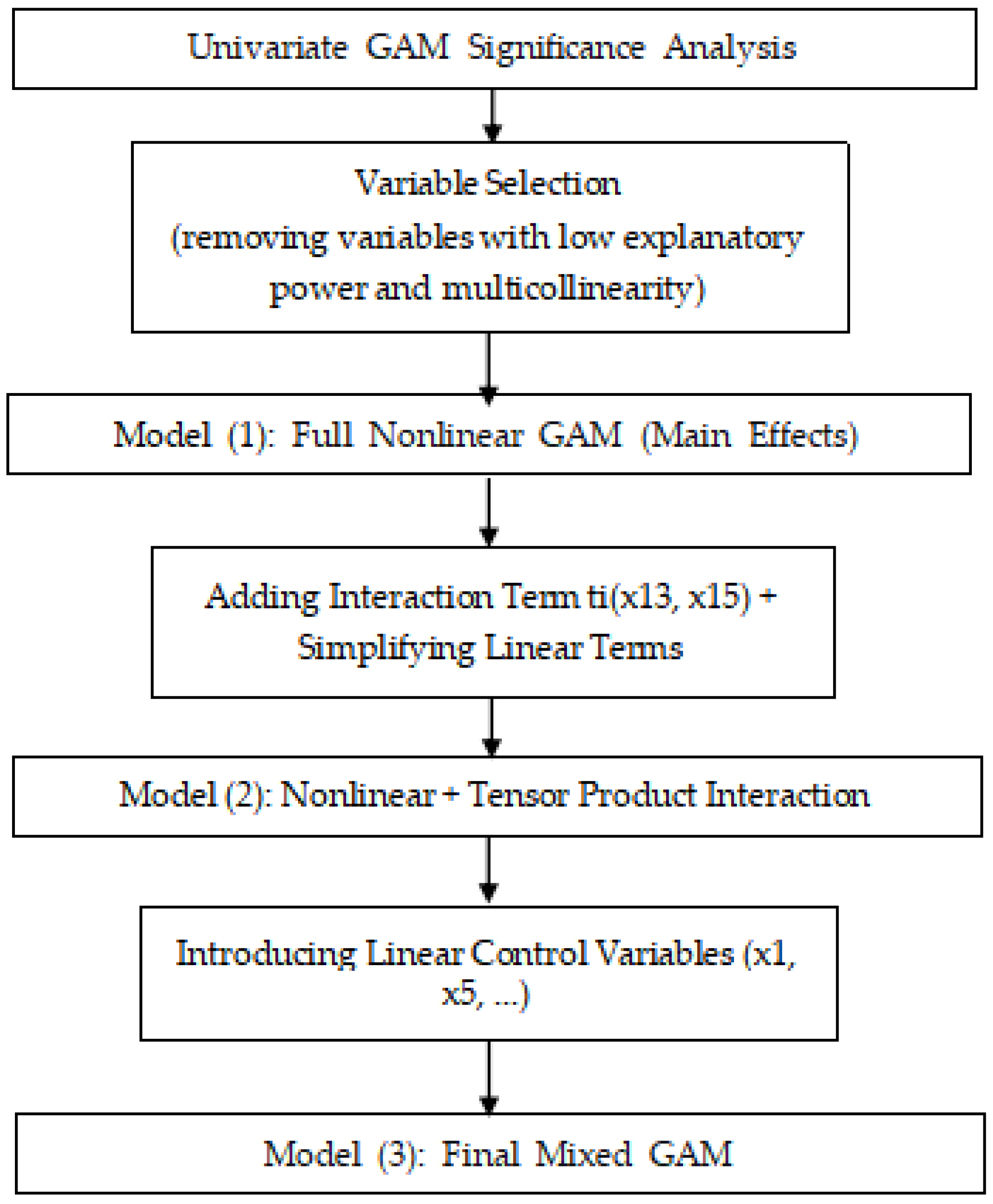
To improve the interpretability and robustness of the model, a stepwise optimization strategy is adopted to construct three types of GAMs (see Figure 2).

Model (1): Taking 8 variables (including population density, agriculture and fishery intensity, social public services, precipitation, and NDVI) as nonlinear predictors:

$$\log \left(\mathrm{y}\right) = \mathsf{\beta } + \mathrm{s}\left(\mathrm{x}12\right) + \mathrm{s}\left(\mathrm{x}13\right) + \mathrm{s}\left(\mathrm{x}14\right) + \mathrm{s}\left(\mathrm{x}15\right) + \mathrm{s}\left(\mathrm{x}16\right) + \mathrm{s}\left(\mathrm{x}17\right) + \mathrm{s}\left(\mathrm{x}19\right) + \mathrm{s}\left(\mathrm{x}20\right) + \mathsf{\epsilon }$$

(16)

where β is the intercept term, s(x) represents the nonlinearity of variable x, and $\mathsf{\epsilon }$ is the random error term.

Model (2): On the basis of the baseline model, the interaction term ti(x13, x15) (Aquatic Product Output × Total Crop Output) is incorporated, and variables with approximate linearity are reduced to linear terms to simplify the structure.

$$\log \left(\mathrm{y}\right)=\mathsf{\beta }+\mathrm{s}\left(\mathrm{x}12\right)+\mathrm{s}\left(\mathrm{x}13\right)+\mathrm{s}\left(\mathrm{x}14\right)+\mathrm{s}\left(\mathrm{x}15\right)+\mathrm{s}\left(\mathrm{x}19\right)+\mathrm{s}\left(\mathrm{x}20\right)+\mathrm{ti}(\mathrm{x}13,\mathrm{x}15)+\mathsf{\epsilon }$$

(17)

where β is the intercept term, s(x) represents the nonlinearity of variable x, ti(x13,x15) denotes the interaction term of x13 and x15, and $\mathsf{\epsilon }$ is the random error term.

Model (3): On the basis of Model (2), linear control variables (such as GDP, general public budget revenue, per capita consumption expenditure, and industrial gross output value index) are further introduced, forming a comprehensive model of “nonlinear main effect + key interaction + linear control”.

$$\log \left(\mathrm{y}\right)=\mathsf{\beta }+\mathrm{s}\left(\mathrm{x}12\right)+\mathrm{s}\left(\mathrm{x}14\right)+\mathrm{s}\left(\mathrm{x}15\right)+\mathrm{s}\left(\mathrm{x}19\right)+\mathrm{s}\left(\mathrm{x}20\right)+\mathrm{ti}(\mathrm{x}13,\mathrm{x}15)+\mathsf{\beta }1\mathrm{x}1+\mathsf{\beta }2\mathrm{x}5+\mathsf{\beta }3\mathrm{x}9+\mathsf{\beta }4\mathrm{x}11+\mathsf{\beta }5\mathrm{x}13+\mathsf{\epsilon }$$

(18)

where β is the intercept term, s(x) represents the nonlinearity of variable x, ti(x13,x15) denotes the interaction term of x13 and x15, βx are linear terms, and $\mathsf{\epsilon }$ is the random error term.

(1) Nonlinear Main Effects: Human–Agriculture–Vegetation as Core Drivers

In the final model, the smooth terms of population density, crop sown area, total crop output, annual precipitation, and NDVI were all significant (see

Table 6. The fitting effect of multivariable GAMs (three).

Smoothing Term	Estimated Degrees of Freedom	Reference Degrees of Freedom	F	P
s(x12)	5.377	6.169	13.822	<2.00 × 10−16 ***
s(x14)	3.886	4.669	2.386	0.03858 **
s(x15)	5.424	6.159	2.436	0.02108 **
s(x19)	5.782	6.818	3.514	0.00447 ***
s(x20)	4.412	5.34	9.399	4.43 × 10−6 ***
ti(x13,x15)	6.898	7.962	3.748	0.00249 ***

), indicating that landscape fragmentation exhibits nonlinear/threshold responses to these variables. Mechanistically, population and agricultural production directly alter land use and patch configuration, serving as the primary drivers of intensified fragmentation; the ecological-climatic context reflected by NDVI and precipitation shows a regulatory/buffering association with fragmentation.

(2) Key Interaction: Synergistic Effects of Agricultural and Fishery Intensities

The interaction term ti(x13, x15) was significant (Table 6), suggesting that when fishery output and total agricultural output increase simultaneously, their combined impact on fragmentation is greater than the simple sum of their individual effects. This implies that the rise in integrated land–sea use intensity amplifies the risk of landscape fragmentation. Priority should be given to implementing coordinated total amount control of agricultural and fishery activities and constructing ecological buffer zones in the transitional areas where agricultural and fishery activities intersect.

(3) Linear Controls: Directional Effects of Economic Magnitude on Fragmentation

After controlling for nonlinear main effects and interactions, GDP, general public budget revenue, and total industrial output value index generally showed an inhibitory relationship with fragmentation, while per capita household consumption expenditure and aquatic product output (linear component) exhibited a promoting relationship (see

Table 7. Parameter estimation and hypothesis testing.

Variable	Estimate	Std. Error	t	P
(Intercept)	3.2015295	0.3035727	10.546	3.81 × 10−13 ***
x1	−0.0006618	0.0002585	−2.56	0.014341 **
x5	−0.0002318	0.0001067	−2.172	0.035772 **
x9	0.0264953	0.0101216	2.618	0.012417 **
x11	−0.0045224	0.000935	−4.837	1.97 × 10−5 ***
x13	0.0751327	0.0197398	3.806	0.000472 ***

). This indicates that economic scale itself does not inevitably lead to increased fragmentation; its direction depends on expenditure structure and industrial structure: when public finance and industrial efficiency improve, fragmentation pressure may be alleviated; conversely, consumption expansion and high-intensity fishery production may bring about collateral effects of intensified fragmentation.

(4) Model Goodness-of-Fit and Diagnosis

Compared with the models from the previous two steps, Model (III) achieved a better balance between goodness-of-fit and complexity (see Table 6 and Table 7), with residual spatial autocorrelation effectively controlled. It is therefore suitable for the subsequent interpretation of policy implications and spatial zonal management.

3.3. Analysis of the Impact of the EES System on Landscape Fragmentation Based on GWR

Considering the potential spatial heterogeneity in the effects of variables, this study constructed a Geographically Weighted Regression (GWR) model at the township scale to identify the spatial drivers of the Comprehensive Landscape Fragmentation Index (LFI) from the perspective of the Economic–Ecological–Social (EES) system. For the economic system, Gross Regional Product (GDP) was selected; for the ecological system, annual average temperature, annual average precipitation, and Normalized Difference Vegetation Index (NDVI) were chosen; and for the social system, population density was adopted.

3.3.1. Spatial Autocorrelation Analysis

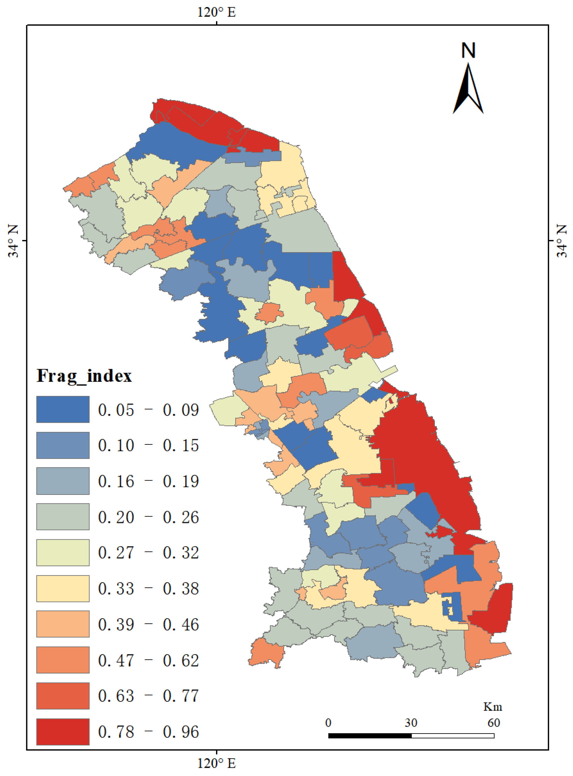
Spatial autocorrelation analysis was performed on the response variable LFI [30,31]: LFI exhibited significant positive spatial autocorrelation at the township scale (see Figure 3); statistical test results are presented in

Table 8. Global Moran I index test.

Moran I Index	Expected Index	Variance	z-Score	p-Value
0.143392	−0.009901	0.003928	2.445799	0.014453 **

, indicating that landscape fragmentation is spatially clustered rather than randomly distributed. This provides a prerequisite for conducting spatially varying coefficient modeling with GWR.

3.3.2. Kernel Function and Bandwidth Selection

Two types of kernel functions, Gaussian and bisquare, were compared, and the bandwidth was selected based on the dual criteria of AIC and Cross-Validation (CV). The results showed that the combination of Gaussian + CV achieved the optimal balance between goodness of fit and model stability (see

Table 9. Each kernel function, the optimal bandwidth under the criterion and the score.

Kernel Function	Gaussian		Bisquare
Criterion	AIC	CV	AIC	CV
Optimal Bandwidth	0.1916468	0.159589	0.5639261	0.5493058
AIC	774.6644	759.8082	784.7101	782.8595
R2	0.8460481	0.8757139	0.827708	0.8324985
Adjusted R2	0.7802629	0.7979014	0.7671751	0.770054

). On this basis, the kernel function and optimal bandwidth settings of subsequent models were determined.

3.3.3. GWR Model Construction and Overall Characteristics

Taking the Landscape Fragmentation Index (LFI) as the dependent variable and Gross Domestic Product (GDP), population density, annual average temperature, annual average precipitation, and Normalized Difference Vegetation Index (NDVI) as explanatory variables, a Geographically Weighted Regression (GWR) model was constructed and further compared with the global Ordinary Least Squares (OLS) model. Diagnostic results indicated that the GWR model improved the goodness of fit and effectively reduced the spatial autocorrelation of residuals, which demonstrated that the impacts of dominant driving factors on landscape fragmentation varied with spatial locations.

From the perspective of overall statistical characteristics (see

Table 10. GWR model regression coefficient descriptive statistics.

Name	Mean	Maximum	Minimum	Median	Standard Deviation	Range
Regional Gross Domestic Product	1.5012	30.8934	−4.0078	−0.2165	5.9963	34.9012
NDVI	−0.9152	−0.1189	−2.5245	−1.0453	0.5244	2.4057
Population Density	−0.8772	1.7385	−11.3852	−0.5041	1.9207	13.1237
Annual Average Precipitation	0.4152	5.4552	−0.3561	0.2020	0.8616	5.8113
Annual Average Temperature	0.3422	1.5865	−5.3448	0.5657	1.1407	6.9313

), GDP exerted the strongest impact, followed by NDVI and population density, while climatic factors showed relatively weak effects overall. Meanwhile, the coefficients of all variables presented significant spatial dispersion, which further verified the existence of spatial non-stationarity. Notably, the coefficients for GDP and population density range from negative to positive values (GDP: −4.01 to 30.89; population density: −11.39 to 1.74), indicating that the direction of influence of these factors varies across the study area. This suggests that the effects of these drivers are not uniformly positive or negative but rather depend on local contextual conditions.

3.3.4. GWR Model Analysis

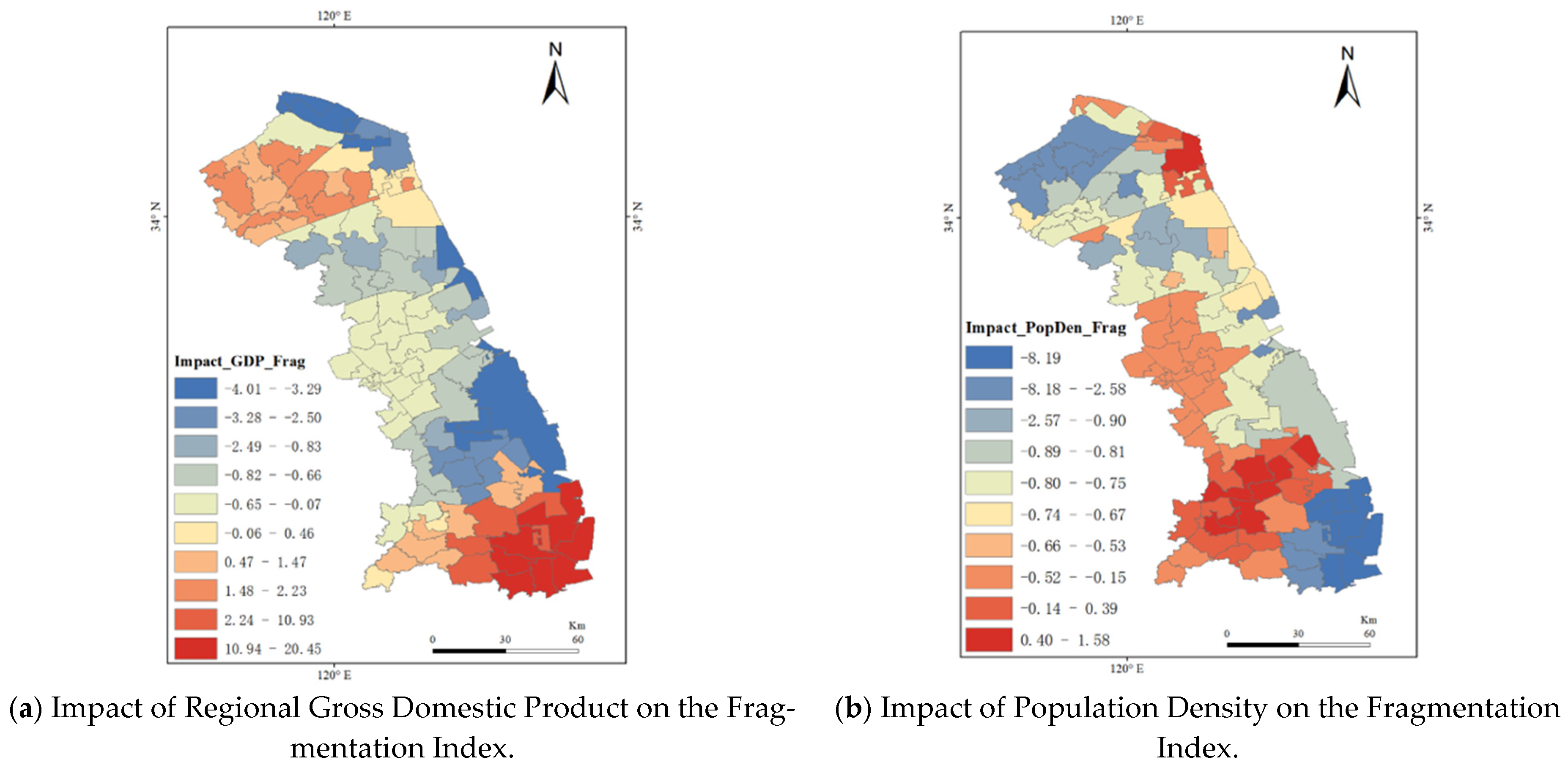
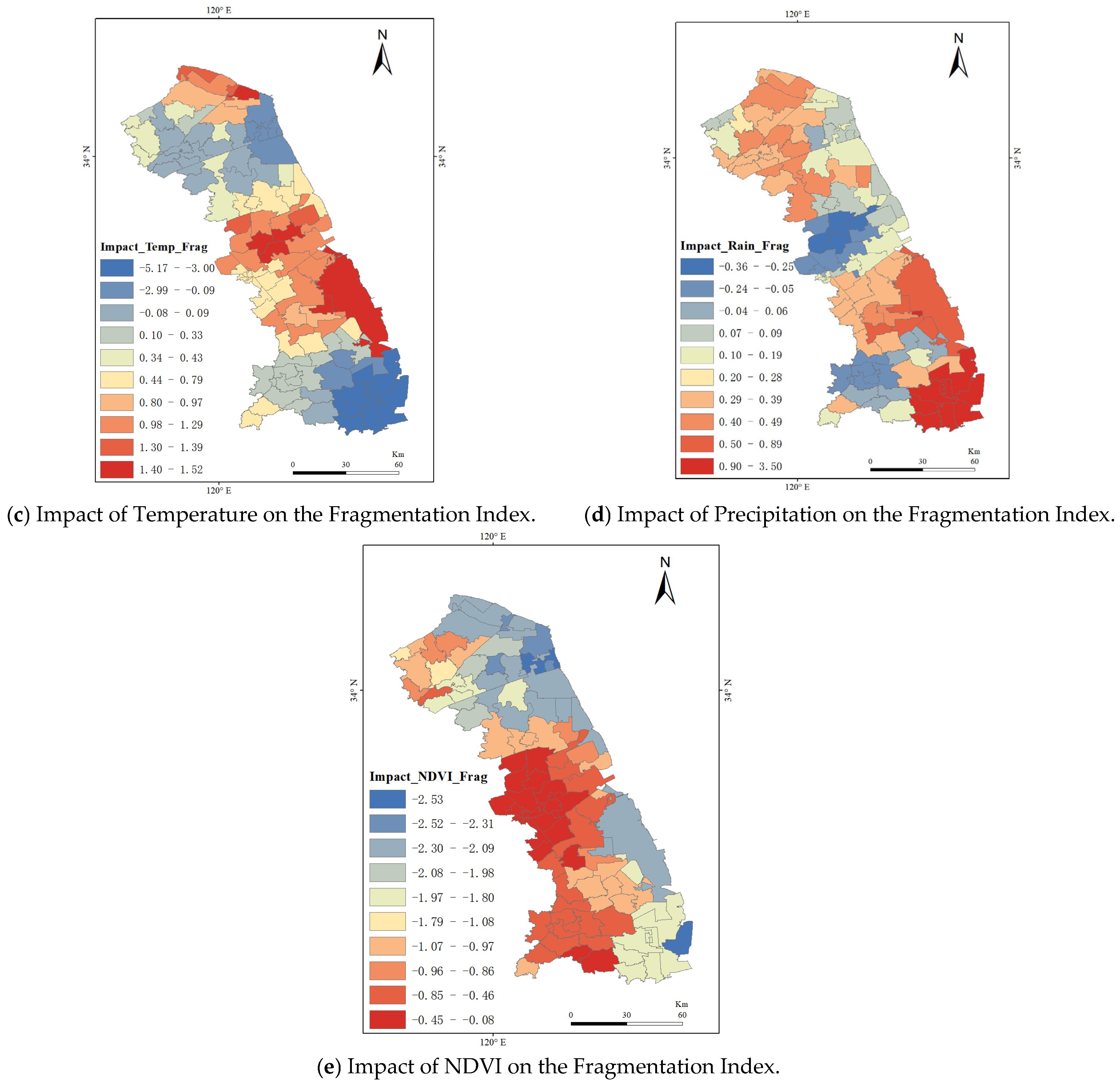
By visualizing the local regression coefficients of each explanatory variable (see Figure 4), the following spatial patterns and ecological implications are obtained:

(1) GDP: It exerts the strongest impact on LFI, showing a pattern of stronger influence along the coast and in the northern-southern regions and relatively weaker influence in the hinterland. The local coefficients are positive in some areas, reflecting that the increase in construction and industrial activities promotes landscape fragmentation; there are also negative coefficient areas, suggesting that when industrial efficiency and planning rationality are enhanced, economic growth does not necessarily lead to increased fragmentation. The shift from positive to negative coefficients across space indicates that the relationship between economic development and fragmentation is context-dependent.

(2) Population density: The overall performance is non-linear growth, with significant north–south differences and urban agglomeration effects. In urban areas with dense populations and complete facilities, landscape fragmentation is relatively low; in urban expansion belts and transportation corridors, positive local impacts emerge, indicating the need for refined land management to avoid “low-density sprawl”. The coefficient signs vary from negative to positive across the study area, suggesting that the fragmentation effect of population density is not uniform.

(3) NDVI: Most coefficients are negative, and the inhibitory effect is stronger in coastal wetlands and southern regions with good vegetation continuity. This indicates that improving vegetation coverage and connectivity can effectively mitigate fragmentation.

(4) Climatic factors (temperature, precipitation): Their overall effects are weak with insignificant spatial differences. They are more likely to indirectly affect fragmentation by influencing vegetation growth and hydrological processes; however, attention should still be paid to their interaction effects with extreme climates in specific years or local areas.

4. Discussion

(1) Spatial Differences and the Dominant Role of Human Activities

The Landscape Fragmentation Index (LFI) reveals significant disparities in fragmentation levels among counties in the study area, with the northern region and coastal fringes being more susceptible to external disturbances and thus exhibiting high fragmentation levels. This finding aligns with the expansion of construction land outside protected areas and the extension of transportation corridors [32]. Comparable patterns have been observed in other coastal wetland systems internationally. For example, studies on the Mediterranean coastal wetlands of Spain’s Ebro Delta have documented similar fragmentation trends driven by agricultural increase and tourism infrastructure development [11], while research on the Florida Everglades has highlighted how water management infrastructure, rather than population density per se, serves as the primary fragmentation driver [10]. These international comparisons suggest that while the specific drivers may vary, the general pattern of human activities as dominant agents of fragmentation holds across different geographic and socio-economic contexts [12]. Further results from the Generalized Additive Model (GAM) indicate that social system variables have the strongest explanatory power, confirming that human activities are the direct driver of wetland landscape fragmentation: rising population density is often accompanied by the outward expansion of residential, transportation, and service facilities, which encroach on wetland fringes and undermine landscape connectivity [33]. In the agricultural sector, increases in sown area and total output imply higher cultivation intensity and greater spatial occupation, leading to the fragmentation and replacement of original wetland patches. Pond aquaculture features a high-density grid layout, creating a significant spatial barrier effect. When combined with intensive agricultural practices, this effect exerts an amplified impact on landscape connectivity.

(2) Regulatory Effects and Threshold Characteristics of Ecological Context

Among ecological factors, the nonlinear relationship between the Normalized Difference Vegetation Index (NDVI) and LFI is prominent: high vegetation coverage and continuity can mitigate fragmentation and stabilize habitat structures, whereas vegetation degradation or intensified anthropogenic disturbances trigger a rapid escalation of fragmentation [34]. Precipitation influences wetland area as well as the position and stability of water-land boundaries by altering hydrological conditions: drought years tend to induce wetland contraction and bare land exposure, while extreme rainfall events may cause local flooding and herbaceous vegetation degradation, reflecting a bidirectional disturbance mechanism. Overall, the role of ecological factors is more inclined to be “regulatory-threshold”, with the intensity of their effects varying across temporal and spatial contexts.

(3) Directional and Structural Effects of Economic Magnitude Variables

The combined results of GAM and Geographically Weighted Regression (GWR) show that regional gross domestic product, general public budget revenue, and industrial gross output value index are mostly negatively correlated with LFI. This does not negate the pressure of economic growth on ecosystems but rather suggests that when fiscal investment is tilted toward ecological governance and industrial structures are adjusted toward greening and increase, economic magnitude can indirectly curb fragmentation through institutional and technological pathways [35]. Conversely, in the absence of aggregate constraints, consumption expansion and high-intensity fishery production may still elevate the risk of landscape fragmentation. Therefore, the impact of economic development on fragmentation is structurally dependent [36].

(4) Assumptions Underlying the LFI and Implications for Its Spatial Interpretation

A fundamental methodological consideration in this study is that the LFI—constructed using Cov-AHP with weights derived from the global covariance structure of PD, ED, DIVISION, and SHDI—assumes that the covariance structure is spatially invariant across the entire study area. If the relationships among PD, ED, DIVISION, and SHDI vary spatially, then the composite index may carry different ecological meanings in different sub-regions, which would complicate the interpretation of subsequent GWR coefficients. To address this concern, we conducted a sensitivity analysis by partitioning the study area into three latitudinal sub-regions (northern: Xiangshui + Binhai; central: Sheyang + Tinghu; southern: Dafeng + Dongtai) and recalculating the covariance structure for each sub-region. The Spearman rank correlation coefficients between the sub-regional covariance structures and the global covariance structure ranged from 0.82 to 0.91 (all p < 0.01), indicating that the covariance structure is relatively stable across the study area. This suggests that the LFI has a broadly consistent ecological meaning across different spatial units, supporting the validity of the subsequent GWR analysis.

(5) Management Implications for the Ramsar and World Heritage Site

The findings of this study have direct implications for the management of the Yancheng coastal wetlands as a Ramsar site and a UNESCO World Heritage site. First, the identification of social factors (particularly population density and agricultural intensity) as dominant drivers suggests that management strategies should prioritize land-use planning and agricultural policy over purely ecological interventions. Second, the spatially heterogeneous effects revealed by GWR indicate that a one-size-fits-all management approach is unlikely to be effective; instead, zonal management strategies tailored to the specific conditions of each sub-region are needed. For the northern sub-region (Xiangshui, Binhai), where fragmentation is high and coastal development intensity is increasing, priority should be given to controlling construction land expansion and establishing ecological buffer zones. For the southern sub-region (Dafeng, Dongtai), where fragmentation is moderate but agricultural and fishery activities are intensive, coordinated total quantity control and connectivity restoration should be promoted. Third, the threshold effects of NDVI and precipitation suggest that early warning systems based on these indicators could be developed to trigger timely intervention when fragmentation risks escalate.

(6) Uncertainties and Research Prospects

This study has identified and addressed major spatial issues using GAM and GWR, but there remains room for improvement. The use of administrative units as the basic analytical unit does not perfectly align with ecological boundaries (e.g., wetland habitat patches or bird migration corridors). Future research could adopt ecological units (e.g., watersheds, habitat patches) as the analytical basis when finer-scale ecological data become available. Future research could incorporate spatial error models, spatial lag models, or multiscale geographically weighted regression to characterize the non-stationary effects and scale differences across different geographic units. Additionally, considering the time-lag effects and mediating/moderating pathways of Economic–Social–Ecological variables and integrating panel data with instrumental variable methods would enhance causal interpretation. These improvements will provide more operable evidence for habitat restoration, ecological corridor planning, and zoned management and control.

5. Conclusions

The comprehensive Landscape Fragmentation Index (LFI) constructed using the Cov-AHP method indicates that the overall fragmentation of the study area showed a slow upward trend from 2010 to 2022, with a spatial pattern characterized by higher fragmentation in the north than in the south and higher levels in coastal areas than in inland regions. Areas with high fragmentation significantly overlapped with the expansion of construction land, and the inter-county differences remained stable. Among them, Xiangshui and Dafeng have long been at a high fragmentation level, while Tinghu has witnessed a notable increase, suggesting that the connectivity of local areas has been continuously weakened and ecological vulnerability has been heightened.

The Generalized Additive Model (GAM) reveals significant nonlinear relationships between landscape fragmentation and various influencing factors. Population density, crop sown area, total crop output, annual precipitation, and the Normalized Difference Vegetation Index (NDVI) are identified as the key variables. The interaction term of aquatic product output × total crop output is significant, indicating that the superposition of agricultural and fishery intensity will amplify the risk of fragmentation. Some economic and social variables exhibit stable linear effects on landscape fragmentation.

A comprehensive analysis of GAM and Geographically Weighted Regression (GWR) results shows that social system factors (population and agricultural intensity) are the dominant drivers of fragmentation, while ecological factors (NDVI and precipitation) play regulatory and threshold roles. Social factors have the strongest explanatory power, followed by ecological factors. The impact of economic factors on fragmentation is directional and structurally dependent. Gross Domestic Product (GDP) and NDVI are the factors with the strongest spatial heterogeneity; their regression coefficients vary across the study area, with positive and negative values observed in different sub-regions, reflecting the spatially non-stationary nature of their effects. They have the potential to demonstrate negative regulation against the backdrop of green transformation and fiscal investment in ecological governance.

In areas where high fragmentation overlaps with high coefficient values, it is necessary to impose constraints on construction intensity and prioritize the layout of ecological buffer zones. In regions experiencing rising population-agricultural intensity or implementing integrated fishery-agriculture practices, coordinated total quantity control and connectivity restoration (corridor/patch restoration) should be promoted. Efforts should be intensified to maintain the connectivity and integrity of coastal wetland patches, with a focus on controlling the expansion of construction land in coastal high-fragmentation zones. Threshold values of NDVI and precipitation should be used to guide the implementation of temporal disturbance control measures so as to improve landscape connectivity and habitat quality. In this way, the quality of wintering habitats for rare waterbirds such as red-crowned cranes can be indirectly enhanced, serving the long-term protection and restoration of red-crowned crane wintering grounds.

The integrated “Cov-AHP + GAM + GWR” framework developed in this study is potentially transferable to other coastal wetland regions facing similar fragmentation pressures, particularly those requiring the integration of multi-source data, identification of nonlinear driving relationships, and revelation of spatial heterogeneity. However, several caveats should be noted when applying this framework to other contexts. Cov-AHP weights depend on the covariance structure among the selected landscape metrics; different wetland types (e.g., freshwater marshes, mangroves, peatlands) may require adjustments to the indicator system. GAM and GWR also have certain sample size requirements; results should be interpreted with caution when applied to small-sample or data-scarce regions. Overall, the strength of this framework lies in its systematicity and flexibility, offering a reference methodological paradigm for landscape fragmentation research in coastal wetlands globally.