A Comparative Assessment of Machine and Deep Learning Approaches for Grassland Mapping with Sentinel-1, Sentinel-2 and Ancillary Data

Abstract

Grasslands represent one of the most extensive terrestrial biomes globally, covering approximately one-third of the Earth’s land surface, yet they are increasingly threatened by land-use change and overgrazing, underscoring the need for reliable monitoring approaches. This study compares the performance of machine learning and deep learning algorithms for grassland mapping using multi-source remote sensing data derived from Sentinel-1, Sentinel-2, and terrain variables. The research was conducted in Mpumalanga Province, South Africa, a heterogeneous landscape comprising lowland savannas, high-altitude grasslands, escarpments, and riverine wetlands. Random Forest (RF) and Support Vector Machine (SVM) classifiers were implemented in Google Earth Engine using fused satellite and terrain datasets with field-collected samples for training and validation, while a One-Dimensional Convolutional Neural Network (1D-CNN) was developed in Python 3.13.5 using the same inputs. Results demonstrate that integrating multi-source data improves classification accuracy, with radar-based features contributing the most. RF achieved the highest performance, with an overall accuracy of 97.7% and grass-class precision, recall, and F1-score exceeding 0.97, closely followed by the 1D-CNN with 91% overall accuracy and complete grass detection. In contrast, SVM performed notably lower with an overall accuracy of 80,8%. These findings highlight the effectiveness of advanced learning approaches for grassland mapping and support their application in ecological restoration and environmental management.

1. Introduction

Grasslands represent one of the most vital ecosystems globally, as they cover nearly one-third of the land surface [1,2,3]. They represent approximately 40% of the distributed land cover on Earth. Grasslands serve as a major source of food for livestock grazing, which is essential for the production of goods such as protein, fertilizer, leather and fiber [4,5]. Additionally, grasslands are important for biodiversity reserves, recreational and cultural needs, water catchments, and carbon sequestration [6,7,8]. In South Africa, grassland covers approximately one-third of the country, with the broad units comprising the dry and mesic high-veld grasslands, sub-escarpment and Drakensberg grassland [9,10]. Grasslands cover approximately 349,174 km² in central South Africa, linking and extending into other key biomes such as thickets, Nama-Karoo, savannas, and forests [11]. In recent years, humans have greatly degraded various grasslands with events such as over-grazing, pollution and conversion to farmlands [12]. Additionally, severe weather phenomena such as sandstorms, rainstorms, fires and frost have affected grasslands, leading to a decline in soil fertility and moisture retention capability and ultimately resulting in desertification [12,13]. These mounting threats to grasslands highlight the urgent need for advanced monitoring tools such as remote sensing to track degradation and guide restoration.

Remote sensing emerges as a powerful solution to monitor vast, dynamic grassland ecosystems efficiently and at scale. Remote sensing offers significant advantages for monitoring grassland ecosystems, including high-resolution spatial data, frequent temporal coverage to capture landscape heterogeneity and dynamic changes, and the ability to quantify transformations, grazing impacts, grassland types, disturbances such as drought and wildfires, and support conservation efforts [14,15]. Optical sensors such as Moderate Resolution Imaging Spectroradiometer (MODIS), Landsat, Satellite Pour l’Observation de la Terre (SPOT), and Sentinel-2 deliver extensive spectral bands for productivity [16,17]. Additionally, SAR data from Sentinel-1 and Advanced Land Observing Satellite (ALOS) enable cloud-independent acquisition for consistent seasonal monitoring, assess structural and biophysical attributes, and supply auxiliary topographic and soil indices to enhance model precision when fused with optical data [16]. However, challenges persist from the grassland biome’s vast spatial extent and ecological complexity, which historically complicated accurate mapping, alongside potential limitations in optical data due to cloud cover and the need for sensor integration to fully address grassland dynamics [5]. Overcoming these challenges calls for cloud-based platforms like GEE to process massive remote sensing datasets and enable precise grassland assessments.

The use of platforms such as GEE has progressed over the past few years, making it easy to process large-scale datasets [18,19]. GEE is a cloud-centric platform designed for large-scale geospatial analysis [18,20,21]. This platform stores satellite images and can manage large datasets [22,23,24]. It simplifies the processing of data, allowing scientists and specialists to monitor and assess grasslands on a larger scale and frequency. GEE has the capacity to analyze and process large-scale remote sensing data and utilize custom algorithms that allow for the effective monitoring of agricultural land, urban expansion and wildfires that pose a threat to grasslands. Hence, this study intends to employ GEE for grassland assessments in the low-veld region of South Africa. Several studies investigated the effectiveness of GEE in monitoring and mapping woody vegetation [18,20,25,26]. Ref. [27] used a GEE web-based application and MODIS-derived Enhanced Vegetation Index (EVI) products to map vegetation on a global level in Vietnam; this study successfully documented changes in vegetation quality and the impact of Vietnam’s government mitigation measures. In a related study by [25], a machine learning framework was utilized with Sentinel-2 data to identify sea grasses in the Iron and Aegean area. The inter-annual and seasonal fluctuations of sea grass up to 40 m depth were successfully mapped using this approach. Ref. [28] did a study on tropical savanna grasslands mapping and monitoring in Sabu Island, Indonesia, using Sentinel-2A Level-1C imagery. Their findings suggest that the Sentinel-2-derived Normalized Difference Vegetation Index (NDVI) from GEE can efficiently and accurately detect grasslands and observe tropical savanna grasslands. In the study, Sentinel-2A images were used to classify grassland, achieving an overall accuracy of 82.86%. Similar approaches using Sentinel-1- and Sentinel-2-derived indices from GEE could be applied in South Africa to efficiently and accurately detect changes in grasslands. GEE’s support for custom algorithms facilitates seamless integration with machine learning methods, thereby enhancing classification accuracy for heterogeneous grassland ecosystems.

Machine learning techniques have become increasingly important in land cover classification due to their ability to handle high-dimensional and complex datasets efficiently. Widely used algorithms include RF, SVM, and XG Boost [29,30,31]. For example, Ref. [31] showed that the integration of RF with PROBA-V imagery substantially improves grassland classification in Central Africa by more effectively representing spectral variability within heterogeneous landscapes. Similarly, Ref. [30] reported that the SVM outperformed alternative classifiers when applied to Sentinel-2 time series data, primarily due to its capability to model complex non-linear relationships and exploit phenological information for accurate mapping of grassland plant communities. Among these, the RF algorithm is particularly favored because it requires minimal parameter tuning, is computationally efficient, and has demonstrated strong performance in tasks such as grassland and crop classification. Although machine learning methods generally achieve high classification accuracy, their effectiveness often depends on the use of a large number of input features [32,33]. Therefore, the careful selection and optimal combination of relevant features play a crucial role in improving overall model performance.

Following the advancements in machine learning, deep learning approaches have emerged as powerful tools for land cover classification, particularly in complex environments. Deep learning models, such as Convolutional Neural Networks (CNN) and Recurrent Neural Networks (RNN), are capable of automatically learning hierarchical feature representations directly from raw data, reducing the need for manual feature engineering. These models have demonstrated superior performance in capturing spatial and temporal patterns within high-resolution and multi-temporal remote sensing datasets, making them particularly suitable for detailed grassland mapping and vegetation analysis [34,35,36]. Deep CNNs have demonstrated competitive performance in land cover classification due to their ability to detect local spatial correlations and their ability to handle multi-scale resolution images [37]. However, despite their advantages, deep learning methods typically require large volumes of labeled training data and substantial computational resources for model training and optimization [38]. Additionally, their complexity can limit interpretability compared to traditional machine learning algorithms. Nevertheless, with the increasing availability of high-quality satellite imagery and advances in computational capacity, deep learning continues to show significant potential for improving classification accuracy and advancing remote sensing applications [39]. Despite these advancements, existing gaps in grassland monitoring underscore opportunities for innovative approaches.

Important gaps remain in remote sensing-based monitoring of grassland ecosystems, particularly in the limited integration of multi-source data fusion and the underutilization of deep learning methodologies for grassland-specific applications. Most existing studies rely on either optical data (e.g., Sentinel-2) or SAR data (e.g., Sentinel-1) independently, thereby neglecting the synergistic potential of their integration for improving grassland classification performance [40,41]. Although multi-source data fusion has demonstrated strong performance in agricultural applications such as improved nitrogen estimation in winter wheat [42] and high-accuracy crop classification using Sentinel-1, Sentinel-2, and Landsat-8 data [43,44,45], its application in grassland environments remains limited and less systematically evaluated.

In addition, traditional machine learning algorithms such as RF and SVM are widely used in grassland modeling and classification [44,46,47,48], while deep learning approaches (e.g., CNNs, transformers, and hybrid architectures) remain underexplored due to data limitations and the structural complexity of grassland ecosystems [49]. This limitation is particularly relevant in grassland and non-grassland discrimination, where high spectral similarity, seasonal variability, and spatial heterogeneity increase classification uncertainty and reduce model separability. Although deep learning has been successfully applied in agricultural vegetation and species-level classification [50,51,52], its effectiveness in grassland-specific mapping remains insufficiently investigated [53]. Accordingly, there is still a lack of studies that systematically evaluate and compare machine learning and deep learning approaches under a unified multi-source framework for grassland classification in complex environments.

This study aims to perform a comprehensive classification of grassland ecosystems by integrating data from Sentinel-1 and Sentinel-2. Through the combination of these complementary datasets, the study seeks to improve the accuracy and robustness of grassland mapping. To achieve this, deep learning algorithms will be employed to analyze and classify the satellite imagery. The workflow will be primarily implemented within the GEE platform, leveraging its cloud-based access to satellite imagery and robust geospatial processing capabilities. While multiple machine learning algorithms were evaluated, emphasis was placed on identifying and comparing the strongest conventional machine learning classifier against the deep learning approach. RF and SVM models will be trained directly within GEE for classification tasks. In parallel, a deep learning model will be developed and trained externally using Python. Ultimately, the study aims to contribute to more precise monitoring and management of grassland resources, which are critical for biodiversity conservation, agriculture, and climate resilience.

The specific objectives are:

• To integrate multi-source geospatial data, including Sentinel-1 SAR, Sentinel-2 multispectral imagery, and terrain variables for enhanced feature representation in grassland classification.
• To develop and compare the performance of a traditional machine learning model, RF, with a 1D-CNN deep learning model for classifying grassland cover.
• To identify the most accurate and generalizable model for grassland mapping by evaluating classification outputs using statistical metrics and validation against ground truth data.

2. Materials and Methods

2.1. Description of the Study Area

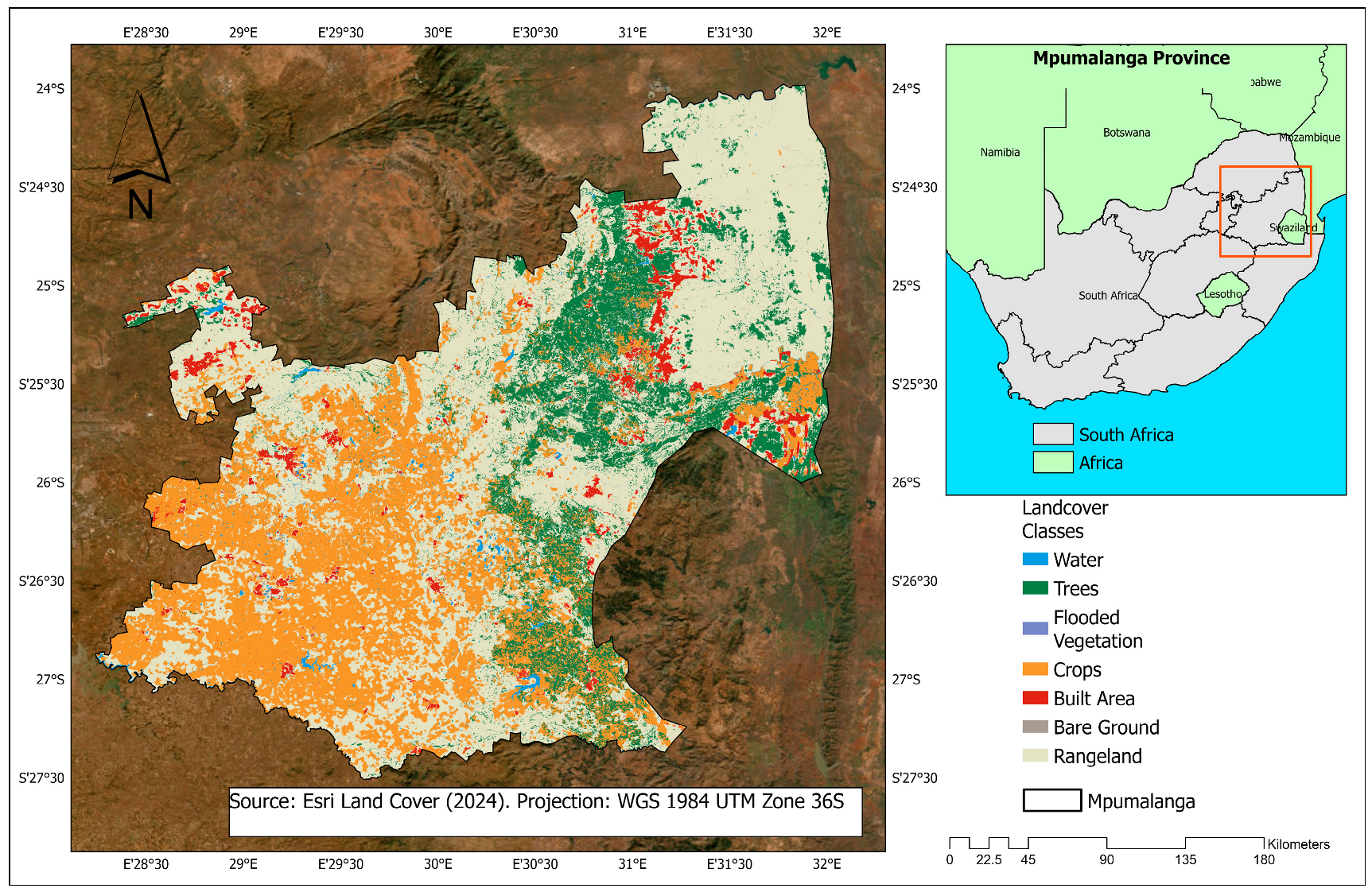
The study area is Mpumalanga Province, located in the north-eastern part of South Africa (Figure 1). Grassland biome coverage in Mpumalanga accounts for approximately 61% of the province, covering an estimated area of 47,810 km². Of this area, nearly 44% has undergone significant transformation due to the removal or substantial alteration of indigenous vegetation [54,55]. The grasslands in Mpumalanga are predominantly found in fertile soils, making them highly productive yet vulnerable. Major threats to grassland conservation include open-cast coal mining activities, agricultural expansion, invasive alien plant species and commercial plantation forestry. The biome can be broadly categorized into high-altitude mountain grasslands found in the Highveld, which support a rich diversity of endemic species, and the lower-altitude Lowveld grasslands, which are more widespread and adapted to warmer conditions with fewer endemics [54]. Mpumalanga is characterized by varying temperature and precipitation ranges, with distinct summer (December to February), autumn (March to May), winter (June to August) and spring (September to November) months. The region receives the majority of its annual rainfall, ranging between 800 and 1600 mm, during the summer season, which spans from November to March [56,57]. The Lowveld Escarpment region receives the highest levels of precipitation, with orographic rainfall accounting for most of the precipitation during the drier seasons [57].

2.2. Dataset

2.2.1. Satellite Data

Sentinel-1 and Sentinel-2 images were downloaded from GEE. The Sentinel-1 collection in GEE comprises Sentinel-1 Ground Range Detected (GRD) scenes, which have been calibrated and ortho-corrected by the Sentinel-1 Toolbox [58,59]. The Sentinel-1 mission provides Synthetic Aperture Radar (SAR) data in the C-band (C-SAR), offering mode-dependent spatial resolutions of approximately 5 m and a revisit interval of around three days over the study area. A key advantage of SAR technology is its ability to acquire data under all-weather conditions, including cloud cover and nighttime, ensuring consistent temporal coverage. For this study, S-1 C-SAR data were obtained as Level-1 Ground Range Detected (GRD) products with dual polarization (VV and VH) through the GEE platform. Sentinel-1 Polarization bands to be used include VH and VV backscatter coefficients. Several studies have indicated that the VV backscatter coefficient facilitates detailed analysis of characteristics such as vegetation and soil moisture [60]. In contrast, the VH backscatter coefficient is recognized for its high sensitivity to vegetation, while demonstrating relatively lower sensitivity to factors like topography compared to the VV polarization [61].

The Sentinel-2 (S-2) has 13 optical spectral bands: coastal aerosol (Band 1), blue (Band 2), green (Band 3), red (Band 4), red-edge 1 (Band 5), red-edge 2 (Band 6), red-edge 3 (Band 7), near-infrared (Band 8), narrow near-infrared (Band 8A), water vapor (Band 9), shortwave infrared 1 (Band 11), shortwave infrared 2 (Band 12), and the cirrus band (Band 10). Three of these bands-Bands 5, 6, and 7 are located in the red-edge region, which is particularly valuable for vegetation analysis [62,63,64]. The spatial resolution varies by band, ranging from 10 m, 20 m and 60 m. The satellite offers a revisit frequency of approximately three days over the study area, enabling frequent and detailed monitoring. For this study, only the 10 m and selected 20 m bands were utilized. Specifically, Bands 1 (Coastal aerosol), 9 (Water vapor), and 10 (Cirrus/SWIR) were excluded due to their limited relevance to vegetation classification.

The Shuttle Radar Topography Mission (SRTM) digital elevation model was used to derive the slope, elevation and aspect.

2.2.2. Field Data

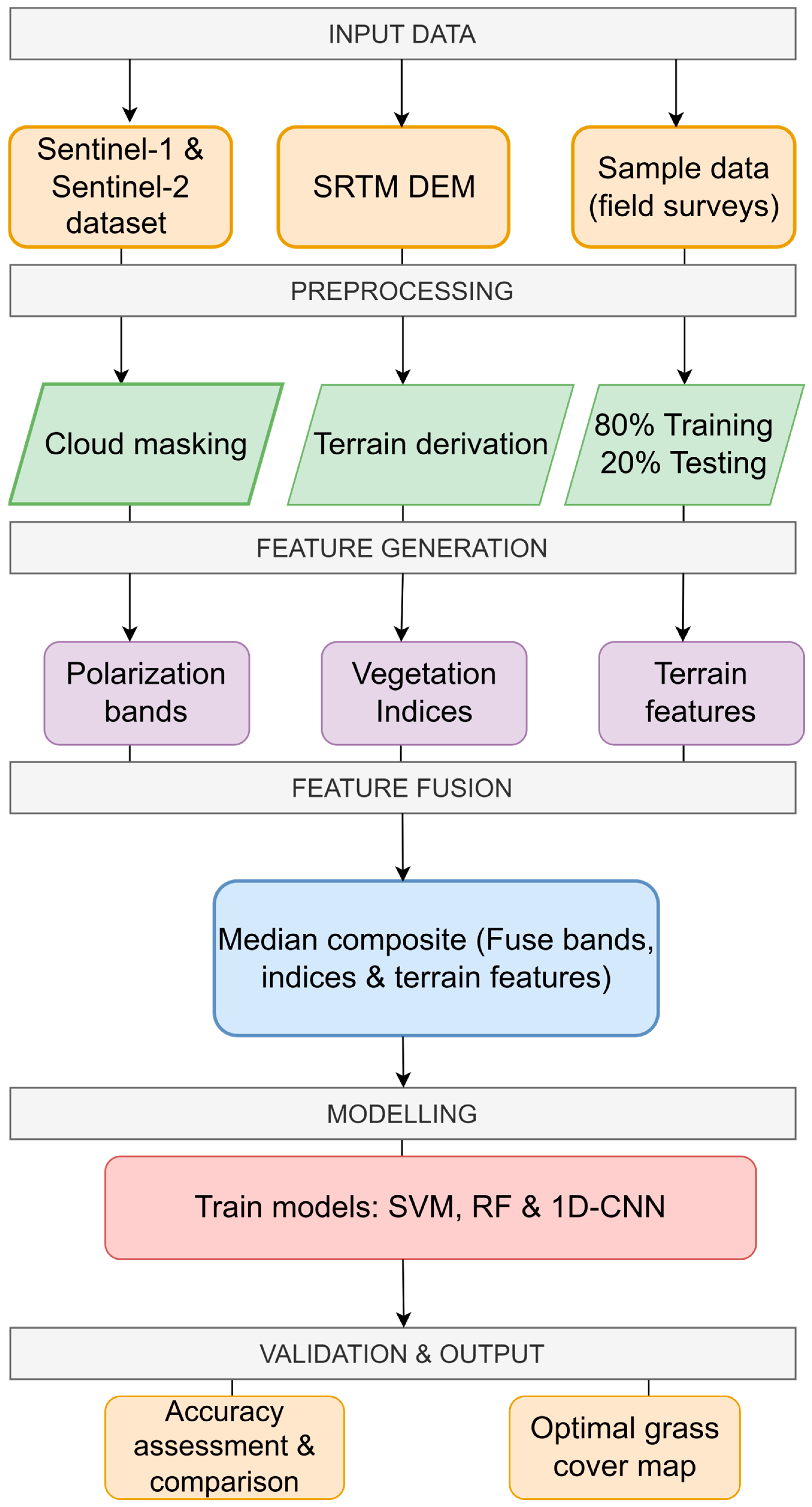
Field sample points were collected randomly in the grassland biomes of Mpumalanga Province, stratified by major ecoregions and elevation gradients to ensure spatial and ecological representativeness. ArcGIS Survey 123 version 3.19.114 was used to collect coordinates, with a minimum distance of 100 m enforced between points to reduce spatial autocorrelation. Data collection was conducted between June and December 2024, using randomly selected sampling points, each situated within 1 km × 1 km field survey plots. Each plot served as a spatial unit for data collection, ensuring coverage across representative grassland areas within the province. The timing of field sampling was aligned with the acquisition dates of Sentinel satellite imagery to ensure optimal data calibration and integration. The reference data collected during field surveys was used as training (80%) and testing data (20%) [63]. The field datasets were classified into grassland and non-grassland land cover classes, containing 816 grass samples and 573 non-grass samples, indicating a moderate class imbalance. To minimize potential bias associated with unequal class representation, stratified train-test splitting was applied to preserve class proportions during model training and validation. Additionally, precision, recall, kappa coefficient, F1-score metrics and 10-fold cross-validation were incorporated alongside overall accuracy to provide a more balanced assessment of model performance across classes, as shown in Figure 2.

2.3. Classification System

This study employs a binary classification approach, distinguishing between grass and non-grass classes. The adopted scheme aids in improving classification accuracy by reducing misclassification that might occur in a multiclass system that has spectrally similar vegetation types. Additionally, other ecological and remote sensing studies use this approach as a baseline for assessing grassland extent, fragmentation and degradation trends [65,66,67].

2.3.1. Vegetation Indices and Terrain Features

The vegetation indices employed in this study include the Normalized Difference Vegetation Index (NDVI), which captures physiological, structural and biochemical attributes of the vegetation canopy; the Soil-Adjusted Vegetation Index (SAVI), which accounts for soil background effects; and the Enhanced Vegetation Index (EVI), which improves sensitivity to canopy structure and minimizes atmospheric influences. Additionally, the Normalized Difference Red Edge Index (NDRE) estimates chlorophyll content in mature vegetation, while the Green Chlorophyll Index (GCI) complements NDRE by detecting chlorophyll dynamics in less dense vegetation (

Table 1. Vegetation indices used in this study.

Vegetation Index	Equation	Citation
Normalized Difference Vegetation Index (NDVI)	(NIR − Red)/(NIR + Red)	[71]
Soil-Adjusted Vegetation Index (SAVI)	((NIR − Red)/(NIR + Red + L)) ∗ (1 + L)	[72]
Enhanced Vegetation Index (EVI)	G ∗ ((NIR − Red)/(NIR + C1Red − C2Blue + L))	[73]
Normalized Difference Red-Edge index (NDRE)	(NIR − RedEdge)/(NIR + RedEdge)	[74]
Green Chlorophyll Index (GCI)	GCI = (NIR/Green) − 1	[75]

). Together, these indices represent complementary dimensions of vegetation condition: structure, greenness, and physiological status, thereby improving class separability and enhancing model accuracy in grassland classification [63,68,69,70].

Elevation, slope and aspect were extracted using the SRTM DEM on GEE. Terrain features serve as valuable auxiliary predictors for distinguishing spectrally similar land cover classes, such as grass and shrub, which often occupy distinct topographic zones. They also help resolve spectral ambiguities between grass, sparse shrub cover and bare soil. Terrain features aid machine and deep learning classifiers in separating these.

2.3.2. Feature Construction

The feature dataset used to map grassland distribution in the study area comprised 21 selected variables, including spectral bands, vegetation indices, terrain components and radar-derived features as shown in

Table 2. Overview of features selected for the study.

Category	Feature	Feature Number
Spectral bands	Blue, green, red, red edge 1, red edge 2, red edge 3, NIR, Narrow NIR, red edge 4, SWIR 1, SWIR 2	11
Vegetation Indices	NDVI, SAVI, EVI, NDRE, GCI	5
Terrain	Slope, aspect, elevation	3
Radar	VV, VH	2

. All features were derived and computed using the Google Earth Engine (GEE) platform.

2.3.3. RF Classification

The RF algorithm has demonstrated high effectiveness and broad applicability in land use classification, ecosystem mapping and habitat delineation [5,66,76,77]. The algorithm reduces noise and outliers, provides a high classification accuracy, has a capacity to process large datasets simultaneously, and reduces overfitting [66]. To optimize the performance of the RF classifier in the current study, a grid search was conducted across key hyperparameters. The number of trees was varied across four levels: 10, 20, 50, and 100. The maximum number of terminal nodes was tested using values of: (no constraint), 10, 20, and 30. Minimum leaf population was adjusted to 1, 5, and 10 to control overfitting by regulating node purity. Additionally, the number of variables considered at each split was tuned using values of: (default behavior), 3, and 5. This tuning strategy aimed to identify the optimal parameter combination that maximized classification accuracy while maintaining model generalization [69]. Feature importance scores were visualized and plotted to assess the relative contribution of each variable to the classification outcome.

2.3.4. SVM Classification

SVM algorithm has been extensively employed in remote sensing classification owing to its robust generalization capacity, effectiveness in handling high-dimensional datasets, and capability to address non-linear classification problems through kernel-based learning [44,47]. In the present study, hyperparameter optimization was undertaken to enhance SVM performance and strengthen model generalization. A grid search procedure was implemented to systematically evaluate combinations of kernel functions and parameter settings. Two kernel types, namely, Linear and Radial Basis Function (RBF), were examined. For the cost parameter (c), values of 1, 10, and 100 were tested, while gamma values of 0.1, 0.5, and 1 were assessed for the RBF kernel. This tuning strategy was designed to identify the optimal parameter configuration that maximized classification accuracy while mitigating risks of overfitting. The optimized SVM model was subsequently evaluated using multiple performance metrics, including overall accuracy, precision, recall, F1-score, and the kappa coefficient, thereby ensuring a comprehensive assessment of classification reliability and robustness.

2.3.5. 1D-CNN Classification

Deep learning algorithms are characterized by enhanced generalization capabilities and stronger predictive power, enabling the model to address complex tasks across domains such as image recognition, speech processing, and machine translation [78]. Within this paradigm, CNNs have proven particularly effective for hyperspectral image classification, as they can efficiently extract spectral–spatial features. Although CNN architectures are commonly associated with image-based spatial analysis, 1D-CNNs have also demonstrated strong performance for structured tabular and spectral datasets, as they can effectively learn local feature interactions and nonlinear relationships among ordered input variables [79,80,81]. In this study, the predictor dataset consisted of ordered multi-source remote sensing features, including spectral bands, vegetation indices, SAR variables, and terrain attributes. The sequential arrangement of these variables made 1D-CNN a suitable architecture for evaluating deep learning performance on fused remote sensing predictors while maintaining relatively low computational complexity compared to more advanced deep learning architectures.

CNNs have become one of the most widely adopted approaches in this field, with numerous studies confirming their ability to achieve high classification accuracy [79,80,81]. For example, Ref. [82] used a 1D-CNN architecture for hyperspectral data classification, comprising an input layer, a convolutional layer, a max-pooling layer, and a fully connected layer. This design demonstrated strong feature extraction capabilities and improved classification performance. Similarly, Ref. [83] compared multiple models for estimating canopy nitrogen in grasslands and found that the 1D-CNN achieved superior accuracy relative to partial least squares regression (PLSR) and Gaussian process regression (GPR). Furthermore, Ref. [84] evaluated three classifiers, Conv1D, Attention Long Short-Term Memory (At-LSTM), and RF, to identify native grasslands and their phenological stages. Their findings revealed that the Conv1D-based model achieved the highest overall accuracy (OA = 0.88), showing the effectiveness of deep learning models in remote sensing. This study used 1D-CNN to evaluate its potential in grassland classification.

The CNN architecture consisted of two one-dimensional convolutional layers with 32 and 64 filters, respectively, each using a kernel size of 3 and Rectified Linear Unit (ReLU) activation. Max-pooling and adaptive average-pooling layers were incorporated to reduce dimensionality and improve feature extraction efficiency. A fully connected layer with dropout regularization (0.3) was included to minimize overfitting and improve model generalization. The model was trained for 25 epochs using a batch size of 256, the Adam optimizer with a learning rate of 0.001, and binary cross-entropy loss with logits (BCEWithLogitsLoss). Classification performance was evaluated using overall accuracy, confusion matrix, precision, recall, F1-score, and Cohen’s kappa coefficient to ensure consistency with the machine learning model assessments (

Table 3. Summary of 1D-CNN architecture.

Category	Configuration
Conv1D Layer 1	32 filters, kernel size = 3, ReLU activation
Max Pooling	MaxPool1d (kernel size 2)
Conv1D Layer 2	64 filters, kernel size = 3, ReLU activation
Global Pooling	Adaptive average pooling (output size = 1)
Fully Connected Layers	64➛32➛1, ReLU + Dropout (0.3)
Optimizer	Adam, learning rate = 0.001
Loss Function	Binary Cross-Entropy (BCEWithLogitsLoss)
Training Parameters	25 epochs, batch size = 256
Evaluation Metrics	Accuracy, Confusion Matrix, Precision, Recall, F1-score, Kappa coefficient, 10-fold cross-validation

). The implemented 1D-CNN comprised 8449 trainable parameters, distributed across two convolutional layers (128 and 6208 parameters, respectively) and two fully connected layers (2080 and 33 parameters).

2.3.6. Feature Combination

Five feature scenarios were designed to compare the performances of RF for different features, as shown in

Table 4. Feature scenarios designed in this study.

Category	Feature	Bands	Indices	Terrain	Feature Number
Exp 1	√				2
Exp 2		√			11
Exp 3			√		5
Exp 4				√	3
Exp 5	√	√	√	√	21

. To systematically assess the contribution of different feature types to classification performance, five distinct feature scenarios were designed and evaluated (Table 4). Experiment 1 utilized radar backscatter features (VV and VH) from Sentinel-1. Experiment 2 incorporated only spectral bands from Sentinel-2. Experiment 3 focused exclusively on vegetation indices. Experiment 4 included terrain variables comprising elevation, slope, and aspect derived from a digital elevation model. Finally, experiment 5 combined all available features—radar, spectral bands, indices, and terrain— into a comprehensive dataset to evaluate the synergistic effect of multi-source data fusion on classification accuracy. This full-feature scenario served as a benchmark to determine whether integrated feature sets yield superior performance compared to individual sources [85].

2.3.7. Accuracy Assessment

Accuracy assessment is a critical component in evaluating the reliability and robustness of classification results [86]. To evaluate the performance of the grassland classification models, four standard evaluation metrics were computed using the verification dataset: precision, recall, overall accuracy, F1 score, kappa coefficient, 10-fold cross-validation and McNemar’s test. Precision quantifies the proportion of correctly identified grass pixels among all pixels predicted as grass, while recall measures the ability of the model to correctly detect all actual grass pixels. The F1 score, as the harmonic mean of precision and recall, balances these two aspects. Overall accuracy reflects the proportion of correctly classified pixels across all classes, and it accounts for agreement occurring by chance, whereas the kappa coefficient measures classification agreement while accounting for agreement occurring by chance [66,85,87]. The closer the values of these indicators are to 1, the better the results of the grassland classification. Cross-validation constitutes a widely employed statistical technique for assessing model performance [41]. In this approach, the dataset is partitioned into k subsets, whereby the algorithm iteratively trains on one subset while validating on the remaining subsets. This repeated process yields accuracy scores for each fold, and the overall cross-validation estimate is obtained by averaging these values. To determine the relative effectiveness and statistical significance of the highest-performing machine learning model and 1D-CNN, McNemar’s test was applied [79]. McNemar’s test is a statistical test used to compare two paired binary outcomes, such as whether two classifiers make different correct/incorrect predictions on the same test cases [68].

3. Results

3.1. Accuracy Comparison Under Different Experiments (RF)

Classification performance across experiments varied in model accuracy and reliability, driven by differences in input features (

Table 5. Accuracies of different experiments.

	Precision	Recall	Overall Accuracy	F-1 Score
Exp 1	0.8931	0.8567	0.8759	0.8746
Exp 2	0.9453	0.9254	0.9361	0.9353
Exp 3	0.907	0.8853	0.8985	0.8961
Exp 4	0.8737	0.8308	0.8534	0.8517
Exp 5	0.9811	0.9774	0.9774	0.9792

). Exp 5 achieved the highest performance, with precision (0.9811), recall (0.9774), F1-score (0.9792), and overall accuracy (0.9774). This experiment combined Sentinel-1 radar backscatter (VV and VH), Sentinel-2 spectral bands and vegetation indices, and terrain-derived variables (elevation, slope, and aspect), enabling strong class discrimination in structurally and spectrally complex grassland environments. Exp 2 also performed strongly, with overall accuracy of 0.9361 and balanced precision (0.9453) and recall (0.9254). Exp 3 followed with 0.8985 accuracy, while Exp 1 and Exp 4 showed comparatively lower performance. Exp 1, which relied solely on Sentinel-1 VV and VH backscatter, achieved moderate accuracy (0.8759), indicating that radar alone can support classification but may lack spectral information. Exp 4, using only terrain features, yielded the lowest accuracy (0.8534), reflecting limited separability when relying solely on topographic data. These findings highlight the importance of multi-source data fusion in ecological classification, with structural, spectral, and terrain features contributing complementary information that enhances model performance.

3.2. Feature Importance

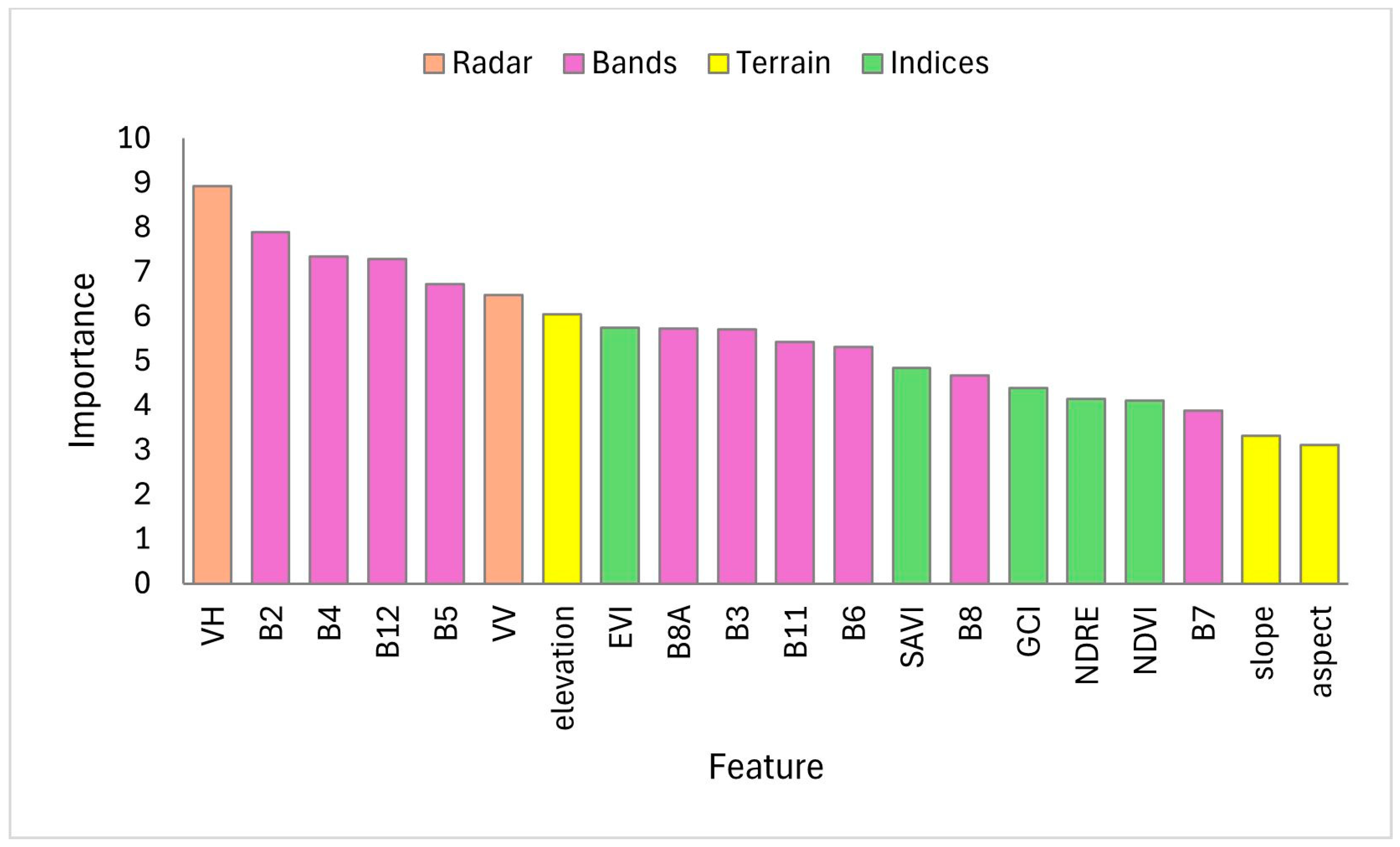
The feature importance ranking function was embedded within the GEE classification workflow to compute and visualize the relative contribution of each input variable. The resulting plot is presented in Figure 3, which displays the importance scores for all features utilized in the study, including Sentinel-1 backscatter, terrain-derived variables, Sentinel-2 spectral bands and indices. Feature importance analysis from Experiment 5 revealed that radar and spectral variables were the most influential in distinguishing grass from non-grass classes. The top-ranked feature was Sentinel-1 VH backscatter (importance = 8.93), which captures vegetation structure and volume. Sentinel-2 bands B2 (blue, 7.893), B4 (red, 7.344), and B12 (SWIR, 7.282) followed closely, indicating strong spectral separability in visible and shortwave regions. Red-edge band B5 (6.718) and VV backscatter (6.481) also contributed significantly, reinforcing the value of radar-optical fusion. Terrain elevation (6.041) ranked above several vegetation indices, suggesting that topographic gradients influence vegetation distribution and class separability. Among vegetation indices, EVI (5.745), SAVI (4.844), NDVI (4.119), and NDRE (4.142) showed moderate importance, reflecting their role in capturing canopy vigor and chlorophyll content. Additional spectral bands such as B8A (5.731), B3 (green, 5.71), B11 (SWIR, 5.435), and B6 (red-edge, 5.317) provided complementary information. Chlorophyll-related indices like GCI (4.386) and NDRE (4.142) added physiological information, though with lower relative impact. Terrain slope (3.318) and aspect (3.121) were the least influential, indicating that while topography contributes contextual information, it is less discriminative than radar and spectral features. These results confirm that integrating Sentinel-1, Sentinel-2, and terrain data enhances the classification model mapping accuracy.

3.3. Accuracy Assessment of Optimal Feature Dataset (RF)

The classification results demonstrated excellent performance in distinguishing between grass and non-grass areas. The confusion matrix yielded 155 true positives, 105 true negatives, 5 false positives, and 1 false negative, resulting in an overall accuracy of 97.74%. For the grass class, the model achieved a precision of 0.9688, recall of 0.9936, and F1-score of 0.9811, indicating that nearly all grass areas were correctly identified with minimal commission and omission errors. The non-grass class attained a precision of 0.9906, recall of 0.9545, and F1-score of 0.9722, reflecting strong classification performance with slightly higher omission errors relative to the grass class, as shown in

Table 6. Confusion matrix of the RF best classification.

Actual/Predicted	Grass	Non-Grass	Precision	Recall	F-1 Score
Grass	TP = 155	FN = 1	0.969	0.994	0.9811
Non-grass	FP = 5	TN = 105	0.991	0.955	0.9722
Overall accuracy					0.977
Kappa coefficient					0.953
Cross validation					96.90%

. Grid search identified the best RF configuration as 20 trees, with default settings for maximum nodes and variables per split, and a minimum leaf population of 1. These results suggest that the model effectively discriminates between the two land cover types with high consistency, low misclassification, and strong agreement across both producer and user perspectives.

3.4. Accuracy Results for 1D-CNN Optimal Feature Dataset

The CNN classification model demonstrated strong performance on the test dataset (n = 278). The confusion matrix indicated that 90 non-grass and 162 grass samples were correctly classified, while 25 non-grass samples and 1 grass sample were misclassified (

Table 7. Confusion matrix for 1D-CNN model.

Actual/Predicted	Grass	Non-Grass	Precision	Recall	F-1 Score
Grass	TP = 162	FN = 1	0.87	0.99	0.93
Non-grass	FP = 25	TN = 90	0.99	0.78	0.87
Overall accuracy					0.91
Kappa coefficient					0.80
Cross validation					91.79%

). The model achieved an overall accuracy of 91%. Precision values of 0.99 and 0.87 were obtained for non-grass and grass classes, respectively, while recall reached 0.78 for non-grass and 0.99 for grass. Corresponding F1-scores of 0.87 and 0.93 confirmed balanced and reliable classification performance suitable for grassland mapping.

3.5. Classification Result

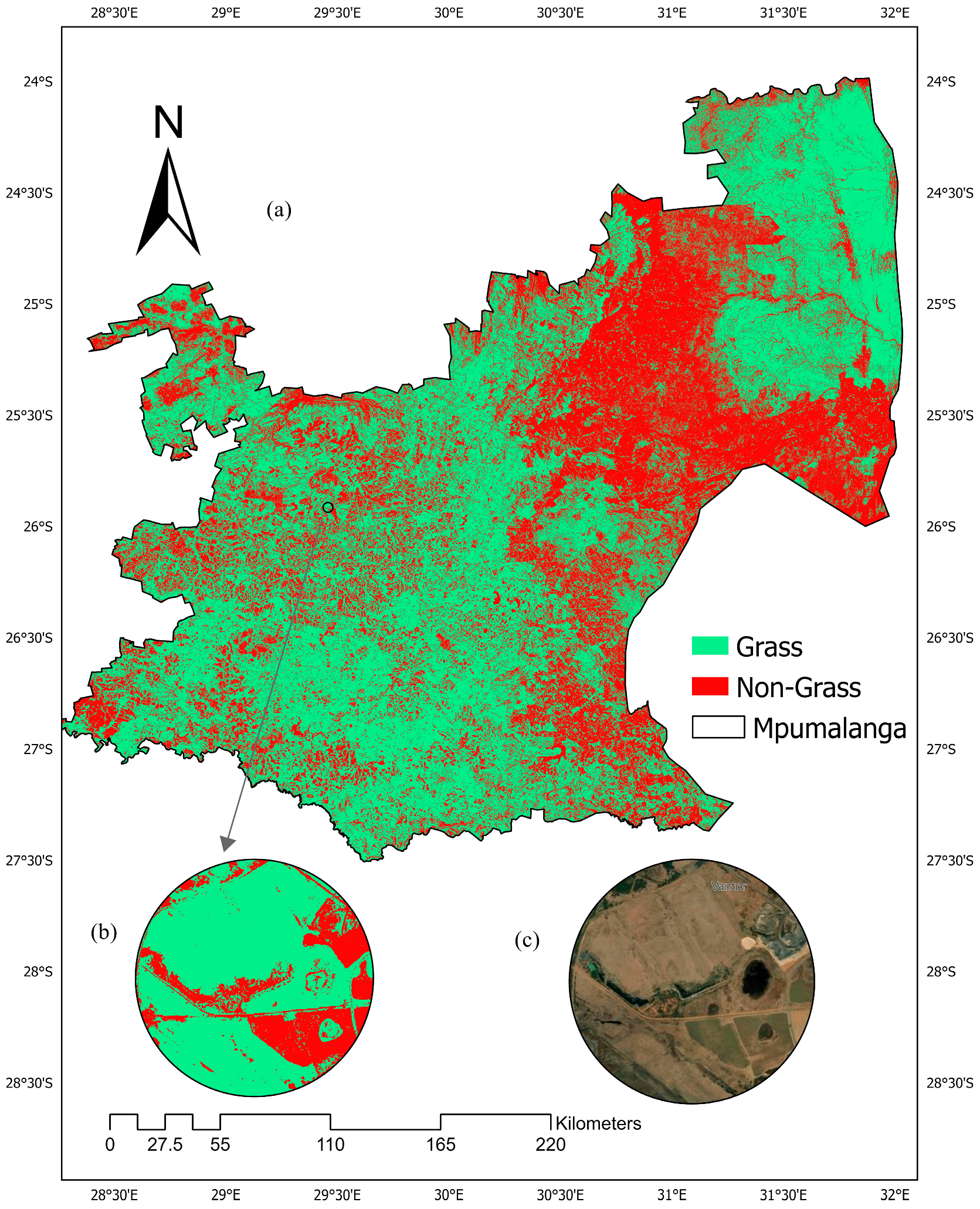
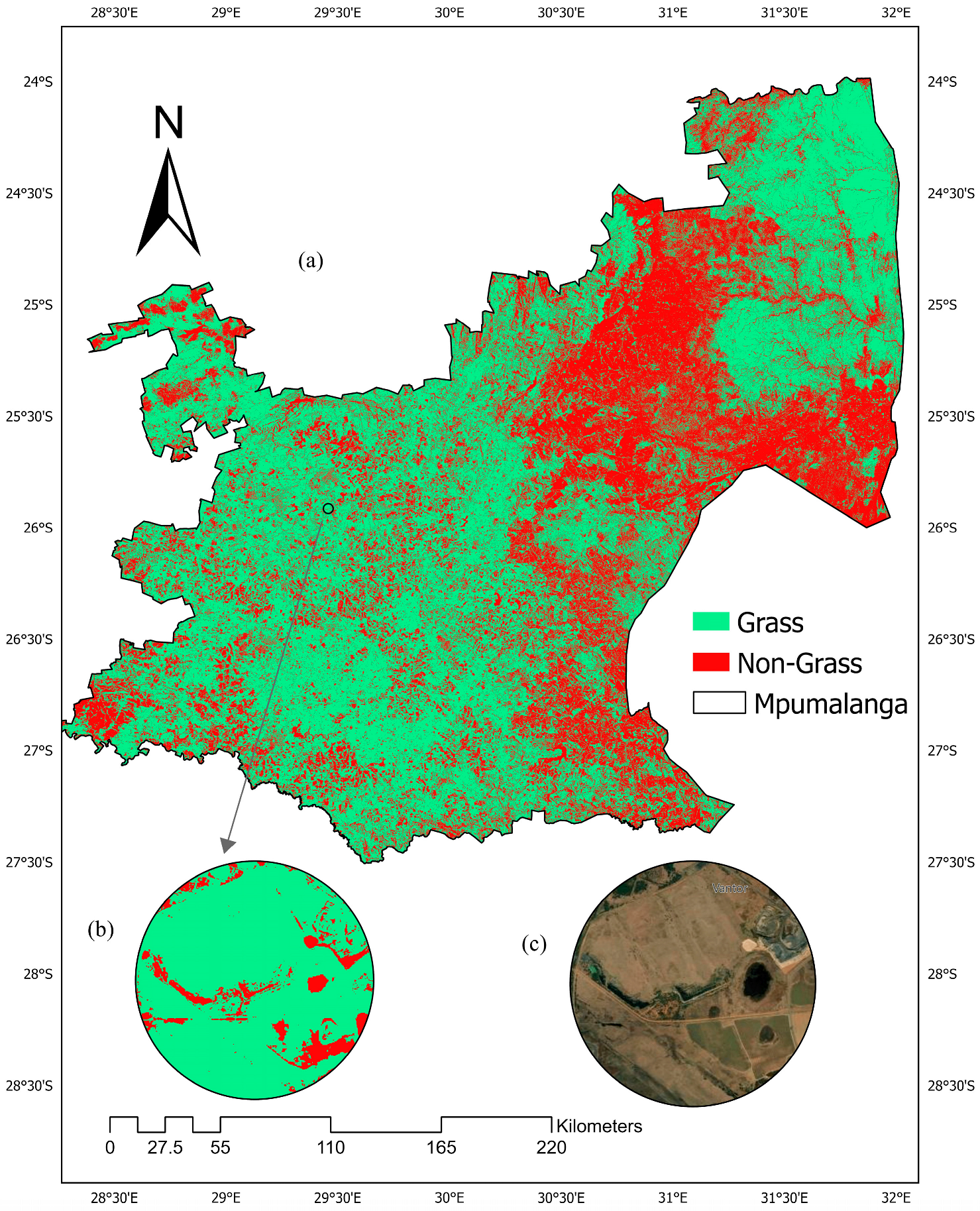
The classified maps in Figure 4 and Figure 5 illustrate the spatial distribution of grass and non-grass areas across Mpumalanga province, derived from the optimized classification model (experiment 5). As shown in the maps from both algorithms, grasslands (depicted in green) are predominantly concentrated in the central and western portions of the study area, while non-grass areas (shown in red) are more prevalent in the eastern and southeastern zones. This spatial pattern corresponds well with known vegetation gradients and land use characteristics, where grass-dominated ecosystems typically occur in lower elevations and open plains, and non-grass areas are associated with built-up, rocky, or forested environments. The minimal misclassification observed is consistent with the high precision and recall values obtained for both classes.

4. Discussion

4.1. Comparison of Classification Accuracy

This study applied RF, SVM, and 1D-CNN models to classify grasslands across Mpumalanga Province. Previous research has consistently highlighted the strong performance of these algorithms in vegetation mapping tasks [32,88]. In the present analysis, both RF and 1D-CNN demonstrated strong accuracy in binary grassland classification when integrating Sentinel-1 SAR, Sentinel-2 multispectral, and terrain derivative features. The 1D-CNN achieved an overall accuracy (OA) of 91.0%, a kappa coefficient of 0.80 with grass recall of 0.99, F1-scores of 0.93 (grass) and 0.87 (non-grass). RF surpassed this performance, attaining 97.7% OA, a kappa coefficient of 0.95 with F1-scores of 0.98 (grass) and 0.97 (non-grass), and only seven misclassifications. Although both models employed an 80/20 training validation split, the RF classifier was implemented in GEE using a random partitioning procedure, while the 1D-CNN model used a stratified train–test split in Python. Consequently, the resulting validation subsets differed slightly in sample size. By contrast, SVM yielded the lowest performance, with an OA of 80.8% and a kappa coefficient of 0.59. The model produced a recall of 91.0% for the grass class and 66.4% for the non-grass class, while precision values were 79.3% and 83.9%, respectively. Corresponding F1-scores were 84.7% for the grass class and 74.4% for the non-grass class. The 10-fold cross-validation showed that both RF and 1D-CNN models performed well, with mean accuracies of 96.9% and 91.8%, respectively, which suggests that combined Sentinel-1, Sentinel-2 and terrain features are effective for grassland and non-grass discrimination. RF achieved higher predictive accuracy than 1D-CNN by 5.7 percentage points. To determine whether this difference was statistically significant, McNemar’s test was applied to paired classification outcomes. The contingency table showed that RF correctly classified 85 samples that were misclassified by CNN, whereas CNN correctly classified only 14 samples that RF misclassified. The McNemar’s test produced a statistic of 49.49 with a p-value of 1.99 × 10⁻¹², indicating a statistically significant difference between the two models (p < 0.05).

The effectiveness of these models has been corroborated in other studies. Ref. [32] successfully employed RF to map large-scale grassland types, achieving accuracies exceeding 80%. Ref. [88] compared multiple algorithms for semi-arid grassland classification and reported that RF achieved the highest accuracy in pixel-based classification (OA = 96.32%). In object-based classification, both RF and SVM produced similarly strong results, with OA values above 97.5%, significantly outperforming other tested algorithms. Further evidence of CNN effectiveness is provided by [89], who classified plant communities in a semi-natural hay meadow in northwestern Germany using UAV imagery. Their CNN-based approach achieved accuracies up to 88% on independent test data, demonstrating the potential of CNNs for ecological and agricultural applications in high-resolution UAV datasets. Similarly, Ref. [90] compared Artificial Neural Networks (ANNs) and CNNs for predicting dry-season aboveground biomass, finding that CNNs consistently outperformed ANNs in biomass estimation.

Although both models achieved high classification accuracies, the RF model outperformed the 1D-CNN model in terms of overall accuracy, F1-score, and cross-validation performance. In addition to classification accuracy, practical considerations such as computational efficiency and model interpretability are important when selecting a classification approach. RF required lower computational resources and shorter training time and provided better interpretability through variable importance measures, making it more operationally efficient for grassland mapping applications. In contrast, the 1D-CNN model required greater computational complexity and parameter tuning despite achieving competitive performance. Furthermore, McNemar’s statistical test confirmed that the performance difference between RF and 1D-CNN was statistically significant, indicating that the superior performance of RF was not due to random variation. Additionally, RF remained highly effective for structured multi-source remote-sensing datasets.

Machine learning algorithms and deep learning algorithms exhibit distinct strengths and limitations. While RF and CNNs often demonstrate superior performance, SVM outperformed RF in other studies [91], showing the importance of evaluating algorithm suitability prior to ecosystem mapping to ensure optimal classification outcomes. Although the performance of SVM was considerably lower than that of RF and 1D-CNN in the present study, it has yielded strong results in other applications [91], particularly when dealing with relatively small training datasets and limited land use/land cover categories, where it can surpass RF. However, its performance tends to decline in large-scale LULC mapping tasks involving extensive training samples [63]. The relatively poor performance of SVM in this study may be attributed to the large and heterogeneous dataset used for training. The superior performance of RF and 1D-CNN can partly be attributed to their ability to model complex non-linear relationships between spectral, radar, and terrain variables. RF is particularly effective when dealing with high-dimensional remote sensing datasets containing correlated predictors, such as multispectral bands and derived indices.

4.2. The Impacts of Multi-Sensor Data Fusion and Classification Features on Grassland Cover Mapping

The multi-sensor fusion approach for grassland classification in Mpumalanga Province combines Sentinel-1 radar backscatter, Sentinel-2 optical bands, vegetation indices, and terrain derivatives to maximize discrimination between grassland and non-grassland vegetation. Sentinel-1 radar provides cloud-free structural information essential during the region’s summer monsoon season, capturing grass canopy architecture and surface moisture patterns that distinguish senesced grassland from bare soil. Sentinel-2 multispectral bands deliver spectral signatures for vegetation type separation while soil-adjusted indices account for bare ground exposure prevalent in savanna-grassland transition zones. Terrain features correct for topographic effects on insolation, soil stability, and moisture availability that strongly influence grass distribution patterns; this comprehensive data integration substantially outperforms single-sensor approaches typical in regional grassland mapping studies [33,85]. Additionally, Mpumalanga Province grasslands often occur in heterogeneous landscapes containing cropland, shrubs, and woodland patches. These land cover types can exhibit similar spectral signatures during the dry season, making classification challenging when relying on optical data alone.

The high classification accuracy obtained in this study is consistent with findings from other grassland and vegetation mapping studies that have applied multi-source remote sensing data. Previous research has demonstrated that the integration of radar and optical imagery significantly improves land cover classification performance compared to single-sensor approaches. For example, Ref. [85] reported that combining Sentinel-1 and Sentinel-2 data improved grassland classification accuracy due to the complementary structural and spectral information provided by radar and optical sensors. Similarly, Ref. [63] found that multispectral Sentinel-2 bands significantly enhanced vegetation discrimination in heterogeneous landscapes, achieving overall accuracies above 90% in grassland and rangeland mapping. Studies using vegetation indices have also shown improvements in vegetation detection; however, their performance is often lower than that of models using full spectral bands because indices represent simplified transformations of spectral information [92,93]. The overall accuracy of 97.7% achieved using the multi-source feature set in this study is therefore comparable to, and in some cases higher than, accuracies reported in similar studies, highlighting the effectiveness of integrating radar, optical, and terrain-derived variables for grassland classification in complex landscapes [63,85].

4.3. Comparison Between 1D-CNN and RF Model on Grass Class

The 1D-CNN model demonstrated strong performance in detecting the grass class. Out of all grass reference samples, 162 pixels were correctly classified, with only one false negative recorded. This resulted in a producer’s accuracy (recall) of 0.99, indicating that the model successfully identified most grassland areas present in the testing dataset. The high recall reflects the strong pattern-recognition capability of convolutional networks, which are effective at learning nonlinear relationships within multisource feature vectors. This behavior suggests that the 1D-CNN model strongly captured the spectral–structural signature associated with grassland cover. However, the grass class precision was lower (0.87), caused by 25 non-grass pixels incorrectly labeled as grass. These commission errors indicate a tendency of the 1D-CNN model to favor grass predictions, leading to an overestimation of grassland extent. Such behavior is common in deep learning classifiers optimized to minimize omission errors, where recall is prioritized over precision.

The RF model also performed strongly for the grass class, correctly identifying 155 grass samples, with only one grass pixel misclassified as non-grass. This resulted in a grass-class recall of 0.994, which is marginally lower than that of the 1D-CNN but still indicates near-complete detection. Importantly, RF achieved higher precision (0.969) than the 1D-CNN, meaning fewer non-grass pixels were incorrectly classified as grass. The reduced number of false positives (5 compared to 25 for 1D-CNN) indicates that the RF model was more conservative when assigning the grass label. The grass-class F1-score of 0.981 demonstrates a better balance between omission and commission errors compared to the CNN model. While RF missed a very small number of grass pixels, it compensated by producing cleaner grassland boundaries and less over-classification.

Compared with previous studies using Sentinel-2 imagery for grassland mapping, the 1D-CNN recall of 0.99 and RF F1-score of 0.981 exceed commonly reported values of 0.90–0.95 [37,94], demonstrating the effectiveness of integrating multisource features with deep learning and ensemble learning techniques. Minor misclassifications in both models may arise from spectral similarity between grasses and other herbaceous vegetation, mixed pixels, or limitations of spatial resolution, which should be considered when interpreting results. Overall, both 1D-CNN and RF provide reliable frameworks for high-accuracy grassland mapping, with model choice guided by the desired balance between detection completeness and classification precision.

4.4. Comparison Between 1D-CNN and RF Model on Non-Grass Class Performance

For the non-grass class, the 1D-CNN correctly classified 90 non-grass pixels but misclassified 25 non-grass samples as grass, resulting in a recall of 0.78. This indicates that approximately 22% of non-grass areas were omitted, primarily due to confusion with grassland features. Despite this omission error, the 1D-CNN achieved very high precision (0.99) for non-grass, meaning that most pixels predicted as non-grass were correctly labeled. This suggests that when the 1D-CNN assigns the non-grass class, it does so with high reliability. The non-grass F1-score of 0.87 indicates strong overall performance, although the lower recall highlights challenges in distinguishing non-grass surfaces that share similar spectral or structural characteristics with grassland.

The RF classifier demonstrated slightly improved performance for the non-grass class. It correctly identified 105 non-grass samples, with fewer omission errors, resulting in a recall of 0.955, higher than that of the 1D-CNN. Precision remained very high (0.991), indicating minimal commission error. The RF model therefore achieved both strong detection and reliable discrimination of non-grass areas, producing a higher non-grass F1-score (0.972) compared to 1D-CNN. The improved recall suggests that RF better differentiated non-grass surfaces such as bare soil, built-up areas, or croplands that may exhibit reflectance patterns partially overlapping with grassland. 1D-CNN is advantageous when the objective is to ensure complete identification of grassland areas, such as habitat mapping or ecological monitoring, where missing grass pixels are undesirable. RF is more suitable for land-cover inventory and area estimation tasks, where overestimation of grassland could introduce significant bias. The results indicate that while deep learning models exhibit strong detection capability, ensemble machine-learning approaches provide more consistent class balance and improved reliability for operational grassland mapping.

4.5. Limitations and Future Research

While RF and 1D-CNN demonstrated strong efficiency in mapping grassland cover across Mpumalanga Province, several limitations warrant consideration. First, the analysis relied on Sentinel-1 and Sentinel-2 imagery acquired between June and December 2024, representing a restricted temporal window. Grassland ecosystems undergo marked seasonal variability driven by phenological processes such as greening, senescence, biomass accumulation, and management activities such as grazing and harvesting. These dynamics influence spectral reflectance and radar backscatter, potentially affecting model performance under different climatic or phenological conditions. As a result, the developed models may perform differently during dry-season or early-growth periods when vegetation contrast is reduced. Future studies should incorporate multi-seasonal and multi-year datasets to capture phenological dynamics more comprehensively and improve temporal effectiveness. The integration of seasonal composites, vegetation index trajectories, and time-series deep learning approaches may further enhance generalization across diverse environmental conditions.

Classification accuracy may be affected by the spatial resolution of the input imagery. Although combining 10 m and selected 20 m Sentinel-2 bands provided useful spatial detail, mixed pixels and landscape heterogeneity can still introduce uncertainty, particularly in fragmented or transitional areas. Moreover, Sentinel-1 SAR data are inherently influenced by speckle noise and variations in soil moisture, vegetation structure, and surface roughness, which may reduce backscatter consistency despite preprocessing and filtering. Another limitation arises from the simplified binary classification scheme, which distinguishes only grassland and non-grassland. While this framework enabled robust discrimination and streamlined implementation, it oversimplifies ecological heterogeneity. Despite the high classification accuracies achieved by both RF and 1D-CNN models, potential sources of performance overestimation should be acknowledged.

Although stratified random sampling was applied to preserve class distributions between grassland and non-grassland samples, complete spatial independence between training and validation samples may not have been fully guaranteed. Spatial autocorrelation among geographically proximate samples can artificially inflate classification performance because neighboring samples often exhibit similar spectral and environmental characteristics. In addition, the use of point-based reference samples may not fully capture within-class heterogeneity across the study area. The relatively high accuracies observed in this study may also be influenced by the integration of complementary multisource predictors, including spectral, vegetation index, SAR, and terrain variables, as well as the simplified binary classification framework.

Grasslands vary in species composition, degradation status, productivity, and management conditions, and a binary approach may mask important sub-class variability. Future research should therefore explore multi-class classification strategies capable of distinguishing ecological states and management conditions. Furthermore, the training and validation datasets were derived from point samples rather than polygon-based reference data. Although point sampling is widely used, it may not fully capture spatial variability within heterogeneous pixels, especially near class boundaries. Sampling uncertainty may also result from geolocation errors, mixed pixels, and temporal mismatches between reference data and satellite imagery. While GEE facilitated efficient large-scale processing, advanced deep learning architectures cannot yet be fully trained natively within the platform, limiting model complexity compared to dedicated offline environments.

Moreover, the transferability of the developed models to other ecological regions remains uncertain. Differences in climate, vegetation composition, topography, soil characteristics, and land management practices may influence spectral and radar responses, thereby affecting generalization. Broader validation across diverse ecological contexts is needed before operational deployment. Future studies should also adopt spatial cross-validation strategies and independent validation datasets to minimize spatial dependence and strengthen robustness. Despite these limitations, this study demonstrates the strong potential of multisource remote sensing data combined with machine-learning and deep-learning approaches for accurate grassland mapping. The results highlight the effectiveness of integrating spectral, radar, terrain, and vegetation index features, providing a solid foundation for future advancements in large-scale land-cover classification and grassland monitoring systems.

5. Conclusions

This study investigated the effectiveness of multisource remote sensing data and machine-learning approaches for grassland mapping using Sentinel-1 and Sentinel-2 imagery. Five experimental feature configurations were evaluated to quantify the contribution of radar backscatter, optical spectral bands, vegetation indices, and terrain variables to classification performance. In addition, the performance of a traditional ensemble classifier (RF) was compared with a deep learning approach (1D-CNN). The experimental results demonstrated that classification accuracy varied substantially depending on the type and number of input features. Among the individual feature groups, terrain variables produced the lowest accuracy, confirming that topographic information alone is insufficient for reliable grassland discrimination. Radar backscatter improved performance relative to terrain data but remained limited when used independently. Vegetation indices provided moderate improvement by enhancing vegetation characteristics, while multispectral Sentinel-2 bands yielded substantially higher accuracy, highlighting the importance of spectral information in land-cover classification. The highest performance was achieved when all feature groups were integrated. The combined dataset, consisting of radar, spectral, vegetation index, and terrain features, resulted in an overall accuracy of 97.74%, representing a 12.4% improvement over the weakest experiment. These findings confirm the strong complementary nature of multisource data and emphasize that feature diversity plays a critical role in improving grassland classification accuracy.

References

1. Briske, D.D. Conservation Benefits of Rangeland Practices: Assessment, Recommendations, and Knowledge Gaps; United States Department of Agriculture, Natural Resources Conservation Service: Washington, DC, USA, 2007.
2. Bengtsson, J.; Bullock, J.M.; Egoh, B.; Everson, C.; Everson, T.; O’Connor, T.; O’Farrell, P.; Smith, H.G.; Lindborg, R. Grasslands-more important for ecosystem services than you might think. Ecosphere 2019, 10, e02582. [Google Scholar] [CrossRef]
3. Latham, J.; Cumani, R.; Rosati, I.; Bloise, M. Global Land Cover SHARE (GLC-SHARE) Database Beta-Release Version 1.0—2014; FAO: Rome, Italy, 2014; p. 29. [Google Scholar]
4. Bardgett, R.D.; Bullock, J.M.; Lavorel, S.; Upadhyaya, S.; Bondeau, A.; Chenu, C.; Chappell, A.; Christie, A.; Cruse, R.; Delgado-Baquerizo, M.; et al. Combatting global grassland degradation. Nat. Rev. Earth Environ. 2021, 2, 720–735. [Google Scholar] [CrossRef]
5. Mousavi, M.; Biney, J.K.M.; Kishchuk, B.; Youssef, A.; Cordeiro, M.R.; Friesen, G.; Cattani, D.; Namous, M.; Badreldin, N. A hierarchical machine learning-based strategy for mapping grassland. Remote Sens. 2024, 16, 4730. [Google Scholar] [CrossRef]
6. Boval, M.; Dixon, R.M. The importance of grasslands for animal production and other functions: A review on management and methodological progress in the tropics. Animal 2012, 6, 748–762. [Google Scholar] [CrossRef]
7. Gibson, D.J. Grasses and Grassland Ecology; Oxford University Press: Oxford, UK, 2009. [Google Scholar]
8. McInnes, W.S.; Smith, B.; McDermid, G.J. Discriminating native and nonnative grasses in the dry mixedgrass prairie with MODIS NDVI time series. IEEE J. Sel. Top. Appl. Earth Obs. Remote Sens. 2015, 8, 1395–1403. [Google Scholar] [CrossRef]
9. Slooten, E.; Jordaan, E.; White, J.D.; Archibald, S.; Siebert, F. South African grasslands and ploughing: Outlook for agricultural expansion in Africa. S. Afr. J. Sci. 2023, 119, 1–4. Available online: https://www.scielo.org.za/scielo.php?pid=S0038-23532023000500005&script=sci_arttext (accessed on 15 May 2026). [CrossRef]
10. Carbutt, C.; Tau, M.; Stephens, A.; Escott, B. The conservation status of temperate grasslands in southern Africa. Grassroots 2011, 11, 17–23. [Google Scholar]
11. BirdLife, S.A. South African Grassland Biome. Giving Conservation Wings. Lesson Plan 2; BirdLife South Africa: Johannesburg, South Africa, 2019. [Google Scholar]
12. Carbutt, C.; Kirkman, K. Ecological grassland restoration—A South African perspective. Land 2022, 11, 575. [Google Scholar] [CrossRef]
13. Zhao, Y.; Wang, J.; Zhang, G.; Liu, L.; Yang, J.; Wu, X.; Biradar, C.; Dong, J.; Xiao, X. Divergent trends in grassland degradation and desertification under land use and climate change in Central Asia from 2000 to 2020. Ecol. Indic. 2023, 154, 110737. [Google Scholar] [CrossRef]
14. Encabo, J.B.M.; Cordeiro, M.R. Leveraging remote sensing products to estimate grassland productivity in the Canadian Prairies. Anim. Sci. Cases 2024, ascs20240005. [Google Scholar] [CrossRef]
15. Ali, I.; Cawkwell, F.; Dwyer, E.; Barrett, B.; Green, S. Satellite remote sensing of grasslands: From observation to management. J. Plant Ecol. 2016, 9, 649–671. [Google Scholar] [CrossRef]
16. Wang, Z.; Ma, Y.; Zhang, Y.; Shang, J. Review of remote sensing applications in grassland monitoring. Remote Sens. 2022, 14, 2903. [Google Scholar] [CrossRef]
17. Tandzi, N.L.; Mutengwa, C.S. Exploitation of the indigenous knowledge in crop improvement using remote sensing in sub-Saharan Africa. Int. J. Remote Sens. 2019, 40, 9123–9145. [Google Scholar]
18. Dong, J.; Xiao, X.; Menarguez, M.A.; Zhang, G.; Qin, Y.; Thau, D.; Biradar, C.; Moore, B. Mapping paddy rice planting area in northeastern Asia with Landsat 8 images, phenology-based algorithm and Google Earth Engine. Remote Sens. Environ. 2016, 185, 142–154. [Google Scholar] [CrossRef] [PubMed]
19. Kumar, L.; Mutanga, O. Google Earth Engine applications since inception: Usage, trends, and potential. Remote Sen. 2018, 10, 1509. [Google Scholar] [CrossRef]
20. Mutanga, O.; Kumar, L. Google Earth Engine applications. Remote Sens. 2019, 11, 591. [Google Scholar] [CrossRef]
21. Gorelick, N.; Hancher, M.; Dixon, M.; Ilyushchenko, S.; Thau, D.; Moore, R. Google Earth Engine: Planetary-scale geospatial analysis for everyone. Remote Sens. Environ. 2017, 202, 18–27. [Google Scholar] [CrossRef]
22. Zurqani, H.A.; Post, C.J.; Mikhailova, E.A.; Schlautman, M.A.; Sharp, J.L. Geospatial analysis of land use change in the Savannah River Basin using Google Earth Engine. Int. J. Appl. Earth Obs. Geoinf. 2018, 69, 175–185. [Google Scholar] [CrossRef]
23. Mashaba Munghemezulu, Z.; Nduku, L.; Munghemezulu, C.; Chirima, G.J. Research progress in the application of Google Earth Engine for grasslands based on a bibliometric analysis. Grasses 2024, 3, 69–83. [Google Scholar] [CrossRef]
24. Tsai, Y.H.; Stow, D.; Chen, H.L.; Lewison, R.; An, L.; Shi, L. Mapping vegetation and land use types in Fanjingshan National Nature Reserve using Google Earth Engine. Remote Sens. 2018, 10, 927. [Google Scholar] [CrossRef]
25. Traganos, D.; Aggarwal, B.; Poursanidis, D.; Topouzelis, K.; Chrysoulakis, N.; Reinartz, P. Towards global-scale seagrass mapping and monitoring using Sentinel 2 on Google Earth Engine: The case study of the Aegean and Ionian seas. Remote Sens. 2018, 10, 1227. [Google Scholar] [CrossRef]
26. Ji, R.; Tan, K.; Wang, X.; Pan, C.; Xin, L. Spatiotemporal monitoring of a grassland ecosystem and its net primary production using Google Earth Engine: A case study of Inner Mongolia from 2000 to 2020. Remote Sens. 2021, 13, 4480. [Google Scholar] [CrossRef]
27. Poortinga, A.; Clinton, N.; Saah, D.; Cutter, P.; Chishtie, F.; Markert, K.N.; Anderson, E.R.; Troy, A.; Fenn, M.; Tran, L.H.; et al. An operational before after control impact (BACI) designed platform for vegetation monitoring at planetary scale. Remote Sens. 2018, 10, 760. [Google Scholar] [CrossRef]
28. Reza Pahlefi, M.; Danoedoro, P.; Kamal, M. The utilisation of Sentinel 2A images and Google Earth Engine for monitoring tropical savannah grassland. Geocarto Int. 2022, 37, 5400–5414. [Google Scholar] [CrossRef]
29. Shao, Z.; Ahmad, M.N.; Javed, A. Comparison of random forest and XGBoost classifiers using integrated optical and SAR features for mapping urban impervious surface. Remote Sens. 2024, 16, 665. [Google Scholar] [CrossRef]
30. Rapinel, S.; Mony, C.; Lecoq, L.; Clément, B.; Thomas, A.; Hubert Moy, L. Evaluation of Sentinel 2 time series for mapping floodplain grassland plant communities. Remote Sens. Environ. 2019, 223, 115–129. [Google Scholar] [CrossRef]
31. Zhao, C.; Qin, C.Z. Identifying mangrove distribution using remote sensing. Int. J. Appl. Earth Obs. Geoinf. 2022, 108, 102750. [Google Scholar]
32. Yu, H.; Zhu, L.; Chen, Y.; Yue, Z.; Zhu, Y. Improving grassland classification accuracy using optimal spectral phenological topographic features in combination with machine learning algorithm. Ecol. Indic. 2024, 158, 111392. [Google Scholar] [CrossRef]
33. Li, S.; Tian, S. A deep feature fusion method for complex ground object classification in the land cover ecosystem. Land 2023, 12, 1022. [Google Scholar] [CrossRef]
34. Lin, X.; Chen, J.; Wu, T.; Yi, S.; Chen, J.; Han, X. Time series simulation of alpine grassland cover using transferable stacking deep learning and multisource remote sensing data in Google Earth Engine. Int. J. Appl. Earth Obs. Geoinf. 2024, 131, 103964. [Google Scholar]
35. Ma, H.; Liang, S. Development of the GLASS 250 m leaf area index product using LSTM. Remote Sens. Environ. 2022, 273, 112985. [Google Scholar] [CrossRef]
36. Chen, J.; Chen, Z.; Huang, R.; You, H.; Han, X.; Yue, T.; Zhou, G. The effects of spatial resolution and resampling on the classification accuracy of wetland vegetation species and ground objects: A study based on high spatial resolution UAV images. Drones 2023, 7, 61. [Google Scholar] [CrossRef]
37. Song, Y.; Zhang, Z.; Baghbaderani, R.K.; Wang, F.; Qu, Y.; Stuttsy, C.; Qi, H. Land cover classification for satellite images through 1D CNN. In WHISPERS; IEEE: Amsterdam, The Netherlands, 2019; pp. 1–5. [Google Scholar]
38. Bai, T.; Wang, L.; Yin, D.; Sun, K.; Chen, Y.; Li, W.; Li, D. Deep learning for change detection in remote sensing: A review. Geo. Spat. Inf. Sci. 2023, 26, 262–288. [Google Scholar] [CrossRef]
39. Zhu, X.X.; Tuia, D.; Mou, L.; Xia, G.S.; Zhang, L.; Xu, F.; Fraundorfer, F. Deep learning in remote sensing: A comprehensive review. IEEE J. Sel. Top. Appl. Earth Obs. Remote Sens. 2017, 5, 8–36. [Google Scholar]
40. Ali, I.; Cawkwell, F.; Dwyer, E.; Green, S. Modeling managed grassland biomass estimation by using multitemporal remote sensing data—A machine learning approach. IEEE J. Sel. Top. Appl. Earth Obs. Remote Sens. 2016, 10, 3254–3264. [Google Scholar] [CrossRef]
41. Wu, C.; Shen, H.; Shen, A.; Deng, J.; Gan, M.; Zhu, J.; Xu, H.; Wang, K. Comparison of machine learning methods for above ground biomass estimation based on Landsat imagery. J. Appl. Remote Sens. 2016, 10, 035010. [Google Scholar] [CrossRef]
42. Ding, F.; Li, C.; Zhai, W.; Fei, S.; Cheng, Q.; Chen, Z. Estimation of nitrogen content in winter wheat based on multi-source data fusion and machine learning. Agriculture 2022, 12, 1752. [Google Scholar] [CrossRef]
43. Sun, C.; Bian, Y.; Zhou, T.; Pan, J. Using of multi-source and multi temporal remote sensing data improves crop type mapping in the subtropical agriculture region. Sensors 2019, 19, 2401. [Google Scholar] [CrossRef] [PubMed]
44. Wang, W.; Ma, Q.; Huang, J.; Feng, Q.; Zhao, Y.; Guo, H.; Chen, B.; Li, C.; Zhang, Y. Remote sensing monitoring of grasslands based on adaptive feature fusion with multi source data. Remote Sens. 2022, 14, 750. [Google Scholar] [CrossRef]
45. Zhou, Y.; Liu, T.; Batelaan, O.; Duan, L.; Wang, Y.; Li, X.; Li, M. Spatiotemporal fusion of multi-source remote sensing data for estimating aboveground biomass of grassland. Ecol. Indic. 2023, 146, 109892. [Google Scholar] [CrossRef]
46. Badreldin, N.; Uuemaa, E.; Pärtel, M. Identifying native grasslands and key phenological stages using multiple satellite data sources. Remote Sens. 2021, 13, 3012. [Google Scholar]
47. Wang, Y.; Wu, G.; Deng, L.; Tang, Z.; Wang, K.; Sun, W.; Shangguan, Z. Prediction of aboveground grassland biomass on the Loess Plateau, China, using a random forest algorithm. Sci. Rep. 2017, 7, 6940. [Google Scholar] [CrossRef] [PubMed]
48. Zeng, N.; Ren, X.; He, H.; Zhang, L.; Zhao, D.; Ge, R.; Li, P.; Niu, Z. Estimating grassland aboveground biomass on the Tibetan Plateau using a random forest algorithm. Ecol. Indic. 2019, 102, 479–487. [Google Scholar] [CrossRef]
49. Basavegowda, D.H.; Schleip, I.; Mosebach, P.; Weltzien, C. Deep learning based detection of indicator species for monitoring biodiversity in semi natural grasslands. Environ. Sci. Ecol. Technol. 2024, 21, 100419. [Google Scholar] [CrossRef]
50. Kattenborn, T.; Eichel, J.; Fassnacht, F.E. Convolutional Neural Networks enable efficient, accurate and fine grained segmentation of plant species and communities from high resolution UAV imagery. Sci. Rep. 2019, 9, 17656. [Google Scholar] [CrossRef]
51. Alirezazadeh, P.; Schirrmann, M.; Stolzenburg, F. Improving deep learning based plant disease classification with attention mechanism. Gesunde Pflanze 2023, 75, 49–59. [Google Scholar] [CrossRef]
52. Wäldchen, J.; Rzanny, M.; Seeland, M.; Mäder, P. Automated plant species identification—Trends and future directions. PLoS Comput. Biol. 2018, 14, e1005993. [Google Scholar] [CrossRef]
53. Valente, J.; Doldersum, M.; Roers, C.; Kooistra, L. Detecting Rumex obtusifolius weed plants in grasslands from UAV RGB imagery using deep learning. ISPRS Ann. Photogramm. Remote Sens. Spat. Inf. Sci. 2019, 4, 179–185. [Google Scholar] [CrossRef]
54. Fourie, L.; Rouget, M.; Lötter, M. Landscape connectivity of the grassland biome in Mpumalanga, South Africa. Austral Ecol. 2015, 40, 67–76. [Google Scholar] [CrossRef]
55. Ferrar, A.A.; Lötter, M.C. Mpumalanga Biodiversity Conservation Plan Handbook; Mpumalanga Tourism & Parks Agency: Nelspruit, South Africa, 2007.
56. Louw, J.H. A site growth study of Eucalyptus grandis in the Mpumalanga escarpment area. South. Afr. For. J. 1997, 180, 1–14. [Google Scholar]
57. van der Merwe, J.P.; Wang, T.; Clarke, C.; Mansfield, S.D. Predicting temperature and rainfall for plantation forestry in Mpumalanga, South Africa. Agric. For. Meteorol. 2023, 329, 109275. [Google Scholar] [CrossRef]
58. Zhang, W.; Brandt, M.; Wang, Q.; Prishchepov, A.V.; Tucker, C.J.; Li, Y.; Lyu, H.; Fensholt, R. From woody cover to woody canopies: How Sentinel 1 and Sentinel 2 data advance the mapping of woody plants in savannas. Remote Sens. Environ. 2019, 234, 111465. [Google Scholar] [CrossRef]
59. Praticò, S.; Solano, F.; Di Fazio, S.; Modica, G. Machine learning classification of Mediterranean forest habitats in Google Earth Engine based on seasonal Sentinel 2 time series and input image composition optimisation. Remote Sens. 2021, 13, 586. [Google Scholar] [CrossRef]
60. Wang, Q.; Jin, T.; Li, J.; Chang, X.; Li, Y.; Zhu, Y. Modeling and Assessment of Vegetation Water Content on Soil Moisture Retrieval via the Synergistic Use of Sentinel-1 and Sentinel-2. Earth Space Sci. 2022, 9, e2021EA002063. [Google Scholar] [CrossRef]
61. Vreugdenhil, M.; Wagner, W.; Bauer-Marschallinger, B.; Pfeil, I.; Teubner, I.; Rüdiger, C.; Strauss, P. Sensitivity of Sentinel-1 Backscatter to Vegetation Dynamics: An Austrian Case Study. Remote Sens. 2018, 10, 1396. [Google Scholar] [CrossRef]
62. Inglada, J.; Michel, J.; Hagolle, O. Assessment of the usefulness of spectral bands for the next generation of Sentinel 2 satellites. Remote Sens. 2022, 14, 2503. [Google Scholar] [CrossRef]
63. Feng, S.; Li, W.; Xu, J.; Liang, T.; Ma, X.; Wang, W.; Yu, H. Land use/land cover mapping based on Google Earth Engine for monitoring ecosystem changes. Remote Sens. 2022, 14, 5361. [Google Scholar] [CrossRef]
64. Verde, N.; Kokkoris, I.P.; Georgiadis, C.; Kaimaris, D.; Dimopoulos, P.; Mitsopoulos, I.; Mallinis, G. National scale land cover classification using Copernicus EO data and Google Earth Engine. Remote Sens. 2020, 12, 3303. [Google Scholar] [CrossRef]
65. Parente, L.; Sloat, L.; Mesquita, V.; Consoli, D.; Stanimirova, R.; Hengl, T.; Bonannella, C.; Teles, N.; Wheeler, I.; Hunter, M.; et al. Annual 30 m maps of global grassland class and extent (2000–2022). Sci. Data 2024, 11, 1303. [Google Scholar] [CrossRef]
66. Zhao, Y.; Zhu, W.; Wei, P.; Fang, P.; Zhang, X.; Yan, N.; Liu, W.; Zhao, H.; Wu, Q. Classification of Zambian grasslands using random forest feature importance selection during the optimal phenological period. Ecol. Indic. 2022, 135, 108529. [Google Scholar] [CrossRef]
67. Shi, Y.; Gao, J.; Brierley, G.; Li, X.; Perry, G.L.W.; Xu, T. Improving the accuracy of models to map alpine grassland biomass using Google Earth Engine. Grass Forage Sci. 2023, 78, 237–253. [Google Scholar] [CrossRef]
68. Li, X.; Chen, W.; Cheng, X.; Wang, L. A comparison of machine learning algorithms for mapping of complex landscapes. Remote Sens. 2016, 8, 514. [Google Scholar] [CrossRef]
69. Amini, S.; Saber, M.; Rabiei Dastjerdi, H.; Homayouni, S. Urban land use and land cover change analysis using random forest classification of Landsat time series. Remote Sens. 2022, 14, 2654. [Google Scholar] [CrossRef]
70. Phan, T.N.; Kuch, V.; Lehnert, L.W. Land cover classification using Google Earth Engine and random forest classifier. Remote Sens. 2020, 12, 2411. [Google Scholar] [CrossRef]
71. Liu, H.Q.; Huete, A. A feedback-based modification of the NDVI to minimize canopy background and atmospheric noises. Remote Sens. Environ. 1995, 54, 204–214. [Google Scholar] [CrossRef]
72. Huete, A.R. A soil adjusted vegetation index (SAVI). Remote Sens. Environ. 1988, 25, 295–309. [Google Scholar] [CrossRef]
73. Huete, A.; Didan, K.; Miura, T.; Rodriguez, E.P.; Gao, X.; Ferreira, L.G. Overview of the radiometric and biophysical performance of the MODIS vegetation indices. Remote Sens. Environ. 2002, 83, 195–213. [Google Scholar] [CrossRef]
74. Li, F.; Zhu, Y.; Cao, Q.; Cheng, T.; Tian, Y. Estimating leaf nitrogen concentration from hyperspectral data using vegetation indices. Precis. Agric. 2014, 15, 511–527. [Google Scholar]
75. Wu, C.; Niu, Z.; Gao, S. Satellite derived chlorophyll index for estimating light use efficiency. Ecol. Indic. 2012, 14, 66–73. [Google Scholar] [CrossRef]
76. Ghorbanian, A.; Zaghian, S.; Asiyabi, R.M.; Amani, M.; Mohammadzadeh, A.; Jamali, S. Mangrove ecosystem mapping using sentinel-1 and sentinel-2 satellite images and random forest algorithm in google earth engine. Remote Sens. 2021, 13, 2565. [Google Scholar] [CrossRef]
77. Hu, N.; Liu, Y.; Ge, X.; Dong, X.; Wang, H.; Long, Y.; Wang, L. Mapping the invasive species Stellera chamaejasme in alpine grasslands using ecological clustering, spectral separability and image classification. Agronomy 2023, 13, 593. [Google Scholar] [CrossRef]
78. Ma, L.; Liu, Y.; Zhang, X.; Ye, Y.; Yin, G.; Johnson, B.A. Deep learning in remote sensing applications: A meta-analysis and review. ISPRS J. Photogramm. Remote Sens. 2019, 152, 166–177. [Google Scholar] [CrossRef]
79. Liu, J.; Wang, T.; Skidmore, A.; Sun, Y.; Jia, P.; Zhang, K. Integrated 1D, 2D, and 3D CNNs enable robust land cover classification. Remote Sens. 2023, 15, 4797. [Google Scholar] [CrossRef]
80. Fan, X.; Chen, L.; Xu, X.; Yan, C.; Fan, J.; Li, X. Land cover classification of remote sensing images based on hierarchical convolutional recurrent neural network. Forests 2023, 14, 1881. [Google Scholar] [CrossRef]
81. Zhang, H.K.; Roy, D.P.; Luo, D. Large area land cover classification using 1D CNN. Remote Sens. Environ. 2023, 295, 113653. [Google Scholar] [CrossRef]
82. Hu, X.; Yang, W.; Wen, H.; Liu, Y.; Peng, Y. A lightweight 1 D convolution augmented transformer with metric learning for hyperspectral image classification. Sensors 2021, 21, 1751. [Google Scholar] [PubMed]
83. Pullanagari, R.R.; Dehghan Shoar, M.; Yule, I.J.; Bhatia, N. Field spectroscopy of canopy nitrogen concentration using CNN. Remote Sens. Environ. 2021, 257, 112353. [Google Scholar]
84. Pu, Y.; Nixon, A.; Prieto, B.; Guo, X. Identifying native grasslands and phenological stages using Sentinel 2 data and deep learning. Int. J. Appl. Earth Obs. Geoinf. 2025, 140, 104619. [Google Scholar]
85. Li, S.; Guo, P.; Sun, F.; Zhu, J.; Cao, X.; Dong, X.; Lu, Q. Mapping dryland ecosystems using Google Earth Engine and Random Forest: A case study of an ecologically critical area in northern China. Land 2024, 13, 845. [Google Scholar] [CrossRef]
86. Foody, G.M. Status of land cover classification accuracy assessment. Remote Sens. Environ. 2002, 80, 185–201. [Google Scholar] [CrossRef]
87. Alem, A.; Kumar, S. Deep Learning Models Performance Evaluations for Remote Sensed Image Classification. IEEE Access 2022, 10, 111784–111793. [Google Scholar] [CrossRef]
88. Wu, N.; Crusiol, L.G.T.; Liu, G.; Wuyun, D.; Han, G. Comparing machine learning algorithms for grassland classification. Remote Sens. 2023, 15, 750. [Google Scholar] [CrossRef]
89. Pöttker, M.; Kiehl, K.; Jarmer, T.; Trautz, D. Convolutional neural network maps plant communities using UAV imagery. Remote Sens. 2023, 15, 1945. [Google Scholar] [CrossRef]
90. Vawda, M.I.; Lottering, R.; Mutanga, O.; Peerbhay, K.; Sibanda, M. Comparing ANN and CNN for estimating dry season aboveground grass biomass. Sustainability 2024, 16, 1051. [Google Scholar] [CrossRef]
91. Praveen, B.; Mustak, S.; Sharma, P. Assessing the transferability of machine learning algorithms for agricultural land use mapping. ISPRS Int. Arch. Photogramm. Remote Sens. Spat. Inf. Sci. 2019, 42, 585–592. [Google Scholar]
92. Darra, N.; Espejo Garcia, B.; Psiroukis, V.; Psomiadis, E.; Fountas, S. Spectral bands vs. vegetation indices: An AutoML approach for processing tomato yield predictions based on Sentinel 2 imagery. Smart Agric. Technol. 2025, 10, 100805. [Google Scholar] [CrossRef]
93. Karakacan Kuzucu, A.; Bektas Balcik, F. Testing the potential of vegetation indices for land use/cover classification using high resolution data. ISPRS Ann. Photogramm. Remote Sens. Spat. Inf. Sci. 2017, 4, 279–283. [Google Scholar] [CrossRef]
94. Wambugu, N.; Chen, Y.; Xiao, Z.; Wei, M.; Bello, S.A.; Junior, J.M.; Li, J. A hybrid deep convolutional neural network for land cover classification. Int. J. Appl. Earth Obs. Geoinf. 2021, 103, 102515. [Google Scholar] [CrossRef]
Figure 1. Map of Mpumalanga province, South Africa, showing different land cover classes.
Land 15 01215 g001
Figure 2. Flow diagram of the classification of grassland.
Land 15 01215 g002
Figure 3. Importance scores for the features used in classification.
Land 15 01215 g003
Figure 4. (a) Land-cover classification results produced using RF for the study area; (b,c) show land-cover categories and satellite images of the western part of Mpumalanga, respectively.
Land 15 01215 g004
Figure 5. (a) Land-cover classification results produced using the 1D-CNN model for the study area; (b,c) show land-cover categories and satellite images of the western part of Mpumalanga, respectively.
Land 15 01215 g005