Impact of Landscape Pattern on Habitat Quality in Karst Areas of Guizhou Province, China, and Analysis of Its Driving Factors

Abstract

Understanding how landscape patterns affect habitat quality in fragile karst regions is critical for biodiversity conservation, yet the driving mechanisms remain poorly understood, particularly regarding karst geomorphic heterogeneity. Taking Guizhou Province, a typical karst area of southwestern China, this study integrated land-use and natural geographic data (DEM, karst landforms, soil types, slope, soil thickness, vegetation cover, bedrock exposure, and rocky desertification) from 2000 to 2020. We quantified landscape pattern indices and habitat quality using Fragstats and InVEST, then explored spatial relationships via bivariate spatial autocorrelation and geographically weighted regression (GWR). Results show that land-use intensity increased and landscape structure stabilized, while fragmentation slightly decreased, but connectivity weakened. Habitat quality declined 4.4% over two decades. Globally, habitat quality was positively correlated with aggregation, cohesion, contagion, and largest patch index, and negatively correlated with shape complexity, patch density, diversity, and splitting indices. Locally, six karst zones exhibited distinct clustering patterns, revealing nonlinear interactions between natural vulnerability (e.g., bedrock exposure, thin soil) and human activities. After 2010, the dominant driver shifted from natural conditions to human–land interactions, with human activities contributing approximately 60% of habitat quality degradation. These findings provide a quantitative, spatially explicit basis for ecological zoning and differentiated policy making in Guizhou and similar fragile regions.

1. Introduction

Ecosystem services are the necessary resources and environments that ecosystems provide for human survival [1], with a focus on how biomes, biospheres, and ecosystems respond to natural and anthropogenic global changes [2]. Human-induced land-use/land-cover (LULC) change is a major driver of ecosystem service changes [3,4]. Consequently, regional ecosystem degradation and habitat quality (HQ) loss continue to occur [5,6]. Guizhou Province is a typical karst region with a fragile ecological environment. The province serves as an important ecological security barrier for the upper reaches of the Yangtze and Pearl Rivers. In 2016, Guizhou was included in China’s first batch of national ecological civilization pilot zones, and in 2022, it was designated as a pioneer zone for ecological civilization construction [7,8]. There is a clear correlation between HQ and LULC changes. The landscape pattern index (LSPI) can effectively describe LULC characteristics and provide targeted strategies for regional ecological management [9]. However, Guizhou contains areas with varying degrees of karst development, and existing studies lack a partitioned analysis of the driving mechanisms behind LSPI and HQ changes. Therefore, exploring the effects of LSPI changes on HQ and analyzing the underlying mechanisms across these areas is crucial for ecological conservation and policy formulation.

Habitat quality is a key indicator of regional biodiversity, reflecting the ability of ecosystems to sustain individuals and populations [10,11]. Current HQ assessments commonly use multiple indices, including the habitat quality index, vegetation cover index, water network density index, land stress index, and pollution loading index [12]. Among these, the InVEST model is widely used because it directly quantifies HQ [13,14]. Previous studies have analyzed HQ evolution at the regional, urban, watershed, and economic-belt scales and have proposed landscape plans for biodiversity conservation [15,16]. Similar correlations between land-use change and HQ have also been reported in other karst regions worldwide, such as the Mediterranean karst and Southeast Asian karst [17,18]. However, most of those studies treated karst areas as homogeneous units and did not account for geomorphic heterogeneity or spatial non-stationarity. Critically, this gap also limits the development of targeted biodiversity conservation and ecosystem protection policies.

Changes in landscape patterns have direct and indirect effects on ecosystem services, and different services respond differently [19,20]. LSPI is an important tool for quantitatively characterizing landscape composition, structure, diversity, spatial configuration, and shape complexity [21]. LSPI affects HQ by influencing regional climatic and hydrological conditions, as well as material exchange and the flow of ecological elements [22,23]. Most previous studies have relied on correlation analysis and geodetector models to examine the influence of single LSPI types on HQ at regional or watershed scales [23,24,25]. A key limitation of these approaches is that they are global in nature and cannot account for potential spatial non-stationarity in the LSPI–HQ relationship across different locations. Moreover, the relationship between LSPI and HQ remains insufficiently characterized. Previous studies have confirmed the growing dominance of anthropogenic drivers in karst regions [26,27]; however, their influence on the LSPI–HQ relationship across different karst geomorphic units remains largely unexplored. Methodologically, differential weighting of factors within attribution frameworks has also been established in previous studies [21,28], further supporting the feasibility of a period-specific weighting approach. Importantly, Guizhou Province contains areas with varying degrees of karst development —for example, non-karst areas, karst trough valleys, karst plateaus, peak-cluster depressions, faulted basins, and karst canyons [29]—and it remains unclear whether the LSPI–HQ relationship varies systematically with the degree of karst development. This karst geomorphic heterogeneity is a key source of spatial non-stationarity that must be explicitly addressed. Specifically, three knowledge gaps remain: (i) no study has partitioned Guizhou into distinct karst geomorphic units to examine LSPI–HQ relationships; (ii) the current status of HQ in areas with different degrees of karst development remains unassessed; (iii) it is unclear whether the LSPI–HQ relationship varies systematically with karst development degree, let alone the underlying nonlinear interplay of natural and anthropogenic drivers.

A unique contribution of this study is the adoption of a six-zone classification of Guizhou (non-karst, karst trough valley, karst plateau, peak-cluster depression, faulted basin, and karst canyon), which follows the national karst geomorphic zoning framework [29,30]. This zonation allows us to explicitly link geomorphic heterogeneity to HQ responses—a level of detail absent in previous work. Given the identified knowledge gaps and the unique geomorphic heterogeneity of Guizhou’s karst landscape, the overarching purpose of this study is to systematically unravel the intrinsic mechanisms through which landscape pattern changes affect habitat quality across different karst development zones. Unlike previous studies that treat karst areas as homogeneous entities or rely on global correlation analyses, our research is designed to move beyond simple descriptions of spatiotemporal changes, aiming instead to provide a mechanistic understanding of how landscape fragmentation and connectivity interact with both natural vulnerability and human activities to jointly drive habitat quality dynamics. The core contributions we anticipate are threefold: (1) to offer a spatially explicit, zonation-based diagnostic of habitat quality status that can inform targeted ecological restoration; (2) to disentangle the nonlinear interplay between natural and anthropogenic drivers, particularly the post-2010 shift toward human-dominated forcing; (3) to provide a quantitative, policy-relevant basis for differentiated ecological management in Guizhou and other fragile karst regions worldwide. To fulfill this overarching purpose, we have formulated three sequential and mutually reinforcing objectives: (1) to characterize the spatiotemporal evolution of landscape patterns and habitat quality from 2000 to 2020; (2) to reveal the spatial non-stationarity in the landscape pattern–habitat quality relationship across different karst zones using bivariate spatial autocorrelation and geographically weighted regression; (3) to identify the shifting contributions of natural and anthropogenic drivers, with particular attention to the critical turning point around 2010.

The remainder of this paper is organized as follows. Section 2 describes the study area, data sources, and research methods. Section 3 presents the empirical results. Section 4 provides a comprehensive discussion of the findings, proposes policy recommendations, and acknowledges the study’s limitations. Finally, Section 5 summarizes the main conclusions, highlights the key innovations of this work, and outlines directions for future research.

2. Materials and Methods

2.1. Study Area

Guizhou Province is located in the karst region of Southwest China. The exposed karst area accounts for 61.92% of the province’s total land area, and when covered and shallow-buried karst are included, the total karst distribution area reaches approximately 73.79% [31,32]. Such extensive karst development, coupled with the widespread presence of carbonate rocks and thin soils, underlies the region’s outstanding ecological vulnerability. In 2020, rocky desertification and soil erosion affected 8.81% and 26.68% of the provincial land area, respectively [33]. The province has a subtropical humid monsoon climate, with an average annual precipitation ranging from 682 to 1134 mm and an average annual temperature between 14 and 16 °C. The soils of Guizhou Province are primarily red soil and yellow soil, with carbonate rocks widely distributed. The region supports rich and diverse subtropical vegetation, with higher coverage in non-karst areas and abundant forest resources [34,35].

The total area, proportion, and prevention and control tasks of rocky desertification in Guizhou Province still rank first in China [36]. In contrast, the total area of biodiversity conservation hotspots reaches 37,700 km², accounting for 21.37% of the study area [37]. Areas with critical ecological functions (e.g., water conservation, soil retention, and biodiversity maintenance) and key development zones in central and northwest Guizhou largely overlap with ecologically sensitive and vulnerable areas. Therefore, coordinating ecological protection and development is a challenging task. Evaluating the LSPI–HQ relationship can provide a systematic, targeted assessment of ecological status across areas with different degrees of karst development. This, in turn, can offer scientific guidance for the formulation of ecosystem protection policies in Guizhou Province.

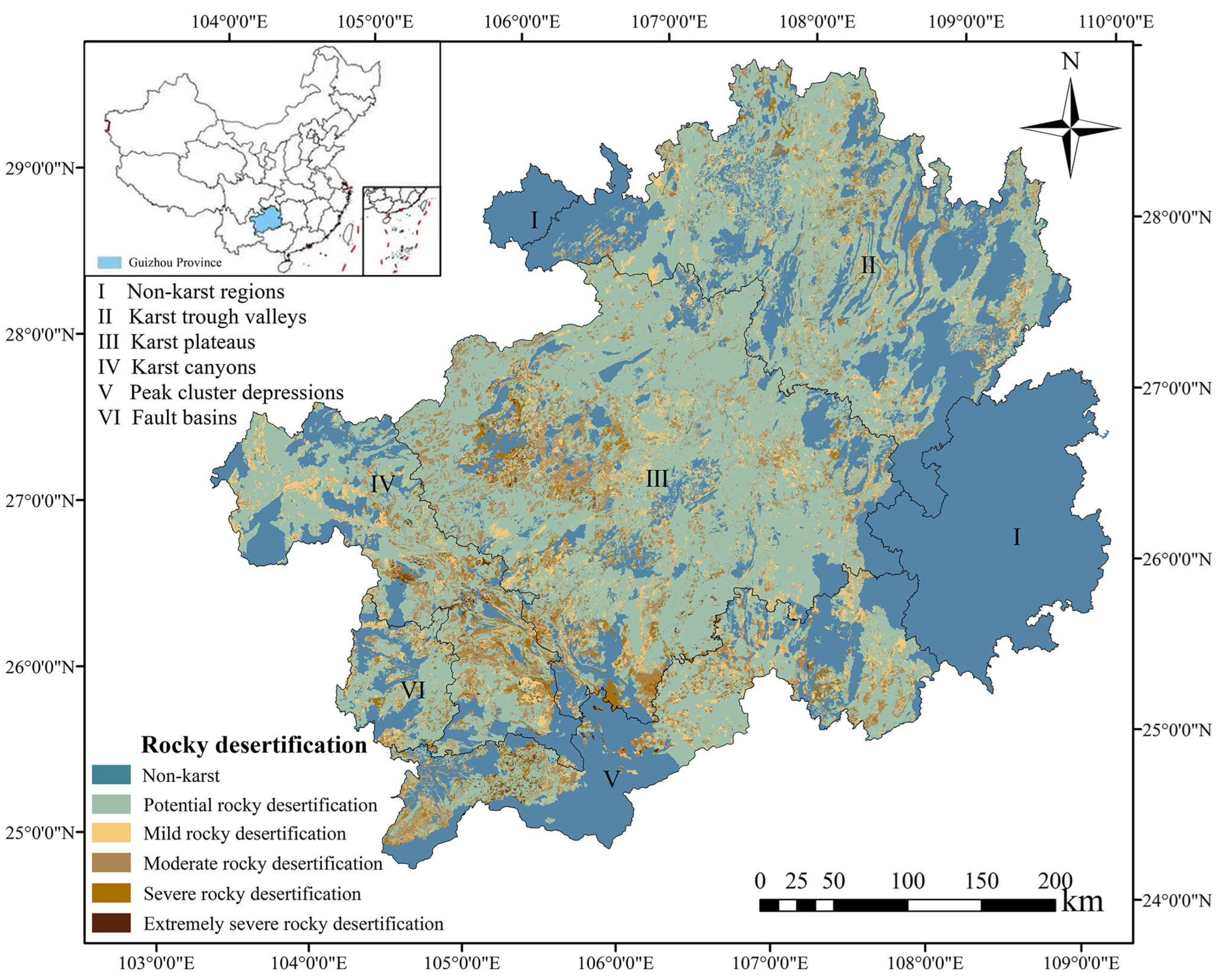
This study established a comprehensive zoning system based on the degree of karst development, landform type classification, and rocky desertification grades (Figure 1). The geographical distribution and geomorphic features of the six major regions are as follows: 1. Non-karst area: Mainly distributed in the Qiandongnan region. This area is dominated by clastic rock mountains and hills, with very few carbonate rocks. The soil layer is relatively thick (>50 cm), and vegetation coverage is high (forest coverage rate >60%). 2. Karst trough valley area: Mainly distributed in northern and central Guizhou. This area features long, strip-shaped valleys with peak clusters or peak forests on both sides. The valley bottom is flat, the soil layer is thin (20–50 cm), and the bedrock exposure rate is medium (10–30%). It is prone to mild rocky desertification. 3. Karst plateau area: Mainly distributed in the central, western, and southwestern parts of Guizhou Province. This area is a karst plateau surface at an altitude of 1000–1400 m, with widespread karst mounds and depressions. The surface is short of water, the soil layer is extremely thin (<20 cm), and the bedrock exposure rate exceeds 40%. 4. Peak cluster and depression area: Mainly distributed in southern and southwestern Guizhou. This area features a combination of dense conical peak clusters and closed depressions. Underground rivers are well-developed. The soil layer at the bottom of depressions is slightly thicker (30–60 cm), while bedrock exposure on the slopes of peak clusters exceeds 50%. 5. Fault depression basin area: Mainly distributed in western and southwestern Guizhou. The topographic feature of this area is a basin controlled by a fault zone, with steep edges and a flat bottom. The soil layer inside the basin is relatively thick (40–80 cm), and the potential risk of rocky desertification is high. 6. Karst canyon area: Mainly distributed in the middle and lower reaches of the Beipan River and the Wujiang River. The topographic features of this area include deep canyons, steep bank slopes (>45°), and a vertical height difference of >500 m. The soil layer is extremely thin (<10 cm), and the bedrock exposure rate exceeds 60%.

2.2. Research Technology Flow Chart

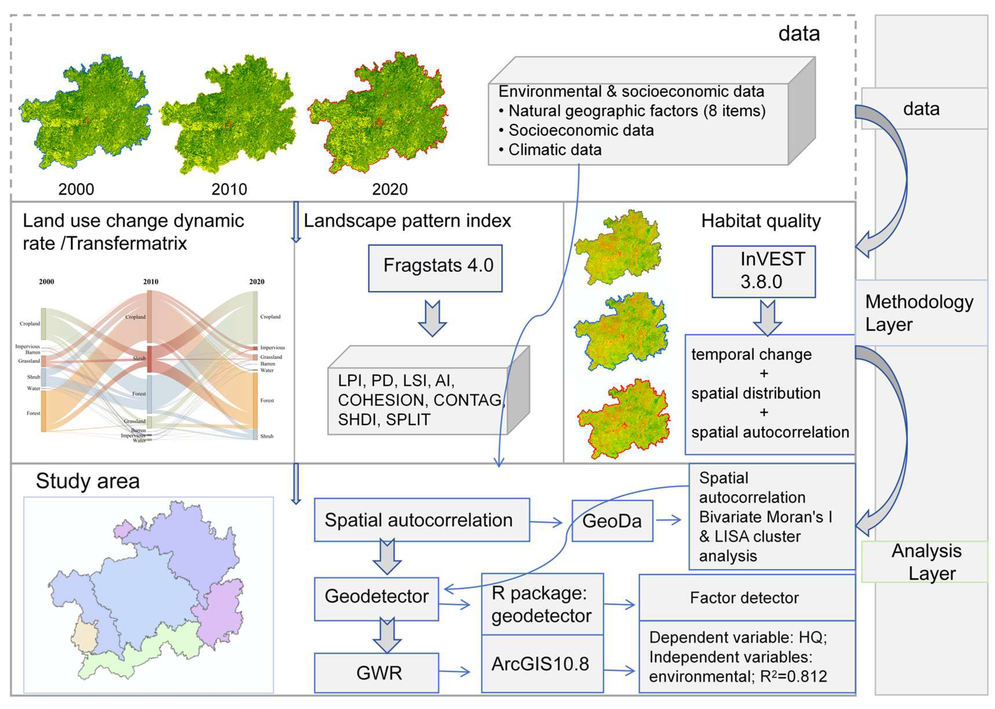
First, we used ArcGIS 10.8 to process land-use data for three periods (2000, 2010, and 2020). We then analyzed land-use transitions and calculated landscape pattern indices using Fragstats 4.0. Subsequently, we employed the InVEST 3.8.0 model to simulate the spatiotemporal distribution of habitat quality (HQ). Next, we conducted bivariate Moran’s I and LISA cluster analyses in GeoDa 1.20 to identify spatial autocorrelation. Finally, we used multi-source auxiliary data—including eight natural geographic factors, climatic variables, and socioeconomic indicators—as inputs to the Geodetector model (implemented via the R geodetector package, version 1.0-5, in R 4.0.0), quantifying each factor’s independent explanatory power. Additionally, we used the GWR module in ArcGIS 10.8 to reveal spatial heterogeneity in driving forces (Figure 2).

2.3. Data Sources and Processing

The land-use/land-cover (LULC) data used in this study were obtained from the Data Center for Resources and Environmental Sciences, Chinese Academy of Sciences [38], with a spatial resolution of 30 m. The administrative boundary of Guizhou Province was extracted using data from the Tianditu Cloud Platform [39]. GDP data were obtained from the China GDP Spatial Distribution Kilometer Grid Dataset (Resource and Environmental Science Data Center, Chinese Academy of Sciences) [40]; population density data were obtained from the 1990–2020 China Population Spatial Distribution Kilometer Grid Dataset (Institute of Geographic Sciences and Natural Resources Research, Chinese Academy of Sciences) [41].

Table 1. Data sources.

Type	Name	Units	Data Source
Basic Data	Guizhou Province Land-Use Data	/	Data Center for Resources and Environmental Sciences, Chinese Academy of Sciences [38]
	Administrative Boundaries of Guizhou Province	/	Administrative Division Data of China_Approval Number: GS(2024)0650 [39]
Natural Drivers	Digital Elevation Model (DEM)	m	Geospatial data cloud [42]
	Slope	°	Extraction based on DEM
	Soil Type	/	Resources and Environmental Science and Data Center, Chinese Academy of Sciences [43]
	Karst landform	/	Guizhou Rocky Desertification Control Center
	Soil layer thickness	/	Guizhou Rocky Desertification Control Center
	Comprehensive coverage of vegetation	/	Guizhou Rocky Desertification Control Center
	The exposure rate of bedrock	/	Guizhou Rocky Desertification Control Center
	Rocky desertification type	/	Guizhou Rocky Desertification Control Center
Socioeconomic Drivers	GDP	/	[40]
	Population Density	/	[41]

lists all the data used in this study and their sources. The natural geographic data include DEM, karst landform, soil type, slope, soil layer thickness, comprehensive vegetation coverage, bedrock exposure rate, and degree of rocky desertification. These data were sourced from the Geospatial Data Cloud, the Rocky Desertification Prevention and Control Center of Guizhou Province, and the Center for Resources and Environmental Sciences and Data of the Chinese Academy of Sciences. All data were then imported into ArcGIS 10.8, clipped to each county’s administrative boundary, and rasterized.

2.4. Research Methodology

2.4.1. Rate of Change in Land-Use Dynamics

The dynamic rate of land-use change quantitatively describes the magnitude and speed of area change for a specific LULC type over a given period. The formulas are as follows:

$$LC={\displaystyle \frac{U_b-U_a}{U_a}}\times {\displaystyle \frac{1}{T}}\times 100\%$$

(1)

$$LCG=\left({\displaystyle \frac{{\displaystyle {\sum }_{i=1}^n}{△LU}_{i-j}}{2{\displaystyle {\sum }_{i=1}^n}{LU}_i}}\right)\times {\displaystyle \frac{1}{T}}\times 100\%$$

(2)

where LC is the dynamic rate of a specific LULC type, U_a and U_b are the areas of that type at the initial and final stages, respectively; LCG is the integrated LULC dynamic rate; LU_i is the area of LULC type i at the initial stage; ΔLU_i-j is the absolute area converted from LULC type i to other types; and T is the study period in years [44].

2.4.2. Land-Use Transfer Matrix

The land-use transfer matrix reveals the dynamic transformation processes among LULC types, including transformation direction and structure. The matrix is defined as follows:

$$G_{xy}=\left[\begin{array}{cccc}{G}_{11}& G_{12}& \cdots & G_{1n}\\ G_{21}& G_{22}& \cdots & G_{2n}\\ \cdots & \cdots & \cdots & \cdots \\ G_{\mathrm{n}1}& G_{\mathrm{n}2}& \cdots & G_{\mathrm{n}n}\end{array}\right]$$

(3)

where n is the number of LULC types, x and y represent the LULC types at the initial and final stages, respectively, and G_xy is the area converted from type x to type y [45].

2.4.3. Landscape Pattern Index

A 1 km × 1 km grid was used as the analysis unit, following previous studies [46,47]. Given that Fragstats 4.0 can compute numerous landscape metrics, we performed a preliminary screening to reduce redundancy and information overlap. Candidate indices were subjected to Spearman’s rank correlation analysis, followed by principal component analysis (PCA) based on the approach [48]. Highly correlated indices were eliminated. The eight selected indices—Largest Patch Index (LPI), Patch Density (PD), Landscape Shape Index (LSI), Aggregation Index (AI), Cohesion Index (COHESION), Contagion Index (CONTAG), Shannon’s Diversity Index (SHDI), and Splitting Index (SPLIT) (

Table 2. Landscape pattern indices used in this study.

Category	Index	Description	Formula	Annotation
Landscape area index	Maximum Patch Index (LPI)	The higher the dominant degree of the largest patch in the landscape, the better the habitat quality	$\mathit{LPI}={\displaystyle \frac{\mathrm{MAX}(a_{\mathit{ij}})}{A_{total}}}\times 100\%$	aij = area of patchij (m2); A = Total landscape area (m2).
Landscape quantity index	Patch density (PD)	Number of patches per 100 hectares of landscape	$\mathit{PD}= \mathit{NP}/A$	NP = the total number of patches in the landscape; A = Total landscape area (m2).
Landscape shape index	Landscape Shape Index (LSI)	It mainly reflects the complexity of the patch shape in the landscape.	$\mathit{LSI}={\displaystyle \frac{0.25L}{\sqrt{A_{total}}}}$	A = Total landscape area (m2).
Landscape aggregation index	Aggregation index(AI)	The higher the degree of landscape fragmentation, the better the habitat quality	$AI={\displaystyle \frac{1}{2}}\left[1-{\displaystyle \frac{{\sum }_{i=1}^m{\sum }_{j=1}^m\frac{y_{ij}}{{\mathrm{m}\mathrm{a}\mathrm{x}}_{\left(g_{ij}\right)}}{\left(1-p_{ii}\right)}^2}{{\left(1-\frac{1}{m}\right)}^2}}\right]$	m = the total number of patch types in the landscape; gij = the total boundary length between patch type i and patch type j; max(gij) = the maximum possible boundary length between all pairs of patch types; pii = the proportion of the internal boundary of patch type i.
Landscape connectivity index	Cohesion index (COHESION)	The stronger the connectivity within the landscape, the worse the habitat quality.	$\mathit{COHESION}={\displaystyle \frac{1-\frac{{\sum }_{j=1}^m{p}_{ij}}{{\sum }_{j=1}^m{p}_{ij}\sqrt{a_{ij}}}}{1-\frac{1}{\sqrt{A}}}}\times 100$	aij = the area of patch j in Class i landscape; Pij is the perimeter (m) of patch j in a Class i landscape.
Landscape spread index	Spread index (CONTAG)	It can describe the agglomeration degree or extension trend of patch types in the landscape, including spatial information.	$\mathit{CONTAG} ={\displaystyle \sum _{i=1}^m}{\displaystyle \sum _{j=1}^m}{\displaystyle \frac{g_{\mathit{ij}}\times \left({\pi }_{\mathit{ij}}+{\pi }_{\mathit{ji}}\right)}{2\times m^2}}$	m = the total number of patch types in the landscape; gij = the adjacency probability between plaque type i and plaque type j; πij is the frequency adjacent to plaque type i and plaque type j; πji is the frequency adjacent to patch type j and patch type i.
Landscape diversity index	Shannon’s Diversity Index (SHDI)	Measures the diversity and heterogeneity of landscape patch types. Larger values indicate higher diversity and more even distribution.	$\mathit{SHDI} =-{\displaystyle \sum _{i=1}^m}\left(p_i\times \mathrm{l}\mathrm{n}{p}_i\right)$	pi = proportion of landscape occupied by patch type i.
Landscape fragmentation index	Fission index (SPLIT)	This metric evaluates both the spatial distribution pattern of the specified patch type and its isolation from other patch types in the landscape.	$\mathit{SPLIT} ={\displaystyle \frac{1}{2}}{\displaystyle \sum _{i=1}^m}{\displaystyle \frac{g_{\mathit{ij}}}{A_i}}$	m = the total number of patch types in the landscape; gij = the adjacency probability between plaque type i and plaque type j.

)—cover multiple dimensions of landscape characteristics, including area dominance, fragmentation, shape complexity, aggregation, connectivity, spread, diversity, and fragmentation. All landscape pattern index calculations were performed in Fragstats 4.0.

2.4.4. InVEST Model for Habitat Quality Assessment

The InVEST (Integrated Valuation of Ecosystem Services and Tradeoffs) Habitat Quality module evaluates habitat quality by integrating habitat type sensitivity and external threat intensity. All calculations were conducted using InVEST version 3.8.0.

Accurate parameter assignment is essential for reliable habitat quality assessment. In this study, threat factors were identified from LULC data, including cropland, urban land, rural residential land, other construction land, and unused land. The maximum stress distances, weights, and attenuation types for each threat factor (

Table 3. Threat factor weighting table.

Threat Factor	Maximum Influence Distance/km	Weight	Decaying Linear Dependence
Plowland	1	0.7	linearity
Urban construction land	8	1	exponent
Rural residential land	6	0.8	exponent
Other construction land	4	0.4	linearity
Unutilized	4	0.4	linearity

) were determined according to the InVEST model manual and previous studies in karst regions of Southwest China [25,49]. The habitat suitability and sensitivity scores for each habitat type with respect to each threat factor (

Table 4. Threat factor sensitivity table.

Land Class Types	Habitat Suitability	Plowland	Urban Construction Land	Rural Residential Land	Other Construction Land	Unutilized
Paddy field	0.4	0	0.7	0.6	0.6	0.5
Dry land	0.3	0	0.7	0.6	0.6	0.5
Forest land	1	0.7	0.8	0.3	0.3	0.6
shrubbery	0.8	0.8	0.6	0.4	0.4	0.6
Open forest land	0.7	0.7	0.7	0.5	0.5	0.6
Basal forest land	0.6	0.6	0.7	0.5	0.5	0.6
High cover grassland	0.8	0.8	0.5	0.7	0.7	0.5
Medium coverage grassland	0.7	0.7	0.7	0.5	0.5	0.3
Low cover grassland	0.6	0.5	0.7	0.5	0.5	0.4
River and canal	0.8	0.8	0.6	0.6	0.8	0.3
lakes	0.9	0.7	0.7	0.7	0.4	0.5
Reservoir pit	0.6	0.7	0.6	0.7	0.5	0.5
Bottom land	0.6	0.6	0.7	0.3	0.5	0.5
Urban land	0	0	0	0	0	0
Rural residential area	0	0	0	0	0	0
Other construction land	0	0	0	0	0	0
Special land	0	0	0	0	0	0
Marshland	0.6	0.5	0.5	0.5	0.5	0.1
Bare land	0.1	0.1	0.1	0.1	0.1	0.1
Bare rock stony land	0.1	0.1	0.1	0.1	0.1	0.1

) were defined using the same approach, with reference to local environmental conditions and expert knowledge. These parameter settings are consistent with established practices for habitat quality assessment in ecologically fragile karst areas.

The habitat degradation degree Dxj for raster in habitat type j is calculated as follows:

$$D_{xj}=\sum _{r=1}^R\sum _{y=1}^{Y_r}(w_r/\sum _{r=1}^R{w}_r)r_y{i}_{rxy}{\beta }_x{S}_{jr}$$

(4)

where R is the number of threat sources; w_r is the weight of threat source r; Y_r is the number of rasters of threat elements; r_y is the threat intensity of raster y; β_x is the accessibility level of threat sources to raster x (ranging from 0 to 1 based on legal protection); S_jr is the sensitivity of habitat type j to threat source r; and i_rxy is the stress effect of raster y on raster x, which follows either linear or exponential decay:

$$\mathrm{Linear} \mathrm{decay}:{ i}_{rxy}=1-{\displaystyle \frac{d_{xy}}{d_{r\mathrm{m}\mathrm{a}\mathrm{x}}}}$$

(5)

$$\mathrm{exponential} \mathrm{decay}: { i}_{rxy}=\mathrm{e}\mathrm{x}\mathrm{p}\left(-{\displaystyle \frac{{2.99d}_{xy}}{d_{r\mathrm{m}\mathrm{a}\mathrm{x}}}}\right)$$

(6)

where d_xy is the Euclidean distance between raster x and y, and d_rmax is the maximum influence distance of threat source r. Habitat quality Q_xj is then computed as follows:

$$Q_{xj}=H_j\left[1-\left({\displaystyle \frac{D_{xj}^z}{{D_{xj}^z+k}^z}}\right)\right]$$

(7)

where H_j is the habitat suitability of habitat type j (0 ≤ H_j ≤ 1); k is the half-saturation constant, generally set to 0.5; and z is a scaling constant, typically set to 2.5 [25,49,50,51]. The habitat type of interest was assigned a value of 1, and all other land classes were assigned 0. The LULC data for 2000, 2010, and 2020 were preprocessed through vectorization, reclassification, and raster calculation in ArcMap 10.8 before being input into the InVEST model. Subsequently, the calculated habitat quality values were categorized into five classes following previous studies [52]: I (0–0.2), II (0.2–0.4), III (0.4–0.6), IV (0.6–0.8), and V (0.8–1).

2.4.5. Bivariate Spatial Autocorrelation Analysis

Using ArcGIS 10.8, we resampled the study area into 1 km × 1 km grids and applied a bivariate spatial autocorrelation model to analyze the spatial correlation between landscape pattern indices and habitat quality. GeoDa 1.20 software was used for exploratory spatial data analysis, including autocorrelation statistics and outlier detection [9,53]. Local spatial autocorrelation was examined using local indicators of spatial association (LISA) to identify local clustering and dispersion effects [54,55].

The bivariate global Moran’s I is calculated as follows:

$$I_{sr}={\displaystyle \frac{n{\sum }_{i=1}^n{\sum }_{j=1}^n{w}_{ij}\left(\frac{y_{i.s}-{\overline{y}}_s}{{\sigma }_s}\right)\left(\frac{y_{i.r}-{\overline{y}}_r}{{\sigma }_r}\right)}{\left(\mathrm{n}-1\right){\sum }_{i=1}^n{\sum }_{j=1}^n{w}_{ij}}}$$

(8)

where I_sr is the bivariate global autocorrelation coefficient between habitat quality (s) and a landscape pattern index (r); y_i.s and y_i.r are the values of habitat quality and the landscape pattern index for unit i; $\overline{\mathrm{y}}$_s and $\overline{\mathrm{y}}$_r are their respective means; ${\mathsf{\sigma }}_{\mathrm{s}}$ and ${\mathsf{\sigma }}_{\mathrm{r}}$ are the standard deviations; w_ij is the spatial weight matrix based on adjacency; and n is the number of evaluation units. LISA cluster maps were generated to visualize spatial correlations, where high–high and low–low clusters indicate positive spatial correlation, and high–low and low–high clusters indicate negative spatial correlation.

2.4.6. GeoDetector-Based Attribution Analysis

We employed the factor detection module of the GeoDetector model to quantify the explanatory power of each driving factor for habitat quality spatial variation [56]. The q-statistic is defined as follows:

$$q=1-{\displaystyle \frac{{\sum }_{h=1}^L{N}_h{\sigma }_h^2}{\mathrm{N}{\sigma }^2}}$$

(9)

where h = 1, …, L are the strata of factor X; N_h and N are the number of sampling units within stratum h and across the whole area, respectively; σ²_h and σ² are the variances of Y within stratum h and across the whole area. The q-value ranges from 0 to 1 and represents the proportion of the spatial variance of Y explained by factor X [57].

All spatial analyses were conducted on a regular 1 km × 1 km grid, as used in the landscape pattern and spatial autocorrelation analyses. Driving factors were grouped into three categories: (1) purely natural factors (DEM, slope, soil type, soil thickness, karst landform, bedrock exposure rate); (2) compound factors (vegetation coverage, degree of rocky desertification); (3) purely anthropogenic factors (type of land-use change, land-use intensity, GDP, population density). To account for the shifting dominance of drivers, we assigned period-specific weights to compound factors: 80% natural and 20% anthropogenic for 2000–2010, and 30% natural and 70% anthropogenic for 2010–2020. This adjustment reflects the documented transition in the Guizhou karst region [58,59,60,61], where natural constraints dominated in the 2000s, while anthropogenic pressures intensified markedly after 2010.

2.4.7. Geographically Weighted Regression (GWR) Model

Given that global linear regression models may fail to reveal locally varying relationships between natural geographic factors and habitat quality due to spatial non-stationarity, we adopt geographically weighted regression (GWR) to capture such local heterogeneity. Geographically weighted regression (GWR) is a spatial analysis technique that captures spatial non-stationarity by constructing local regression equations at different locations [62,63]. The GWR model is expressed as follows:

$$y_i={\beta }_0\left(u_i,v_i\right)+{\displaystyle \sum _{k=1}^p}{\beta }_k\left(u_i,v_i\right)x_{ik}+{\epsilon }_i$$

(10)

where (u_i, v_i) are the coordinates of sampling point i; $\beta$_k(u_i, v_i) is the local regression coefficient for the k-th explanatory variable at point i; X_ik is the value of the k-th explanatory variable at point i; and ${\epsilon }_{\mathrm{i}}$ is the random error term. The adaptive bandwidth was determined using the corrected Akaike Information Criterion (AICc), and the weighting function used was the adaptive bi-square kernel.

Prior to GWR implementation, multicollinearity diagnostics were performed for all explanatory variables. The variance inflation factor (VIF) for each variable was examined using ordinary least squares (OLS) regression; all VIF values were below 10 [64], indicating no severe global multicollinearity. Local collinearity diagnostics were also conducted using the GWmodel package (version 2.4-1) in R 4.0.0 [65], and no significant local collinearity issues were detected. The eight natural geographic factors (DEM, karst landform, soil type, slope, soil layer thickness, comprehensive vegetation coverage, bedrock exposure rate, and rocky desertification type) were used as explanatory variables, with habitat quality (HQ) as the dependent variable. Spatial variability maps of the regression coefficients were generated to visualize the spatially heterogeneous effects of these factors on HQ.

To establish a clear hierarchy of the driving factors, we developed a Composite Importance Index (CII) from three metrics derived from the GWR local coefficient estimates: (1) the mean of the absolute local regression coefficients, indicating influence intensity; (2) the proportion of sampling sites with statistically significant local coefficients (|t| > 1.96), indicating reliability; (3) the standard deviation of the absolute coefficients, indicating spatial heterogeneity. For each metric, we ranked the variables separately from highest to lowest, then calculated the CII as a weighted sum of the three ranks: CII = 0.4 × Rank_Intensity + 0.35 × Rank_Reliability + 0.25 × Rank_Heterogeneity. We assigned the largest weight to influence intensity (40%), followed by reliability (35%) and heterogeneity (25%), following common practice in composite indicator construction [66]. This weighting reflects our primary aim of identifying factors with strong and consistent effects, as well as spatially varying influences. Based on the CII scores, we classified the driving factors into four tiers of importance (Tiers I–IV), with lower CII values indicating greater overall importance. This tiered classification provides a transparent, reproducible basis for prioritizing management interventions across different karst zones.

3. Results

3.1. Spatial and Temporal Changes in Land Use

3.1.1. Temporal Changes in Land Use

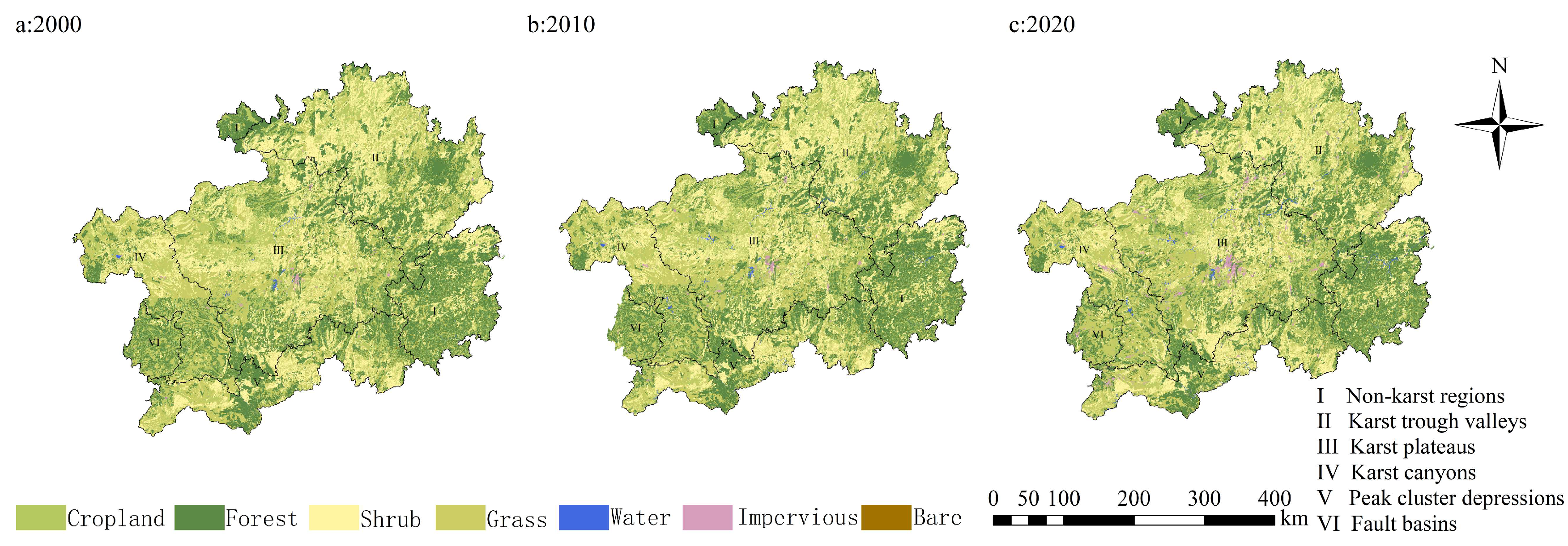
Overall, from 2000 to 2020, cropland and forested land increased modestly, and construction land expanded. Meanwhile, shrubland and grassland declined (

Table 5. The dynamic rate of change of different LULC classes in the study area from 2000 to 2020.

LULC Type	2000–2010	2010–2020	2000–2020
Cropland	1.87%	−1.43%	0.44%
Forest	−0.96%	2.68%	1.72%
Shrub	−0.54%	−1.36%	−1.90%
Grassland	−0.61%	−0.35%	−0.96%
Water	0.08%	0.06%	0.15%
Barren	0.00%	0.00%	0.00%
Impervious	0.16%	0.39%	0.55%

). Table 5 shows that cropland and forested land increased at annual rates of 0.44% and 1.72%, respectively, and remained the dominant types. Meanwhile, construction land expanded at a dynamic rate of 0.39% during 2010–2020. For ecological land use, the total area decreased, mainly due to rapid declines in shrubland (–1.90%) and grassland (–0.96%). In contrast, the water area showed a general increasing trend, with a relatively stable rate of change of 0.15%. The combined land-use dynamics for the periods 2000–2010 and 2010–2020 were 6.78% and 7.21%, respectively, indicating an increase in the intensity of human activities. All land-use types changed during the study period, and land-use changes were more rapid between 2010 and 2020. The spatial distribution of land-use types from 2000 to 2020 is shown in Figure 3.

3.1.2. Spatial Changes in Land Use

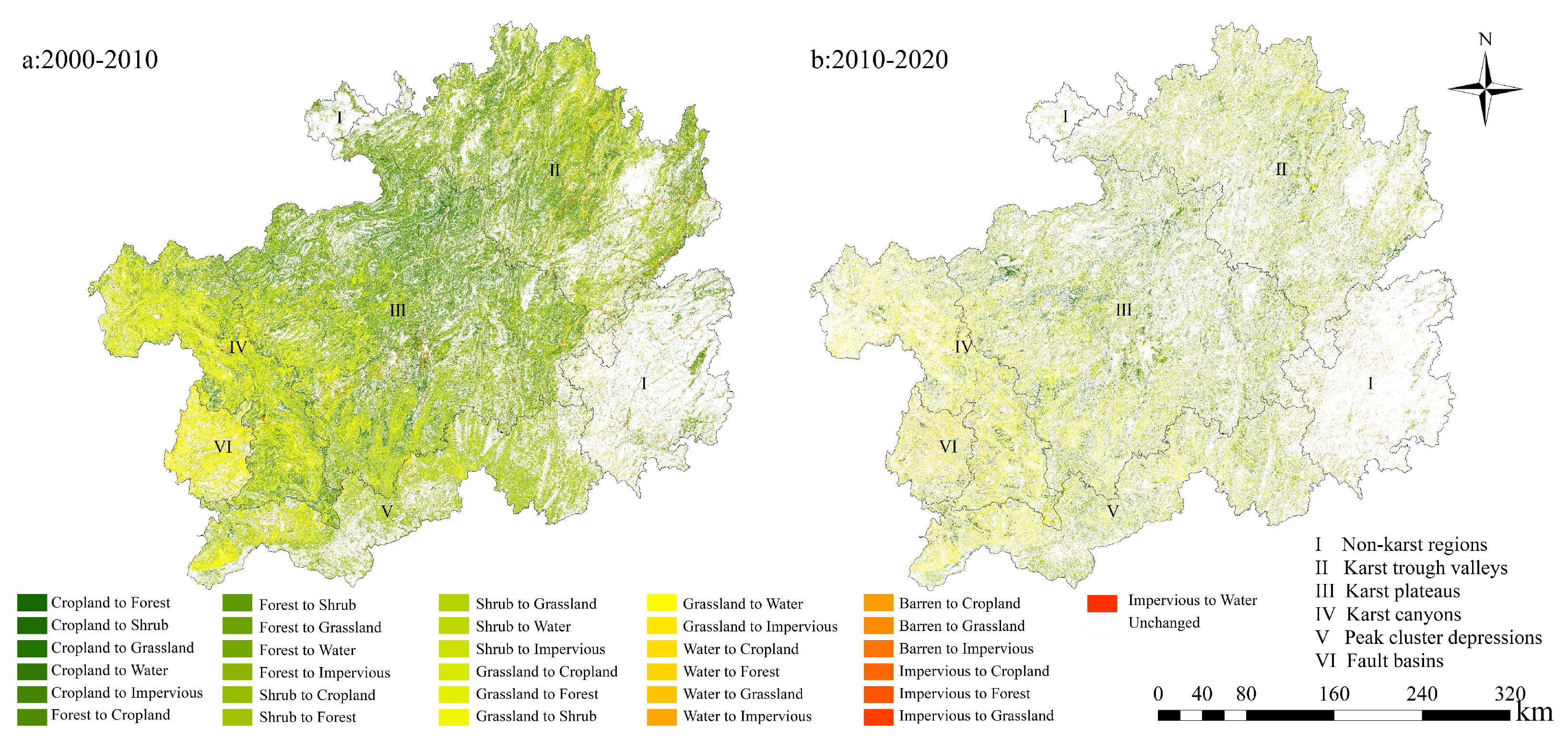
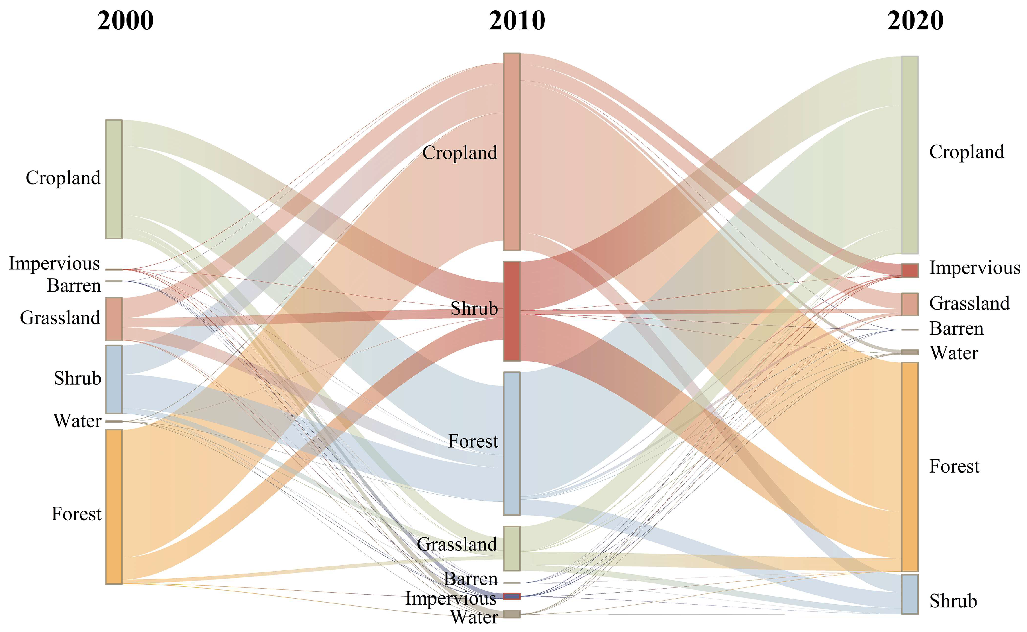
Overall, the spatial pattern of land-use change shifted from karst canyons, peak-cluster depressions, and faulted basins in 2000–2010 to karst plateaus and trough valleys in 2010–2020, with a notable increase in cropland conversion. Between 2000 and 2010, most land-use changes occurred in areas such as karst canyons, peak-cluster depressions, and faulted basins, and were mainly conversions among farmland, forests, and shrublands. The hotspot areas for conversions shifted to karst plateaus and trough valleys during 2010–2020, and the types of land-use changes increased, with arable land converted out accounting for 43.01% of the total converted area.

During 2000–2010, forest land accounted for the largest proportion of converted area, at 40.03%. During 2010–2020, cropland became the main type of conversion, with a conversion share of 43.01% (Figure 4 and Figure 5). Specifically, between 2000 and 2020, 308.97 km² of cropland was converted to construction land, accounting for 5.47% of the total area transferred out of cropland. During this period, the transfer of ecological land (including grasslands, forests, and water bodies), with converted areas of 25.56 km², 21.49 km², and 4.90 km^2, respectively, also contributed to the sustained increase in construction land area. However, only 2.13 km² of non-ecological land was converted into ecological land, and this conversion was relatively dispersed, indicating weak ecological restoration effects. The conversion of 308.97 km² of arable land into construction land directly exacerbated habitat fragmentation.

3.2. Landscape Pattern Change Characteristics

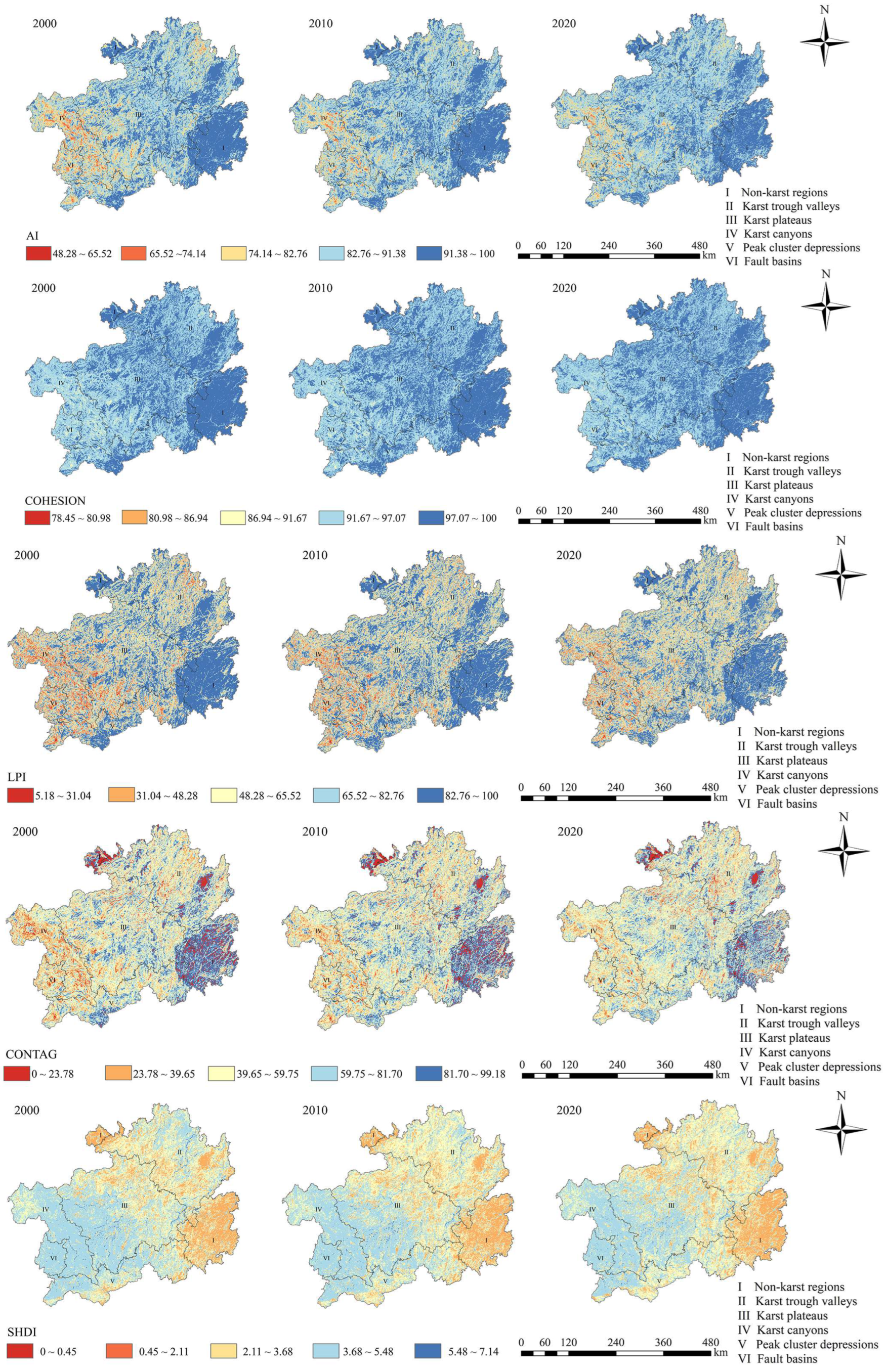
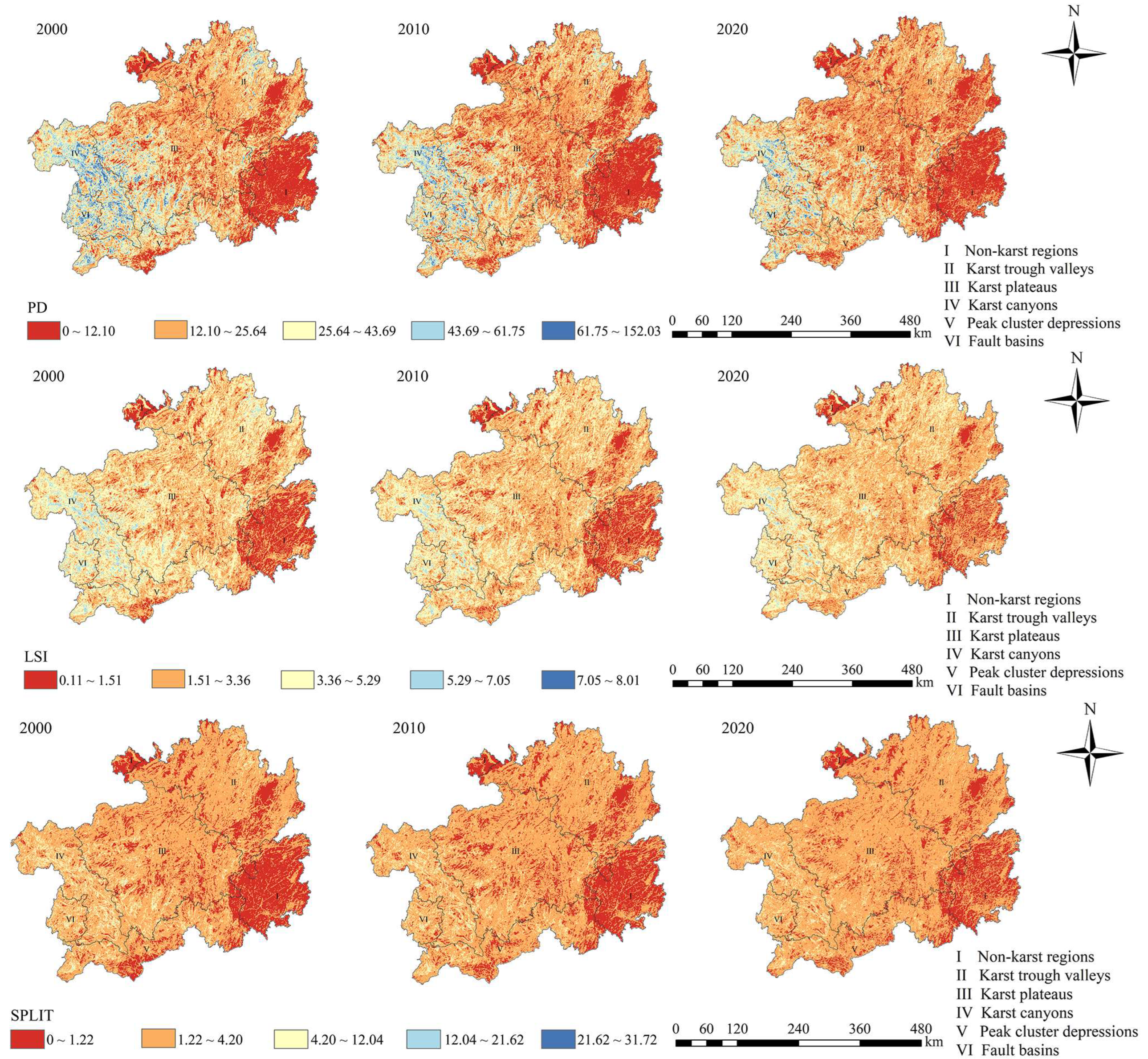
The spatio-temporal features of landscape pattern indices (LSPI), including AI, COHESION, LPI, CONTAG, SHDI, PD, LSI, and SPLIT, were selected for analysis, and ArcGIS was used to generate the spatio-temporal distribution maps of these indices, as shown in Figure 6.

AI (Aggregation Index) measures the degree of within-class patch aggregation or landscape continuity. A low AI value indicates small, dispersed, whereas a high AI value suggests they are physically clustered. The mean AI value increased from 88.3015 in 2000 to 88.7391 in 2020, indicating that land-use activities have led to continuous landscape aggregation. Higher AI values were mainly concentrated in non-karst areas, while lower AI values were mainly concentrated in karst canyons and faulted basin areas.

COHESION reflects the aggregated or dispersed state of patches and quantifies the physical connectivity of habitats for organisms dispersing across a binary landscape. During the study period, the mean COHESION values were 96.6891 in 2000, 96.8361 in 2010, and 96.7856 in 2020, showing a slightly increasing trend with little fluctuation. The spatial distribution was similar to that of AI, indicating the influence of human activities on landscape pattern. Non-karst areas had better vegetation cover and higher biodiversity.

LPI (Largest Patch Index) indicates the dominance of a particular landscape type. Higher LPI values suggest one or several very dominant patches, while lower values indicate a more homogeneous landscape with no particularly dominant patch. The LPI increased from 58.3044 in 2000 to 66.9573 in 2020, indicating a continued increase in landscape dominance. The spatial pattern of LPI resembled that of AI and COHESION. Low-value areas decreased significantly, and landscape types became more evenly distributed.

CONTAG (Contagion Index) measures the degree of cross-class adjacency and intermixing among different patch types. A higher CONTAG indicates good connectivity among some dominant patches. CONTAG decreased from 56.5393 in 2000 to 55.9076 in 2020, indicating that landscape connectivity (as reflected by cross-type adjacency) continued to weaken. The low-value zones of CONTAG decreased obviously, but remained locally concentrated in mountainous areas such as non-karst areas and karst trough areas. Higher-value zones were mostly distributed in the main urban cores of karst plateau zones, where the aggregation or expansion of different landscapes was significantly stronger.

SHDI (Shannon’s Diversity Index) describes the spatial distribution and diversity of different patch types. An SHDI value of zero indicates no diversity; larger values indicate higher diversity and more even distribution of patch types. Between 2000 and 2020, the SHDI value decreased slightly from 3.5272 to 3.5125, indicating a decrease in land-use diversification. This decline suggests that land use became more intensive and the land-use structure became more stable, as fewer patch types dominated the landscape. At the spatial scale, high SHDI values were found in areas with frequent human activities, such as karst plateaus, karst canyons, and faulted basins. Low SHDI values were mainly concentrated in mountainous areas or basins.

PD (Patch Density) describes the degree of landscape fragmentation. A higher PD value indicates a higher degree of fragmentation, while a lower PD value indicates a more continuous landscape with less fragmentation. Between 2000 and 2020, PD decreased from 22.8563 to 20.2019, indicating that land-use fragmentation was reduced. At the spatial scale, high PD values were in areas with frequent human activities, such as karst plateaus, karst canyons, and faulted basins, where urban agglomerations or continuous concentrated croplands are more developed, anthropogenic impacts are more pronounced, and landscapes tend to be more fragmented. Low PD values were mainly concentrated in non-karst areas.

LSI (Landscape Shape Index) reflects the irregularity of patch boundaries and the complexity of patch shapes. Larger LSI values indicate more complex, zigzagging boundaries and irregular shapes. Smaller LSI values indicate simpler, more regular patch boundaries. LSI decreased from 3.0606 in 2000 to 2.9968 in 2020, suggesting that landscape patch shapes tended to become more regular. Conversely, urban and agricultural expansion caused by human activities can lead to increased LSI values and fragmentation of ecological processes, such as reduced biodiversity, declining ecological connectivity, and degradation of ecological functions. Higher LSI values were concentrated in karst plateaus, karst valleys, and fault basins.

SPLIT (Splitting Index) is generally lower in natural landscapes with less human disturbance and higher in areas with more human activity. SPLIT decreased from 2.3329 in 2000 to 2.2362 in 2010, then increased to 2.3024 in 2020, indicating that the condition of natural landscapes had stabilized to some extent. The spatial distribution pattern of SPLIT was similar to that of LSI, with lower core areas mainly concentrated in non-karst areas with better ecological environments, and higher values mainly concentrated in areas such as karst plateaus, karst canyons, and fault basins, attributed to high levels of human activity causing significant disturbance to the natural landscape.

The overall landscape pattern changes were as follows: patch aggregation increased (AI: 88.30→88.74; COHESION: 96.69→96.79), but landscape connectivity weakened, as indicated by CONTAG (CONTAG: 56.54→55.91); dominant patches became more centralized (LPI: 58.30→66.96); landscape diversity decreased and land use tended to intensify (SHDI: 3.53→3.51; PD: 22.86→20.20); patch shape regularity improved and fragmentation eased (LSI: 3.06→3.00; SPLIT: 2.33→2.30) after an initial decline and a subsequent increase.

3.3. Characterization of Changes in Habitat Quality

3.3.1. Spatial and Temporal Changes in Habitat Quality Classes

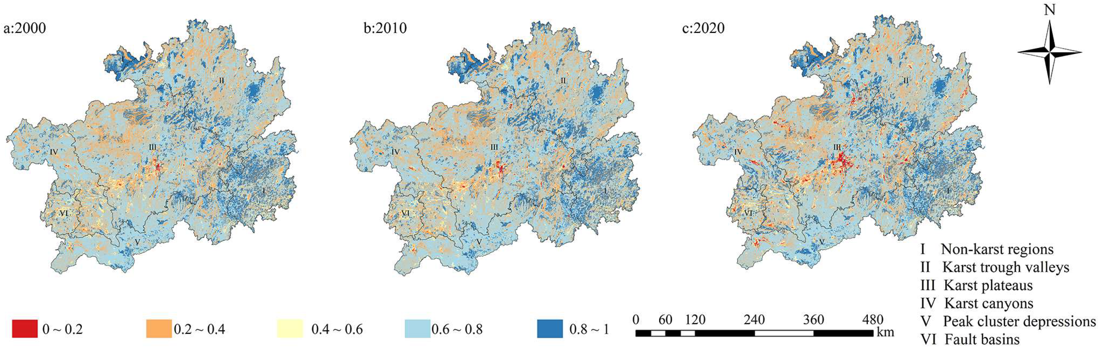
Overall, habitat quality in the study area declined between 2000 and 2020, with Class IV remaining dominant but decreasing in area. Notably, both the lowest-quality (Class I) and highest-quality (Class V) areas increased, but the expansion of Class I outpaced that of Class V. As a result, the average habitat quality dropped from 0.634 in 2000 to 0.606 in 2020, a decrease of 4.4%. Using ArcGIS 10.8 software, the habitat quality values were categorized into five classes based on previous studies [52]: I (0–0.2), II (0.2–0.4), III (0.4–0.6), IV (0.6–0.8), and V (0.8–1). The area of each class and its percentage of the total habitat area were calculated for the three time points (see

Table 6. Changes in Area and Percentage of Habitat Quality Classes in the study area from 2000 to 2020.

Habitat Quality Level	2000		2010		2020
	Area	Percentage	Area	Percentage	Area	Percentage
	km2	%	km2	%	km2	%
I	639.65	0.36%	904.07	0.51%	2445.09	1.39%
II	49624.28	28.18%	49401.70	28.05%	48268.09	27.41%
III	5251.61	2.98%	5285.86	3.00%	6030.39	3.42%
IV	96911.99	55.03%	95863.48	54.44%	92667.65	52.62%
V	23674.00	13.44%	24648.07	14.00%	26680.11	15.15%

). Specifically, habitat quality was dominated by Class IV, although its area decreased continuously from 96,911.99 km² to 92,667.65 km², and its percentage dropped from 55.03% to 52.62%. The second largest was Class II, which showed a small decrease in area from 49,624.28 km² to 48,268.09 km². All other classes increased in size between 2000 and 2020, with the most significant increases observed in Class I (from 0.36% to 1.39%) and Class V (from 13.44% to 15.15%).

Class V was mainly distributed in non-karst areas, which have less ground undulation, a variety of landform types (including hills, low mountains, and mid-mountains), a more developed surface water system, diverse soil types, better vegetation cover, and high biodiversity, thus supporting better habitat quality. Low habitat quality areas were concentrated in the karst plateau area. Lower habitat quality areas were concentrated in karst trough valleys, peak cluster depressions, and other areas with thin soil layers and even lower vegetation cover. In karst canyons and faulted basins, land-use types were mainly cropland and construction land, all of which have low biodiversity. Thus, the spatial distribution of habitat quality is closely related to natural geographic features, land-use types, and human activities. The spatial variation in classified habitat quality over the years is shown in Figure 7.

3.3.2. Degree of Habitat Degradation

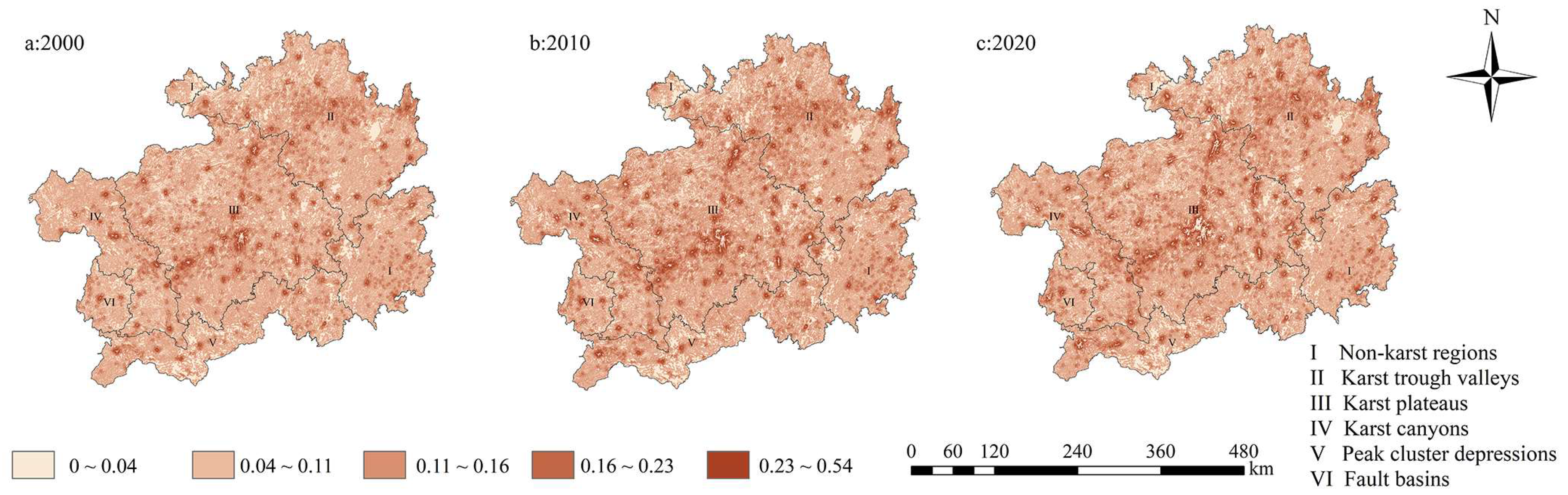
Habitat degradation, which refers to the extent to which a habitat is disturbed by threatening factors, is a key indicator of ecosystem disturbance. In this study, the degree of habitat degradation was calculated using the InVEST model for three time points (2000, 2010, and 2020), and its spatial distribution was mapped (Figure 8). Overall, habitat degradation in the study area remained low but increased over time, with a clear spatial expansion from the karst plateau to karst trough areas. The mean degradation value rose from 0.1002 in 2000 to 0.1081 in 2020. In 2000, areas with higher degradation were mainly concentrated in and around urban and construction land in the karst plateau region. By 2020, however, areas with higher degradation had expanded into karst trough areas. Specifically, over-cultivation, urban expansion, and irrational land use may lead to soil erosion, vegetation loss, wildlife habitat destruction, and biodiversity decline. This indicates that urbanization has had a serious negative impact on habitats.

3.4. Analysis of Landscape Pattern Effects on Habitat Quality

3.4.1. Spatial Autocorrelation Analysis

The LSPI and HQ data for 2000, 2010, and 2020 were imported into GeoDa 1.20 software, and correlation analyses were conducted between habitat quality and each LSPI. AI, COHESION, CONTAG, and LPI were positively correlated with habitat quality, while the other indices were negatively correlated. All correlation analyses were statistically significant (p < 0.01). Although these coefficients are derived from separate cross-sectional analyses for each year and do not represent a formal temporal trend (e.g., time series autocorrelation), their values increased consistently from 2000 to 2020 for all indices except CONTAG and SHDI, suggesting a strengthening of spatial association over the study period. The detailed global Moran’s I values are presented in

Table 7. Global Moran’s I values for landscape pattern index and habitat quality in the study area from 2000 to 2020.

Year	Value Type	AI and HQ	Cohesion and HQ	Contag and HQ	LPI and HQ	LSI and HQ	PD and HQ	SHDI and HQ	Split and HQ
2000	Moran′s I	0.451	0.336	0.394	0.415	−0.451	−0.435	−0.515	−0.280
	Z value	31.994	34.075	32.050	30.245	−31.930	−31.650	−37.258	−21.724
2010	Moran′s I	0.471	0.371	0.375	0.465	−0.476	−0.473	−0.476	−0.276
	Z value	32.019	32.098	32.935	31.492	−32.361	−32.500	−32.418	−22.361
2020	Moran′s I	0.485	0.385	0.385	0.476	−0.490	−0.488	−0.490	−0.290
	Z value	32.426	32.533	32.348	31.609	−32.881	−32.880	−32.915	−22.901

.

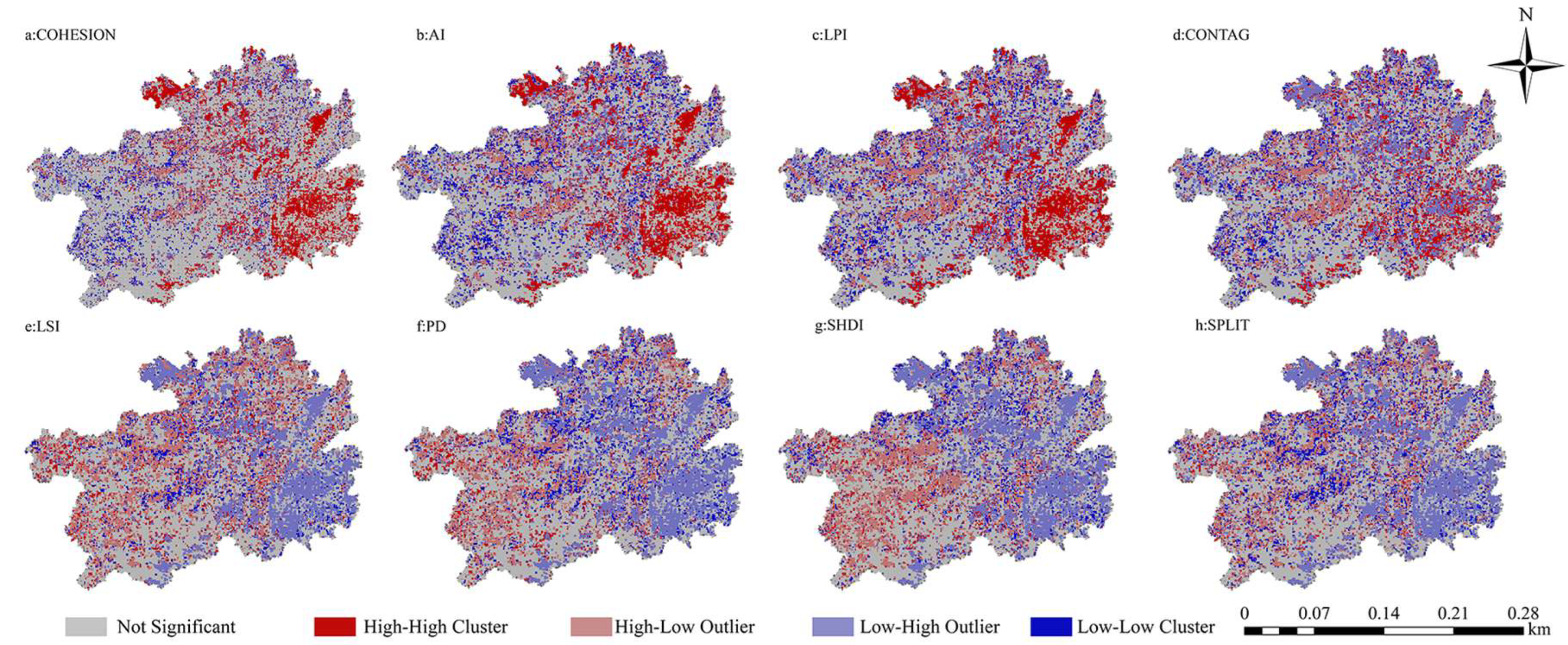
The results of the local spatial autocorrelation analysis are shown in

Table 8. Statistics of the number and percentage of agglomeration-type patches in 2020.

		Not Significant	High–High	Low–Low	Low–High	High–Low
AI	Quantity block	86629	33517	17435	10637	9916
	Percentage	54.78%	21.20%	11.03%	6.73%	6.27%
COHESION	Quantity block	86627	34318	16243	10236	10710
	Percentage	54.78%	21.70%	10.27%	6.47%	6.77%
CONTAG	Quantity block	86629	20747	27068	12407	11283
	Percentage	54.78%	13.12%	17.12%	7.85%	7.14%
LPI	Quantity block	88629	37041	15925	8513	8026
	Percentage	56.05%	23.42%	10.07%	5.38%	5.08%
LSI	Quantity block	86622	8698	35783	13457	13574
	Percentage	54.78%	5.50%	22.63%	8.51%	8.58%
PD	Quantity block	86624	7480	37432	14674	11924
	Percentage	54.78%	4.73%	23.67%	9.28%	7.54%
SHDI	Quantity block	86625	8274	36164	13880	13191
	Percentage	54.78%	5.23%	22.87%	8.78%	8.34%
SPLIT	Quantity block	86624	7264	38111	14891	11244
	Percentage	54.78%	4.59%	24.10%	9.42%	7.11%

. Cells with insignificant correlation for each indicator accounted for more than half of the total number of cells in the study area, indicating no spatial autocorrelation for those cells. CONTAG had a more balanced distribution of clusters, with the number of positively spatially correlated cells being closest to the number of negatively correlated cells. For the remaining indices, high–high and low–low clustering were generally more frequent than high–low and low–high clustering, and the number of positively correlated cells exceeded the number of negatively correlated cells. AI, COHESION, and LPI had significantly more high–high clusters than low–low, high–low, and low–high clusters, while LSI, PD, SHDI, and SPLIT had significantly more low–low clusters than high–high clusters.

The LISA clustering map showed five types of local spatial autocorrelation: “high-high,” “low-low,” “high-low,” “low-high,” and “not significant” (Figure 9). The “high-high” type indicates a clustering effect of high values of both landscape pattern indices and habitat quality. The “high-low” pattern indicates a clustering effect of high LSPI values and low HQ values. Differences in natural geographic features and hydrothermal conditions across different units of Guizhou Province led to varying responses of different LSPIs to HQ. The “high-high” and “low-low” clustering distributions of AI, COHESION, CONTAG, and LPI on HQ were more obvious at the 1 km × 1 km grid scale, indicating a positive correlation between these LSPIs and HQ, while the remaining indices showed a negative correlation with HQ. The spatial clustering characteristics of the eight LSPIs with respect to HQ differed from one another, reflecting spatial heterogeneity.

Due to spatial correlation, the relationship between LSPI and HQ followed certain patterns across regions. Analyzed according to different karst development areas in Guizhou Province, “high-high” clustering dominated in non-karst areas and karst troughs and valleys, while “low-low” clustering dominated in karst canyons and faulted basins. In the karst plateau area, the distribution of “low-high” and “high-low” clusters was intertwined, reflecting the complex coupling of anthropogenic disturbances and natural geographic conditions.

3.4.2. Driving Factor Attribution Analysis

To examine the influence of various factors on habitat quality in Guizhou, we applied the factor detection module of the GeoDetector model. The q-statistic measures each factor’s explanatory power for the spatial differentiation of habitat quality; all factors were significant (p < 0.05) in both periods. In 2000–2010, the leading factors were Slope (0.3214), VegCover (Vegetation Cover, 0.2785), RockyDes (Rocky Desertification, 0.2236), SoilThick (Soil Thickness, 0.2128), and LUCT (Land-Use/Cover Type, 0.1972). Natural and compound factors dominated, while pure anthropogenic factors had relatively low q-values. In 2010–2020, the ranking shifted to LUCT (Land-Use/Cover Type, 0.3168), VegCover (Vegetation Cover, 0.3142), LUI (Land-Use Intensity, 0.2274), GDP (Gross Domestic Product, 0.2149), and Slope (0.2036). Anthropogenic factors rose markedly—LUCT increased by 60.6% while GDP nearly doubled—whereas natural factors declined across the board. VegCover remained high, while RockyDes dropped noticeably.

This shift is equally evident at the aggregate level (

Table 9. Grouped q-value sums and attribution percentages by factor category.

Category	2000–2010 q-sum	2010–2020 q-sum	Contribution Shift
Pure natural	0.9423	0.7223	↓ 23.4%
Compound	0.5021	0.4795	↓ 4.5%
Pure anthropogenic	0.5516	0.9455	↑ 71.4%
Total	1.996	2.1473
Natural contribution	67%	40%	↓
Anthropogenic contribution	33%	60%	↑

Note: Contributions are presented as rounded percentages and should be interpreted as indicative trends rather than precise estimates. Arrows in the Contribution Shift column: ↓ = decrease from 2000–2010 to 2010–2020; ↑ = increase.

). In 2000–2010, the q-sum of pure natural factors (0.9423) far exceeded that of pure anthropogenic factors (0.5516), with a weighted natural contribution of approximately 67% and an anthropogenic contribution of approximately 33%. By 2010–2020, the q-sum of pure anthropogenic factors rose to 0.9455, while pure natural factors fell to 0.7223; the weighted anthropogenic contribution increased to approximately 60%, surpassing the natural contribution (approximately 40%). A sensitivity test varying the splitting weights by ±10% confirmed that the reversal in dominance—from natural in 2000–2010 to anthropogenic in 2010–2020—remained robust across all scenarios, with absolute contributions varying by ±3–5 percentage points.

Overall, the dominant drivers transitioned from natural landform and vegetation conditions in the early period to land-use change and economic development in the later period, indicating a clear shift from natural to anthropogenic dominance over the two decades.

3.4.3. Spatial Non-Equilibrium Analysis

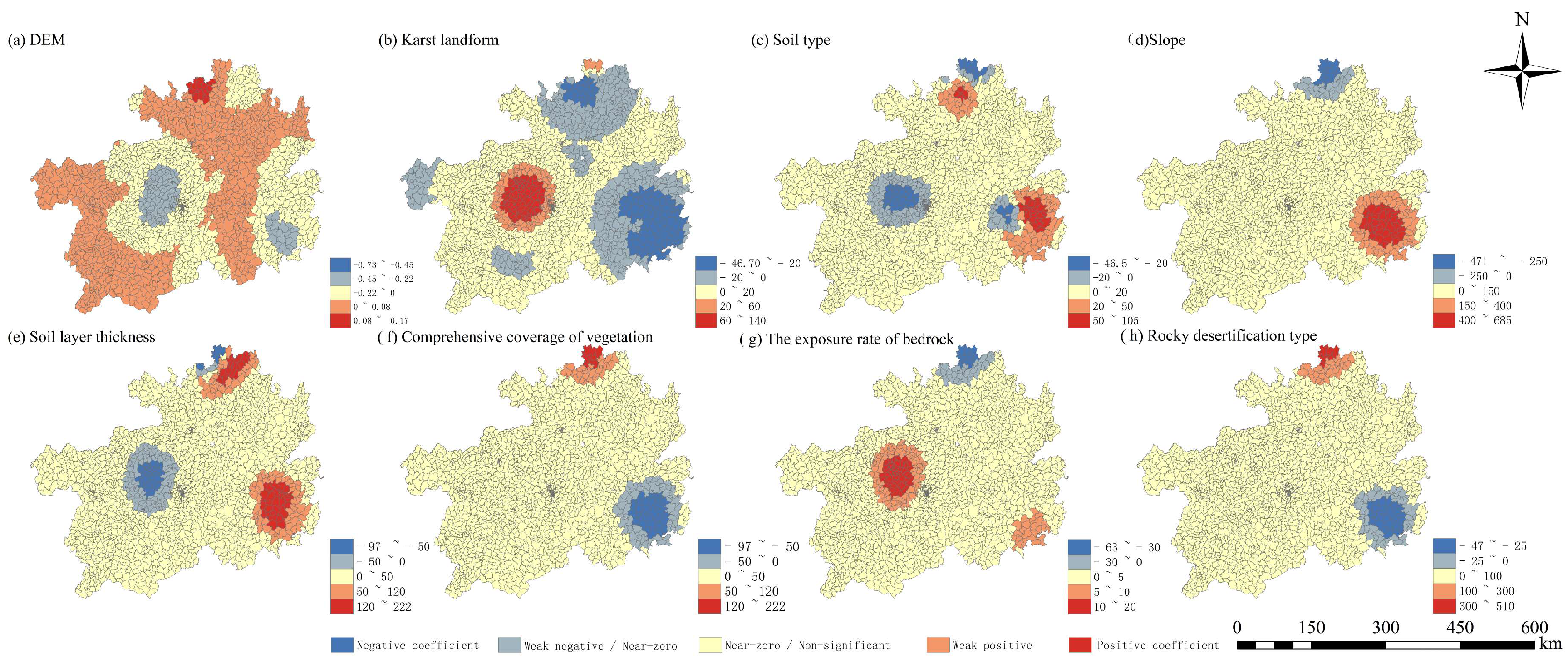
The GWR model was applied to capture spatially varying relationships between natural factors and habitat quality at the township level in 2020. The global OLS regression yielded an R² of only 0.417, whereas the GWR model achieved an R² of 0.812, confirming strong spatial non-stationarity and indicating that global regression fails to capture local variations in these relationships. Among the eight explanatory variables, slope exhibited the greatest spatial variation in coefficients ($\mathrm{S}\mathrm{D}=0.2278$), followed by bedrock exposure rate ($\mathrm{S}\mathrm{D}=0.2023)$, karst landform ($\mathrm{S}\mathrm{D}=0.1711)$, soil type ($\mathrm{S}\mathrm{D}=0.1298)$, and rocky desertification ($\mathrm{S}\mathrm{D}=0.1030)$. This ranking suggests that topographic and surface geological conditions—particularly slope, bedrock exposure, and karst landform—are the most context-dependent drivers of habitat quality in Guizhou’s karst landscape (

Table 10. This iSpatial variability ranking of local coefficients for natural factors.

Variable	Mean	Std. Dev.	CV	Rank
Bedrock exposure rate	0.0747	0.2023	2.71	1 (strongest)
Karst landform	−0.0526	0.1711	3.25	2
Slope	0.4429	0.2278	0.51	3
DEM	0.3019	0.3018	1	4
Vegetation cover	0.2102	0.1376	0.65	5
Rocky desertification	−0.0256	0.103	4.02 *	(CV inflated)
Soil thickness	−0.0248	0.1581	6.38 *	(CV inflated)
Soil type	−0.0041	0.1298	31.9 *	(CV inflated)

Note: * CV inflated due to near-zero mean; bedrock exposure rate is the ecologically meaningful primary source.

).

Slope had positive effects across all six karst zones (coefficients: 0.275–0.543), with more than 70% of local coefficients being significant in the karst canyon (0.692), karst plateau (0.772), and peak-cluster depression (0.711). However, this positive effect weakened considerably in steep-slope areas (>25°) within the karst plateau ($\mathrm{m}\mathrm{e}\mathrm{a}\mathrm{n}=0.28)$, compared to gently sloping basins ($\mathrm{m}\mathrm{e}\mathrm{a}\mathrm{n}=0.48$). In contrast to the zone-consistent behavior of slope, the remaining factors showed clear divergent patterns across zones (

Table 11. Sign, magnitude, and significance of GWR coefficients by zone.

Zone	Bedrock Exposure	Karst Landform	Slope	Soil Thickness	Rocky Desertification
Karst canyon	+ low ★	+ low ○	+ high ★	− medium ○	− medium ★
Karst plateau	+ medium ★	− medium ○	+ high ★	− low ★	− low ○
Karst trough valley	− low ○	− low ○	+ medium ○	+ low ○	− low ○
Peak-cluster depression	− low ○	− low ○	+ medium ★	– medium ○	+ medium ★
Faulted basin	+ low ○	+ low ○	+ medium ★	− low ○	+ low ○
Non-karst	+low ○	+low ○	+medium ★	− low ○	+low ○

Note: ★ indicates >70% of local coefficients significant; ○ indicates 50–70% significant. “+/−” denotes positive/negative mean coefficient; “low/medium/high” denotes relative magnitude of coefficients within each factor across zones.

). Bedrock exposure rate shifted from positive in the karst canyon (0.047) and karst plateau (0.161) to negative in the karst trough valley (–0.040) and peak-cluster depression (–0.019). Karst landform was positive in the karst canyon (0.073) and faulted basin (0.093), but negative in the karst plateau (–0.117), karst trough valley (–0.046), and peak-cluster depression (–0.014). Rocky desertification was negative in the karst canyon (–0.075), karst plateau (–0.029), and karst trough valley (–0.020), but positive in the peak-cluster depression (0.101) and faulted basin (0.079). Soil thickness had a weak positive effect in the karst trough valley (0.068) but a negative effect in all other zones.

Overlaying the GWR coefficient distributions with the six geomorphic zones revealed that slope was the only consistently significant positive core driver across all zones, with extensive high-positive patches in the karst canyon, karst plateau, and peak-cluster depression. Rocky desertification exhibited a clear divergent pattern: strongly negative coefficients were concentrated in the western karst canyon, whereas the peak-cluster depression was dominated by significantly positive coefficients.

Synthesizing these zone-specific differences, three typical response zones were identified: the karst plateau urban agglomeration exhibited high human impact with low HQ; the peak-cluster depression exhibited low human impact with high HQ due to its topographically enclosed nature; and the non-karst zone exhibited high LSPI with high HQ. These results confirm that the effects of natural drivers on habitat quality in karst areas are strongly zone-dependent, providing a quantitative basis for differentiated ecological management across geomorphic units Figure 10.

Building on these zone-specific findings, we further synthesized the relative importance of the eight natural factors across the entire study area by deriving a Composite Importance Index (CII) based on three metrics: mean absolute coefficient (intensity), proportion of significant local coefficients (reliability), and standard deviation of absolute coefficients (spatial heterogeneity). The resulting importance hierarchy is presented in

Table 12. Composite Importance Index (CII) and importance hierarchy of driving factors.

Variable	Mean Abs. Coef.	Sig. Ratio	Std. Abs. Coef.	CII	Tier
Slope	0.481	0.595	0.143	1.35	I (Core dominant)
Elevation (DEM)	0.428	0.266	0.297	1.85	I (Core dominant)
Vegetation cover	0.269	0.283	0.206	2.95	II (Important auxiliary)
Karst landform	0.246	0.04	0.056	4.55	III (Local influence)
Bedrock exposure rate	0.184	0.117	0.029	4.90	III (Local influence)
Rocky desertification	0.164	0.049	0.139	5.15	III (Local influence)
Soil thickness	0.161	0.135	0.027	5.35	III (Local influence)
Soil type	0.141	0.034	0.103	6.10	IV (Minor factor)

.

Slope and DEM (Tier I) confirm their role as the core determinants, while vegetation cover (Tier II) serves as an important auxiliary factor. The Tier III variables (karst landform, bedrock exposure, rocky desertification, soil thickness) exhibit localized effects with low significance ratios, and soil type (Tier IV) shows the weakest overall influence.

4. Discussion

4.1. Implications of Landscape Pattern Governance for Improving Habitat Quality

Landscape fragmentation and reduced connectivity are critical processes that degrade habitat quality (HQ) in karst regions [25,67]. However, targeted ecological restoration can mitigate these adverse effects. Our analysis reveals that the relationship between landscape pattern and HQ is scale-dependent and must be interpreted with a clear distinction between spatial and temporal dimensions [68].

Spatially, bivariate spatial autocorrelation identified a significant negative correlation between patch density (PD) and HQ: areas with higher PD consistently exhibit lower HQ. Temporally, however, PD declined while HQ also decreased over the 2000–2020 period, reflecting a positive association in their interannual trends. This apparent contradiction is not unusual in landscape ecology: reduced patch density does not automatically signal ecological improvement—especially when HQ also declines. Instead, other dimensions of landscape configuration, particularly connectivity and aggregation, may have a stronger influence on HQ dynamics.

Our analysis of aggregation and connectivity indices provides further insight into this apparent paradox. The Aggregation Index (AI) increased, indicating that individual land-use patches became more internally compact. In contrast, the Contagion Index (CONTAG) decreased, revealing weakening cross-class connectivity. These two trends are not contradictory but complementary: AI captures within-class patch aggregation, whereas CONTAG measures cross-class adjacency and overall landscape intermixing [69]. Their divergence indicates that while each land-use type consolidated internally, connectivity between different types eroded—a pattern of internally clustered but mutually isolated fragments that can impede biological dispersal and gene flow. This pattern is particularly pronounced in karst canyon and peak-cluster depression zones, which exhibit the most marked CONTAG declines and the poorest HQ. In these areas, the combination of steep topography and fragmented land use reduces ecological corridor connectivity, limiting species movement and exacerbating habitat isolation. This aligns with studies emphasizing depressions as critical corridors for biodiversity conservation. The fact that this pattern is most severe in karst canyon and peak-cluster depression zones—rather than in karst plateau urban areas—suggests that topographic complexity amplifies the ecological consequences of connectivity loss [70,71], a finding that has important implications for corridor restoration in structurally complex karst landscapes.

Beyond individual indices, a noteworthy trend emerged: the bivariate spatial correlations between landscape pattern indices and HQ strengthened consistently over the study period. This strengthening relationship indicates that the ecological influence of landscape configuration on HQ has become more pronounced over time. We interpret this through two complementary mechanisms. First, cumulative fragmentation effects over two decades may have pushed the landscape closer to an ecological threshold [68,72,73], beyond which even small pattern changes exert disproportionately large impacts on HQ. This is consistent with recent findings from other karst regions, where fragmentation effects have been shown to intensify nonlinearly under sustained land-use pressure. Second, post-2010 acceleration of urbanization and agricultural intensification [25]—reflected in the increased combined land-use dynamics—has amplified the pattern–quality coupling. As functional connectivity becomes increasingly constrained, the pattern–quality relationship intensifies. These findings underscore the growing urgency of proactive landscape planning and connectivity conservation, particularly in karst regions where thresholds may be lower due to inherent geological fragility.

The primary drivers of these landscape changes are anthropogenic activities, affecting HQ through direct habitat conversion and indirect functional weakening. Urban expansion and agricultural encroachment have directly fragmented ecological land. Between 2010 and 2020, a substantial area of cropland was converted to built-up land, reducing habitat area, amplifying edge effects, and disrupting ecological flows. Similarly, lower AI values in karst canyons and faulted basins—areas with fertile soils and dense vegetation—are attributable to intensive human activities, including agricultural reclamation, road construction, and urban sprawl. The karst plateau region, despite increasing AI, has experienced rapid urbanization that simplified ecosystem composition and reduced vegetation cover, underscoring that even aggregated landscapes are vulnerable under intense human disturbance [73]. This suggests that aggregation alone is insufficient to safeguard HQ; the spatial arrangement and connectivity of patches are equally, if not more, critical.

Vegetation cover modulates these effects but is itself shaped by natural baselines and human activities. Karst trough valleys and plateaus, characterized by thin soils and low vegetation cover, display inherently fragile ecosystems with limited resilience. In contrast, non-karst areas with thicker soils support more diverse vegetation and higher biodiversity [74,75]. This intrinsic heterogeneity dictates that restoration effectiveness is context-dependent [75,76]. While large-scale restoration projects have contributed to mitigating fragmentation and enhancing ecosystem services in Guizhou Province, their outcomes are constrained by regional ecological baselines. In the karst plateau, where rocky desertification is severe, restoration must be coupled with soil conservation and regulated development. Collectively, these findings suggest that effective landscape governance in karst systems must move beyond reducing patch density alone, and instead adopt an integrated approach that maintains functional connectivity, enhances cross-class adjacency, and tailors interventions to each karst zone’s distinct characteristics [72,73].

4.2. Drivers of Spatial and Temporal Variation in Habitat Quality in Guizhou Province

Natural vulnerability and anthropogenic activities jointly drive habitat quality (HQ) degradation in the karst areas of Guizhou [77]. A clear shift occurred after 2010, when the dominant driver transitioned from natural conditions to human-induced mechanisms. The spatial heterogeneity of natural resources and the environment creates the initial spatial patterns of HQ, which are subsequently modified by anthropogenic disturbances. Our analysis indicates that HQ degradation results from the nonlinear coupling of natural vulnerability and anthropogenic pressure.

To establish a clear hierarchy of importance among the driving factors, we developed a multi-dimensional variable importance assessment framework based on three complementary criteria derived from the GWR outputs: influence intensity, statistical reliability, and spatial heterogeneity. Using a Composite Importance Index (CII), we identified a four-tier hierarchy. Topographic factors—specifically slope and elevation—emerged as the primary determinants of HQ spatial patterns. In karst plateau areas, slopes steeper than 25° exhibit lower HQ than gently sloping non-karst areas, primarily due to increased soil erosion and limited soil retention capacity [29]. Vegetation cover ranked as a secondary but important modulating factor, improving HQ by reducing surface runoff and providing critical habitat structure [78]. The third tier comprises locally influential factors: karst landform, bedrock exposure rate, rocky desertification degree, and soil thickness. Their effects are context-dependent. This highlights the superimposed effect of natural constraints and anthropogenic interference. In particular, the expansion of degraded areas into karst trough valleys after 2010 was driven by increased demand for natural resources from urbanization and population growth, which intensified environmental pressure on these ecologically fragile zones [77]. At the lowest tier, soil type exhibited limited explanatory power, suggesting that topography and vegetation override edaphic controls in shaping HQ patterns in this region.

The relative importance of these factors varies systematically across the six karst zones. In non-karst areas, agricultural intensification is the primary driver of HQ decline, as cropland expansion reduces habitat complexity and increases edge effects. In karst plateau areas, rocky desertification and steep-slope development prevail, where thin soils and high bedrock exposure rates limit vegetation recovery. In peak-cluster depressions, topographic constraints—particularly slope and elevation—primarily control HQ changes, as complex terrain limits land-use suitability and exacerbates soil erosion on steep slopes [79]. This zone-specific heterogeneity implies that uniform management strategies are likely to be ineffective; conservation efforts must be tailored to the dominant drivers operating in each geomorphic setting.

Quantitative attribution analysis further corroborates the shift from natural-dominated to human-induced mechanisms. The contribution of natural factors decreased from 67% during 2000–2010 to 40% during 2010–2020, while anthropogenic contributions increased correspondingly from 33% to 60%. This inversion of dominant drivers carries three important implications. First, human activities have fundamentally restructured the human–nature coupling in Guizhou’s karst landscapes [73,77]. Second, future HQ management must prioritize anthropogenic factors, including land-use regulation, urbanization control, and agricultural planning. Third, the post-2010 increase in human dominance coincides with the implementation of major ecological restoration policies. This suggests that although these policies have redirected human activities toward restoration, the net anthropogenic footprint on HQ continues to intensify—underscoring the need for more aggressive conservation measures to reverse the current trajectory of HQ decline.

This shift aligns with findings from recent karst habitat quality studies. Ma et al. [25] reported that land-use intensity and population density are the main driving factors in karst areas, with human activities progressively overriding natural controls. Using MGWR models, Du et al. [71] confirmed that landscape pattern alterations exhibit significant impacts on HQ characterized by strong spatial heterogeneity, and found that forest and grassland expansion effectively buffers the negative effects of construction land through enhanced connectivity. In the Guangxi karst peak-cluster depression basin, land-use type was identified as the primary factor influencing HQ spatial variation, while population growth and urban expansion have been shown to intensify land-use transformation and ecological fragmentation in karst landscapes. Our finding that anthropogenic contribution increased to 60% during 2010–2020 indicates particularly strong human pressure on HQ in Guizhou Province—a pressure amplified by Guizhou’s baseline vulnerability, as the province has the largest and most severe rocky desertification area in China, with karst exposure accounting for 61.92% of its total area [31].

The turning point around 2010 is closely associated with the implementation of several major ecological policies. More critically, the State Council’s 2012 Opinions positioned Guizhou as “an important ecological security barrier for the upper reaches of the Yangtze and Pearl Rivers” and called for continued rocky desertification control and ecological compensation mechanisms. Concurrently [80], the Grain for Green program (launched in 2000 and expanded province-wide by 2002) and comprehensive rocky desertification control projects (initiated in 2008) have cumulatively reshaped land management [81]. Comparable turning points have been observed in other karst regions of Southwest China, suggesting that the mid-to-late 2000s and early 2010s represent a critical period during which ecological restoration policies began to reshape human–nature interactions. The specific contribution of Guizhou lies in the early initiation and comprehensive coverage of its restoration programs, which may account for both the pronounced shift in driving mechanisms and the relatively more severe human pressure detected in our quantitative analysis. Therefore, this study advances the current understanding by quantitatively identifying the 2010 turning point in Guizhou’s karst HQ drivers, demonstrating that a natural-dominated to human-induced shift can occur within a decade under intensive policy intervention. Furthermore, the high anthropogenic contribution rate (60%) identified in this study highlights the intensity of human pressure on HQ in Guizhou Province, a finding that refines the general understanding of human–nature coupling in ecologically fragile areas.

4.3. Suggestions for Future Ecological Improvement in Guizhou Province

Guizhou Province has a fragile ecosystem and severe rocky desertification. Based on our findings—particularly the post-2010 shift from natural dominance to anthropogenic forcing as the primary driver of habitat quality (HQ) decline—we propose the following spatially differentiated strategies.

First, ecological priority should be enforced by linking restoration efforts to the 2010 policy turning point. Our results show that after 2010, human activities contributed 60% of HQ degradation, mainly through construction land expansion and associated landscape fragmentation. Future policies should therefore strictly control non-ecological land use. This is especially critical in karst plateau urban agglomerations, where “high-low” clustering of fragmentation and HQ loss is most severe. Ecological land protection around construction areas should be strengthened to curb uncontrolled expansion and mitigate negative impacts on habitat quality [82].

Second, landform-specific zoning management should be implemented. Our GWR analysis (R² = 0.812) reveals that the relative importance of driving factors varies systematically across the six karst zones. Based on this finding, we propose the following zone-targeted interventions: In non-karst areas, agricultural intensification is the primary driver of HQ decline (Section 4.2). Cropland expansion should be regulated to maintain large ecological patches (>10 km²) and preserve “high-high” clustering advantages. We recommend that annual cropland conversion be kept below 0.5% of total agricultural area. In karst trough valleys and peak-cluster depressions, thin soils (<20 cm) and high bedrock exposure (>40%) combine to amplify the joint effects of natural constraints and anthropogenic interference. A governance model that integrates natural recovery with assisted restoration should be adopted. This includes soil amelioration, controlled afforestation, and reduced cultivation intensity. We recommend that at least 15% of degraded land in these zones be restored within the next five years. In karst canyons and faulted basins, steep slopes (>25°) and high fragmentation (PD > 20) jointly exacerbate HQ loss. Priority should be given to constructing green corridors to offset the negative effects of high patch density and complex patch shapes on HQ. We recommend establishing at least 3–5 major ecological corridors per county.

Third, socio-ecological policies should be strengthened in response to the post-2010 mechanism shift. The increased role of anthropogenic factors after 2010 suggests that ecological compensation and red-line policies have begun to mitigate degradation. These policies should be expanded to karst plateau and trough valley areas, where “low-high” and “low-low” clusters indicate the most urgent intervention needs.

In summary, these strategies can effectively mitigate HQ degradation and support the sustainable development of this ecologically vulnerable region. Their success, however, depends on context-specific implementation that accounts for the diverse karst conditions across Guizhou Province.

4.4. Limitations and Outlook

In this study, we quantified the spatiotemporal changes and regional differences in habitat quality (HQ) and landscape pattern indices (LSPI) across Guizhou Province. We also explored the influence of LSPI on HQ at a 1 km × 1 km grid scale using spatial autocorrelation analysis. However, several limitations should be acknowledged.

First, a key methodological limitation concerns the period-specific weights (80%/20% and 30%/70%) assigned to compound factors in the GeoDetector-based attribution analysis; these weights were adopted as a priori assumptions based on the documented developmental phases of Guizhou, and the resulting attribution percentages (approximately 67% and 60%) should therefore be interpreted as indicative trends rather than precise estimates. Second, the indirect effects of human activities on HQ may be underestimated because we lacked multi-source data, particularly on climate, socio-economic conditions, and policy variables. Third, we did not construct a coupled nature–economy–policy model. This limits our ability to analyze the synergistic effects among multiple driving factors. Fourth, the GWR method is sensitive to bandwidth selection. Although we conducted multicollinearity diagnostics (VIF and local collinearity) prior to GWR implementation and found no severe issues, we did not perform a systematic sensitivity analysis on bandwidth selection. This may affect the stability of local coefficient estimates. Fifth, although we proposed a zoning governance framework, we did not clearly define the spatial thresholds for ecological protection red lines or restoration priorities.

To address these limitations, future research should integrate multidisciplinary data and develop dynamic scenario simulations. In particular, adopting multiscale geographically weighted regression (MGWR) could partially overcome the fixed-scale assumption of GWR and better capture scale-dependent spatial non-stationarity. Moreover, specific areas for ecological protection red lines or nature reserves should be identified based on empirical findings. This would provide practical support for policy transformation and ecological functional zoning. Finally, scenario simulations using models such as CLUE-S or PLUS coupled with InVEST could be employed to predict future HQ trajectories under different policy scenarios. Such simulations could also quantify the potential effects of targeted interventions—for example, reducing the conversion of cropland to built-up land in karst plateau urban agglomerations, which represent the most severely degraded “high-low” cluster zone.

5. Conclusions

Based on land-use data from Guizhou Province, this study used the InVEST model to calculate habitat quality (HQ). We analyzed the relationship between HQ and landscape pattern indices (LSPI) using spatial autocorrelation analysis and geographically weighted regression (GWR) at a 1 km × 1 km grid scale. The selected LSPI included aggregation index (AI), cohesion (COHESION), largest patch index (LPI), contagion (CONTAG), Shannon’s diversity index (SHDI), patch density (PD), landscape shape index (LSI), and splitting index (SPLIT).

Between 2000 and 2020, woodland and cropland dominated the landscape of Guizhou Province, accounting for more than 48% and 46% of the study area, respectively. Landscape changes mainly reflected conversions between cropland and woodland. Conversion to construction land was especially pronounced in karst plateau urban agglomerations.

Over the two decades, AI, COHESION, and LPI increased, whereas CONTAG, SHDI, PD, LSI, and SPLIT decreased. Overall, land-use intensity increased, and land-use structure tended to stabilize. The increase in AI (within-class aggregation) and the decrease in CONTAG (cross-class adjacency) together indicate that landscape consolidation occurred within individual land-use types, but at the expense of overall landscape connectivity.

The spatial distribution of HQ varied significantly and was strongly influenced by land-use type. High-value HQ areas covered 52.62% of the total area and were mainly located in non-karst zones. Low-value HQ areas accounted for only about 1.39% and were commonly found in karst plateau urban agglomerations. Over time, rapid urbanization caused the core area of habitat degradation to expand from the karst plateau urban agglomeration into karst trough valleys and other valleys, indicating a growing risk.

At the global scale, HQ was positively correlated with AI, COHESION, CONTAG, and LPI, and negatively correlated with LSI, PD, SHDI, and SPLIT. At the local scale, Guizhou Province was divided into six regions based on natural geographic features: non-karst areas, karst trough valleys, karst plateaus, karst canyons, peak-cluster depressions, and faulted basins. Within each zone, the dominant cluster types corresponding to each LSPI were consistent: “high-high” and “high-low” types in non-karst areas and karst trough valleys; “low-high” and “low-low” types in karst trough valleys and karst plateaus; and “high-low” and “low-high” types in karst canyons, peak-cluster depressions, and faulted basins.

The unique contributions of this study are threefold. First, it identifies a critical turning point around 2010, after which the contribution of human activities to HQ degradation increased to approximately 60%. This shifted the dominant driver from natural baseline control to anthropogenic forcing. Second, it reveals scale-dependent spatial non-stationarity in the LSPI-HQ relationships across the six karst geomorphic units, as evidenced by a GWR model fit of R² = 0.812. Third, it establishes a clear hierarchy of driving factors using a Composite Importance Index (CII).

Slope and elevation are the top-tier core determinants. Vegetation cover is a secondary modulating factor. Karst landform, bedrock exposure rate, rocky desertification degree, and soil thickness play localized roles. The CII-based ranking provides a quantitative foundation for prioritizing management interventions across different karst zones.

References

1. Millennium Ecosystem Assessment. Ecosystems and Human Well-Being: Synthesis; Island Press: Washington, DC, USA, 2005. [Google Scholar]
2. IPCC. Chapter 2: Terrestrial and freshwater ecosystems and their services. In Climate Change 2022: Impacts, Adaptation and Vulnerability; Pörtner, H.-O., Roberts, D.C., Tignor, M., Poloczanska, E.S., Mintenbeck, K., Alegría, A., Craig, M., Langsdorf, S., Löschke, S., Möller, V., et al., Eds.; Cambridge University Press: Cambridge, UK, 2022. [Google Scholar]
3. IPBES. Global Assessment Report on Biodiversity and Ecosystem Services; Brondizio, E.S., Settele, J., Díaz, S., Ngo, H.T., Eds.; IPBES Secretariat: Bonn, Germany, 2019. [Google Scholar]
4. Lawler, J.J.; Lewis, D.J.; Nelson, E.; Plantinga, A.J.; Polasky, S.; Withey, J.C.; Helmers, D.P.; Martinuzzi, S.; Pennington, D.; Radeloff, V.C. Projected land-use change impacts on ecosystem services in the United States. Proc. Natl. Acad. Sci. USA 2014, 111, 7492–7497. [Google Scholar] [CrossRef] [PubMed]
5. Watson, J.E.M.; Shanahan, D.F.; Di Marco, M.; Allan, J.; Laurance, W.F.; Sanderson, E.W.; Mackey, B.; Venter, O. Catastrophic declines in wilderness areas undermine global environment targets. Curr. Biol. 2016, 26, 2929–2934. [Google Scholar] [CrossRef] [PubMed]
6. Newbold, T.; Hudson, L.N.; Arnell, A.P.; Contu, S.; De Palma, A.; Ferrier, S.; Hill, S.L.L.; Hoskins, A.J.; Lysenko, I.; Phillips, H.R.P.; et al. Has land use pushed terrestrial biodiversity beyond the planetary boundary? A global assessment. Science 2016, 353, 288–291. [Google Scholar] [CrossRef] [PubMed]
7. Guizhou Provincial Government. Guizhou Provincial Government’s Implementation Opinions on Comprehensively Advancing the Construction of Beautiful Guizhou. Available online: https://www.gzstv.com/a/c8bf28ef0c07477cb11606566f283faf (accessed on 8 May 2026).
8. Guizhou Daily. Significant Achievements in the Implementation of the Grand Ecological Strategy in Guizhou. Available online: https://gzszx.gov.cn/gzzxb/web/doc/detail/d_1647243742412832 (accessed on 8 May 2026).
9. Yang, F.; Yang, L.; Fang, Q.; Yao, X. Impact of landscape pattern on habitat quality in the Yangtze River Economic Belt from 2000 to 2030. Ecol. Indic. 2024, 166, 112480. [Google Scholar] [CrossRef]
10. Kou, J.; Liu, J.; Wang, H.; Huang, S.; Zhou, Z.; Yang, C.; Huang, X. Spatio-temporal evolution in habitat quality and its driving factors in Han River Basin, China. Sci. Rep. 2025, 15, 26139. [Google Scholar] [CrossRef] [PubMed]
11. Yu, H.; Qian, X.; Jing, H.; Liu, Y. Spatiotemporal evolution characteristics and the driving force of habitat quality in the Qinghai–Tibet Plateau in topographic view (2000–2020). Front. Ecol. Evol. 2024, 12, 1345665. [Google Scholar] [CrossRef]
12. Wang, Y.; Wu, X.; He, S.; Niu, R. Eco-environmental assessment model of the mining area in Gongyi, China. Sci. Rep. 2021, 11, 17549. [Google Scholar] [CrossRef] [PubMed]
13. Wang, H.; Han, B.; Shu, C.; Ouyang, Z. An integrated assessment of urban habitat quality based on the InVEST–IUEMS model. Ecol. Front. 2026, 46, 597–609. [Google Scholar] [CrossRef]
14. Kim, S.-H.; Yoo, Y.; Choi, Y. Beyond expert opinion: A scalable, data-driven model for habitat quality assessment. Ecol. Model. 2026, 515, 111523. [Google Scholar] [CrossRef]
15. Jiang, Y.; He, J.; Zhai, D.; Hu, C.; Yu, L. Analysis of the evolution of watershed habitat quality and its drivers under the influence of the human footprint. Front. Environ. Sci. 2024, 12, 1431295. [Google Scholar] [CrossRef]
16. Dong, B.; Huang, T.; Tang, T.; Huang, D.; Tang, C. Impact of multi-scenario land-use changes on habitat quality evolution in the Yangtze River economic belt. Front. Environ. Sci. 2025, 12, 1516703. [Google Scholar] [CrossRef]
17. Babur, E.; Dindaroğlu, T.; Uslu, Ö.S.; Gozukara, G.; Ozlu, E. Long-Term Effects of Land Use Conversion on Soil Microbial Biomass and Stoichiometric Indices in Eastern Mediterranean Karst Ecosystems (1981–2018). Land Degrad. Dev. 2025, 36, 5666–5680. [Google Scholar] [CrossRef]
18. Bui, V.B.; Ziegler, T.; Bonkowski, M. Morphological traits reflect dung beetle response to land use changes in tropical karst ecosystems of Vietnam. Ecol. Indic. 2020, 108, 105697. [Google Scholar] [CrossRef]
19. Liu, S.; Wang, Z.; Wu, W.; Yu, L. Effects of landscape pattern change on ecosystem services and its interactions in karst cities: A case study of Guiyang City in China. Ecol. Indic. 2022, 145, 109646. [Google Scholar] [CrossRef]
20. Zuo, Y.; Gao, J.; He, K. Interactions among ecosystem service key factors in vulnerable areas and their response to landscape patterns under the National Grain to Green Program. Land Degrad. Dev. 2024, 35, 898–915. [Google Scholar] [CrossRef]
21. Tang, J.; Sui, L. Geodetector-Based Livability Analysis of Potential Resettlement Locations for Villages in Coal Mining Areas on the Loess Plateau of China. Sustainability 2022, 14, 8365. [Google Scholar] [CrossRef]
22. Zhao, F.; Li, H.; Li, C.; Cai, Y.; Wang, X.; Liu, Q. Analyzing the influence of landscape pattern change on ecological water requirements in an arid/semiarid region of China. J. Hydrol. 2019, 578, 124098. [Google Scholar] [CrossRef]
23. Liu, L.; Wang, W.J.; Bao, S.G.; Ba, S.; Wang, L.; Cong, Y.; Wu, H.; He, H.S. Land use and landscape pattern changes dominated ecosystem service trade-offs and synergies in a temperate mountain region. For. Ecosyst. 2026, 15, 100427. [Google Scholar] [CrossRef]
24. Gu, L.; Yan, J.; Li, Y.; Gong, Z. Spatial–temporal evolution and correlation analysis between habitat quality and landscape patterns based on land use change in Shaanxi Province, China. Ecol. Evol. 2023, 13, e10657. [Google Scholar] [CrossRef] [PubMed]
25. Ma, C.; Yang, H.; Yan, Z. Spatio-temporal evolution of habitat quality and its influencing factors in karst areas based on the InVEST model. PLoS ONE 2025, 20, e0314161. [Google Scholar] [CrossRef] [PubMed]
26. Ma, B.; Jing, J.; Liu, B.; Xu, Y.; Dou, S.; He, H. Quantitative assessment of the relative contributions of climate change and human activities to NPP changes in the Southwest Karst area of China. Environ. Sci. Pollut. Res. 2022, 29, 80597–80611. [Google Scholar] [CrossRef] [PubMed]
27. Xie, B.; Liu, Y.; Fan, H.; Zhang, M. Analysis of Spatiotemporal Evolution Characteristics and Driving Factors of NPP in Guizhou Province, China. Ecol. Evol. 2025, 15, e72231. [Google Scholar] [CrossRef] [PubMed]
28. Peng, L.; Sun, Y.; Zhan, Z.; Shi, W.; Zhang, M. FR-weighted GeoDetector for landslide susceptibility and driving factors analysis. Geomat. Nat. Hazards Risk 2023, 14, 2205001. [Google Scholar] [CrossRef]
29. Jian, S.; Jiang, J.; Xu, J.; Li, X. The interaction of factors influencing soil erosion in different karst landform types in Guizhou Province, SW China. Acta Geophys. 2025, 73, 2803–2818. [Google Scholar] [CrossRef]
30. DZ/T 0447-2023; Specification for Investigation of Karst Collapse (1:50,000). China Geological Survey: Beijing, China, 2023. Available online: http://www.nrsis.org.cn/mnr_kfs/file/read/b1791fa557022344e77fd359495fb096 (accessed on 27 June 2026).
31. Guizhou Provincial Department of Science and Technology. Karst Publicity Materials. 2021. Available online: https://kjt.guizhou.gov.cn/zwgk/kpgz/202108/t20210830_69811278.html (accessed on 24 June 2026).
32. Luo, M.; Zhou, Y.C.; Tang, F.H. Soil properties of carbonate rocks under different vegetation types. Carsologica Sin. 2023, 42, 277–289. [Google Scholar] [CrossRef]
33. Guizhou Provincial People’s Government. Guizhou Provincial Territorial Spatial Plan (2021–2035). 2024. Available online: https://guizhou.gov.cn/home/rdgz/202408/t20240809_85366152.html (accessed on 26 June 2026).
34. Xing, Y.; Dai, R. Analysis of NDVI Changes and Its Driving Factors in Vegetation of Guizhou Province in 2020. Sci. Technol. Ind. 2024, 24, 196–201. (In Chinese) [Google Scholar]
35. Tian, Y.; Bai, X.; Wang, S.; Qin, L.; Li, Y. Spatial-temporal changes of vegetation cover in Guizhou Province, Southern China. Chin. Geogr. Sci. 2017, 27, 25–38. [Google Scholar] [CrossRef]
36. Guizhou Provincial Forestry Bureau. Guizhou: Scientifically Promoting the Comprehensive Management of Rocky Desertification. National Forestry and Grassland Administration Website. Available online: https://www.forestry.gov.cn/c/www/kjssw/101697.jhtml (accessed on 24 April 2026).
37. Wang, R.; An, Y.L.; Wang, P.B. Study on biodiversity hotspots in Guizhou Province. Res. Soil Water Conserv. 2014, 21, 152–157. [Google Scholar]
38. Xu, X.L.; Liu, J.Y.; Zhang, S.W.; Li, R.D.; Yan, C.Z.; Wu, S.X. China Multi-period Land Use Land Cover Remote Sensing Monitoring Dataset (CNLUCC); Resource and Environmental Science Data Center, Chinese Academy of Sciences: Beijing, China, 2020. [Google Scholar] [CrossRef]
39. National Geographic Information Center. Administrative Division Data of China; National Platform for Common GeoSpatial Information Services (Tianditu): Beijing, China, 2024. Available online: https://cloudcenter.tianditu.gov.cn/administrativeDivision/ (accessed on 16 June 2026).
40. Xu, X.L. China GDP Spatial Distribution Kilometer Grid Dataset; Resource and Environmental Science Data Center, Chinese Academy of Sciences: Beijing, China, 2025. [Google Scholar] [CrossRef]
41. Xu, X.L. 1990–2020 China Population Spatial Distribution Kilometer Grid Dataset; Institute of Geographic Sciences and Natural Resources Research, Chinese Academy of Sciences: Beijing, China, 2025. [Google Scholar] [CrossRef]
42. METI (Ministry of Economy, Trade and Industry of Japan); NASA (National Aeronautics and Space Administration). ASTER Global Digital Elevation Model (GDEM); METI: Tokyo, Japan; NASA: Washington, DC, USA, 2009; Available online: http://www.gscloud.cn (accessed on 16 June 2026).
43. Center for Resources and Environmental Sciences; Chinese Academy of Sciences. China Soil Type Spatial Distribution Data; Resource and Environmental Science Data Center, Chinese Academy of Sciences: Beijing, China, 1995; Available online: https://www.resdc.cn/Default.aspx (accessed on 16 June 2026).
44. Pontius, R.G., Jr.; Huang, J.; Jiang, W.; Khallaghi, S.; Lin, Y.; Liu, J.; Quan, B.; Ye, S. Rules to write mathematics to clarify metrics such as the land use dynamic degrees. Landsc. Ecol. 2017, 32, 2249. [Google Scholar] [CrossRef]
45. Yang, X.; Zheng, X.Q.; Chen, R. A land use change model: Integrating landscape pattern indexes and Markov-CA. Ecol. Model. 2014, 283, 1–7. [Google Scholar] [CrossRef]
46. Zhang, X.; Xie, B.; Li, J.; Yuan, C.; Zhou, K.; Xie, J.; Pang, X. Spatiotemporal patterns and drivers of ecosystem service interactions in karst regions: Insights for environmental protection and sustainability. iScience 2026, 29, 114399. [Google Scholar] [CrossRef] [PubMed]
47. Li, W.; Li, Y.; Shao, J.; Xiao, S.; Yang, Y. Spatio-temporal process of urban ecological health based on landscape scale: A case study of Guiyang City. J. Environ. Sci. 2011, 31, 440–448. (In Chinese) [Google Scholar] [CrossRef]
48. Inkoom, J.N.; Frank, S.; Greve, K.; Walz, U.; Fürst, C. Suitability of different landscape metrics for the assessments of patchy landscapes in West Africa. Ecol. Indic. 2018, 85, 117–127. [Google Scholar] [CrossRef]
49. Li, X.; Zhang, S.; Li, X.; Chen, R.; Huang, X.; Peng, J. Multi-scenario simulation and optimization of habitat quality under karst desertification management. Front. Environ. Sci. 2024, 12, 1495262. [Google Scholar] [CrossRef]
50. Li, Y.; Feng, X.; Wu, L.H.; Luo, G.J.; Luo, H.F. Spatial-temporal evolution and quantitative attribution of habitat quality in typical karst counties of Guizhou Plateau. Huanjing Kexue 2024, 45, 2793–2805. [Google Scholar] [CrossRef] [PubMed]
51. Deng, P.; Gong, J.; Yang, Y.; Huang, C.; Xiong, T.; Yuan, S.; Zhang, R. Spatiotemporal Dynamics and Multi-Scenario Projections of Habitat Quality in a Karst Cascade-Hydropower Basin: An Integrated InVEST–IntPLUS–OPGD Framework. Land 2026, 15, 363. [Google Scholar] [CrossRef]
52. Ji, C.; Shi, G.; Shi, J.; Sun, X.; Sun, L.; Chen, C.; Feng, L.; Ding, X. Spatiotemporal heterogeneity and drivers of habitat quality with land-use simulation and projection in Jiangsu Province, China based on intPLUS–InVEST and GeoDetector. Land 2026, 15, 388. [Google Scholar] [CrossRef]
53. Anselin, L.; Syabri, I.; Kho, Y. GeoDa: An introduction to spatial data analysis. In Handbook of Applied Spatial Analysis; Fischer, M.M., Getis, A., Eds.; Springer: Berlin/Heidelberg, Germany, 2010; pp. 73–89. [Google Scholar] [CrossRef]
54. Anselin, L. Local indicators of spatial association—LISA. Geogr. Anal. 1995, 27, 93–115. [Google Scholar] [CrossRef]
55. Zhu, C.; Zhang, X.; Zhou, M.; He, S.; Gan, M.; Yang, L.; Wang, K. Impacts of urbanization and landscape pattern on habitat quality using OLS and GWR models in Hangzhou, China. Ecol. Indic. 2020, 117, 106654. [Google Scholar] [CrossRef]
56. Wang, J.F.; Li, X.H.; Christakos, G.; Liao, Y.L.; Zhang, T.; Gu, X.; Zheng, X.Y. Geographical Detectors-Based Health Risk Assessment and Its Application in the Neural Tube Defects Study of the Heshun Region, China. Int. J. Geogr. Inf. Sci. 2010, 24, 107–127. [Google Scholar] [CrossRef]
57. Wang, J.F.; Zhang, T.L.; Fu, B.J. A Measure of Spatial Stratified Heterogeneity. Ecol. Indic. 2016, 67, 250–256. [Google Scholar] [CrossRef]
58. Ma, S.; Zhou, Z.; Zhang, Y.; Wang, J.; Dong, C.; Zhang, C. Geomorphology-dependent patterns and drivers of gross ecosystem product in a global karst hotspot: Evidence from Guizhou Province, China. Front. Earth Sci. 2026, 14, 1805239. [Google Scholar] [CrossRef]
59. Fan, Z.; Wang, S.; Fu, W.; Yue, Y.; Xi, J.; Pan, Y.; Wu, Y.; Zhang, X.; Liu, N. Shifting drivers of greening in Southwest China’s karst landscapes: From agricultural pressure to urbanization pull. Environ. Monit. Assess. 2026, 198, 356. [Google Scholar] [CrossRef] [PubMed]
60. Wen, Y.; Cai, H.; Han, D. Driving factors analysis of spatial-temporal evolution of vegetation ecosystem in rocky desertification restoration area of Guizhou Province, China. Environ. Sci. Pollut. Res. 2024, 31, 13122–13140. [Google Scholar] [CrossRef] [PubMed]
61. Xie, B.; Meng, B.; Zhang, M. Unveiling vegetation dynamics and driving forces in karst regions using MODIS NDVI and XGBoost-SHAP. Ecol. Inform. 2026, 13, 100408. [Google Scholar] [CrossRef]
62. Tian, A.; Xu, T.; Gao, J.; Liu, C.; Han, L. Multi-scale spatiotemporal wetland loss and its critical influencing factors in China determined using innovative grid-based GWR. Ecol. Indic. 2023, 149, 110144. [Google Scholar] [CrossRef]
63. Liao, Y.; Wu, G.; Zhang, Z. Multi-scale remote sensing assessment of ecological environment quality and its driving factors in watersheds: A case study of Huashan Creek watershed in China. Remote Sens. 2023, 15, 5633. [Google Scholar] [CrossRef]
64. Hair, J.F.; Black, W.C.; Babin, B.J.; Anderson, R.E. Multivariate Data Analysis, 7th ed.; Prentice Hall: Upper Saddle River, NJ, USA, 2009. [Google Scholar]
65. Gollini, I.; Lu, B.; Charlton, M.; Brunsdon, C.; Harris, P. GWmodel: An R Package for Exploring Spatial Heterogeneity Using Geographically Weighted Models. J. Stat. Softw. 2015, 63, 1–50. [Google Scholar] [CrossRef]
66. OECD; European Commission, Joint Research Centre. Handbook on Constructing Composite Indicators: Methodology and User Guide; OECD Publishing: Paris, France, 2008. [Google Scholar]
67. Yuan, Q.; Li, R. Priority conservation zoning for future karst areas based on the construction of a multi-perspective ecological security pattern. Ecol. Indic. 2025, 178, 113941. [Google Scholar] [CrossRef]
68. Li, S.; Yang, P.; Zhou, Z.; Ban, Z. Quantifying time lags and landscape thresholds in ecological restoration: A karst habitat quality perspective. Ecol. Indic. 2026, 187, 114936. [Google Scholar] [CrossRef]
69. He, H.S.; DeZonia, B.E.; Mladenoff, D.J. An aggregation index (AI) to quantify spatial patterns of landscapes. Landsc. Ecol. 2000, 15, 591–601. [Google Scholar] [CrossRef]
70. Xie, B.; Meng, S.; Zhang, M. Evolution of Habitat Quality and Its Response to Topographic Gradient Effect in a Karst Plateau: A Case Study of the Key Biodiversity Conservation Project Area of Wuling Mountains. Int. J. Environ. Res. Public Health 2022, 19, 331. [Google Scholar] [CrossRef] [PubMed]
71. Du, S.L.; Zhou, Z.F.; Huang, D.H.; Dong, F.; Du, X.D.; Luo, Y.N.; Dai, Q.Q.; Yang, Y. Evaluation of Habitat Quality in Karst Mountainous Areas of Guanling County Based on InVEST and MGWR Models. Land 2025, 14, 1445. [Google Scholar] [CrossRef]
72. Wu, Z.G.; Wang, X.F.; Wang, X.J.; Xiao, J.; Yang, Y.L.; Zhuang, X.T.; Ma, J. Nonlinear response and threshold regulation of agroforestry ecosystem quality to morphological characteristics in karst desertification habitats. Ecol. Indic. 2025, 175, 113592. [Google Scholar] [CrossRef]
73. Wei, W.F.; Bao, Y.; Wang, Z.C.; Chen, X.T.; Sun, Y.Z.; Zeng, C.L.; Mo, Y.G. Spatio-temporal responses of urban environment quality to land use change in mountainous cities of Karst areas. Acta Ecol. Sin. 2023, 43, 3920–3935. (In Chinese) [Google Scholar] [CrossRef]
74. Chen, H.S.; Nie, Y.P.; Wang, K.L. Spatio-temporal heterogeneity of water and plant adaptation mechanisms in karst regions: A review. Acta Ecol. Sin. 2013, 33, 317–326. [Google Scholar] [CrossRef]
75. Xiao, D.; Tang, Y.X.; Zhang, W.; Hu, P.L.; Wang, K.L. Lithology and niche habitat have significant effect on arbuscular mycorrhizal fungal abundance and their interspecific interactions. Sci. Total Environ. 2024, 919, 170774. [Google Scholar] [CrossRef] [PubMed]
76. Chen, Y.; Cheng, C.; Xiong, K.N.; Rong, L.; Zhang, S.H. Quantifying the biodiversity and ecosystem service outcomes of karst ecological restoration: A meta-analysis of South China Karst. Catena 2024, 244, 108278. [Google Scholar] [CrossRef]
77. Zeng, C.; Zhang, G.N.; Li, T.Y.; He, B.H.; Zhang, D.Y. Spatial-Temporal Heterogeneity of Ecosystem Service Value Driven by Nature-Human Activity-Policy in a Representative Fragile Karst Trough Valley, SW China. Land 2024, 13, 256. [Google Scholar] [CrossRef]
78. Zhang, J.; Wang, Z.Y.; Zhuang, D.H.; Fu, Z.Y.; Wang, K.L.; Chen, H.S. Evaluating the hydrological function of vegetation restoration in fragile karst area: Insights from the continuous surface and subsurface runoff monitoring. Soil Tillage Res. 2023, 234, 105847. [Google Scholar] [CrossRef]
79. Zhang, Y.L.; Huang, Z.J.; Tian, Y.C.; Lin, J.L.; Chen, L. Spatio-temporal evolution characteristics and driving mechanism of habitat quality in the karst peak cluster depression basin of southwestern Guangxi. J. Ecol. Rural Environ. 2024, 40, 877–887. [Google Scholar] [CrossRef]
80. The State Council. Circular of the State Council on Further Promoting the Sound and Rapid Economic and Social Development of Guizhou Province (Guo Fa [2012] No. 2); The State Council: Beijing, China, 2012. Available online: https://www.gov.cn/zwgk/2012-01/16/content_2045519.htm (accessed on 26 June 2026).
81. Forestry Bureau of Guizhou Province. Outlook: Rocky Desertification Control Awakens Barren Mountains in Guizhou. Outlook Newsweekly, 25 April 2023. Available online: https://lyj.guizhou.gov.cn/zfxxgk/fdzdgknr/zdgc/smhtcygl1/202304/t20230425_79314911.html (accessed on 26 June 2026).
82. Xu, X.; Tan, Y.; Yang, G.; Barnett, J. China’s ambitious ecological red lines. Land Use Policy 2018, 79, 447–451. [Google Scholar] [CrossRef]
Figure 1. Maps of the study area and the distribution of different karst zones.
Land 15 01185 g001
Figure 2. Methodological framework of this study.
Land 15 01185 g002
Figure 3. Distribution of land-use types in Guizhou Province from 2000 to 2020.
Land 15 01185 g003
Figure 4. The land-use transfer matrix of different years: (a) 2000–2010; (b) 2010–2020.
Land 15 01185 g004
Figure 5. Interannual land-use conversion trends (2000–2020). The width of each flow line is proportional to the absolute transfer area (km2) between land-use categories. Note that only land parcels with conversion are included in the diagram; unchanged land areas are excluded.
Land 15 01185 g005
Figure 6. Spatial and temporal distribution of landscape pattern indices (LSPI) in Guizhou Province from 2000 to 2020; maps from left to right represent the years 2000, 2010, and 2020.
Land 15 01185 g006aLand 15 01185 g006b
Figure 7. The spatial variation in classified habitat quality over the years: (a) 2000; (b) 2010; (c) 2020.
Land 15 01185 g007
Figure 8. Spatial distribution of habitat degradation in the study area: (a) 2000; (b) 2010; (c) 2020.
Land 15 01185 g008
Figure 9. High–low clustering of landscape pattern index and habitat quality.
Land 15 01185 g009
Figure 10. Spatial distribution of the regression coefficients from geographically weighted regression (GWR).
Land 15 01185 g010