1. Introduction
Street view image analysis is one of the important dimensions of urban analytics, and has been widely applied in built environment quality assessment [
1,
2,
3]. Specifically, green view index (GVI) is one of the crucial measurements that have drawn a lot of attention. High green view index is beneficial to residents’ perception, health, and well-being [
4,
5,
6,
7,
8]. Street view images processed with machine-learning and segmentation techniques make it possible to calculate the GVI of the whole city in a very fast manner, which saves tremendous time and labor, and thus has been applied in many studies.
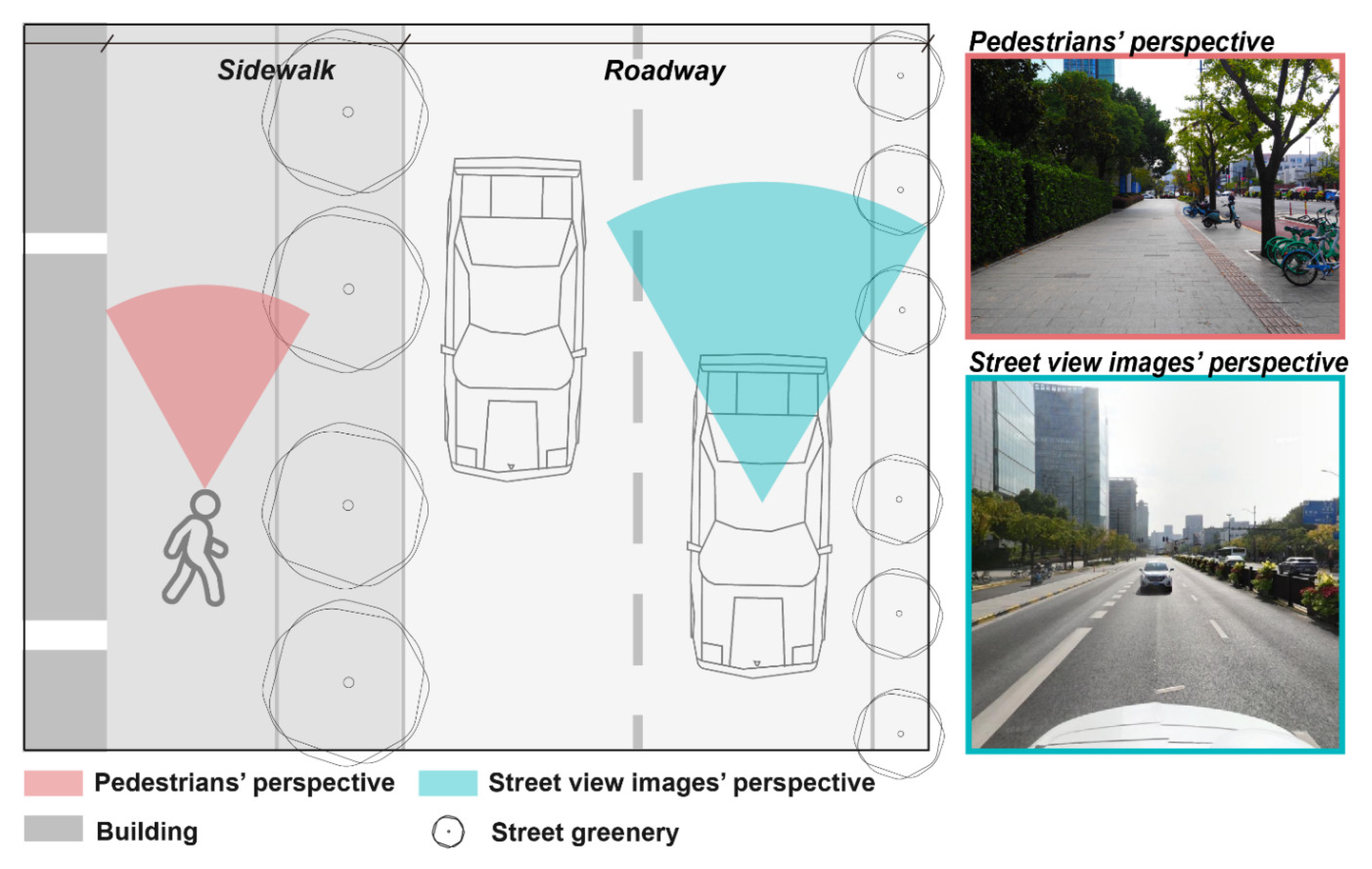
However, how street view image-based GVI (GVI_SVI) aligns with pedestrians’ perspective remains unknown and related influencing factors have not been examined. Moreover, the differences in GVI_SVI extracted from different kinds of street view image (SVI) have not been examined. SVI is usually collected by automobiles on motor lanes with a distance from sidewalks, and may have a different field of view than pedestrians’ perspective (
Figure 1). The vertical difference between the camera height of street view images and pedestrians’ eye level also contributed to such a difference. For instance, a research conducted in Singapore found that street view images do not have a high enough correlation with photos taken on road shoulder or sidewalks [
7]. Moreover, comparisons of different approaches in obtaining street view images have not been conducted, and related influencing factors have not been identified. These gaps may constrain the effective utilization of street view images in more urban environment studies.
Responding to the above-mentioned neglect, the present study tries to compare the GVI_SVI using different SVI (60° field of view, 90° field of view, panoramic) to GVI based on on-site photos imitating pedestrians’ perspective. Moreover, factors that may influence GVI_SVI have been explored, including road type, level of greenery and the interaction of the two factors. The research enables a comparison of GVI_SVI across different street view images and their alignments with the pedestrian-perceived greenery, and provide empirical findings from Shanghai. The study could contribute to the improvement in processing street view images, and thus finally promote the application of street view images in urban studies.
2. Literature Review
2.1. Green View Index Is Crucial in Measuring Urban Greenery Perception
Two kinds of variables were widely used to objectively evaluate urban greenery, including the ones addressing the distribution of greenspace from an overhead-view, and the ones measuring visible greenery from the human perspective [
9,
10]. Percentage of green space rate [
11,
12,
13], green coverage [
14,
15], normalized difference vegetation index (NDVI) [
15,
16,
17] are of the first groups of variables, which focus on the allocations of green space two-dimensionally. Green view index (GVI) belongs to the second group of measurements and addresses people’s visual experience [
10]. Extant studies suggested that GVI is not completely related to overhead-view indicators of green space, such as NDVI [
18,
19,
20,
21]. Moreover, overhead-view measurements of green spaces are less related to residents’ direct perception towards urban greenery [
15]. Green view index (GVI) measures urban greenery at eye-level, which refers to the proportion of plants in the entire field of view when observing on the ground [
22]. Visual information is crucial to influence people’s overall perception of the environment [
23]. Compared with overhead-view greenery measurements, GVI is more effective in obtaining people’s subjective perceptions of urban greenery level [
9].
2.2. High GVI Has Multiple Benefits
Existing research has proven that high level of GVI contributes to mental and physical health [
4,
5], perceived happiness [
6], physical activity [
24,
25,
26], better air condition [
27], and help reduce heat-mortality risk [
28]. A Japanese study found people who could see greenery from a room window experienced less depression and had higher life satisfaction and subjective happiness during the COVID-19 pandemic [
4]. People exposed to high levels of street GVI are more likely to report they have a good health condition [
5]. A total of 35% to 45% GVI is linked to higher perceived happiness [
6]. In a study involving 1390 residents in Hong Kong, researchers found that people who live on streets with higher GVI have a higher level of physical activity [
24]. High eye-level greenery in working places is also shown to be related to more recreational walking [
25]. A study involving time-series data between 2005 and 2018 in Hongkong found that high eye-level street greenery is associated with lower heat-mortality risk, since vegetation may improve microclimate by evapotranspiration [
28].
2.3. Measuring GVI Using Different Kinds of Street View Images
Street view images have been the most important data source to measure GVI and have been widely used in recent years [
2,
29]. The most frequently used street view images include Google Street View [
30,
31,
32,
33], Baidu street view [
34,
35,
36] and Tencent Map [
37]. Integrated platforms to process street view images have been established [
38,
39], and exploring how human beings perceive urban environments has become more and more important [
40,
41]. Street view images usually have five parameters, including picture size, location, heading, field of view (FOV), and pitch [
30]. Size refers to the image size of the street view images, location has the information of the latitude and longitude, and heading means the horizontal angle of the camera (0–360°). Field of view is the angle of the view the camera can capture. Pitch represents the vertical angle of the camera when taking the street view images, and is usually set as 0°.
By setting the above parameters with different values, researchers can obtain different street view images of the same point for GVI calculation. Generally, four-direction images and panoramic images are the two main kinds of images that are usually applied. For the four-directions images, the heading parameter is set as 0°, 90°, 180° and 270°, and four separate images facing front, right, back, and left could be acquired [
33,
37,
42]. Researchers usually set the field of view as 90° [
33,
43]. For panoramic street view images, researchers could set the field of view (FOV = 360°) to directly obtain panoramic images [
44], or stitch separate images facing different directions using the image stitch algorithm [
31]. For instance, in a study conducted in Japan, researchers created the 360° panoramic street view images based on 10 directions’ street view images [
30]. To alleviate the distortions at the ends of the panoramic image, some studies cropped square images in the center of the panoramic image to more accurately assess GVI [
32]. Parts of the panoramic images were also used to represent the left, front, and right fields of views of pedestrians by selecting the squared images in the middle [
32,
45].
3. Research Design and Methods
3.1. Study Site and Sample Points
We selected our sample points according to the availability of Baidu street view images in October 2022 to better compare with the on-site measured GVI. Street view images in 2022 were the latest street view images we could get. Baidu street view images cover most cities in China and have been widely used in green view index measurement [
34,
35,
36]. The southern part of Yangpu district, Shanghai, is our study site. Yangpu district is one of the central districts of Shanghai, with an area of 60.6 km
2 and 1.2 million people by the end of 2023. The population density in Yangpu district is around 19,800 people per km
2. We first obtained the street view images every 200 m along the streets in the southern part of Yangpu district using Baidu map API (Baidu, Inc., Beijing, China) The points which have street view images in October 2022 were selected as sampling points. Sample points were excluded if their street view images were incomplete, were taken on elevated roads or underground tunnels, contained significant obstructions (e.g., vehicles or fences), or showed signs of urban redevelopment or major environmental change.
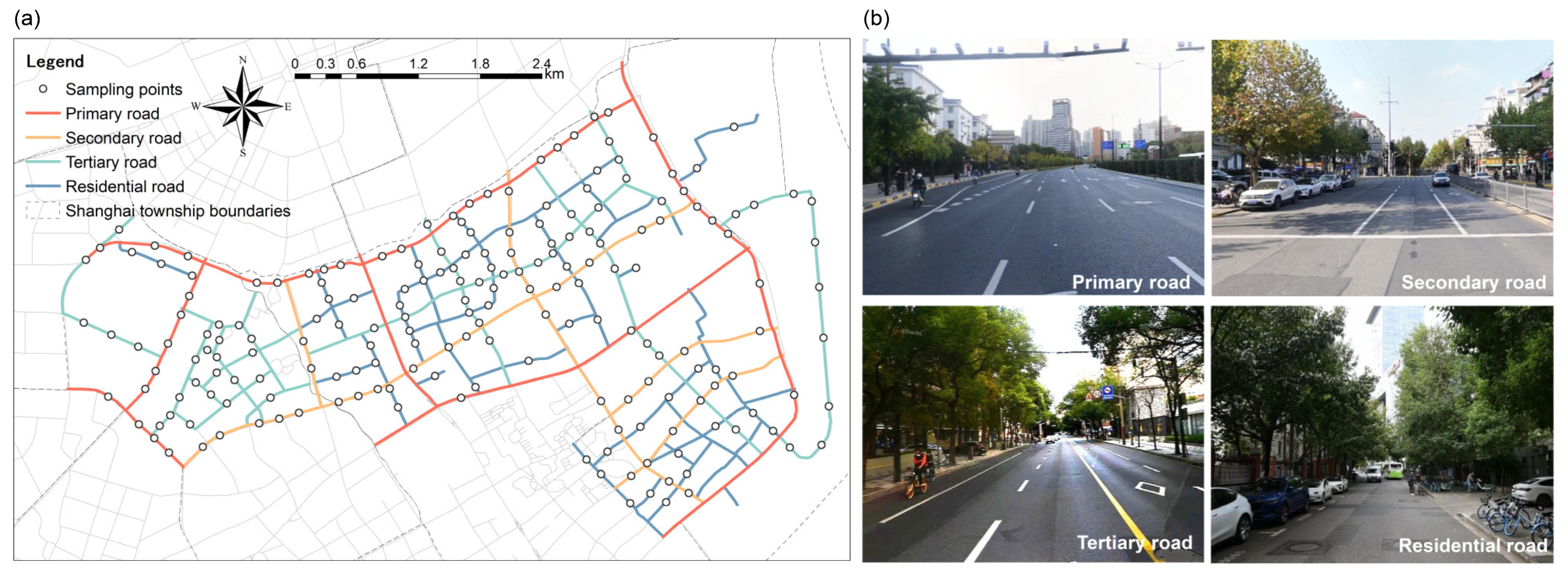
In total, 194 sample points on 68 streets were selected. These sample points were located on various kinds of streets, including 10 primary roads, 6 secondary roads, 24 tertiary roads, and 28 residential roads, according to the classification of Open Street Map (
https://wiki.openstreetmap.org/wiki/Template:Map_Features:highway, accessed on 8 October 2024). In our study site, the primary road refers to the main road with a width of 30–50 m, the secondary roads are around 20–30 m wide, tertiary roads are around 15–20 m wide, and residential roads are less than 15 m wide (
Figure 2). Specifically, the sample points are distributed across primary, secondary, tertiary, and residential roads with counts of 36, 37, 65, and 56, respectively. This stratified distribution ensures a representative sample set that includes different urban street typologies.
3.2. Measuring GVI_SVI Using SVI with Different Field of View
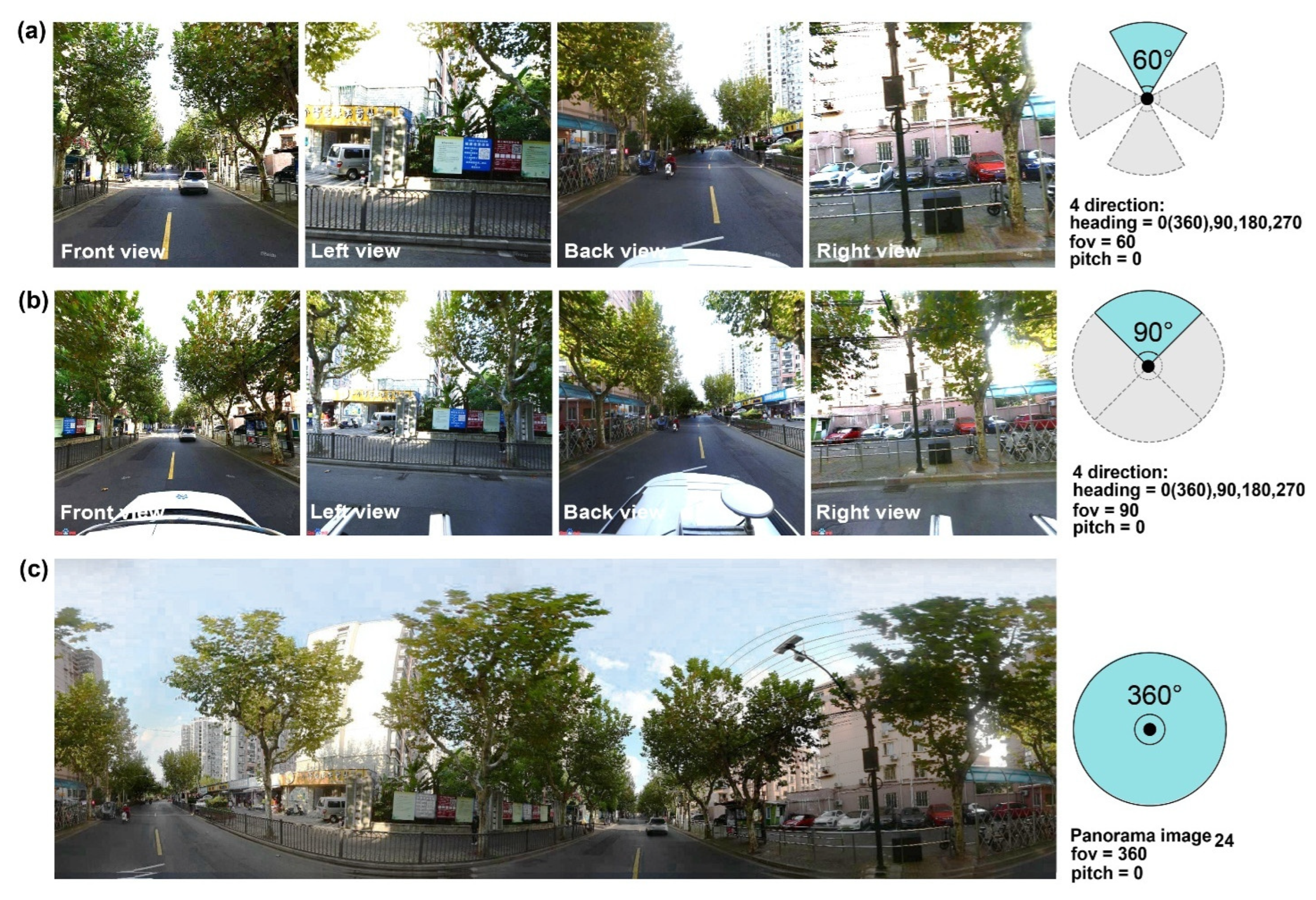
Three widely used approaches were applied to get the street view images of the same sample points, including four direction images with the field of view of 60°, four direction images with the field of view of 90°, and the panoramic images (
Figure 3). When the four direction images were obtained, the parameters of the headings were set as 0°, 90°, 180°, and 270°, respectively. To reduce edge distortion in the panoramic photos, the bottom of the images were cropped according to previous studies [
46]. We used DeepLabV3+ model pre-trained with ‘ADE20K’ dataset to segment street view images (
https://github.com/open-mmlab/mmsegmentation, accessed on 5 January 2025). DeepLabV3+ model is one of the most advanced deep learning models and has been widely applied in street view image segmentation [
30,
42,
47,
48]. Images of 20 sample points were randomly selected and manually annotated to compare with the segmentation results of DeepLabV3+ model. The average IoU of the vegetation was 0.839, which suggests that the segmentation results were reliable for GVI calculation. Then GVI based on the street view images with a field of view of 60° (GVI_SVI_60), 90° (GVI_SVI_90), and panoramic view (GVI_SVI_Pan) were calculated.
3.3. GVI Measured On-Site
We measured the on-site green view index from the pedestrians’ perspective based on on-site taken photos, which has been a widely used approach [
29,
49]. In the present study, pedestrians’ perspective refers to the eye-level visual environment perceived by pedestrians while walking on the sidewalk. We used on-site taken photos taken on sidewalks to imitate pedestrians’ perspective. For the on-site taken photos, the focal length is a critical parameter, as it directly determines the camera’s field of view, thereby affecting the extent to which the urban environment is captured in the image. A wider field of view can include the trees on the sides of the streets, while a narrow field of view may not be able to capture these trees. Thus, focal length is an important influencing factor in measuring on-site GVI. For most people, a view angle between 50 and 60° equals the central field of view, which is for color and spatial discrimination [
50], and is suitable for evaluating green view index. For full-frame cameras, a study in Japan found that photos taken with 28 mm focal length are the most suitable to evaluate street GVI, since the GVI obtained from these pictures are highly correlated with people’s on-site perceptions [
51]. Field of view angles between 50° and 60° have been widely used when obtaining on-site photos to analyze GVI [
22,
49,
52,
53]. In the present study, we used an OLYMPUS E-PL7-1442-EZ camera (Olympus Corporation, Tokyo, Japan) to take the photos of street sample points. It is a mirrorless interchangeable lens camera with a Four Thirds sensor. Following previous studies, we set the focal length to 17 mm, equivalent to a field of view of about 60°, to capture the central field of view and better approximate pedestrian’s perspective.
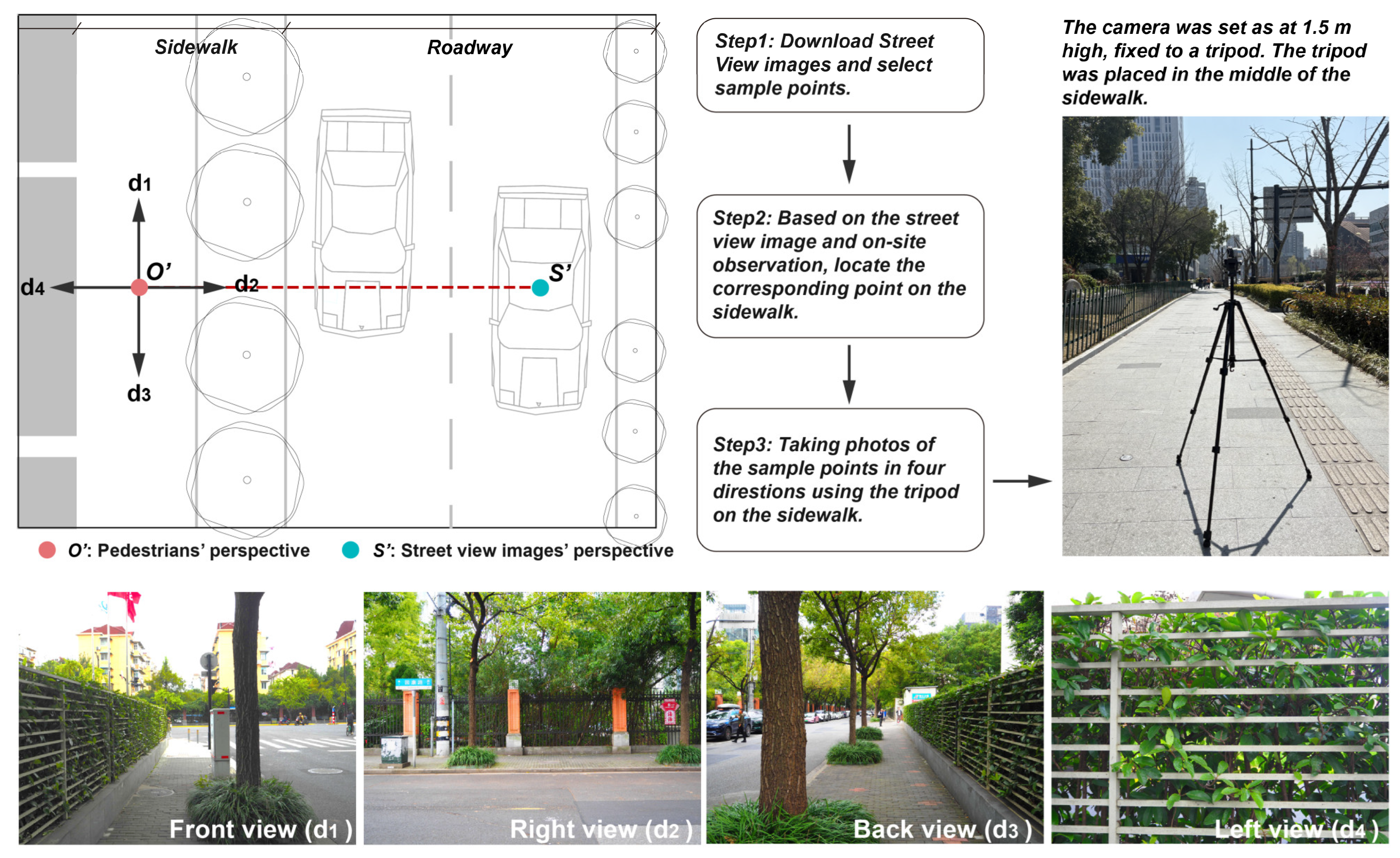
Researchers located the 194 sample points based on the Baidu street view images and in-person field confirmation (
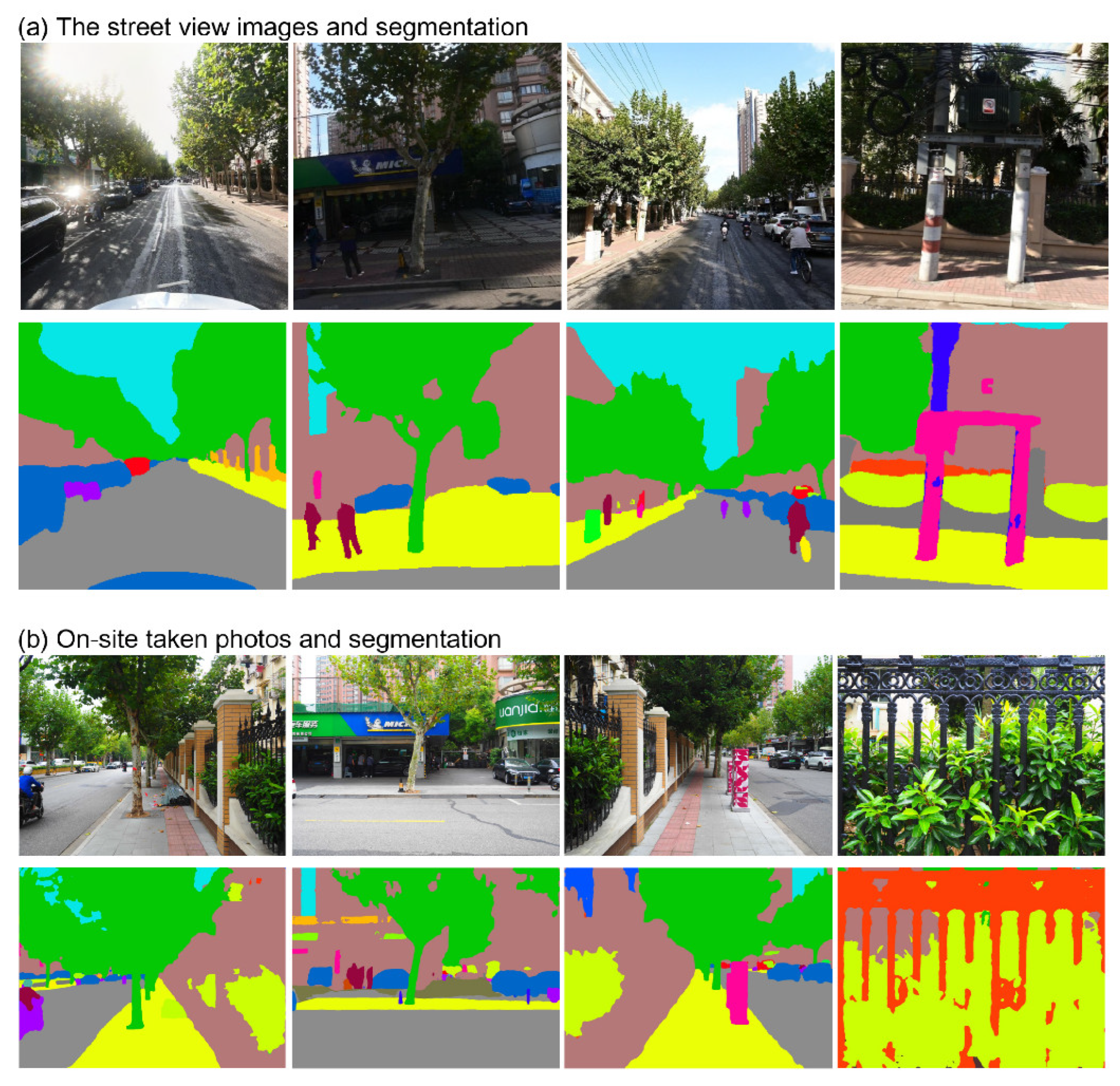
Figure 4). Four separate photos facing front, right, back, and left were taken for each sample point. The camera was set as at 1.5 m high, fixed to a tripod and placed in the middle of the sidewalk to imitate the perspective of pedestrians. Worked as one group, two trained graduate students took the photos of all the sample points together. We first took the photo of the sample points facing front, then rotated the camera 90° clockwise according to the angle on the tripod to take the photos facing right. Photos facing back and left were taken in the same manner. The size of each photo is 4608 × 3456 px. All the photos were taken on sunny or cloudy days, between 9:00 a.m. to 16:00 p.m. Moreover, to ensure the time of on-site taken photos is consistent with the time of street view images, all the on-site photos were taken in the October 2024. On-site taken photos were semantically segmented using the same model of DeepLabV3+ model as the street view images (
Figure 5).
3.4. Evaluating the Differences Between the GVI_SVI and Pedestrians’ Perception and Identify Influencing Factors
We quantified the differences between GVI_SVI and the GVI of pedestrians’ perception by comparing them with the GVI calculated using on-site taken photos. First, absolute error (AE), relative error (RE), mean square error (MSE), and mean absolute error (MAE) were computed. These are the most widely used variables to assess the difference in the measurement [
54,
55]. Then ANOVA analyses were used to explore whether the street type and greenery level may influence the performances of GVI_SVI computed.
AE measures the difference between what we observed and the true value [
55]. RE quantifies the proportion of the error to the true value [
56]. MSE is the average of the squared deviation of the estimator from the true value [
57]. A lower MSE indicates a smaller average squared difference. MAE measures the average of the absolute value of the difference between the observed and true value [
54].
AE is absolute error. RE is the relative error. MSE is the mean square error. MSE is squared deviation. MAE is the mean absolute error. GVI_SVI refers to the green view index measured based on street view images. GVI_OS is the GVI measured based on on-site-taken photos.
4. Results
4.1. Descriptive Statistics of GVI_SVI Using Different Approaches
In total, the green view indexes of 194 points were computed based on the on-site-taken photos (
Table 1). GVI calculated from on-site photographs (GVI_OS) is significantly related to GVI_SVI_60 (r = 0.648,
p < 0.01), GVI_SVI_90 (r = 0.592,
p < 0.01), and GVI_SVI_Pan (r = 0.497,
p < 0.01). Comparisons were made among GVI_OS and GVI_SVI obtained using different approaches. GVI_OS has a mean of 25.6%, which is similar compared to GVI_SVI_60 (25.3%), GVI_SVI_90 (23.1%), and GVI_SVI_Pan (26.8%). However, the minimum of GVI_OS (1.5%) is much larger than the minimum of GVI_SVI_60 (0.3%), GVI_SVI_90 (0.7%), and GVI_SVI_Pan (0.3%). The GVI_SVI_Pan has the largest standard deviation (17.2%), followed by GVI_OS (12.8%), GVI_SVI_90 (11.4%), and GVI_SVI_60 (11.3%).
4.2. Absolute Errors of GVI_SVI
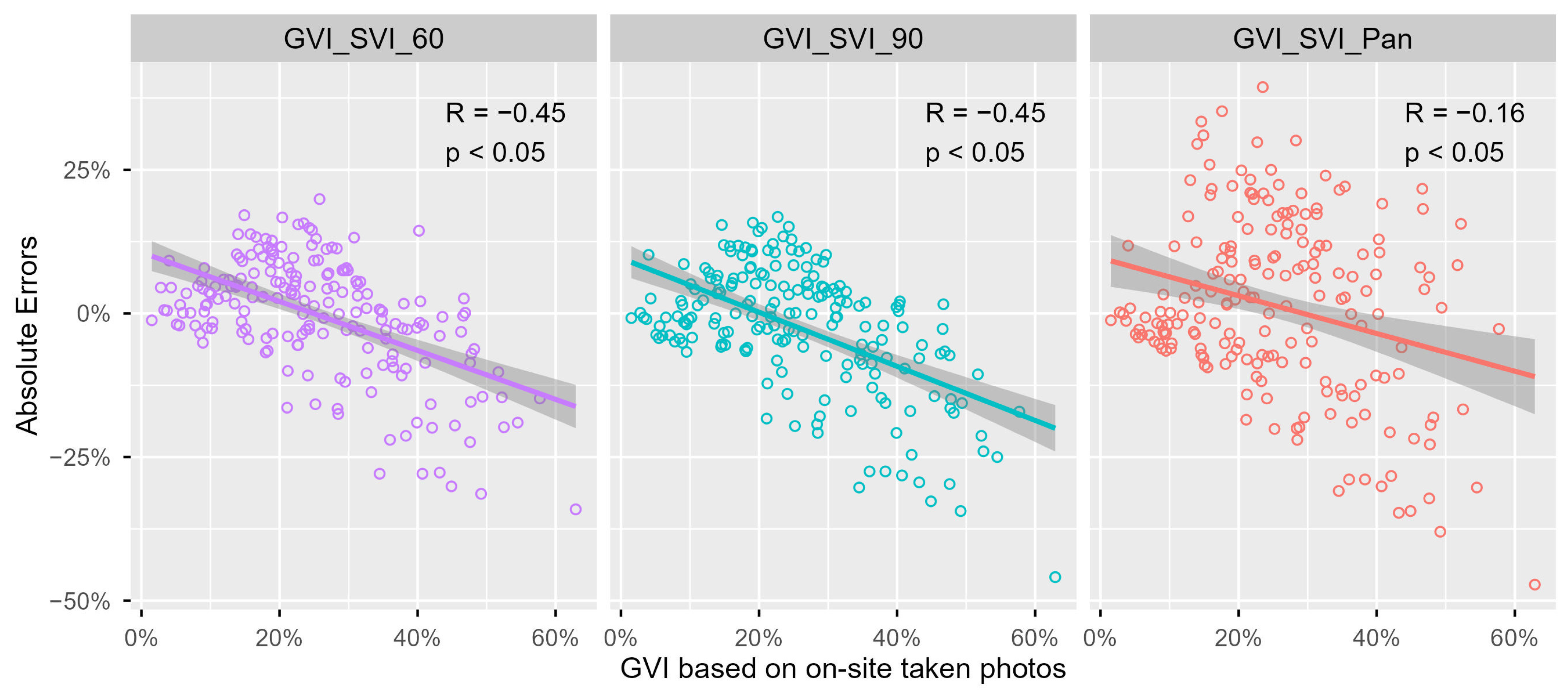
GVI_SVI_60 has the least absolute error, and GVI_SVI_Pan has the largest absolute error. The absolute error was calculated as GVI_SVI minus GVI_OS (
Table 2,
Figure 6). The proportions of absolute error smaller than −20% or larger than 20% for the GVI_SVI_60, GVI_SVI_90, and GVI_SVI_Pan are 4.64%, 7.74%, and 20.62%, respectively. For instance, for GVI_SVI_Pan, 16 (8.24%) sites have an absolute error smaller than −20%, and 24 (12.37%) sites have an absolute larger than 20%. The proportions of absolute error smaller than −10% or larger than 10% for the GVI_SVI_60, GVI_SVI_90, and GVI_SVI_Pan are 29.38%, 31.45%, and 49.48%, respectively. For instance, for GVI_SVI_90, 37 (19.07%) sites have an absolute error smaller than −10%, and 24 (12.37%) sites have an absolute error larger than 10%. The negative R values indicated a general tendency that the larger GVI_OS, the greater the underestimation of GVI by street view images.
4.3. The Relative Error of GVI_SVI
GVI_SVI_60 has the least relative error, while GVI_SVI_Pan has the largest one. We divided the absolute error of GVI_SVI by GVI_OS to measure the relative errors of GVI_SVI (
Table 3). The proportions of relative errors smaller than −40% or larger than 40% for GVI_SVI_60, GVI_SVI_90, and GVI_SVI_Pan are 34.54%, 35.57%, and 52.06%, respectively. The proportions of relative errors smaller than −60% or larger than 60% for GVI_SVI_60, GVI_SVI_90, and GVI_SVI_Pan are 16.50%, 17.53%, and 32.99%, respectively.
4.4. Mean Square Error and Mean Absolute Error of GVI_SVI
GVI_SVI_60 has the least mean square error and mean absolute error, which are 0.010 and 0.077, respectively. While GVI_SVI_Pan has the largest mean square error of 0.024 and the largest mean absolute error of 0.122. The mean square error and absolute error for GVI_SVI_90 are 0.013 and 0.082.
4.5. GVI_SVI of the Front View and Back View Are Closer to the Pedestrians’ Perspective
We compare the mean square error and mean absolute error of the front view and back views with those of left view and right views. Street view images were classified into two categories, including images of front and back views, and images of side (left and right) views. GVI_SVI for these two groups were calculated separately, and compared to GVI_OS in the front and back views as well as side views. The results indicated that for GVI_60, the mean square error and mean absolute error for the front and back views are 0.020 and 0.109, while the same measures for the side views are 0.034 and 0.134. For GVI_90, the mean square error and mean absolute error for the front and back views are 0.019 and 0.104, while the same measures for the side views are 0.038 and 0.144.
4.6. Road Type and Greenery Level in Relation to the Performance of GVI_SVI
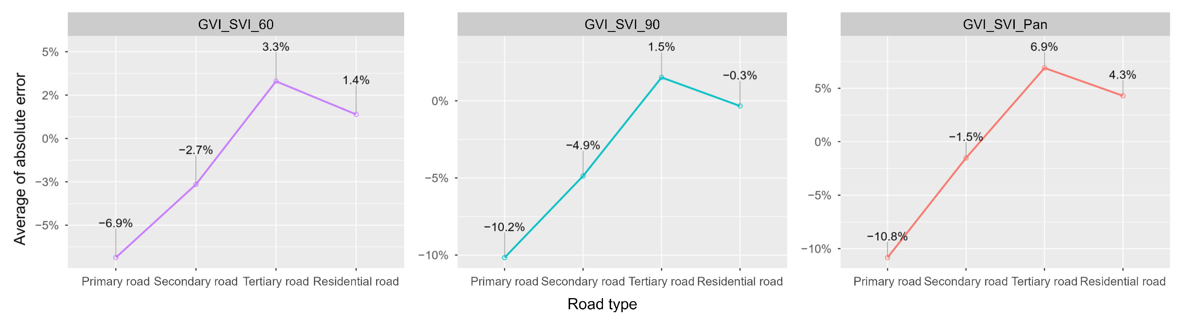
One-way ANOVA and two-way ANOVA analysis were utilized to explore the possible influences of road type and greenery level on the absolute error of GVI_SVI. One-way ANOVA indicated that compared to tertiary roads and residential roads, the errors of GVI_SVI for primary and secondary roads were significantly more negative, indicating stronger underestimation on wider roads (
Table 4,
Figure 7). Such a result indicated that GVI_SVI of the wide urban road significantly underestimated pedestrians’ GVI compared to narrow streets. For instance, for GVI_SVI_60, the mean absolute error of the primary road is −6.9%, and is significantly lower than that of tertiary road (
p < 0.001) and residential road (
p < 0.001). On the other hand, the mean absolute error of GVI_SVI of the residential roads is around 0, which indicates the GVI_SVI of this type of streets might better reflect pedestrians’ perception.
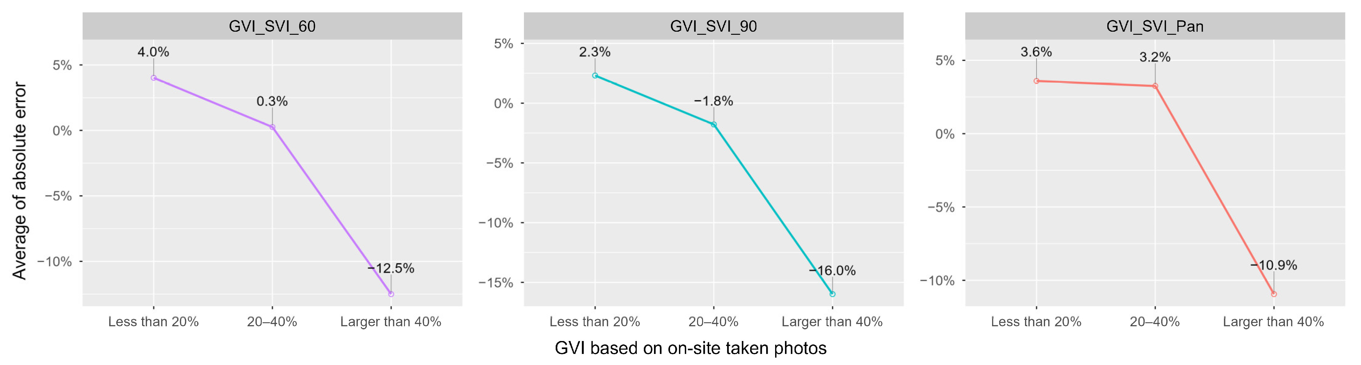
We further explored whether street greenery level influences the performance of GVI_SVI. Sample points were classified into three groups according to the GVI_OS, including the ones with GVI_OS less than 20%, 20–40%, and more than 40%. ANOVA analysis indicated that the absolute error of GVI_SVI is significantly smaller for the street with GVI_OS more than 40% (
Table 5,
Figure 8). Namely, GVI_SVI tends to underestimate the GVI of the streets with a high level of greenery. For instance, for GVI_SVI_60, the mean absolute errors for streets with greenery less than 20%, between 20 and 40%, and more than 40% are 4.0%, 0.3%, and −12.5%, respectively. The absolute error of streets with greenery more than 40% is significantly smaller than that with greenery less than 20% (
p < 0.001) and 20–40% (
p < 0.001).
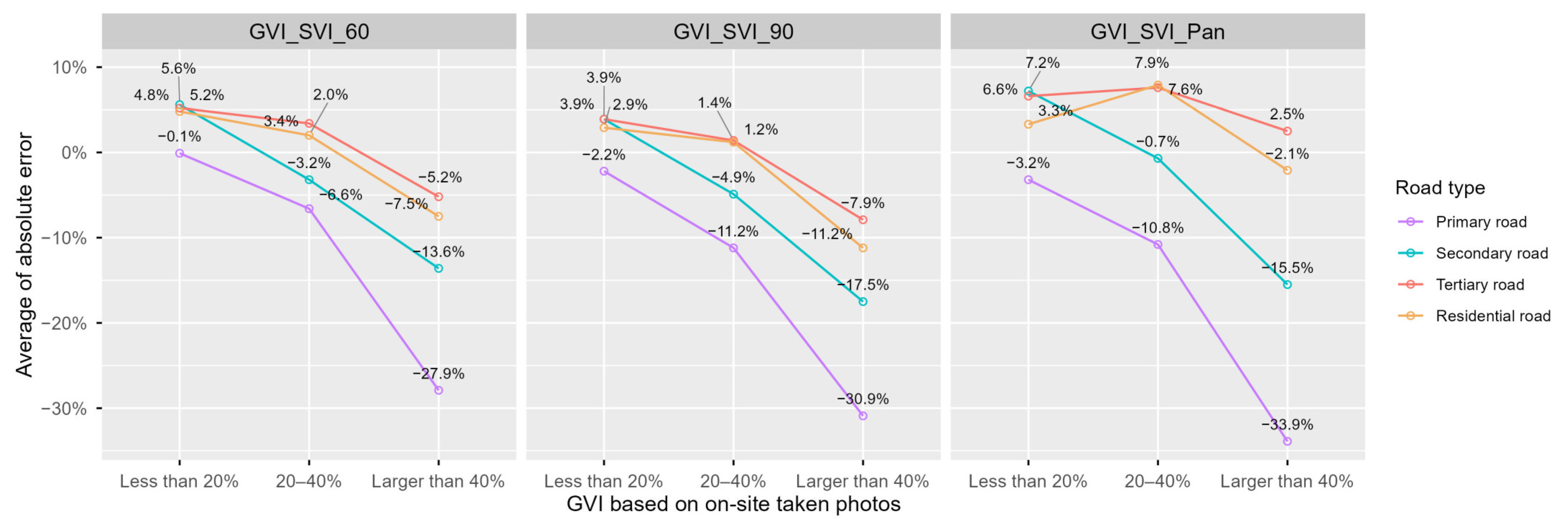
Two-way ANOVA analysis indicated that road type, and greenery degree collectively influence the performances of GVI_SVI calculated using all three kinds of SVI (
Figure 9,
Table 6). The interaction effect of street type and greenery level is also significant. The GVI of the primary road with more greenery is underestimated the most.
4.7. Using GVI_SVI_60 to Predict GVI from Pedestrians’ Perspective
We established a multiple linear regression model to explore how road type and measured GVI_SVI_60 are related to GVI_OS. For the model, GVI_OS is the dependent variable. Following the above classification, road type includes primary road, secondary road, tertiary road and residential road. GVI_SVI_60 are classified into less than 20%, 20–40%, and more than 40%. Both street type and GVI_SVI_60 were transferred into dummy variables. The result indicates that primary road type was positively significantly related to GVI_OS (
β = 0.188,
p = 0.004) (
Table 7). The overall R
2 for the model is 0.481, which has an acceptable explanatory power compared with similar studies [
58,
59].
5. Discussions
5.1. GVI_SVI Could Reflect Pedestrians’ Perspective and Images with a 60° Field of View Show the Closet Alignment with Pedestrians’ Perspective
Our result indicates that GVI_SVI is correlated with GVI captured from the perspective of pedestrians. Compared with GVI based on street view images with a 90° field of view and the panoramic images, the ones based on street view images with a 60° field of view have the least absolute error, relative error, mean square error, and absolute error. It indicates that street view images with a 60° field of view are more suitable to be applied when using GVI_SVI to measure GVI of pedestrians’ perspective. Existing research indicates that for human beings, the central field of view is within 50–60° of the view angle, which is the main view field to perceive color and form, and influences our visual perception the most [
50]. The sensitivity of color perception also decreases from the fovea to the periphery of the field of view [
60]. On-site photos were taken with a 60° field of view and are closer to GIV_SVI_60. Future study should explore more advanced methods to imitate pedestrians’ perspective and alleviate the potential bias related to field of view. On the other hand, panoramic images may exhibit pronounced distortion due to the spherical projection, which tends to result in larger differences between GVI_SVI_Pan and the GVI of pedestrians’ perspective [
61]. More research should be undertaken to further explore the differences in GVI calculated based on street view images with different fields of view and numbers of directions.
5.2. GVI_SVI for Front and Back Views Are More Accurate
Our study found that GVI_SVI of the front and back views have a smaller mean squared error and mean absolute error compared to those of the side views. Front view is the most important one that could influence our environment perception, since people always face the front when they walk [
62]. Plants and walls on the side may randomly influence the accuracy of GVI_SVI. For instance, if the point chosen has walls on the side, it may have a lower GVI compared with another point, even if these two points are on the same road and close to each other. One-direction normal photos are similar in representing the whole environment compared to on-site visits [
63], and have been widely used in environment perception studies [
64,
65]. Further research may examine the feasibility of using front- and back-view GVI to represent the street GVI from the perspective of pedestrians.
5.3. GVI_SVI Tends to Underestimate the GVI of Wide Roads
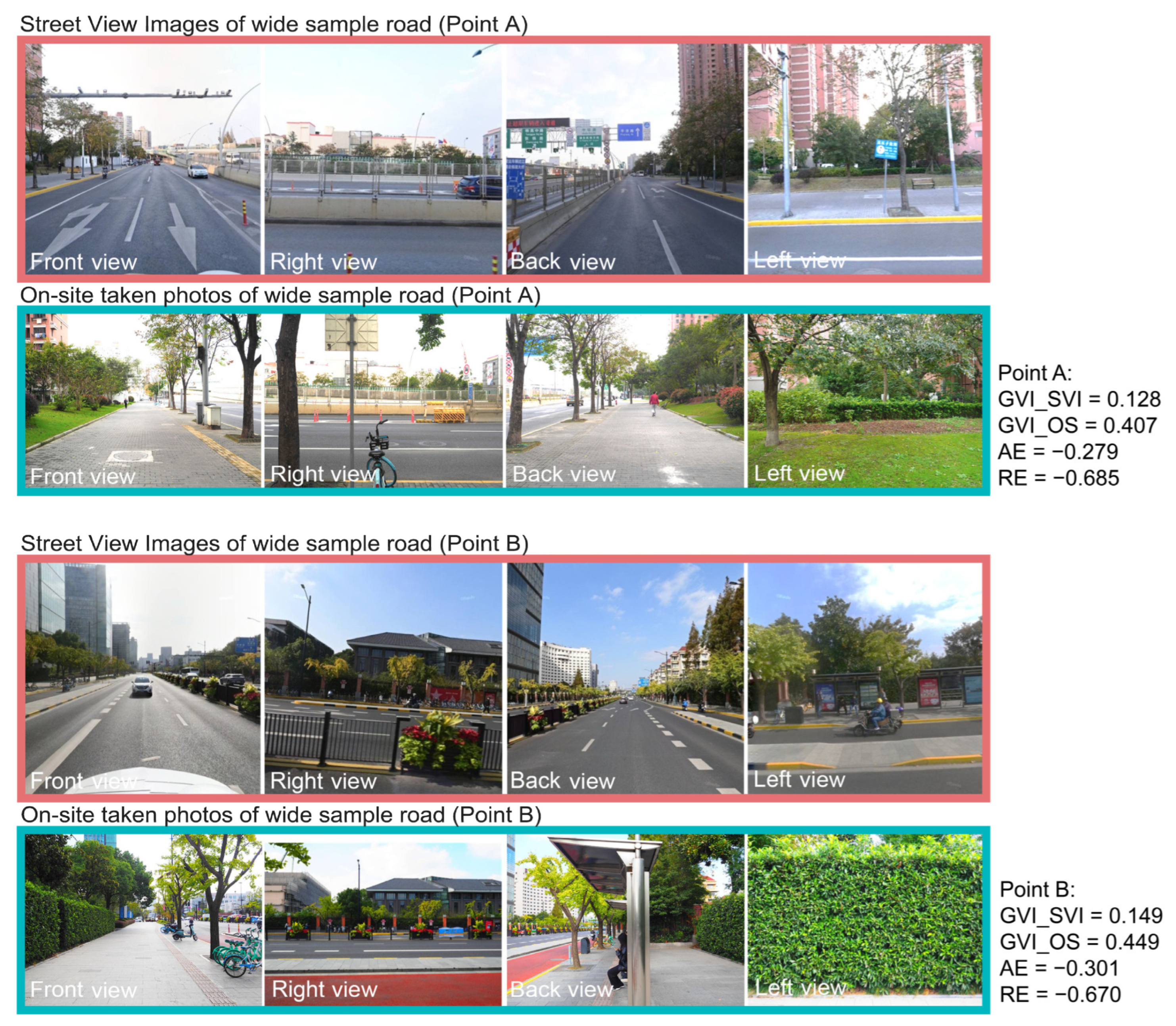
Our findings indicated that GVI of primary and secondary roads is significantly underestimated by GVI_SVI. That might be because these roads have a wider width. Specifically, roads under the elevated roads and roads above the underground tunnels are usually very wide. If the road is wide, the automobiles collecting the SVI might be in the mid-lanes of the road and are far away from the sidewalk, and hence may not capture the trees on sidewalks. At the same time, wide roads usually have wider sidewalks and more shrubs on the sidewalks, which cannot be seen from the car on the motorized lanes (
Figure 10). Such a result is consistent with the findings in the studies conducted in Singapore [
7] and Japan [
49], where researchers found wider road have a larger distance between the automobile lane and sidewalk, thus resulting in a larger discrepancy between street view images and pedestrian perspective.
5.4. GVI_SVI Tends to Underestimate the GVI of Roads with High Levels of Greenery
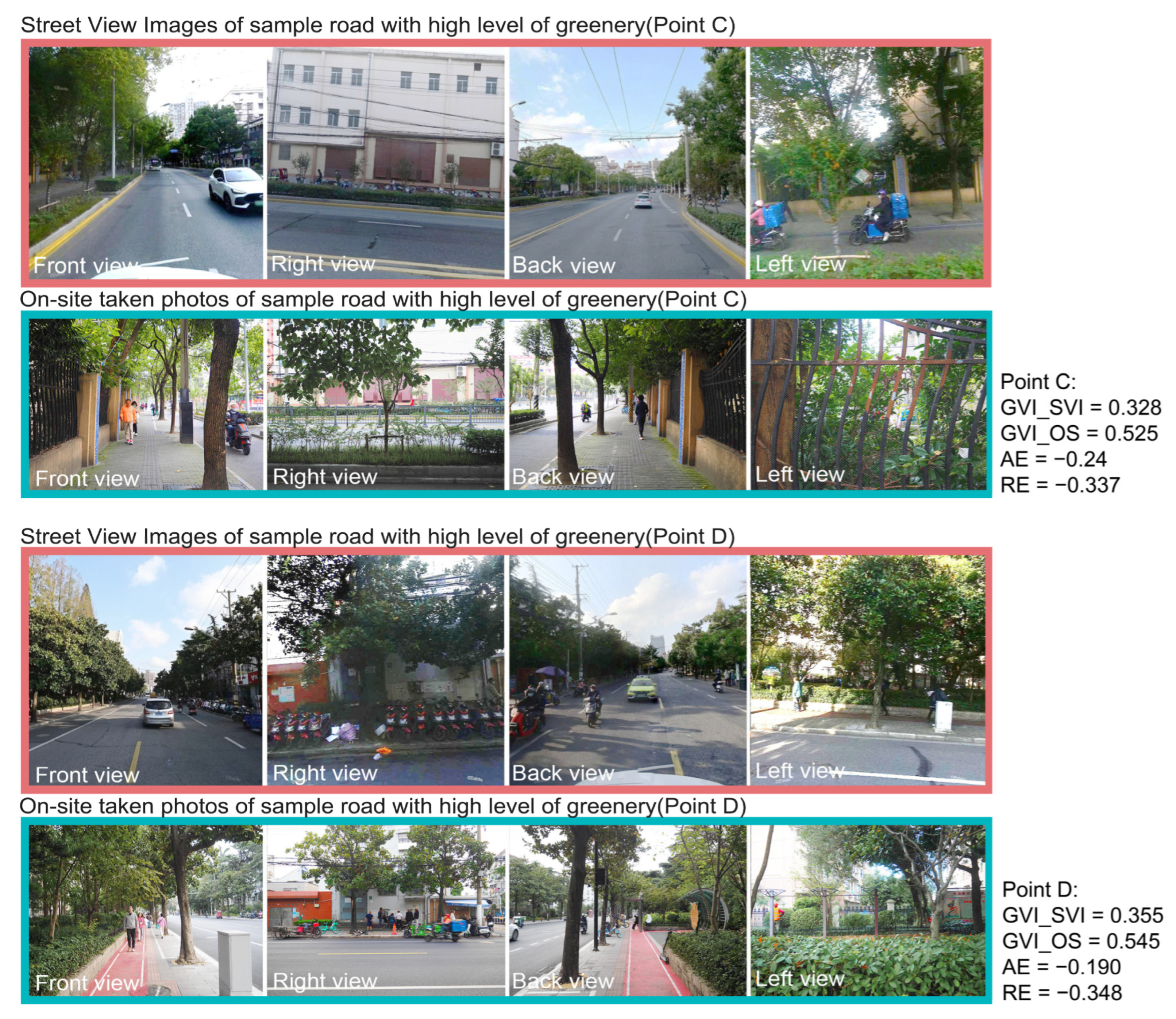
Our results indicate that GVI_SVI is more likely to underestimate the GVI of roads with more greenery. That might be because roads with abundant greenery often feature tiered planting designs on sidewalks, incorporating trees, shrubs, and grass. When walking on the sidewalks, people are close to the greenery (
Figure 11). Thus, these plants constitute a large proportion of pedestrians’ field of view. In contrast, the SVI camera may capture a larger part of buildings rather than the greenery when affiliated with the car on the motorized lanes.
5.5. Agreed Protocol Is Needed to Extract GVI from SVI
The present study indicates that GVI_SVI is significantly related to on-site measured GVI. However, agreed protocol is needed to improve the alignment between GVI_SVI and the pedestrians’ perception. The present study found that the proportions of the absolute error of GVI_SVI larger than 10% for the GVI_SVI_60, GVI_SVI_90, and GVI_SVI_Pan are 29.38%, 31.45%, and 49.48%. Such a result might be different from previous studies. In a study conducted in Japan, researchers found that GVI measured based on street view images is highly correlated with those measured using on-site taken photos [
49]. Among the 77 sites, 64 (83.12%) sites have the differences in green view index between street view images and on-site photos are less than ±5% [
49]. The contrast might be because all the roads had automobile lanes and sidewalk, and we took the photos on the sidewalk to imitate pedestrians’ field of view, and compared them with street view images captured from the roadway. In contrast, previous studies have many roads only with automobile lanes or sidewalks, which result in the same taken position of street view images and on-site photos.
An agreed approach has not been established to set crucial parameters in obtaining the street view images to calculate GVI. For instance, existing studies may use four-direction images [
33,
43], single panoramic images [
44], or stitched panoramic images [
30,
31] in assessing GVI. Issues of number of directions to obtain photos and the angle of view field have not been thoroughly discussed. Future research should explore how to set related parameters in order to improve the performance of GVI_SVI in capturing pedestrians’ perspective, and ultimately propose an applicable approach. Moreover, calibration of GVI_SVI compared to on-site GVI should also be conducted to find the determining factors that influence the performance of GVI_SVI.
6. Limitations and Strengths
This study has two main limitations which should be cautiously considered when interpreting the related findings. First, the sample size of 194 points on various types of streets may not be large enough compared to the tremendous amount of street view images. Future studies should include more sample points. Second, the street view images were taken in 2022, while the on-site photos were taken in 2024. However, the street view images in 2022 are the most recent street view images that we could get. While plant communities are not static over a two-year span, it is reasonable to explore the effects of the type of SVI, road types, and road greenery levels on GVI_SVI, since the impacts of these influencing factors are what we addressed rather than the absolute differences between GVI_SVI and that from pedestrians’ perspective. For the strengths, we took the photos in the middle of sidewalks at eye level, which could fully capture the view field of pedestrians, and provide solid data for comparison. Moreover, the on-site photos were taken in the same month as the street view images, which could make possible for the comparison and enhance the reliability of the result.
7. Conclusions and Implications
This study quantified the alignments between the green view index calculated using different street view images (GVI_SVI) (60° field of view, 90° field of view, panoramic) and pedestrians’ perception by comparing them to the GVI computed using on-site taken photos on sidewalks. The influences of road width and road greenery level are also examined in the comparison. We found that GVI_SVI could reflect pedestrians’ perceptions. GVI_SVI based on the SVI with a 60° field of view is most congruent with the pedestrians’ perspective imitated by photographs taken on sidewalks. GVI_SVI of the front and back views better capture pedestrians’ GVI perception than that of side views. GVI of streets with wide widths and higher levels of greenery are more likely to be underestimated by GVI_SVI. These results could help improve the application of street view images in measuring the GVI from pedestrian’s perspective, and are beneficial to the establishment of an agreed protocol in measuring GVI utilizing street view images as well as the application of street view image in urban analytics.
Author Contributions
Conceptualization, Y.Z., X.Z. and Y.X.; Methodology, Y.Z. and X.Z.; Software, X.Z.; Validation, Y.L. and J.Y.; Formal Analysis, X.Z.; Investigation, X.Z. and Y.L.; Resources, Y.Z. and Y.X.; Data Curation, Y.L. and B.F.; Writing—Original Draft Preparation, Y.Z.; Writing—Review & Editing, Y.X.; Visualization, X.Z.; Supervision, Y.X.; Project Administration, Y.Z.; Funding Acquisition, Y.Z. All authors have read and agreed to the published version of the manuscript.
Funding
This research was funded by the National Natural Science Foundation of China, grant number 32471947 and Shaanxi Provincial Science and Technology Plan Project, grant number 2025JC-YBMS-486.
Data Availability Statement
The data presented in this study are available on request from the corresponding author due to privacy restrictions.
Conflicts of Interest
The authors declare no conflicts of interest.
References
- Larkin, A.; Gu, X.; Chen, L.; Hystad, P. Predicting perceptions of the built environment using GIS, satellite and street view image approaches. Landsc. Urban Plan. 2021, 216, 104257. [Google Scholar] [CrossRef] [Scilit]
- Biljecki, F.; Ito, K. Street view imagery in urban analytics and GIS: A review. Landsc. Urban Plan. 2021, 215, 104217. [Google Scholar] [CrossRef] [Scilit]
- Xiao, Y.; Tang, Y.; Li, H.; He, S. Examining state-led gentrification using street view imagery: Evidence from Shanghai, China. Cities 2026, 175, 107113. [Google Scholar] [CrossRef] [Scilit]
- Soga, M.; Evans, M.J.; Tsuchiya, K.; Fukano, Y. A room with a green view: The importance of nearby nature for mental health during the COVID-19 pandemic. Ecol. Appl. 2021, 31, e2248. [Google Scholar] [CrossRef] [Scilit] [PubMed]
- O’Regan, A.C.; Hunter, R.F.; Nyhan, M.M. “Biophilic Cities”: Quantifying the Impact of Google Street View-Derived Greenspace Exposures on Socioeconomic Factors and Self-Reported Health. Environ. Sci. Technol. 2021, 55, 9063–9073. [Google Scholar] [PubMed]
- Navarrete-Hernandez, P.; Kiarostami, N.; Yang, D.; Ozcakir, A. Green Enough? A dose-response curve of the impact of street greenery levels and types on perceived happiness. Landsc. Urban Plan. 2024, 251, 105130. [Google Scholar] [CrossRef] [Scilit]
- Ito, K.; Quintana, M.; Han, X.; Zimmermann, R.; Biljecki, F. Translating street view imagery to correct perspectives to enhance bikeability and walkability studies. Int. J. Geogr. Inf. Sci. 2024, 38, 2514–2544. [Google Scholar] [CrossRef] [Scilit]
- Xiao, Y.; Song, M. How are urban design qualities associated with perceived walkability? An AI approach using street view images and deep learning. Int. J. Urban Sci. 2025, 29, 66–91. [Google Scholar]
- Falfán, I.; Muñoz-Robles, C.A.; Bonilla-Moheno, M.; MacGregor-Fors, I. Can you really see ‘green’? Assessing physical and self-reported measurements of urban greenery. Urban For. Urban Green. 2018, 36, 13–21. [Google Scholar] [CrossRef] [Scilit]
- Torkko, J.; Poom, A.; Willberg, E.; Toivonen, T. How to best map greenery from a human perspective? Comparing computational measurements with human perception. Front. Sustain. Cities 2023, 5, 1160995. [Google Scholar] [CrossRef] [Scilit]
- Zhang, L.; Zhou, S.; Kwan, M.-P.; Shen, M. Assessing individual environmental exposure derived from the spatiotemporal behavior context and its impacts on mental health. Health Place 2021, 71, 102655. [Google Scholar] [CrossRef] [Scilit]
- Zhou, X.; Wang, Y.-C. Spatial–temporal dynamics of urban green space in response to rapid urbanization and greening policies. Landsc. Urban Plan. 2011, 100, 268–277. [Google Scholar] [CrossRef] [Scilit]
- Sit, K.Y.; Chen, W.Y.; Ng, K.Y.; Koh, K.; Zhang, H. Unveiling environmental inequalities in high-density Asian city: City-scaled comparative analysis of green space coverage within 10-minute walk from private, public, and rural housing. Landsc. Urban Plan. 2025, 253, 105225. [Google Scholar] [CrossRef] [Scilit]
- Kanniah, K.D. Quantifying green cover change for sustainable urban planning: A case of Kuala Lumpur, Malaysia. Urban For. Urban Green. 2017, 27, 287–304. [Google Scholar] [CrossRef] [Scilit]
- Girma, Y.; Terefe, H.; Pauleit, S.; Kindu, M. Urban green spaces supply in rapidly urbanizing countries: The case of Sebeta Town, Ethiopia. Remote Sens. Appl. Soc. Environ. 2019, 13, 138–149. [Google Scholar] [CrossRef] [Scilit]
- Mennis, J.; Mason, M.; Ambrus, A. Urban greenspace is associated with reduced psychological stress among adolescents: A Geographic Ecological Momentary Assessment (GEMA) analysis of activity space. Landsc. Urban Plan. 2018, 174, 1–9. [Google Scholar] [CrossRef] [Scilit]
- Klein, R.; Willberg, E.; Korpilo, S.; Toivonen, T. Temporal variation in travel greenery across 86 cities in Europe. Urban For. Urban Green. 2024, 102, 128566. [Google Scholar] [CrossRef] [Scilit]
- Li, T.; Zheng, X.; Wu, J.; Zhang, Y.; Fu, X.; Deng, H. Spatial relationship between green view index and normalized differential vegetation index within the Sixth Ring Road of Beijing. Urban For. Urban Green. 2021, 62, 127153. [Google Scholar] [CrossRef] [Scilit]
- Huang, Y.; Sanatani, R.P.; Liu, C.; Kang, Y.; Zhang, F.; Liu, Y.; Duarte, F.; Ratti, C. No “true” greenery: Deciphering the bias of satellite and street view imagery in urban greenery measurement. Build. Environ. 2025, 269, 112395. [Google Scholar] [CrossRef] [Scilit]
- Larkin, A.; Hystad, P. Evaluating street view exposure measures of visible green space for health research. J. Expo. Sci. Environ. Epidemiol. 2019, 29, 447–456. [Google Scholar] [CrossRef] [Scilit]
- Helbich, M.; Poppe, R.; Oberski, D.; Zeylmans van Emmichoven, M.; Schram, R. Can’t see the wood for the trees? An assessment of street view- and satellite-derived greenness measures in relation to mental health. Landsc. Urban Plan. 2021, 214, 104181. [Google Scholar] [CrossRef] [Scilit]
- Yang, J.; Zhao, L.; McBride, J.; Gong, P. Can you see green? Assessing the visibility of urban forests in cities. Landsc. Urban Plan. 2009, 91, 97–104. [Google Scholar] [CrossRef] [Scilit]
- Gibson, J.J. The Ecological Approach to Visual Perception; Houghton Mifflin: Boston, MA, USA, 1979. [Google Scholar]
- Lu, Y. Using Google Street View to investigate the association between street greenery and physical activity. Landsc. Urban Plan. 2019, 191, 103435. [Google Scholar] [CrossRef] [Scilit]
- Yang, H.; Zhang, Q.; Helbich, M.; Lu, Y.; He, D.; Ettema, D.; Chen, L. Examining non-linear associations between built environments around workplace and adults’ walking behaviour in Shanghai, China. Transp. Res. Part A Policy Pract. 2022, 155, 234–246. [Google Scholar] [CrossRef] [Scilit]
- Lu, Y.; Sarkar, C.; Xiao, Y. The effect of street-level greenery on walking behavior: Evidence from Hong Kong. Soc. Sci. Med. 2018, 208, 41–49. [Google Scholar] [CrossRef] [Scilit]
- Sabedotti, M.E.; O’Regan, A.C.; Nyhan, M.M. Data Insights for Sustainable Cities: Associations between Google Street View-Derived Urban Greenspace and Google Air View-Derived Pollution Levels. Environ. Sci. Technol. 2023, 57, 19637–19648. [Google Scholar]
- Song, J.; Gasparrini, A.; Fischer, T.; Hu, K.; Lu, Y. Effect Modifications of Overhead-View and Eye-Level Urban Greenery on Heat–Mortality Associations: Small-Area Analyses Using Case Time Series Design and Different Greenery Measurements. Environ. Health Perspect. 2023, 131, 097007. [Google Scholar] [CrossRef] [Scilit] [PubMed]
- Yan, J.; Huang, X.; Wang, S.; He, Y.; Li, X.; Hohl, A.; Li, X.; Aly, M.; Lin, B. Toward a comprehensive understanding of eye-level urban greenness: A systematic review. Int. J. Digit. Earth 2023, 16, 4769–4789. [Google Scholar] [CrossRef] [Scilit]
- Xia, Y.; Yabuki, N.; Fukuda, T. Development of a system for assessing the quality of urban street-level greenery using street view images and deep learning. Urban For. Urban Green. 2021, 59, 126995. [Google Scholar] [CrossRef] [Scilit]
- Wang, J.; Liu, W.; Gou, A. Numerical characteristics and spatial distribution of panoramic Street Green View index based on SegNet semantic segmentation in Savannah. Urban For. Urban Green. 2022, 69, 127488. [Google Scholar] [CrossRef] [Scilit]
- Yin, L.; Cheng, Q.; Wang, Z.; Shao, Z. ‘Big data’ for pedestrian volume: Exploring the use of Google Street View images for pedestrian counts. Appl. Geogr. 2015, 63, 337–345. [Google Scholar] [CrossRef] [Scilit]
- Lu, Y.; Yang, Y.; Sun, G.; Gou, Z. Associations between overhead-view and eye-level urban greenness and cycling behaviors. Cities 2019, 88, 10–18. [Google Scholar] [CrossRef] [Scilit]
- Zhang, W.; Zeng, H. Spatial differentiation characteristics and influencing factors of the green view index in urban areas based on street view images: A case study of Futian District, Shenzhen, China. Urban For. Urban Green. 2024, 93, 128219. [Google Scholar] [CrossRef] [Scilit]
- Yu, X.; Her, Y.; Huo, W.; Chen, G.; Qi, W. Spatio-temporal monitoring of urban street-side vegetation greenery using Baidu Street View images. Urban For. Urban Green. 2022, 73, 127617. [Google Scholar] [CrossRef] [Scilit]
- Sun, L.; Wang, J.; Xie, Z.; Li, R.; Wu, X.; Wu, Y. Evaluating the Street Greening with the Multiview Data Fusion. J. Sens. 2021, 2021, 2793474. [Google Scholar] [CrossRef] [Scilit]
- Wang, R.; Lu, Y.; Zhang, J.; Liu, P.; Yao, Y.; Liu, Y. The relationship between visual enclosure for neighbourhood street walkability and elders’ mental health in China: Using street view images. J. Transp. Health 2019, 13, 90–102. [Google Scholar] [CrossRef] [Scilit]
- Ito, K.; Zhu, Y.; Abdelrahman, M.; Liang, X.; Fan, Z.; Hou, Y.; Zhao, T.; Ma, R.; Fujiwara, K.; Ouyang, J. ZenSVI: An open-source software for the integrated acquisition, processing and analysis of street view imagery towards scalable urban science. Comput. Environ. Urban Syst. 2025, 119, 102283. [Google Scholar] [CrossRef] [Scilit]
- Vartholomaios, A.; Lagarias, A. Mapping Urban Segregation with GeoAI: Street View Perceptions and Socio-Spatial Inequality in Thessaloniki, Greece. Land 2025, 14, 2083. [Google Scholar] [CrossRef] [Scilit]
- Dubey, A.; Naik, N.; Parikh, D.; Raskar, R.; Hidalgo, C.A. Deep learning the city: Quantifying urban perception at a global scale. In Proceedings of the European Conference on Computer Vision; Springer: Berlin/Heidelberg, Germany, 2016; pp. 196–212. [Google Scholar]
- Lou, S.; Stancato, G.; Boffi, M.; Rainisio, N.; Ceravolo, P.; Piga, B.E. Evaluating urban perception: Comparing Place Pulse 2.0 dataset results with images of varied field of view. In Misura/Dismisura| Measure/Out of Measure; Franco Angeli: Milan, Italy, 2024; pp. 471–482. [Google Scholar]
- Yang, W.; Li, Y.; Liu, Y.; Fan, P.; Yue, W. Environmental factors for outdoor jogging in Beijing: Insights from using explainable spatial machine learning and massive trajectory data. Landsc. Urban Plan. 2024, 243, 104969. [Google Scholar] [CrossRef] [Scilit]
- Seiferling, I.; Naik, N.; Ratti, C.; Proulx, R. Green streets− Quantifying and mapping urban trees with street-level imagery and computer vision. Landsc. Urban Plan. 2017, 165, 93–101. [Google Scholar] [CrossRef] [Scilit]
- Gao, J.; Ma, S.; Wang, L.; Shuai, L.; Du, H. Does greenness bring more green travelling? Evidence from free-floating bike-sharing in Beijing. J. Transp. Geogr. 2023, 109, 103586. [Google Scholar] [CrossRef] [Scilit]
- Ki, D.; Lee, S. Analyzing the effects of Green View Index of neighborhood streets on walking time using Google Street View and deep learning. Landsc. Urban Plan. 2021, 205, 103920. [Google Scholar] [CrossRef] [Scilit]
- Huang, G.; Yu, Y.; Lyu, M.; Sun, D.; Zeng, Q.; Bart, D. Using google street view panoramas to investigate the influence of urban coastal street environment on visual walkability. Environ. Res. Commun. 2023, 5, 065017. [Google Scholar] [CrossRef] [Scilit]
- Hipp, J.R.; Lee, S.; Ki, D.; Kim, J.H. Measuring the Built Environment with Google Street View and Machine Learning: Consequences for Crime on Street Segments. J. Quant. Criminol. 2022, 38, 537–565. [Google Scholar] [CrossRef] [Scilit]
- Kim, J.H.; Ki, D.; Osutei, N.; Lee, S.; Hipp, J.R. Beyond visual inspection: Capturing neighborhood dynamics with historical Google Street View and deep learning-based semantic segmentation. J. Geogr. Syst. 2024, 26, 541–564. [Google Scholar] [CrossRef] [Scilit]
- Aikoh, T.; Homma, R.; Abe, Y. Comparing conventional manual measurement of the green view index with modern automatic methods using google street view and semantic segmentation. Urban For. Urban Green. 2023, 80, 127845. [Google Scholar] [CrossRef] [Scilit]
- Torrejon, A.; Callaghan, V.; Hagras, H. Panoramic Audio and Video: Towards an Immersive Learning Experience. In Proceedings of the iED Europe Summit—London 2013, London, UK, 28–29 November 2013. [Google Scholar]
- Aoki, Y.; Yasuoka, Y.; Naito, M. Assessing the impression of street-side greenery. Landsc. Res. 1985, 10, 9–13. [Google Scholar] [CrossRef] [Scilit]
- Walker, H.K.; Hurst, J.W.; Hall, W.D. (Eds.) Visual Fields. In Clinical Methods: The History, Physical, and Laboratory Examinations; Butterworth Publishers: Boston, MA, USA, 1990. [Google Scholar]
- Li, X.; Zhang, C.; Li, W.; Ricard, R.; Meng, Q.; Zhang, W. Assessing street-level urban greenery using Google Street View and a modified green view index. Urban For. Urban Green. 2015, 14, 675–685. [Google Scholar] [CrossRef] [Scilit]
- Belyadi, H.; Haghighat, A. Chapter 5—Supervised learning. In Machine Learning Guide for Oil and Gas Using Python; Belyadi, H., Haghighat, A., Eds.; Gulf Professional Publishing: Houston, TX, USA, 2021; pp. 169–295. [Google Scholar]
- Shcherbakov, M.V.; Brebels, A.; Shcherbakova, N.L.; Tyukov, A.P.; Janovsky, T.A.; Kamaev, V.A.e. A survey of forecast error measures. World Appl. Sci. J. 2013, 24, 171–176. [Google Scholar]
- Jackson, E.K.; Roberts, W.; Nelsen, B.; Williams, G.P.; Nelson, E.J.; Ames, D.P. Introductory overview: Error metrics for hydrologic modelling—A review of common practices and an open source library to facilitate use and adoption. Environ. Model. Softw. 2019, 119, 32–48. [Google Scholar] [CrossRef] [Scilit]
- Schluchter, M.D. Mean square error. Encycl. Biostat. 2005, 5. [Google Scholar]
- Xie, X.; Zhou, H.; Gou, Z. Dynamic real-time individual green space exposure indices and the relationship with static green space exposure indices: A study in Shenzhen. Ecol. Indic. 2023, 154, 110557. [Google Scholar] [CrossRef] [Scilit]
- Lin, W.; Güneralp, B. Influence of urban-form and sociodemographic factors on street tree abundance transpire across scales in Houston, TX. Urban For. Urban Green. 2024, 94, 128263. [Google Scholar] [CrossRef] [Scilit]
- Hansen, T.; Pracejus, L.; Gegenfurtner, K.R. Color perception in the intermediate periphery of the visual field. J. Vis. 2009, 9, 26. [Google Scholar] [CrossRef] [Scilit] [PubMed]
- Lu, Y.; Ferranti, E.J.S.; Chapman, L.; Pfrang, C. Assessing urban greenery by harvesting street view data: A review. Urban For. Urban Green. 2023, 83, 127917. [Google Scholar] [CrossRef] [Scilit]
- Hollands, M.A.; Patla, A.E.; Vickers, J.N. “Look where you’re going!”: Gaze behaviour associated with maintaining and changing the direction of locomotion. Exp. Brain Res. 2002, 143, 221–230. [Google Scholar] [CrossRef] [Scilit]
- Stamps, A.E., III. Use of photographs to simulate environments: A meta-analysis. Percept. Mot. Ski. 1990, 71, 907–913. [Google Scholar] [CrossRef]
- Wilkie, S.; Stavridou, A. Influence of environmental preference and environment type congruence on judgments of restoration potential. Urban For. Urban Green. 2013, 12, 163–170. [Google Scholar] [CrossRef] [Scilit]
- Van Hecke, L.; Ghekiere, A.; Van Cauwenberg, J.; Veitch, J.; De Bourdeaudhuij, I.; Van Dyck, D.; Clarys, P.; Van De Weghe, N.; Deforche, B. Park characteristics preferred for adolescent park visitation and physical activity: A choice-based conjoint analysis using manipulated photographs. Landsc. Urban Plan. 2018, 178, 144–155. [Google Scholar] [CrossRef] [Scilit]
Figure 1.
Street view images may capture different fields of views compared to those of pedestrians.
Figure 1.
Street view images may capture different fields of views compared to those of pedestrians.
Figure 2.
Sample points distribution (a) and different types of roads (b).
Figure 2.
Sample points distribution (a) and different types of roads (b).
Figure 3.
Street view images of four direction with a 60° field of view (a), four directions with a 90° field of view (b), and the panoramic images (c).
Figure 3.
Street view images of four direction with a 60° field of view (a), four directions with a 90° field of view (b), and the panoramic images (c).
Figure 4.
Taking photos of sample points on sidewalks.
Figure 4.
Taking photos of sample points on sidewalks.
Figure 5.
Segmentation of street view images and on-site taken photos.
Figure 5.
Segmentation of street view images and on-site taken photos.
Figure 6.
Absolute error of GVI based on street view images.
Figure 6.
Absolute error of GVI based on street view images.
Figure 7.
One-way ANOVA analysis of absolute error of GVI_SVI and road type.
Figure 7.
One-way ANOVA analysis of absolute error of GVI_SVI and road type.
Figure 8.
One-way ANOVA analysis of absolute error of GVI_SVI and greenery level.
Figure 8.
One-way ANOVA analysis of absolute error of GVI_SVI and greenery level.
Figure 9.
Two-way ANOVA analysis of absolute error of GVI_SVI, road type and greenery level.
Figure 9.
Two-way ANOVA analysis of absolute error of GVI_SVI, road type and greenery level.
Figure 10.
Comparisons of wide roads’ street view images and on-site taken photos (Point A and Point B).
Figure 10.
Comparisons of wide roads’ street view images and on-site taken photos (Point A and Point B).
Figure 11.
Comparisons of street view images and on-site taken photos of roads with high levels of greenery (Point C and Point D).
Figure 11.
Comparisons of street view images and on-site taken photos of roads with high levels of greenery (Point C and Point D).
Table 1.
Descriptive statistics of GVI based on on-site taken photos and street view images.
Table 1.
Descriptive statistics of GVI based on on-site taken photos and street view images.
| | Range | Minimum | Maximum | Mean | Median | SD |
|---|
| GVI_OS | 61.4% | 1.5% | 62.9% | 25.6% | 24.3% | 12.8% |
| GVI_SVI_60 | 54.3% | 0.3% | 54.6% | 25.3% | 26.6% | 11.3% |
| GVI_SVI_90 | 47.6% | 0.7% | 48.3% | 23.1% | 24.0% | 11.4% |
| GVI_SVI_Pan | 68.0% | 0.3% | 68.3% | 26.8% | 24.6% | 17.2% |
Table 2.
Absolute error of GVI based on street view images.
Table 2.
Absolute error of GVI based on street view images.
| Absolute Error | GVI_SVI_60 | GVI_SVI_90 | GVI_SVI_Pan |
|---|
| <−40% | 0 (0%) | 1 (0.52%) | 1 (0.52%) |
| −40% to −30% | 3 (1.55%) | 3 (1.55%) | 7 (3.61%) |
| −30% to −20% | 6 (3.09%) | 11 (5.67%) | 8 (4.12%) |
| −20% to −10% | 21 (10.82%) | 22 (11.34%) | 23 (11.86%) |
| −10% to 0% | 55 (28.35%) | 68 (35.05%) | 54 (27.84%) |
| 0% to 10% | 82 (42.27%) | 65 (33.51%) | 44 (22.68%) |
| 10% to 20% | 27 (13.92%) | 24 (12.37%) | 33 (17.01%) |
| 20% to 30% | 0 (0%) | 0 (0%) | 19 (9.79%) |
| ≥30% | 0 (0%) | 0 (0%) | 5 (2.58%) |
Table 3.
Relative error of GVI based on street view images.
Table 3.
Relative error of GVI based on street view images.
| Relative Error | GVI_SVI_60 | GVI_SVI_90 | GVI_SVI_Pan |
|---|
| <−100% | 0 (0.00%) | 0 (0.00%) | 0 (0.00%) |
| −100% to −80% | 1 (0.52%) | 2 (1.03%) | 4 (2.06%) |
| −80% to −60% | 9 (4.64%) | 17 (8.76%) | 23 (11.86%) |
| −60% to −40% | 13 (6.70%) | 17 (8.76%) | 21 (10.82%) |
| −40% to −20% | 27 (13.92%) | 32 (16.49%) | 28 (14.43%) |
| −20% to 0% | 35 (18.04%) | 37 (19.07%) | 17 (8.76%) |
| 0% to 20% | 36 (18.56%) | 35 (18.04%) | 24 (12.37%) |
| 20% to 40% | 29 (14.95%) | 21 (10.82%) | 24 (12.37%) |
| 40% to 60% | 22 (11.34%) | 18 (9.28%) | 16 (8.25%) |
| 60% to 80% | 13 (6.70%) | 11 (5.67%) | 11 (5.67%) |
| 80% to 100% | 5 (2.58%) | 2 (1.03%) | 8 (4.12%) |
| ≥100% | 4 (2.06%) | 2 (1.03%) | 18 (9.28%) |
Table 4.
One-way ANOVA analysis of absolute error of GVI_SVI and road type.
Table 4.
One-way ANOVA analysis of absolute error of GVI_SVI and road type.
| | (I) Street Type | (J) Street Type | Mean Difference (I − J) | Std. Error | Sig. | 95% Confidence Interval |
|---|
| Lower Bound | Upper Bound |
|---|
| GVI_SVI_60 | Primary road | Secondary road | −4.2% | 2.2% | 0.061 | −8.6% | 0.2% |
| Tertiary road | −10.2% * | 2.0% | 0.000 | −14.1% | −6.2% |
| Residential road | −8.3% * | 2.0% | 0.000 | −12.3% | −4.2% |
| Secondary road | Tertiary road | −5.9% * | 2.0% | 0.003 | −9.8% | −2.1% |
| Residential road | −4.0% * | 2.0% | 0.048 | −8.0% | 0.0% |
| Tertiary road | Residential road | 1.9% | 1.7% | 0.274 | −1.5% | 5.4% |
| GVI_SVI_90 | Primary road | Secondary road | −5.3% * | 2.4% | 0.028 | −10.0% | −0.6% |
| Tertiary road | −11.7% * | 2.1% | 0.000 | −15.9% | −7.5% |
| Residential road | −9.8% * | 2.2% | 0.000 | −14.1% | −5.5% |
| Secondary road | Tertiary road | −6.4% * | 2.1% | 0.003 | −10.5% | −2.2% |
| Residential road | −4.5% * | 2.2% | 0.037 | −8.8% | −0.3% |
| Tertiary road | Residential road | 1.9% | 1.9% | 0.320 | −1.8% | 5.5% |
| GVI_SVI_Pan | Primary road | Secondary road | −9.3% * | 3.3% | 0.005 | −15.9% | −2.8% |
| Tertiary road | −17.7% * | 2.9% | 0.000 | −23.5% | −11.9% |
| Residential road | −15.1% * | 3.0% | 0.000 | −21.1% | −9.2% |
| Secondary road | Tertiary road | −8.4% * | 2.9% | 0.004 | −14.2% | −2.7% |
| Residential road | −5.8% | 3.0% | 0.054 | −11.7% | 0.1% |
| Tertiary road | Residential road | 2.6% | 2.6% | 0.315 | −2.5% | 7.7% |
Table 5.
One-way ANOVA analysis of absolute error of GVI_SVI and greenery level.
Table 5.
One-way ANOVA analysis of absolute error of GVI_SVI and greenery level.
| | (I) Greenery Level | (J) Greenery Level | Mean Difference (I − J) | Std. Error | Sig. | 95% Confidence Interval |
|---|
| Lower Bound | Upper Bound |
|---|
| GVI_SVI_60 | Less than 20% | 20–40% | 3.8% * | 1.4% | 0.007 | 1.1% | 6.5% |
| Larger than 40% | 16.5% * | 1.9% | 0.000 | 12.7% | 20.3% |
| 20–40% | Larger than 40% | 12.8% * | 1.8% | 0.000 | 9.1% | 16.4% |
| GVI_SVI_90 | Less than 20% | 20–40% | 4.1% * | 1.5% | 0.005 | 1.2% | 7.0% |
| Larger than 40% | 18.3% * | 2.0% | 0.000 | 14.3% | 22.3% |
| 20–40% | Larger than 40% | 14.2% * | 2.0% | 0.000 | 10.3% | 18.1% |
| GVI_SVI_Pan | Less than 20% | 20–40% | 0.3% | 2.3% | 0.881 | −4.2% | 4.9% |
| Larger than 40% | 14.5% * | 3.2% | 0.000 | 8.2% | 20.9% |
| 20–40% | Larger than 40% | 14.2% * | 3.1% | 0.000 | 8.0% | 20.3% |
Table 6.
Two-way ANOVA analysis of absolute error of GVI_SVI, road type and greenery level.
Table 6.
Two-way ANOVA analysis of absolute error of GVI_SVI, road type and greenery level.
| | Source | Sum of Squares | df | Mean Square | F Value | p-Value |
|---|
| GVI_SVI_60 | Road type | 0.294 | 3 | 0.098 | 16.177 | 0.000 |
| Greenery degree | 0.571 | 2 | 0.286 | 47.115 | 0.000 |
| Road type × Greenery degree | 0.092 | 6 | 0.015 | 2.532 | 0.022 |
| GVI_SVI_90 | Road type | 0.353 | 3 | 0.118 | 17.656 | 0.000 |
| Greenery degree | 0.682 | 2 | 0.341 | 51.124 | 0.000 |
| Road type × Greenery degree | 0.089 | 6 | 0.015 | 2.220 | 0.043 |
| GVI_SVI_Pan | Road type | 0.842 | 3 | 0.281 | 16.497 | 0.000 |
| Greenery degree | 0.481 | 2 | 0.241 | 14.140 | 0.000 |
| Road type × Greenery degree | 0.261 | 6 | 0.043 | 2.552 | 0.021 |
Table 7.
Multiple linear regression with predicted pedestrians’ perspective-based GVI and predictor variables.
Table 7.
Multiple linear regression with predicted pedestrians’ perspective-based GVI and predictor variables.
| | Unstandardized Coefficient | Standard Error | Standardized Coefficient (Beta) | t-Value | Significance (p) | Collinearity (VIF) |
|---|
| Constant | 0.084 | 0.066 | | 1.269 | 0.206 | |
| Primary road | 0.062 | 0.021 | 0.188 | 2.941 | 0.004 | 1.477 |
| Secondary road | 0.036 | 0.020 | 0.112 | 1.832 | 0.069 | 1.352 |
| Tertiary road | −0.018 | 0.017 | −0.065 | −1.022 | 0.308 | 1.446 |
| GVI_SVI_60 with greenery Less than 20% | −0.039 | 0.052 | −0.146 | −0.765 | 0.445 | 13.171 |
| GVI_SVI_60 with greenery between 20 and 40% | −0.043 | 0.033 | −0.163 | −1.279 | 0.203 | 5.890 |
| GVI_SVI_60 | 0.781 | 0.132 | 0.691 | 5.899 | 0.000 | 4.946 |
| R2 = 0.481 |
| Adjusted R2 = 0.464 |
| Disclaimer/Publisher’s Note: The statements, opinions and data contained in all publications are solely those of the individual author(s) and contributor(s) and not of MDPI and/or the editor(s). MDPI and/or the editor(s) disclaim responsibility for any injury to people or property resulting from any ideas, methods, instructions or products referred to in the content. |