Article

Decoupling Effects and Nonlinear Mechanisms of Land-Use Carbon Emissions in Rural Revitalization: A Case Study of Western China
1
College of Architecture and Urban Planning, Tongji University, Shanghai 200092, China
2
School of Architecture and Design, China University of Mining and Technology, Xuzhou 221116, China
3
School of Architectural Engineering, West Yunnan University of Applied Sciences, Dali 671000, China
4
School of Natural Resources and Surveying, Nanning Normal University, Nanning 530001, China
*
Author to whom correspondence should be addressed.
Land 2026, 15(6), 916; https://doi.org/10.3390/land15060916
Submission received: 8 April 2026 / Revised: 20 May 2026 / Accepted: 25 May 2026 / Published: 26 May 2026
(This article belongs to the Special Issue Carbon-Focused Land Use Strategies: Pathways to Climate Resilience)

Abstract

The governance of land use carbon emissions is pivotal to achieving the goals of carbon peak and carbon neutrality. Rural revitalization significantly shapes the spatiotemporal patterns and evolutionary dynamics of land use carbon emissions, yet this relationship has received inadequate attention in existing literature. This study employs a combination of decoupling models, the Boston Matrix, spatial analysis, and interpretable machine learning models to conduct an empirical analysis of 124 regions in western China. The findings reveal diversified spatiotemporal evolution trends in rural revitalization land use carbon emissions. The decoupling relationship between rural revitalization and carbon emissions demonstrates a polarized nature, with over half of the assessed regions experiencing negative decoupling effects. The role of impact factors in decoupling relationships is characterized by a mixed nature, hierarchical intensity, nonlinear pathways, spatial heterogeneity and autocorrelation. The pathways of factor effects display nonlinear forms such as wave-like, inverted U-shaped, and U-shaped patterns, with the nature and intensity of effects dynamically shifting between “threshold mutations” and “inflection reversals” as factors evolve. The spatiotemporal evolution patterns, decoupling relationships, and SHAP values all exhibit significant spatial autocorrelation and form “spatial clusters” of various shapes. The decoupling of rural revitalization and carbon emissions in western China constitutes a complex systemic endeavor, necessitating comprehensive analysis from multiple dimensions—encompassing spatiotemporal evolution patterns, decoupling relationship, nonlinear mechanisms, and spatial effects—followed by the formulation of differentiated and precision-targeted governance strategies.

1. Introduction

In 2020, President Xi Jinping announced at the 75th session of the United Nations General Assembly that “China will strive to reach peak carbon dioxide emissions before 2030 and work hard to achieve carbon neutrality before 2060”. The establishment of these “dual carbon” objectives (carbon peaking and carbon neutrality) embodies China’s earnest pledge to the international community as a responsible global power, while also highlighting the inherent necessity to drive a comprehensive green transition across China’s economic and social domains. Attaining this ambitious vision necessitates coordinated endeavors from all sectors. Land-use change is the most significant source of carbon emissions from human activities, and research on land-use carbon emissions has become one of the hotspots in academic studies [1,2]. The rural revitalization process has significantly altered land use, thereby exacerbating the growth of carbon emissions and climate change-related risks [3]. Analyzing the evolution characteristics, decoupling effects, and influencing mechanisms of carbon emissions caused by land-use changes during rural revitalization can provide critical information and a basis for land-use stakeholders (government, village collectives, enterprises, and farmers) to formulate effective emission-reduction policies [4].
The academic community has conducted extensive research on carbon emissions resulting from land use, focusing primarily on four areas: First, research on land use carbon emission accounting, including specific carbon emission factors [5], change characteristics [6], risk assessment [7], scenario simulation [8,9] for land use. Second, research on the scale and efficiency of carbon emissions from land use, as well as their spatiotemporal distribution characteristics. For example, Wang [10] and Li [11] conducted case studies on the Xiamen metropolitan area and the Yangtze River Delta urban agglomeration, respectively. Third, the logarithmic mean division index (LMDI) [12], the Kaya-LMDI model [13], and Geodetector [14] are used to analyze the influencing factors of land-use carbon emissions. Fourth, research on carbon emissions from different types of land use [15,16], including construction land [17], industrial land [18], agricultural land [19], commercial land [20], etc. The comprehensive implementation of the rural revitalization strategy has profoundly reshaped rural land-use patterns, thereby influencing significant structural changes in land-use-related carbon emissions. China has explicitly mandated the accelerated adoption of green and low-carbon technologies in agriculture and rural areas, optimization of energy structures, and control of total carbon emissions, thereby imposing constraints on traditional high-energy-consumption and high-emission rural industrial models [21,22]. The goals of carbon peaking and carbon neutrality are compelling rural areas to undergo systemic transformations in infrastructure development, agricultural production methods, and residents’ lifestyles. They emphasize equal emphasis on a pleasant living environment and green development, establishing a hard boundary for environmental sustainability of rural revitalization [23]. Recent research predominantly utilizes panel data models alongside spatial econometric techniques to explore the complex interplay between rural revitalization and carbon emissions. The prevailing methodologies encompass the Spatial Durbin Model (SDM) [24], STIRPAT model and its extensions [25], coupling coordination degree models [26], and LMDI index decomposition [27].
Existing studies primarily focus on carbon emissions from land use during urbanization, especially in large cities and urban agglomerations, with insufficient attention paid to land-use carbon emissions in the process of rural revitalization. Due to factors such as lifestyles, land management practices, and the intensity of policy implementation, the mechanisms of carbon emissions in rural areas differ significantly from those in cities or urban agglomerations. Current research struggles to accurately depict the true patterns and trends in carbon emissions from rural land use during the rural revitalization process. Despite the progress made in current studies, significant research gaps remain: On the one hand, research on the influencing factors of land-use carbon emissions primarily employs linear models, which fail to effectively capture the nonlinear mechanisms under the combined effects of multiple real-world factors. As land use undergoes accelerated transformation during rural revitalization, factors such as population, industry, land, and ecology often exhibit nonlinear relationships. Linear models are unable to effectively capture the threshold characteristics, marginal changes, and interactive relationships among these factors regarding their impact on land-use carbon emissions, which may lead to biases in the interpretation of underlying mechanisms. On the other hand, predominantly centers on the economic aspect of rural revitalization. This narrow focus makes it challenging to align with the comprehensive nature of rural revitalization, which involves green, low-carbon, and inclusive development under “dual carbon” constraints. Carbon emissions from rural revitalization originate from interactions across economic, social, cultural, ecological, and political dimensions, yet these multi-dimensional composite attributes are often disregarded.
This study is an applied research project that aims to address four key issues and provide policy recommendations for rural revitalization in China, as well as for the sustainable development of rural areas in similar countries and regions around the world. First, what new trends have emerged in the evolution of land use carbon emissions during rural revitalization? Second, what is the current state of the decoupling relationship between rural revitalization and land use carbon emissions? Third, how do different factors influence the decoupling process? Fourth, what insights can the analytical results provide for the policy design of rural revitalization and the “dual carbon” goals? The innovation of this study is shown in two points. One is to expand the carbon-emission effects of rural revitalization from a single economic dimension to a comprehensive range of economic, social, cultural, ecological, and political dimensions in the theoretical framework, thereby achieving a transition from economic decoupling to comprehensive development decoupling. Examining the interactive mechanisms between rural revitalization and carbon emissions within a unified framework provides a more nuanced portrayal of their complex, nonlinear dynamic relationship between rural revitalization and carbon emissions. This approach breaks away from the traditional fragmented thinking that “addresses revitalization or emissions” in isolation, offering methodological and theoretical references for subsequent research. The second is that, methodologically, the introduction of interpretable machine learning models has deepened the understanding of the complexity in factor effects, including their nature, intensity, pathways, spatial effects, and interactions. It provides new analytical perspectives and theoretical references for subsequent studies in this field.

2. Materials and Methods

2.1. Study Area

The region of Western China consists of Chongqing, Sichuan, Guizhou, Yunnan, Tibet, Shaanxi, Gansu, Ningxia, Qinghai, Xinjiang, Inner Mongolia, and Guangxi. Encompassing roughly 72% of China’s land area, it supports approximately 27% of the national population and contributes around 21% to the national GDP. Despite its vast size and rich resource endowment, rural development in Western China remains behind its eastern and central counterparts. Challenges encompass fragile ecosystems, weak economic bases, and inadequate rural energy infrastructure. Moreover, shifting from traditional production and lifestyles introduces substantial pressure. The Western Development Strategy serves as a critical national effort to foster balanced regional development. Launched in 2000, it began with the establishment of the Western Region Development Leading Group by the State Council. In the new development paradigm, western China serves as both a “strategic maneuvering space” and a “safeguard for development security”. It faces challenges of ecological fragility and strong development demands. In 2020, China issued the Guidelines on Promoting the Formation of a New Pattern in Western Development in the New Era, explicitly calling for the in-depth implementation of the rural revitalization strategy and optimization of the energy supply and demand structure. The guidelines also require comprehensive promotion of energy conservation and emissions reduction in key sectors, encouragement of exploring low-carbon transition pathways, and accelerated advancement of green development in western regions. Therefore, a green transition is essential for shaping the new development pattern in Western China. The region has become a crucial yet challenging area for achieving both rural revitalization and the “dual carbon” goals. Empirical studies here are highly representative. The study area covers 124 cities in western China, with the exception of Tibet due to insufficient data (Figure 1).

2.2. Theoretical Hypotheses

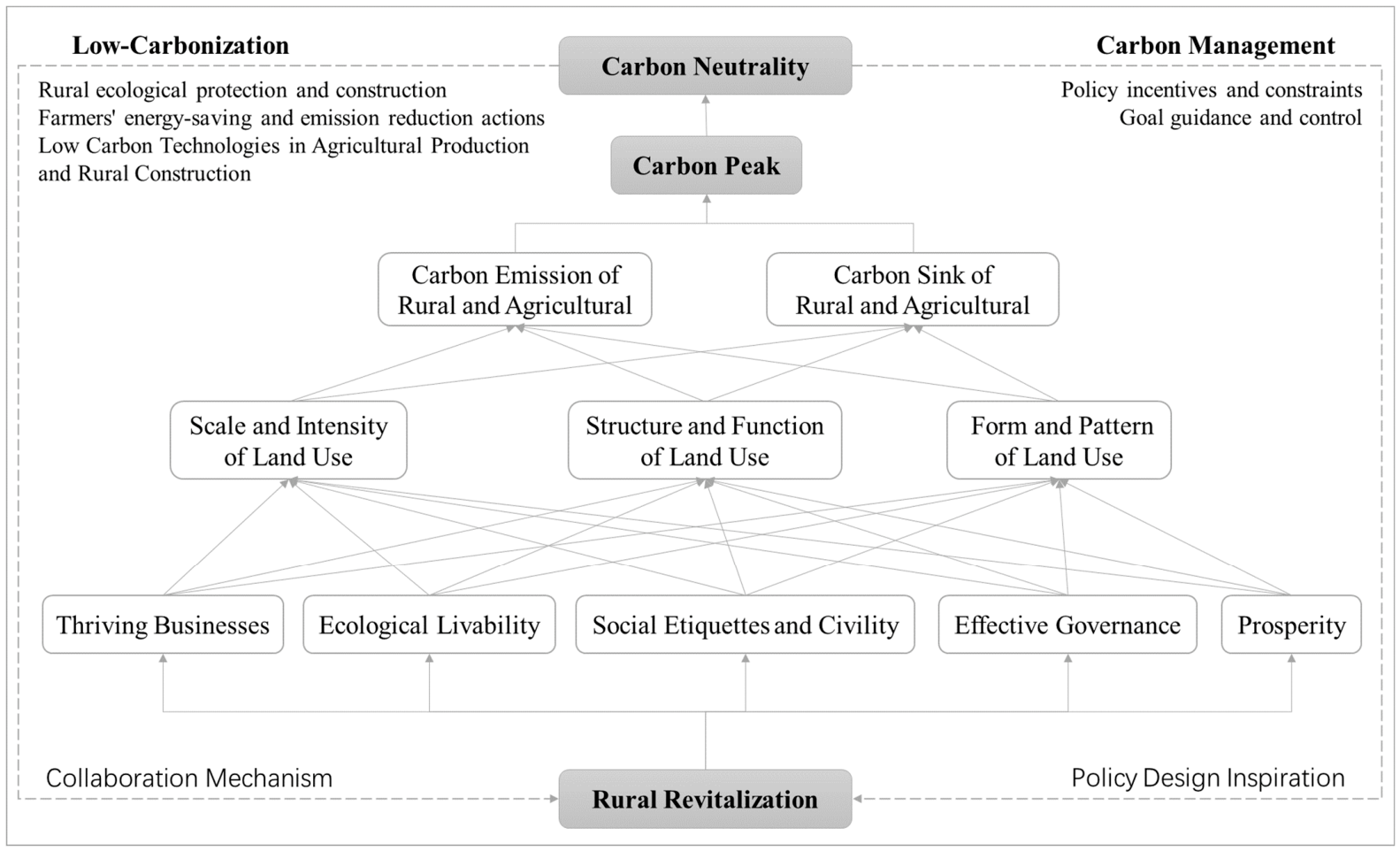
The Rural Revitalization Strategy is guided by the principles of “thriving businesses, pleasant living environments, social etiquette and civility, effective governance, and prosperity”. Under this guidance, significant changes have occurred in the scale, structure, form, and intensity of agricultural and rural land use in the western region. Through these dual pathways of “sources” and “sinks”, these changes have initiated a complex, nonlinear process of carbon-emission variation, which profoundly reshapes regional carbon-emission patterns and their decoupling effects (Figure 2). The thriving businesses drive the scaling and multifunctionalization of land use, fundamentally altering the balance between carbon sources and sinks in agricultural and rural land use. The pursuit of pleasant living environments drives the ecological and intensive use of land, exerting a two-way regulatory effect on carbon emissions. The construction of social etiquette and civility has facilitated the increase in public service and cultural land, exerting an indirect regulatory effect on carbon emissions. Effective governance drives land use standardization and institutional innovation, providing a mechanism to ensure the low-carbon transformation of land use. The shift in lifestyles and infrastructure upgrades driven by prosperity has had complex, two-way effects on carbon emissions from land use.
Changes in the scale, intensity, structure, type, form, and pattern of land use during rural revitalization exert dual impacts on carbon sources and sinks. The interplay between “emission-increasing” and “emission-reducing” forces across different regions directly leads to the diversification of agricultural and rural carbon emission evolution patterns. In western regions with varying resource endowments, rural revitalization may either result in a “lock-in effect” of carbon emissions or facilitate the attainment of an “inverted U-shaped” turning point. This multi-objective, multi-actor, and multi-pathway process of dynamic interplay and restructuring between “sources” and “sinks” means that carbon emission patterns do not follow a single linear trajectory, but instead exhibit regional heterogeneity characterized by both contraction and expansion [28]. The relationship between land use, carbon emissions, and rural revitalization is diverse, with decoupling, negative decoupling, and coupling coexisting. Due to disparities in resource endowments, development stages, and governance capacities, the level of rural revitalization in western China demonstrates significant spatial heterogeneity. These substantial differences also lead to variations in land-use transition patterns and their carbon effect directions. The implementation of the Rural Revitalization Strategy has profoundly transformed the patterns of “sources” and “sinks” of carbon emissions from land use by reshaping industries, ecosystems, and living spaces. Both rural revitalization and carbon emission evolution patterns are becoming increasingly complex, resulting in diverse decoupling relationships characterized by the coexistence of decoupling, negative decoupling, and coupling states [29].
Hypothesis 1.
The evolution patterns of land-use carbon emissions are diversified, and their decoupling relationship with rural revitalization varies.
In the context of rural revitalization, the decoupling of land-use carbon emissions is not a linear superposition of single elements but rather the product of nonlinear synergistic interactions among multidimensional factors such as population, industry, urbanization, industrialization, education, and culture [30]. The production of the decoupling effect is a complex process involving multifactorial, nonlinear interactions; empirical research must fully account for the combined effects of threshold, interaction, and spatial effects in order to accurately uncover its underlying influencing mechanisms [31]. The impact of each influencing factor on the decoupling relationship exhibits significant nonlinear characteristics, with distinct threshold and cutoff effects. The pathways of factor effects may exhibit various nonlinear forms, such as U-shaped, inverted U-shaped, S-shaped, or parabolic curves, featuring critical thresholds in the influencing mechanism with turning points like “increase-then-decrease”, “decrease-then-increase”, “positive-to-negative”, or “negative-to-positive” [32]. Interventions below the threshold may yield limited effects, whereas crossing the threshold can trigger a qualitative shift in the decoupling state. The influence of factors exhibits significant spatial effects, characterized by pronounced spatial heterogeneity and spatial correlation [33]. In western China, diverse geographical units such as mountainous areas, river valleys, and urban-rural fringes exhibit vast differences in resource endowments, economic development stages, and rural revitalization implementation pathways. This leads to stark variations in the direction and intensity of the same factor (e.g., industrial transformation) on decoupling across different spatial units, resulting in spatial heterogeneity. Meanwhile, carbon emissions from land use and the factors influencing rural revitalization inherently exhibit spatial mobility and spillover effects; land reclamation, industrial relocation, or ecological conservation in one region may have positive or negative spatial correlations and spillover effects on the carbon emission patterns of neighboring regions.
Hypothesis 2.
The decoupling effect results from the nonlinear synergistic interaction of multiple factors, with its influencing mechanisms exhibiting significant threshold and spatial effects.

2.3. Research Method

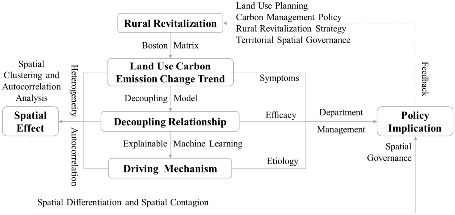
This study aims to systematically reveal the decoupling effect between rural revitalization and carbon emissions in western China and its influencing factors. To this end, it establishes a comprehensive analytical framework that combines “spatiotemporal pattern identification + value status diagnosis + influencing mechanism analysis” by integrating multiple econometric models, including Exploratory Spatial Data Analysis (ESDA), Boston Consulting Group Matrix (BCGM), decoupling model (DM), and explainable machine learning (EML). ESDA is used to uncover the spatial dependence between rural revitalization and carbon emissions. Through global and local spatial autocorrelation tests, it identifies spatial clustering patterns, providing a spatial foundation for subsequent analysis. Its advantage lies in quantifying spatial correlations, making it suitable for the macro context of regional disparities. BCGM integrates stock (relative share) and increment (growth rate) to precisely identify the spatiotemporal evolution trends of rural revitalization and carbon emissions in each region. DM dynamically quantifies the elastic relationship between rural revitalization and carbon emissions, transforming abstract sustainable development states into quantifiable, comparable policy signals and value orientations. EML accurately identifies the direction, intensity, path, and geographical differences in influencing factors. Its strength lies in fully adapting to the complex regional mechanisms of the western regions by overcoming the linear assumptions of traditional regression analysis. The methods are interlinked and mutually supportive. The analytical findings from the preceding methods provide data and conclusions that underpin subsequent research, thereby forming a closed-loop empirical analysis that enhances the scientific rigor and systematic approach of the study (Figure 3).

2.3.1. Spatial Clustering and Autocorrelation Analysis

This study assesses spatial heterogeneity for indicators through the coefficient of variation. The geographical distribution patterns of these factors are then visualized using quantile-based spatial clustering methods. Elevated coefficients of variation correspond to heightened spatial heterogeneity. To investigate spatial dependence, Moran’s I is introduced in this study to assess the spatial autocorrelation linking rural revitalization and carbon emissions. Additionally, the Getis-Ord Gi * method is applied to graphically display the spatial patterns of “hot spots” (high-value clusters) and “cold spots” (low-value clusters). This approach aids in revealing areas with typical spatial correlations between rural revitalization and carbon emissions [34]. Defined on a scale from −1 to 1, Moran’s I index exhibits a property whereby the intensity of observed spatial autocorrelation increases monotonically with its absolute value [35].

2.3.2. Boston Matrix

Originally from corporate strategic management, the Boston Consulting Group Matrix (market growth rate-relative market share matrix) simplifies complex strategic analysis. Its core appeal is an intuitive framework that classifies scenarios with clarity and ease. Although the matrix originated in the business world, its core logic can be creatively applied to this study. The relative share is the ratio of each city’s rural revitalization index to its carbon emissions, divided by the maximum value in the western region. The growth reflects the average annual increase in the rural revitalization index and carbon emissions from 2010 to 2020. The calculation formulas are shown in (1) and (2) [36]. Using the average values of relative share and growth rate as thresholds, the western region is divided into four categories: High Share-High Speed (Star), High Share-Low Speed (Cow), Low Share-High Speed (Gazelle), and Low Share-Low Speed (Dog).
R S = Z i Z i m a x × 100 %
G R = Z i e n d Z i b a s e t 1 × 100 %
where R S and G R represent relative share and growth rate, reflecting the stock and incremental characteristics of a region’s rural revitalization or carbon emissions in western China; Z i represents the rural revitalization index or carbon emissions scale of the ith region; Z i m a x represents their maximum value; Z i b a s e and Z i e n d represent the values at the baseline and end periods, respectively; n is the number of regions in the study area.

2.3.3. Decoupling Model

This study provides a systematic analysis of the dynamic decoupling relationship between the rural revitalization process and carbon emissions in western China using the Tapio decoupling model. The Tapio decoupling model was proposed by Finnish scholar Tapio in 2005, which is an improvement on the traditional OECD decoupling indicator. By calculating the elasticity ratio between the growth rate of carbon emissions and that of economic growth, it categorizes the relationship between the two into eight types using thresholds of 0.8 and 1.2: strong decoupling, weak decoupling, expansive coupling, expansive negative decoupling, recessive decoupling, recessive coupling, weak negative decoupling, and strong negative decoupling [37]. The 8 types can be further summarized into 3 categories, including decoupling, negative decoupling, and coupling. This model not only identifies decoupling states but also distinguishes the intensity, direction, and developmental stage of decoupling, demonstrating strong dynamic capabilities and explanatory power. With ε serving as the decoupling index, α as the average annual growth rate of carbon emissions, R A L U C E i and R A L U C E i + n as the total carbon emissions in the ith and i + n th years, respectively, β as the average annual growth rate of the rural revitalization index, R R I i and R R I i + n as the rural revitalization indexes in the ith and i + n th years, respectively, n as the study period, the formula for calculating the decoupling index between rural revitalization and carbon emissions is [38]:
ε = α β ,     α = R A L U C E i + n R A L U C E i n   1 ,       β = R R I i + n R R I i n     1

2.3.4. Explainable Machine Learning

This study analyzes the mechanism of action of each influencing factor on the decoupling relationship through the SHAP (SHapley Additive exPlanations) model of machine learning. The core advantage of this model lies in decomposing the prediction results into the contribution values of individual input features, enabling the interpretation of decision-making processes within the machine learning model and significantly enhancing the credibility of the mechanism explanation [39]. Let m be the serial number of machine learning samples, n be the total sample size, h be the specific feature of the m -th sample, Y b a s e represent the baseline value of the entire model, typically the mean of the target variable across all samples, and f X m h be the SHAP value of the hth feature for the mth sample, i.e., its contribution to the predicted value Y m , f X m h > 0 indicates that the feature has a positive effect on the prediction. Let C h ¯ be the mean of the absolute values of the global SHAP values for feature h, the explainable machine learning-related equation is [40]:
Y m = Y b a s e + f X m 1 + f X m 2 + + f X m h
C h ¯ = 1 n m = 1 n | f X m h |

2.4. Indicator Selection and Data Source

2.4.1. Land Use Carbon Emissions: LUCE

The land use carbon emissions data are sourced from the CHINA CITY CARBON DIOXIDE EMISSIONS DATASET released by the China Urban Greenhouse Gas Working Group. The China City Greenhouse Gas Working Group was initiated and organized by the Center for Climate Change and Environmental Policy Research of the Chinese Academy of Environmental Planning under the Ministry of Ecology and Environment. It has released comprehensive and full-coverage datasets for the years 2000, 2005, 2010, 2015, and 2020. The foundational data for this dataset comes from three sources: first, the China High Resolution Emission Gridded Data; second, official city-level data (including statistical yearbooks, government documents, and research reports); and third, data obtained through on-site surveys, interviews, telephone consultations, and official requests to departments involved by the working group. The dataset covers all cities and autonomous prefectures in China, encompassing direct and indirect carbon emission data across multiple sectors such as agricultural and industrial production, urban and rural living, roads, transportation, and energy [41]. The LUCE defined in this study constitutes a comprehensive aggregation of greenhouse gas emissions encompassing three core domains: agricultural production, rural livelihoods, and rural construction. In agricultural production, LUCE refers to greenhouse gas emissions generated throughout the entire agricultural production process due to material cycles, energy consumption, and production activities, primarily centered around the three key segments of “cropping, animal husbandry, and industrial chain support” [42]. LUCE in farmers’ lives refers to greenhouse gas emissions generated from daily production, living, and consumption activities, including energy use, waste disposal, and transportation, with a focus on the full spectrum of “clothing, food, housing, mobility, and utilities” scenarios [43]. Regarding rural development, LUCE refers to greenhouse gas emissions generated during infrastructure construction, public service facility operations, and village spatial improvements. These emissions result from building material consumption, energy usage, and construction activities, representing emissions that accompany rural development and spatial expansion [44].

2.4.2. Rural Revitalization Index: RRI

The rural revitalization index was calculated using the analytic hierarchy process and the entropy method, and an evaluation index system for the rural revitalization index was constructed, which includes 5 subsystems and 30 measurement indicators (Table 1). The selection of indicators is based on the following reasons. First, it must align with the national policy directives, including the Strategic Plan for Rural Revitalization (2018–2022) and Opinions on the Implementation of Rural Revitalization Strategy. Therefore, these five elements are selected as the first tier of the indicator system. Second, the calculated data referred to the research results of scholars such as Xu [45] and Yang [46]. Specifically, this study calculates the RRI in five steps based on their approach. Step 1: Standardize and normalize all indicators using the Max-Min method. To avoid meaningless zeros in entropy and logarithmic calculations, 0.01 is added uniformly to all indicators. Step 2: Calculate the proportion of each indicator across all regions. Step 3: Calculate the entropy value for each indicator. Step 4: Calculate the coefficient of variation and weight for each indicator. Step 5: Calculate the RRI for each region using a weighted sum. Their approach aligns with China’s policy orientation and the practical needs of rural revitalization, having gained widespread support and recognition from a large number of scholars [47]. Third, account must be taken of the realities of rural development strategies in Western China and the attainment of carbon peaking and carbon neutrality goals. For instance, consolidating and expanding the achievements of poverty alleviation while effectively advancing rural revitalization constitutes the foremost task for these areas. Therefore, both rural revitalization and the realization of carbon peak and carbon neutrality objectives must be grounded in the foundation of lifting people out of poverty. Data sources include statistical yearbooks, bulletins, and the Wind database from 11 provinces, autonomous regions, and municipalities. Wind, headquartered in Shanghai with 48 branches worldwide, is a leader in China’s information services industry. This study is primarily based on data from databases covering the economy, industries, enterprises, and satellite nighttime light.

2.4.3. Dependent and Independent Variable

The independent variables are the decoupling relationship between LUCE and RRI, with 11 indicators as independent variables. The selection of these substitute variables takes into account the multidimensional nature of rural revitalization, carbon peaking, and carbon neutrality, while also incorporating the regional particularities of the western regions. This methodology is supported by both theoretical and practical considerations. Table 2 shows that the VIF values for all factors are less than 10, indicating no significant collinearity among the factors. Notably, the VIFs for urbanization rate and average years of education are slightly above 5, suggesting mild collinearity. On the one hand, China has implemented a strategy for the coordinated development of urbanization and rural revitalization, and has long pursued education-driven development policies, making these two indicators indispensable to both rural revitalization and carbon emissions management. On the other hand, our empirical analysis employs the Explainable Machine Learning model, which is insensitive to collinearity while possessing unique advantages for handling high-dimensional data. Therefore, the final indicator system still retains the urbanization rate and average years of education. Data sources include the Seventh National Population Census of China, the Third National Land Survey, the China Urban Statistical Yearbook, along with regional yearbooks, bulletins, and government work reports.
The RP ( X 1 ), representing the demographic base engaged in production and daily life, constitutes the fundamental entity whose basic needs generate carbon emissions [48]. Its size dictates total agricultural inputs and baseline energy use. Through scale effects, population agglomeration can enhance resource allocation efficiency and lower per-unit emissions, with the rationality of such agglomeration directly affecting decoupling performance.
Against the backdrop of the comprehensive advancement of the rural revitalization strategy, disparities in land-use complexity exert a profound influence on the spatial layout of rural industries, the construction of living environments, and the conservation of ecological spaces, thereby impacting the quality of rural socio-economic development and changes in carbon emission intensity. This study employs LUCV ( X 2 ) to quantitatively measure land use complexity. The magnitude of entropy can intuitively reflect the equilibrium of land allocation and the systematic orderliness. A higher entropy value indicates a richer set of land-use types and more complex structures, whereas a lower value suggests a singular land-use structure and relatively concentrated spatial functions [49].
PAI ( X 3 ), reflecting structural shifts in the rural labor force, exerts a dual influence on decoupling [50]. In western rural China, the out-migration of younger adults has led to an aging rate above the national average. An elderly workforce often adheres to traditional, extensive farming methods characterized by high fertilizer/pesticide inputs and low efficiency, which may impede decoupling. Conversely, the frugal consumption patterns typical of older populations can lower household carbon emissions.
POMI ( X 4 ) is a hallmark of Western rural areas. Labor migration shrinks the agricultural labor pool and promotes land consolidation and scaled operations, thus improving productivity and reducing emissions. However, episodic surges in emissions can occur due to housing construction and consumption upgrades by returning migrants, rendering these dynamic fluctuations a critical variable in decoupling [51].
UR ( X 5 ) mirrors the flow of resources between rural and urban sectors. It reduces on-farm emissions through labor shift and fosters decarbonization via urban-driven technology and capital diffusion [52].
The level of industrialization is represented by PCGDP ( X 6 ). Industrial scale expansion increases carbon emissions, but economic growth also drives investment in low-carbon technologies and industrial upgrading, thereby curbing emissions growth [53].
The FSSR ( X 7 Farming Structure Synergy Ratio reflects the policy implementation capacity of local governments. Most Western regions depend on fiscal transfers. Higher self-sufficiency rates enable better implementation of low-carbon subsidies and promotion of energy-saving technologies, directly fostering decoupling. Conversely, low self-sufficiency may delay low-carbon policy execution due to funding constraints, becoming a limiting factor for decoupling [54].
ISRI ( X 8 ) reflects the efficiency of resource allocation and the level of coordinated development among rural industries; improving this index helps promote efficient integration between agriculture and non-agricultural industries and reduce the share of inefficient, resource-intensive industries [55]. It not only enhances rural revitalization through industrial upgrading and efficiency gains but also reduces the carbon emission intensity per unit of economic output, thereby strengthening the decoupling trend between economic growth and carbon emissions. This indicator is selected because it accurately captures the transition of rural industries from extensive expansion to intensive and efficient development, serving as a critical nexus connecting industrial revitalization with low-carbon development.
Excessive regional development inequality leads to resource misallocation, uneven provision of public services, and hindered diffusion of green technologies. It not only constrains the holistic advancement of rural revitalization but also tends to trigger high-carbon and extensive development in certain areas, thereby weakening the decoupling effect. Regional development disparities are a key challenge that must be addressed in the process of rural revitalization, and they are also a critical moderating factor influencing the decoupling of carbon emissions [56]. This study employs the Theil index, calculated using nighttime light data, to characterize regional development inequality, denoted as DII ( X 9 ).
AYE ( X 10 ) represents the level of rural human capital. Enhanced educational attainment helps strengthen farmers’ awareness of green production, increase the adoption rate of low-carbon technologies, and improve employment transition capabilities [57]. It provides support for the revitalization of rural talent while helping to achieve a win-win outcome of development and emissions reduction by slowing the growth of carbon emissions through the adoption of greener production methods. The selection of this indicator is due to the fact that human capital is a core element shared by rural revitalization and low-carbon transformation, and its differences directly determine the ability for green development and the path to decoupling.
PEMP ( X 11 ) reflects the characteristics of rural social structures; ethnic minority-concentrated areas often share features such as significant ecological importance, weak economic foundations, and traditional development models, and changes in their proportion can influence livelihood patterns, land use intensity, and the effectiveness of policy implementation [58]. This concerns the unique nature and precision of rural revitalization in ethnic minority regions, and also affects carbon emission patterns and the decoupling process. Calculating this indicator using the permanent resident population as the denominator provides a more accurate reflection of how the actual residential population structure affects rural development and carbon emissions, avoids statistical biases associated with the registered population, and enhances the practical relevance of the analysis.

3. Results

3.1. Spatiotemporal Evolution Characteristics of LUCE

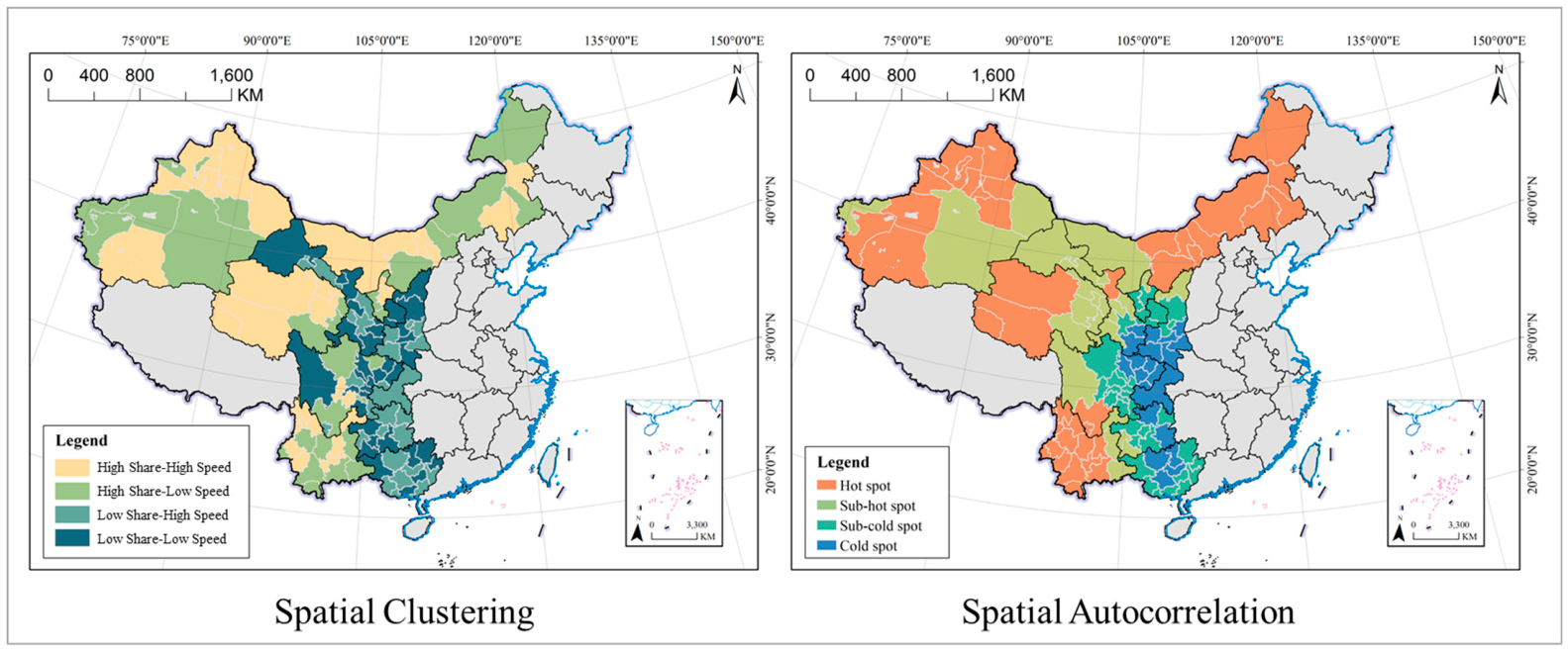
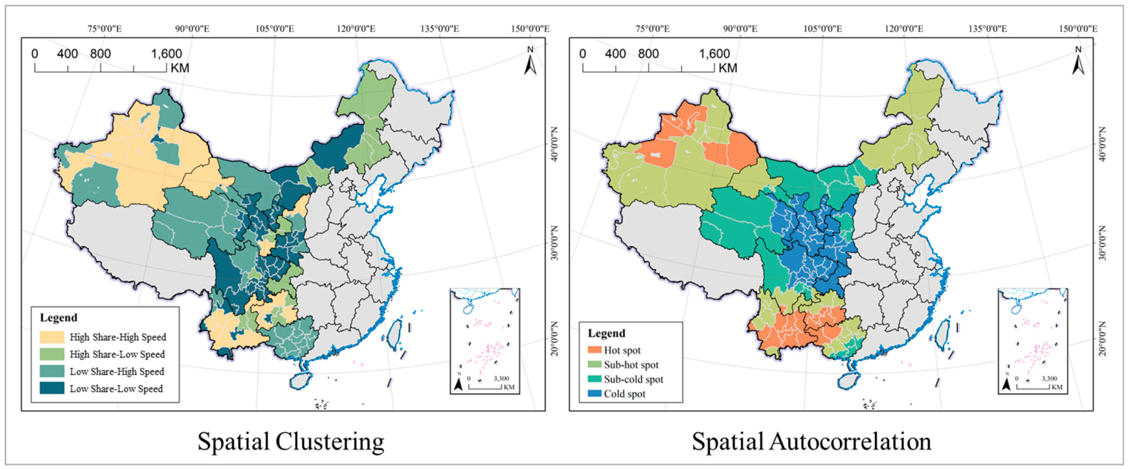
The average growth of LUCE in western China from 2010 to 2020 was 3.64%, with an average relative share of 0.20. Using them as thresholds, rural areas in the western region were classified into four categories based on carbon emissions levels. Moran’s I of the four categories of regions was 0.34 (Z = 6.56, p = 0.001), indicating a significant spatial positive autocorrelation in the spatiotemporal evolution of rural rejuvenation in China. Areas with high LUCE tend to cluster near similar areas, while low-emission regions also show spatial concentration. Hotspot areas are concentrated in border regions, including the Yunnan-Guangxi-Guizhou junction in the southwest and Xinjiang in the northwest. Coldspot areas cluster around the intersections of multiple provinces, such as Chongqing, Sichuan, Qinghai, Gansu, and Shaanxi, located in the inland hinterland (Figure 4).
There are 24 regions classified as high share-high speed, including Liupanshui, Zunyi, Bijie, Qianxinan, Qiandongnan, Baoshan, Zhaotong, Pu’er, Lincang, Chuxiong, Honghe, Wenshan, Dali, Yulin, Jiuquan, Longnan, Kumul, Changji, Bortala, Bayingolin, Aksu, Kashgar, Yili, and Tacheng. These regions face pressures of high existing emissions and rapid growth, with most located in the karst terrain of southwest China and the arid areas of northwest China. They represent key areas for future carbon emission reduction control. The “high share-low speed” category has the fewest members. These are mainly distributed in eastern Inner Mongolia (Baotou, Chifeng, etc.) and the Chengdu-Chongqing urban agglomeration and surrounding areas, composed of 16 regions: Baotou, Chifeng, Tongliao, Hulunbuir, Ulanqab, Hinggan, Chongqing, Chengdu, Guiyang, Tongren, Qiannan, Kunming, Qujing, Tianshui, Pingliang, and Qingyang. These areas have a large LUCE base, but growth has slowed and entered a plateau phase. There are 34 regions classified as low share-high speed, mainly located in Guangxi, Qinghai, and surrounding areas, including Alxa, Nanning, Liuzhou, Guilin, Wuzhou, Beihai, Fangchenggang, Qinzhou, Guigang, Yulin, Baise, Hezhou, Hechi, Laibin, Chongzuo, Ya’an, Aba, Nujiang, Diqing, Yan’an, Shangluo, Zhangye, Gannan, Haibei, and Hainan. These regions currently have low carbon emissions, but exhibit rapid growth, making them potential future hotspots. Most are late-developing areas undergoing critical phases of industrial transfer, large-scale infrastructure, and public service facility construction. The “low share-low speed” group is the largest. Most cluster in a belt-like pattern west of the Hu Line, including 50 regions like Alxa, Nanning, Liuzhou, Guilin, Wuzhou, Beihai, Fangchenggang, Qinzhou, Guigang, Yulin, Baise, Hezhou, Hechi, Laibin, Chongzuo, Ya’an, Aba, Nujiang, Diqing, Yan’an, Shangluo, Zhangye, Gannan, Haibei, and Hainan. Regions are already in an ideal low-carbon state—characterized by low emissions and slow growth.

3.2. Spatiotemporal Evolution Characteristics of RRI

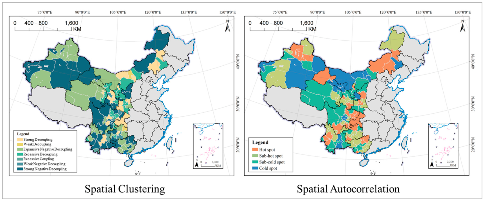
The average growth of RRI in the western region from 2010 to 2020 was 1.82%, with an average relative share of 0.30. Based on these thresholds, the western region was divided into four types of regions according to the rural revitalization level. The Moran’s I index for the four categories of regions was 0.48 (Z = 9.24, p = 0.001), indicating that the spatiotemporal evolution of China’s rural revitalization exhibits significant positive spatial autocorrelation. Hotspots are clustered in Yunnan, Xinjiang, Qinghai, and Inner Mongolia. Coldspots are mostly concentrated at the junction of Chongqing, Sichuan, Gansu, and Shaanxi (Figure 5).
Thirty-five regions, including Hohhot, Baotou, Wuhai, Chifeng, Bayannur, Hinggan, Alxa, Leshan, Ya’an, Kunming, Yuxi, Baoshan, Zhaotong, Lijiang, Lincang, Nujiang, Diqing, Xining, Haibei, Hainan, Yushu, Haixi, Yinchuan, Wuzhong, Urumqi, Kumul, Changji, Hotan, Yili, Tacheng, and Altay, fall under the high share-high speed category. These regions serve as the “pacesetters” for rural revitalization in western China. They possess dual advantages of high levels and rapid growth. A total of 28 regions, including Tongliao, Ordos, Hulunbuir, Ulanqab, Xilingol, Zigong, Guangyuan, Aba, Liangshan, Qujing, Pu’er, Chuxiong, Honghe, Wenshan, Xishuangbanna, Dali, Dehong, Haidong, Huangnan, Guoluo, Shizuishan, Guyuan, Zhongwei, Karamay, Turpan, Bortala, Bayingolin, Aksu, and Kashgar, fall into the high share-low speed category. These regions have a solid foundation for rural revitalization but show slowing growth as they have entered a mature phase. A total of 30 regions, including Nanning, Wuzhou, Beihai, Yulin, Hechi, Laibin, Chongzuo, Chongqing, Chengdu, Panzhihua, Luzhou, Guiyang, Liupanshui, Zunyi, Tongren, Qiandongnan, Tongchuan, Baoji, Weinan, Hanzhong, Shangluo, Jiayuguan, Baiyin, Zhangye, Dingxi, and Linxia, fall under the low share-high speed category. These regions have a weak foundation for rural revitalization but demonstrate strong growth potential and a catching-up momentum, positioning them as future “star” reserve zones. A total of 31 regions, including Liuzhou, Guilin, Qinzhou, Guigang, Baise, Hezhou, Deyang, Mianyang, Suining, Neijiang, Nanchong, Meishan, Yibin, Dazhou, Bazhong, Ziyang, Ganzi, Anshun, Bijie, Qianxinan, Qiannan, Xianyang, Yulin, Ankang, Lanzhou, Jinchang, Tianshui, Wuwei, Pingliang, Jiuquan, Qingyang, and Longnan, fall under the low share-low speed category. These regions are characterized by underdeveloped rural revitalization and sluggish growth momentum, confronting a dual challenge.

3.3. Decoupling Effect Between LUCE and RRI

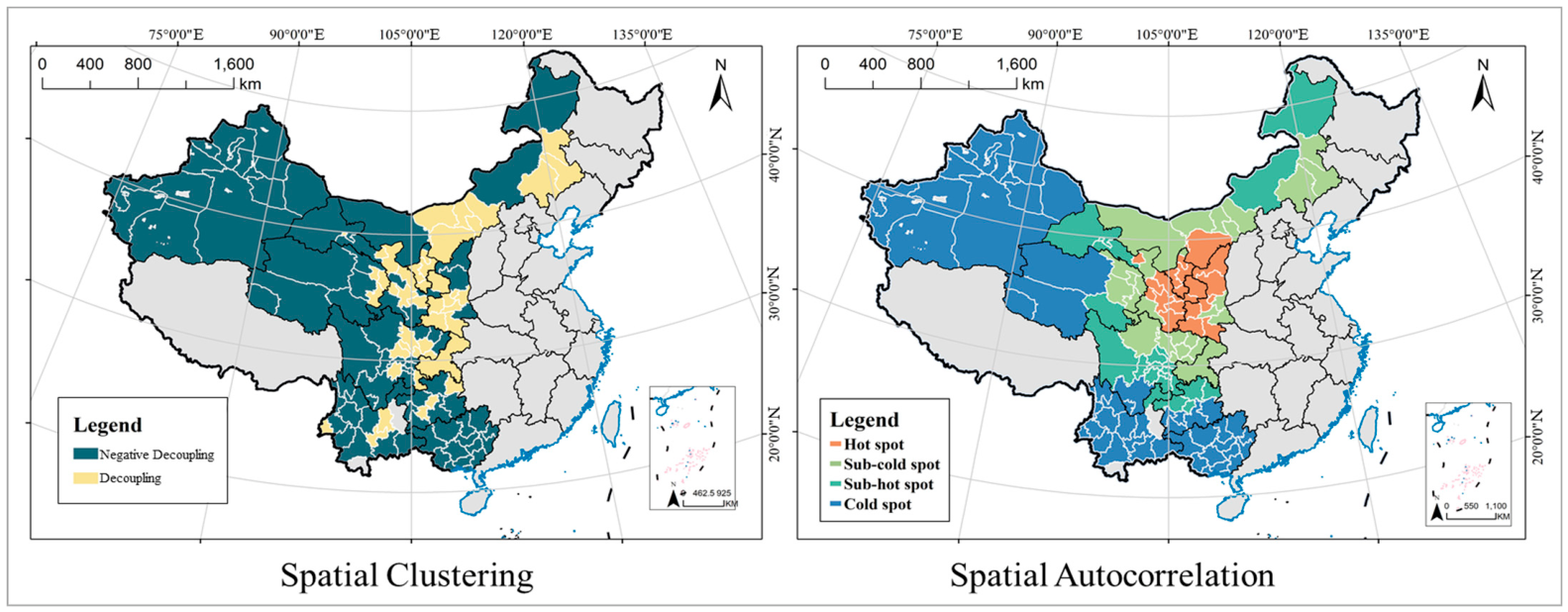
A clear pattern of differentiated decoupling emerges across the 124 western regions, where all but one (expansive coupling) of the eight theoretical types are present. In terms of frequency, strong decoupling (21 regions) and its negative counterpart (41 regions) dominate the landscape, constituting 50% of the total. This preponderance points to a pronounced polarization in the interplay between rural revitalization progress and carbon emission trajectories in the western region. Notably, the combined share of strong decoupling and expansionary decoupling exceeded 57%, highlighting that most regions in the West have yet to achieve high-quality low-carbon revitalization. It is evident that most regions in the West still face the dual predicament of “stagnant revitalization coupled with rigid emissions”. Moran’s I was 0.02 (Z = 1.64, p = 0.07), indicating a positive spatial autocorrelation in the decoupling relationship. However, the intensity was weaker than that of rural revitalization and LUCE. Hotspot areas were generally dispersed geographically, forming small clusters in the Chengdu-Chongqing metropolitan area, eastern Inner Mongolia, and northern Xinjiang. Most cold-spot areas were concentrated at the border between Gansu and Inner Mongolia (Figure 6).
A total of 21 regions are designated as strong decoupling areas, including Hohhot, Wuhai, Chifeng, Bayannur, Hinggan, Chongqing, Chengdu, Leshan, Guang’an, Guiyang, Kunming, Yuxi, Baoji, Weinan, Hanzhong, Jiayuguan, Baiyin, Dingxi, Linxia, Xining, and Yinchuan. The growth of rural revitalization in these regions is faster than that of carbon emissions, and the intensity of carbon emissions continues to decline. They have become a model for low-carbon rural revitalization in western China. Three regions exhibit weak decoupling, that is, Baotou, Tongren, and Tongchuan. They exhibit a slower growth rate in carbon emissions compared to rural revitalization, yet carbon emissions intensity continues to rise. Thirty-one regions fall under expansive negative decoupling, including Alxa, Nanning, Wuzhou, Beihai, Fangchenggang, Yulin, Hechi, Laibin, Chongzuo, Panzhihua, Ya’an, Liupanshui, Zunyi, Qiandongnan, Baoshan, Zhaotong, Lijiang, Nujiang, Diqing, Shangluo, and Zhangye. These regions experience rapid simultaneous growth in rural revitalization and carbon emissions, with carbon emissions intensity remaining persistently high, exhibiting a typical “high revitalization-high emissions” pattern. Twenty-two regions are classified as recessive decoupling, including Tongliao, Ordos, Ulanqab, Luzhou, Deyang, Mianyang, Suining, Nanchong, Anshun, Dehong, Xi’an, Xianyang, Ankang, Jinchang, Tianshui, Wuwei, Qingyang, and Haidong. They are characterized by simultaneous rural decline and reduced carbon emissions, yet carbon emissions intensity has not significantly improved. Qujing and Xishuangbanna exhibit a recessive coupling pattern, where rural decline coincides with a decrease in carbon emissions while maintaining high carbon-emission intensity. Four regions—Bazhong, Ziyang, Qiannan, and Lanzhou—demonstrate weak negative decoupling. They experience slower carbon emission reduction than rural decline, with carbon emission intensity slightly increasing. Forty-one regions exhibit strong negative decoupling, such as Hulunbuir, Xilingol, Liuzhou, Guilin, Qinzhou, Guigang, Baise, Hezhou, Zigong, Guangyuan, Neijiang, Meishan, Yibin, Dazhou, Aba, Ganzi, Liangshan, Bijie, Qianxinan, Pu’er, Lincang, Chuxiong, Honghe, Wenshan, Dali, Yan’an, Yulin, Pingliang, Jiuquan, Longnan, Gannan, Guoluo, Shizuishan, Karamay, and Turpan. In these regions, rural areas are declining while carbon emissions intensity continues to rise, creating a “high-carbon lock-in” effect and trapping them in a “low revitalization-high emissions” dilemma.

3.4. Nonlinear Mechanism of Decoupling Relationship

3.4.1. Model Construction and Parameter Analysis

Since the decoupling relationship is a non-numeric variable, a classification algorithm must be selected when performing modeling analysis using explainable machine learning. Due to the imbalance in sample size, there are very few regions in states such as recessive coupling and weak decoupling. Directly modeling with eight types would lead to distortion and failure of the constructed model. Therefore, the dependent variable is selected as decoupling categories instead of types, and Qujing and Xishuangbanna in the coupling state are excluded (Table 3). Among the dependent variables, there are 46 samples in a decoupling state, most of which are concentrated in the Loess Plateau, Inner Mongolia, and the Chengdu-Chongqing metropolitan area. There are 76 samples in negative decoupling, clustered in the northwest and southwest. Moran’s I is 0.29 (Z = 6.96, p = 0.000), indicating that the dependent variable exhibits significant positive spatial autocorrelation. The hotspots are located on the Loess Plateau, while the cold spots are situated in the northwest and southwest corners, forming a “center-periphery” spatial structure (Figure 7). The algorithms selected are CatBoost, LightGBM, and RandomForest, with a training and testing ratio of 60%: 40%. The robustness analysis is shown in Table 4. The training accuracy values are very close to 1, the testing accuracy values are all close to or exceed 0.7, and the degree of overfitting is less than 0.3, indicating that the machine learning models built using different algorithms are effective and highly robust. And based on the test recall and test F1 score, this study ultimately selects CatBoost’s output as the analysis results.

3.4.2. Nature and Intensity of Factor Influence

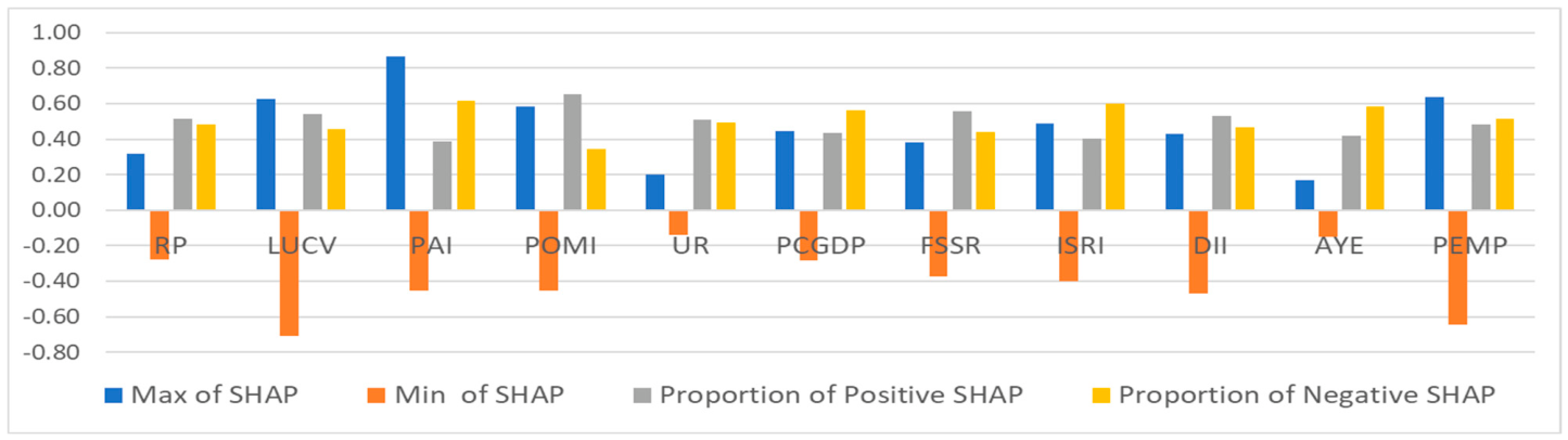
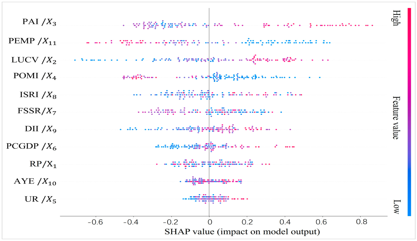
Figure 8 and Figure 9 illustrate the impact of the nature and intensity of each factor on the model output. The maximum SHAP values are all greater than zero, while the minimum values are all less than zero, indicating a mixed characteristic of factor influence. Judging by the ratio of positive to negative SHAP values, PAI ( X 3 ), PCGDP ( X 6 ), ISRI ( X 8 ), and AYE ( X 10 ) exhibit more prominent negative effects, while the positive effect of POMI ( X 4 ) is more prominent. The positive and negative effects of other factors are relatively balanced. PAI ( X 3 ), PEMP ( X 11 ), and LUCV ( X 2 ) rank as the top three in terms of influence, significantly higher than other factors. Their direct influence is already substantial, qualifying as a key factor. The western regions are home to a large number of ethnic minorities, whose unique patterns of production, daily life, and culture profoundly influence the local path to green development. In western rural areas with high proportions of ethnic minority populations, ecologically friendly traditional production and living practices are often preserved, such as reliance on organic fertilizers, minimal use of pesticides and fossil fuels, and inhabiting bamboo or wooden green buildings. Additionally, some ethnic minorities still uphold nature worship, which objectively safeguards the carbon sequestration functions of forests and grasslands, reducing ecosystem disturbances from ecotourism or specialized agricultural development. Therefore, the proportion of ethnic minority populations plays a significant moderating role in the decoupling relationship between rural revitalization and land use carbon emissions, enabling these regions to better achieve low-carbon development goals during the rural revitalization process. UR ( X 5 ) and AYE ( X 10 ) rank last in influence, significantly lower than other factors. They primarily rely on interaction effects to exert indirect influence, serving as auxiliary factors. The influence of other factors lies between key and auxiliary, with neither direct nor indirect effects negligible, classifying them as important factors.

3.4.3. Nonlinear Paths and Threshold Effects of Factor Influence

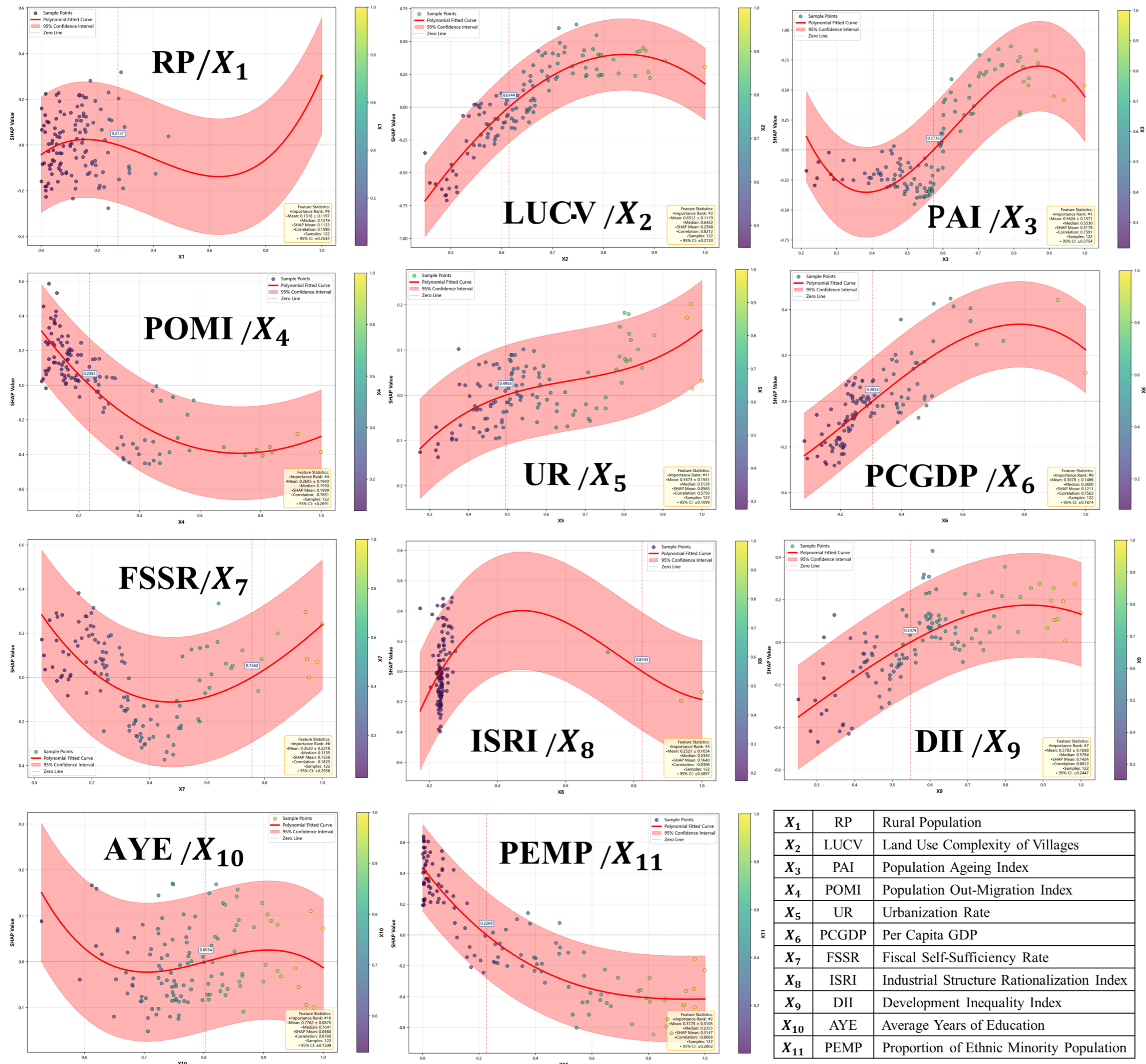
Figure 10 shows the influence pathways of each factor, all exhibiting significant nonlinear characteristics. The effects of these factors exhibit a significant threshold effect, with their inflection points statistically summarized in Table 5. RP ( X 1 ), PAI ( X 3 ), and AYE ( X 10 ) display a wave-like pattern, with multiple thresholds observed in SHAP values. LUCV ( X 2 ), PCGDP ( X 6 ), ISRI ( X 8 ), and DII ( X 9 ) exhibit an inverted U-shape, while POMI ( X 4 ) and FSSR ( X 7 ) display a U-shape. The SHAP value presents 2–3 thresholds, respectively representing the inflection points of the Impact Nature and Intensity mutations. UR ( X 5 ) shows an ascending arc, whereas PEMP ( X 11 ) exhibits a descending arc. There is only one threshold for the SHAP value, and the impact nature reverses before and after the threshold.
For instance, as population size increases from extremely low to extremely high, its impact on the decoupling relationship exhibits a nonlinear fluctuation pattern characterized by “negative → positive → peak → negative → trough”. In areas with minimal population size, such as remote villages in western regions or severely hollowed-out and declining villages, any rural revitalization investments (e.g., road construction, healthcare facilities, agricultural water infrastructure) require substantial consumption of building materials and energy. Since newly built infrastructure or public facilities can only serve a small population, the per capita carbon cost becomes extremely high, hindering the development of decoupling. When the population size surpasses the threshold value of 0.05, its impact on decoupling shifts from negative to positive, peaking at 0.12. Population agglomeration increases the sharing rate of infrastructure and public facilities, with economies of scale driving down per capita carbon costs. Meanwhile, alongside rural revitalization, the increasing adoption of new and clean energy sources, coupled with rising population density and the goal of ecological livability, has spurred the construction of green spaces and environmental protection facilities, thereby promoting low-carbon production and lifestyle models. However, as the population size surpasses the threshold of 0.27, continued population agglomeration begins to exert pressure on facility supply and to increase construction density, thereby accelerating the growth rate of emissions. Its positive effect on the decoupling relationship shifts back to negative, reaching a trough at 0.65.

3.4.4. Spatial Effects of Factor Influence

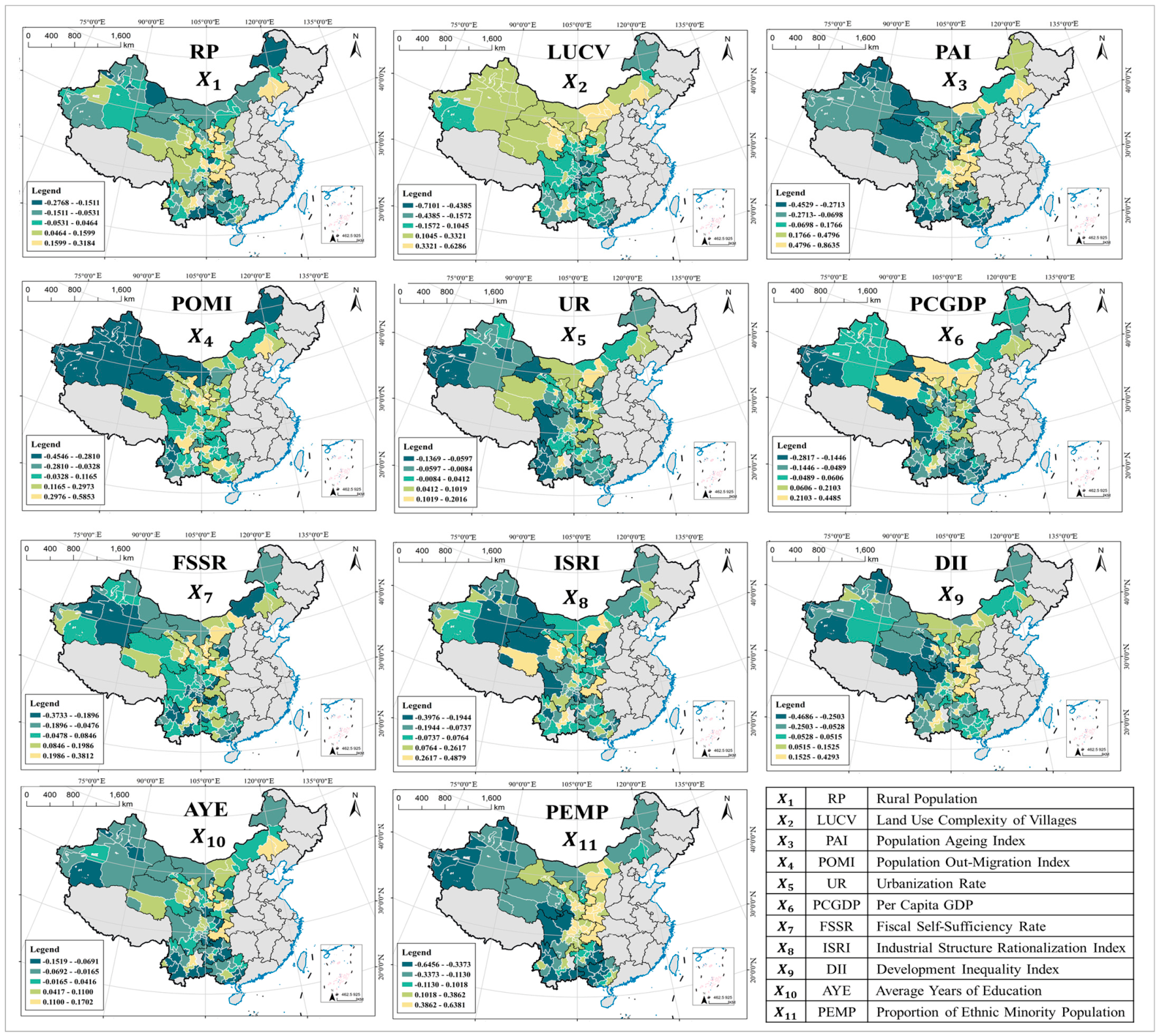
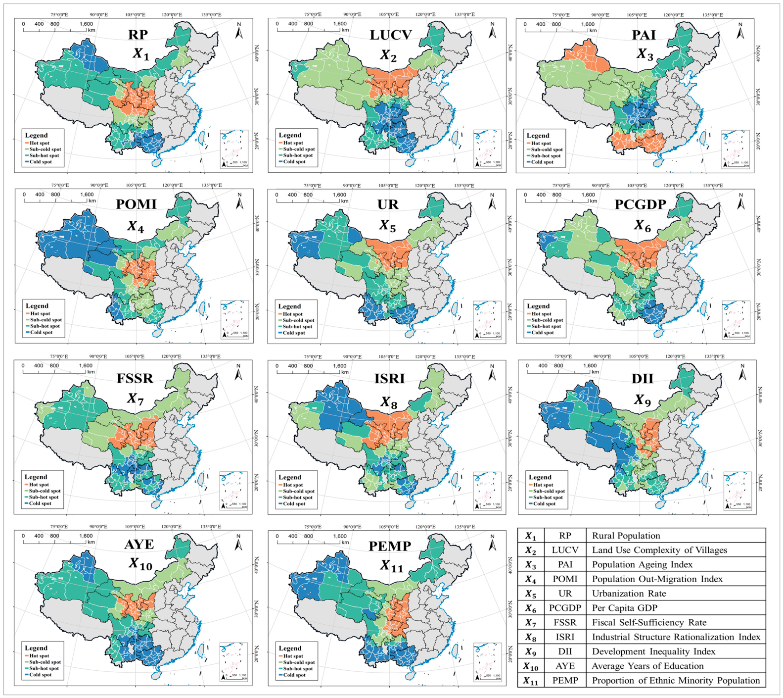
Table 6 displays the coefficient of variation and Moran’s I for the SHAP values of each factor, while Figure 11 and Figure 12 visualize the spatial heterogeneity and autocorrelation of the SHAP values, respectively. The absolute values of the coefficient of variation are all significantly greater than 0.36, indicating pronounced spatial heterogeneity in factor effects. FSSR ( X 7 ), ISRI ( X 8 ), DII ( X 9 ), AYE ( X 10 ), and RP ( X 1 ) exhibit far greater spatial heterogeneity than other factors. RP ( X 1 ) shows positive high-value clustering in the Loess Plateau and the Chengdu-Chongqing urban agglomeration, while negative high-value clustering occurs at the northern and southern extremities. LUCV ( X 2 ) exhibits high positive clustering in the northern regions, while high negative values are predominantly concentrated in the southwest. PAI ( X 3 ) and PEMP ( X 11 ) play a negative role in most regions, with their influence intensifying closer to the borders. Positive influences are largely clustered in the Shaanxi-Sichuan-Chongqing border region, with a few scattered in the Inner Mongolia Autonomous Region. POMI ( X 4 ) shows high negative clustering in the northwest, while positive and negative values coexist in other regions. UR ( X 5 ) displays high negative clustering in Xinjiang and Yunnan, while high positive values form a clustering belt in Chongqing, Shaanxi, Ningxia, and Inner Mongolia. The positive high values of PCGDP ( X 6 ) exhibit relative clustering in the northern regions, while the negative high values tend to aggregate toward the western and southern areas. The negative values of FSSR ( X 7 ) are relatively concentrated in Xinjiang, with high values forming a cluster centered around Ningxia. ISRI ( X 8 ) and DII ( X 9 ) display a mixed pattern of positive and negative values, with negative high values only relatively concentrated in Xinjiang. The negative high values of AYE ( X 10 ) are clustered in the Yunnan-Guizhou Plateau and Xinjiang in the northwest, while the positive high values are dispersed.
All Moran’s I values are positive and pass the significance test at the 0.03 level, indicating significant spatial autocorrelation in factor effects. LUCV ( X 2 ), PAI ( X 3 ), POMI ( X 4 ), and PEMP ( X 11 ) exhibit much higher spatial autocorrelation than other factors. RP ( X 1 ), POMI ( X 4 ), FSSR ( X 7 ), and AYE ( X 10 ) show highly similar hotspot distribution patterns, all clustered in the central Loess Plateau. LUCV ( X 2 ), UR ( X 5 ), PCGDP ( X 6 ), ISRI ( X 8 ) share nearly identical hotspot distribution patterns, concentrated in the border region of Gansu-Inner Mongolia-Ningxia-Shaanxi in the north. The hotspots of PAI ( X 3 ) form two clusters in Guangxi-Yunnan and Xinjiang, both adjacent to the border. The hotspot clusters of DII ( X 9 ) and PEMP ( X 11 ) are located in the central eastern region, covering Shaanxi and Ningxia, as well as adjacent areas of Sichuan and Gansu provinces. RP ( X 1 ), UR ( X 5 ), PCGDP ( X 6 ), AYE ( X 10 ), and PEMP ( X 11 ) each form a cold spot cluster in the north and south, located in Xinjiang in the northwest, and Yunnan and Guangxi in the southwest, respectively. Although the coverage varies slightly, the development of the northern and southern clusters is relatively balanced. Unlike them, the cold-spot clusters of POMI ( X 4 ) and ISRI ( X 8 ) exhibit uneven development, with the southern cluster being less mature. The cold spots of LUCV ( X 2 ) and FSSR ( X 7 ) are both concentrated in Chongqing, Sichuan, Guizhou, and Guangxi, but the former is well-developed, while the latter is immature. The cold spots of PAI ( X 3 ) are concentrated in the Chengdu-Chongqing urban agglomeration, located in the central region. The cold spots of DII ( X 9 ) are clustered on the western side, distributed across Xinjiang, Sichuan, and Qinghai.

4. Discussion

4.1. Situation Differentiation

Rural revitalization encompasses a systemic transformation across multiple dimensions, including industry, ecology, culture, talent, and organization, profoundly driving the restructuring of land-use and carbon-emission patterns. This results in significant spatial heterogeneity and hierarchical differentiation in their evolutionary trends. The thriving businesses drive the scaling and multifunctionalization of land use, fundamentally altering the balance between carbon sources and sinks in agricultural and rural land use [59]. Rural revitalization has driven the scaling, mechanization, electrification, and chemicalization of agricultural production methods. Changes in the intensity of rural and agricultural land use and input structures have triggered carbon-emission variations through energy consumption and material inputs. With the construction of high-standard farmland and large-scale operations, the widespread adoption of large agricultural machinery has substantially increased fossil energy consumption. While the intensive use of modern inputs such as chemical fertilizers, pesticides, and agricultural films has increased yields per unit area, it has also led to a rise in the carbon footprint of agricultural products per unit. The pursuit of pleasant living environments drives the ecological and intensive use of land, exerting a two-way regulatory effect on carbon emissions. The rural living environment improvement initiative has promoted the revitalization of “hollow villages” and the reclamation of idle residential land, optimizing village layouts, reducing the fragmentation of rural construction land, and generating substantial short-term embodied carbon emissions [60]. Reclaimed land is converted into farmland or ecological land through the policy of linking the increase and decrease in urban and rural construction land, thereby enhancing vegetation recovery and soil carbon sequestration capacity, which significantly boosts regional carbon sink functions in the long term. In ecologically sensitive areas, the program to convert farmland into forests and grasslands has been continuously expanded, transforming marginal farmland into ecological land. Land use has shifted from intensive agricultural production to ecological conservation, and carbon sink lands—such as forests, grasslands, and water bodies—have been protected and restored, directly enhancing the region’s carbon sequestration capacity. In addition, efforts to improve the appearance of villages have led to a steady increase in the scale of ecological land—including ecological corridors, small wetlands, and rural green spaces—thereby clarifying the boundaries between productive, residential, and ecological spaces within villages. This has directly reshaped the ecological foundation and living environment of the national territory, laying the ecological groundwork for the long-term decoupling of land use from carbon emissions [61].
This study conducted an in-depth analysis of the spatiotemporal characteristics of rural revitalization and carbon emissions in western China using the Boston Matrix and identified four types of dynamic evolution paths. High-share high-speed areas serve as “pacesetters” for rural revitalization but require prioritized carbon-emission control. High-share low-speed regions are the “mature zones” of rural revitalization and the “plateau zones” of LUCE. Low-share high-speed regions are the “rising zones” of rural revitalization and the “warning zones” of LUCE. Low-share low-speed regions are the “challenged zones” of rural revitalization and the “pioneers” in achieving rural carbon peak and neutrality goals. The decoupling relationship between rural revitalization and carbon emissions in western China shows polarized and diversified patterns. Strong decoupling and strong negative decoupling together account for 50%, reflecting the coexistence of “low-carbon revitalization models” and “high-carbon lock-in dilemmas”. Expansive negative decoupling and weak negative decoupling exceed 28%, highlighting that most regions have yet to achieve high-quality low-carbon revitalization. Spatial positive autocorrelation of decoupling is weak, but long-term clustering of hot/cold spots suggests regional embeddedness of decoupling patterns. To date, there is no sufficient research specifically analyzing the relationship between rural revitalization and the decoupling of carbon emissions from land use. A comparative analysis of similar studies reveals the unique value of our research. Xiao [62] believes that the relationship between cropland use, carbon emissions, and agricultural economic growth is predominantly characterized by strong decoupling, whereas Wang [63] suggests that the relationship between land use, carbon emissions, and economic growth is mostly weakly decoupled, which significantly differs from the findings of this study. The discrepancy arises because the former overlooked village land-use carbon emissions, and the latter failed to distinguish between urban and rural land-use carbon emissions. In addition, studies by other scholars have focused solely on the decoupling relationship between carbon emissions and economic growth, ignoring the non-economic dimensions of rural revitalization.
Previous studies often focused solely on the level of RRI or the scale of LUCE, emphasizing linear progress or regression in a single dimension [64,65]. In contrast, this study uses the Boston Matrix’s two-dimensional perspective (market share and growth rate) to more precisely characterize rural revitalization and carbon emissions profiles across regions. By uncovering the nonlinear and intricate evolutionary dynamics, this analysis helps bridge existing research gaps concerning the governance of rural revitalization and carbon emissions. The observed diversity in spatiotemporal evolution patterns poses a fundamental challenge to conventional governance frameworks, which tend to concentrate exclusively on either growth-oriented or stock-based dimensions. It inspires policy design to establish a comprehensive technical framework integrating both stock and growth [66,67]. A single emissions reduction pathway is unlikely to meet the complex and ever-changing demands of reality. To achieve the goals of “carbon peaking and carbon neutrality,” it is essential to design differentiated development pathways tailored to local conditions, based on the evolution of carbon emissions and their decoupling from rural revitalization. According to the theoretical framework, the rural revitalization strategy does not linearly influence agricultural and rural land use and their carbon emissions in isolation. Instead, it operates through multiple pathways, leading to diversified carbon emission evolution patterns and regional variations in decoupling relationships. This complexity makes it difficult for a single emissions reduction pathway to meet real-world needs [68]. To achieve the goals of “carbon peaking and carbon neutrality”, it is necessary to analyze trends in carbon emissions, take into account regional decoupling relationships, and design tailored pathways based on local conditions, thereby shifting the relationship between land use carbon emissions and rural revitalization from “passive conflict” to “active synergy”.
The polarization of decoupling relationships indicates that integrating the “dual carbon” goals with rural revitalization is not a simple matter of “addition” or “constraint”, but rather an issue of “quality” and “path”. Strong decoupling is itself the core essence and inherent requirement of high-quality rural revitalization. Regions in a state of “strong decoupling” serve as “showrooms” for the synergistic advancement of the “dual carbon” goals and the rural revitalization strategy. In contrast, the vast negative decoupling regions reveal deep-seated contradictions in current rural development models—either extensive growth leading to high environmental costs or stagnant development with inflexible carbon emissions [69]. This finding sounds an alarm: both “revitalization” efforts that disregard low-carbon boundaries and “carbon reduction” measures secured through developmental sacrifice are antithetical to sustainable development. Such an insight underscores the imperative to seamlessly weave the “dual carbon” goals into the very fabric of rural revitalization strategies [70,71]. The implication is that the “dual carbon” objectives ought to be integrated as intrinsic “foundational conditions” and “central metrics”—not relegated to external or subordinate “environmental goals”—within the entire cycle of rural revitalization, from planning and implementation to evaluation. To overcome specific decoupling bottlenecks, policy architecture should be precisely tailored: “benchmark-setting” for strong decoupling zones, “deadlock-breaking” for negative decoupling zones, and “increment-controlling” for transitional zones. This pathway is designed to drive a comprehensive regime shift in decoupling typologies from a state of “negative dominance” to one of “positive transformation,” guaranteeing that rural revitalization advances in synergy with national carbon peaking and carbon neutrality commitments.

4.2. Complex Mechanism

Explainable machine learning analysis reveals that the 11 factors shape decoupling through five attributes: mixed nature, hierarchical intensity, nonlinear pathways, spatial heterogeneity and autocorrelation, as well as interactive complexity. These attributes and characteristics yield specific leverage points for policy crafting. To understand the operative mechanisms, policymakers must develop a “force field diagram of influencing factors”. This diagram, by highlighting the chief limiting factors and primary enablers that vary by region, directly informs the design of customized intervention packages under a strict “one-region-one-policy” doctrine [72]. Most existing studies employ linear models and clearly distinguish between positive and negative factors. For instance, Du [73] posited that economic factors inhibit the decoupling of land-use carbon emissions, while population density and energy structure promote it. In contrast, this study adopts an interpretable machine learning model, revealing that all factors exhibit mixed characteristics.
This study classifies the influence of factors into three levels: key, important, and auxiliary. This approach is largely consistent with the views of other scholars, though differences lie in the criteria used to determine which level each factor falls into. For example, Liu [74,75] found that economic development, industrial structure, population size, and government intervention are key factors driving changes in land use carbon emissions, whereas this study finds that it relies more on interaction effects to exert indirect and auxiliary roles. Compared to the urbanization rate, PAI ( X 3 ), PEMP ( X 11 ), and LUCV ( X 2 ) are the most critical factors in the nonlinear model. Similarly, numerous scholars, including Zhang [17], Yang [46], Chen [76], and Li [77], have found that industrial structure and population size play a key role. This study supports and validates their perspectives while also revealing that the importance of these factors has been overestimated. Their research relies on a linear model that assumes additivity and the absence of interactions among variables, failing to identify nonlinear and threshold effects. This methodological limitation may lead to misidentifying significant factors as key drivers, potentially overestimating their influence. In contrast, our study utilizes a machine learning model that, through regularization, feature interaction, and ensemble learning, reduces the independent contribution of individual factors and allocates more explanatory power to interaction terms and nonlinear mechanisms. Additionally, machine learning offers greater predictive accuracy and generalizability, and its results better reflect the actual mechanisms underlying the decoupling of carbon emissions from land use in rural revitalization, thereby providing greater practical value.
This research uncovers the complex nonlinear mechanisms behind the decoupling of land-use carbon emissions during rural revitalization, which holds significant theoretical value and practical implications, representing the foremost academic contribution of this study. At the theoretical level, this study challenges traditional linear attribution assumptions. Employing interpretable machine learning models, it identifies multiple threshold effects and morphological heterogeneity (such as wave-shaped, inverted U-shaped, and U-shaped patterns) within the causal pathways of various factors. The study validates the theoretical hypothesis of multifactorial, nonlinear, synergistic drivers and deepens scientific understanding of the mechanisms underlying abrupt shifts in the decoupling of land use and carbon emissions [78]. At the practical level, it identifies critical thresholds and inflection points, providing a scientific benchmark for differentiated policy formulation [32]. By analyzing the “threshold changes” and “inflection points” of various factors, policymakers can accurately identify the “optimal window of opportunity” for intervention, thereby avoiding policy lags or excessive intervention.

4.3. Spatial Collaboration

Significant spatial heterogeneity and autocorrelation characterize the patterns of RRI, RALUCELUCE, the decoupling relationship, and the influence of all factors. This points to a fundamental reality: the western region constitutes a complex system of multiple “spatial clubs,” not a monolithic bloc. Geographically adjacent regions frequently share similar attributes, and this emergent “club convergence” is gaining strength over time, indicative of an intensifying Matthew effect [79]. The recognition of spatial clubs calls for a fundamental reorientation of policy design, prioritizing “spatial policies” over conventional “industry policies”. The latter often resort to undifferentiated tools—standard agricultural subsidies or uniform environmental rules—that overlook substantial regional variations. Such generic approaches are ill-suited to meet place-specific demands. Therefore, forward-looking governance must be spatially anchored: it requires the identification of discrete “spatial clubs” and the development of holistic, club-specific policy portfolios. Operationally, this transforms the core question of policy from “what industries to control” to “what mix of policies to deploy in what spatial units”. This evolution—from a “vertically fragmented” mode to a “horizontally integrated” one—is key to governance modernization and targeted zone management. Moreover, genuine spatial policymaking must rise above administrative silos, advancing from “fragmentation” to “systematization,” and from “compartmentalized actions within boundaries” to “joint governance by regional clubs” [80,81]. Effective policy design should foster cross-regional collaboration by creating shared resource pools, facilitating knowledge and technology transfer, and co-formulating regional green development strategies. Furthermore, accounting for spatial autocorrelation demands a dual approach that carefully balances “holistic coordination” against the need for “localized precision”. This necessitates implementing regionally differentiated measures that are custom-fit to address the specific constellations of challenges and opportunities present in each area.

5. Conclusions

Concurrently advancing the “dual carbon” goals and the rural revitalization strategy presents China’s western regions with the twin challenges of pursuing growth while mitigating emissions. This research, centered on these regions, establishes a comprehensive rural revitalization assessment framework comprising five key dimensions: economic, social, cultural, ecological, and political. Employing an integrated methodological toolkit—including the Boston Matrix, Tapio decoupling model, and explainable machine learning—the study investigates the spatiotemporal patterns, decoupling dynamics, and key drivers in the interplay between rural revitalization and carbon emissions from 2010 to 2020. This study verifies the theoretical hypotheses, and the principal findings of this investigation are summarized below:
First, both rural revitalization and land-use carbon emissions in western China follow discernibly dynamic evolutionary paths and display substantial spatial effects. The Boston Matrix further elucidates their divergent developmental trajectories. The state of rural revitalization is differentiated into four zone archetypes: leading, mature, rising, and challenged. Parallel analysis classifies LUCE into four regional profiles: critical, plateau, warning, and pioneering. Each archetype or profile is linked to a specific geographical footprint and entails a unique set of developmental challenges. The evolution of rural revitalization and land-use carbon emissions has significant positive spatial autocorrelation, with Moran’s I values of 0.34 (Z = 6.56, p = 0.001) and 0.48 (Z = 9.24, p = 0.001), respectively.
Second, a pronounced polarization characterizes the decoupling relationship between rural revitalization and LUCE, presenting a major obstacle to their coordinated advancement. Analysis reveals a spectrum of decoupling states across western China, yet two extremes—strong positive and strong negative decoupling—jointly account for half (50%) of all cases. Moreover, more than 57% of regions are locked in either expansive or strong negative decoupling, a clear signal that the majority have yet to realize high-quality low-carbon revitalization. These regions are frequently caught in a dualistic trap, typified either by “stagnant revitalization alongside rigid emissions” or by “low revitalization with high emissions”. This stark polarization delivers a critical warning: the integration of the dual carbon goals with rural revitalization transcends the mere imposition of constraints; at its heart, it is a foundational question of development quality and future pathway. Consequently, attaining strong positive decoupling constitutes the very core of what defines high-quality rural revitalization.
Third, the influencing factors exhibit mixed effects, varying intensity levels, nonlinear pathways, spatial heterogeneity, and autocorrelation in their impact on decoupling relationships. All factors demonstrate both positive promotion and negative inhibition effects. Based on their influence magnitude, they are categorized into three levels: key, important, and auxiliary. The population aging index, the proportion of the ethnic minority population, and the land-use complexity of villages are identified as key factors. The pathways of factor effects exhibit significant nonlinear characteristics, manifesting as wave-like, inverted U-shaped, and U-shaped patterns. The nature and intensity of factor effects undergo dynamic shifts, including “threshold mutations” and “inflection point reversals”, across developmental stages. The effects of these factors exhibit significant spatial patterns, with the fiscal self-sufficiency rate, industrial structure rationalization index, development inequality index, average years of education, and rural population showing more pronounced spatial differentiation. In contrast, the Land Use Complexity of Villages, Population Aging Index, Population Out-migration Index, and Proportion of Ethnic Minority Population exhibit stronger spatial correlations.
Fourth, the study yields a set of systematic, actionable policy implications. First and foremost, a fundamental shift in the governance paradigm is essential: a move away from traditional models centered on “industry policy” toward frameworks led by “spatial policy,” thereby enabling precise and differentiated governance grounded in zoning and functional classification. Concurrently, the “dual carbon” goals must be reconceptualized and deeply embedded as fundamental “prerequisites” and “core evaluation metrics” within the entire process of rural revitalization. Building upon this foundation, tailored strategies must be devised and implemented according to specific decoupling types, a targeted approach that is crucial for propelling a systemic transition from prevailing “negative-dominated” to desirable “positive-transition” decoupling trajectories. To support this transition, operational tools are required. This entails developing a dynamic, spatially explicit “map of influencing factor dynamics” to visualize evolving conditions. Based on such diagnostic maps, customized “one-place-one-policy” intervention plans can be formulated to directly address the dominant contradictions identified in each locale. Ultimately, transcending the constraints of administrative boundaries is imperative. The establishment of a “regional club collaborative governance” mechanism is vital to catalyze the overarching transformation of rural revitalization and carbon emissions governance—from a fragmented system based on “administrative districts” toward an integrated, synergistic “spatial network”.
Despite the achievements made in this paper, there are still limitations. First, the selection of influencing factors is primarily based on macro-level statistical data, failing to incorporate micro-level behavioral mechanisms, such as farmers’ low-carbon behavioral choices and the governance effectiveness of grassroots organizations. Second, the exploration of the underlying mechanisms behind the decoupling relationship between rural revitalization and carbon emissions remains insufficient, particularly regarding the role of soft factors such as institutional and cultural elements, as well as ecological factors such as ecological technologies and carbon sink capacity. Notably, while this study, based on historical data and machine learning models, reveals key influencing factors and nonlinear mechanisms of the decoupling relationship between rural revitalization and land-use carbon emissions, it remains challenging to prospectively predict long-term future evolution trends. Therefore, in future research, it can be considered to introduce computer simulation models, such as System Dynamics or Agent-Based Modeling, to conduct dynamic evaluation and scenario deduction of key indicators. Thus, the “retrospective” mechanism analysis is expanded to “prospective” prediction and decision support.

Author Contributions

Conceptualization, F.W.; methodology, F.W.; software, S.Z. and H.G.; validation, F.W. and S.Z.; formal analysis, Z.W. and S.Z.; investigation, F.W. and Z.W.; resources, F.W.; data curation, F.W. and Z.W.; writing—original draft preparation, F.W. and Z.W.; writing—review and editing, H.G. and S.Z.; visualization, S.Z.; supervision, F.W. and H.G.; project administration, Z.W. and H.G.; funding acquisition, F.W. and Z.W. All authors have read and agreed to the published version of the manuscript.

Funding

This research was funded by the National Natural Science Foundation of China (42401352) and the Natural Science Foundation of Guangdong Province, China (2025A1515010209).

Institutional Review Board Statement

Not applicable.

Informed Consent Statement

Not applicable.

Data Availability Statement

The data is sourced from China City Greenhouse Gas Working Group, link: https://www.cityghg.com/toCauses?id=4 (accessed on 1 March 2026).

Conflicts of Interest

The authors declare no conflicts of interest.

References

  1. Hu, J.H.; Song, M.F.; Zhang, L.W. Spatial and Temporal Evolution of Land Use Carbon Emission and Carbon Balance Zoning: Evidence from Xinjiang China. Sci. Rep. 2025, 15, 35705. [Google Scholar] [CrossRef] [PubMed]
  2. Li, X.P.; Hu, S.; Jiang, L.F.; Han, B.; Li, J.; Wei, X. Bibliometric Analysis of the Research (2000–2020) on Land-Use Carbon Emis-sions Based on CiteSpace. Land 2023, 12, 165. [Google Scholar] [CrossRef]
  3. Zhang, H.; Li, Y.B.; Xu, Q.; Yu, M.; Huang, J. Land Use Transition of the Mountain-Basin System Under the Background of Ru-ral Revitalization: Based on Four Typical Mountain-Basin Systems. Pol. J. Environ. Stud. 2022, 31, 3429–3445. [Google Scholar] [CrossRef]
  4. Yao, Y.; Lu, L.L.; Fu, Z.T.; Chen, F.; Wang, R.; Li, Q.T. Land Use Carbon Emission Projections in Shared Socioeconomic and Rep-resentative Concentration Pathways: Relationship with Urbanization in Chinese Megacities. Land Use Policy 2025, 157, 107659. [Google Scholar] [CrossRef]
  5. Zamora, C.; Masolele, R.; Berger, K.; Reiche, J.; Martius, C.; Verchot, L.; Szantoi, Z.; Herold, M. Refining Land-Use-Specific Carbon Emission Factors for Commodity-Driven Deforestation Monitoring in Colombia. Environ. Res. Lett. 2026, 21, 034018. [Google Scholar] [CrossRef]
  6. Le, H.T.D.; Nguyen, H.T.T. Remote Sensing and GIS Approaches to Carbon Emission Measurement as Related to Land Use Change in Phu Giao, Binh Duong Province, Vietnam. Eurasian Soil Sci. 2026, 59, 27. [Google Scholar] [CrossRef]
  7. Qiu, A.Y.; Yue, H.; You, Z.; An, H. Forecasting of Factors Influencing Carbon Emission from Land-Use in Liaoning Province, China, Under the “Double Carbon” Target. Ecol. Model. 2025, 509, 111255. [Google Scholar] [CrossRef]
  8. Xu, Q.Y.; Li, K.Q. Land Use Carbon Emission Estimation and Simulation of Carbon-Neutral Scenarios Based on System Dy-namics in Coastal City: A Case Study of Nantong, China. Land 2024, 13, 1083. [Google Scholar] [CrossRef]
  9. Zhuang, H.M.; Chen, G.Z.; Yan, Y.C.; Li, B.J.; Zeng, L.; Ou, J.P.; Liu, K.Y.; Liu, X.P. Simulation of urban land expansion in China at 30 m resolution Through 2050 Under shared socioeconomic pathways. GIScience Remote Sens. 2022, 59, 1301–1320. [Google Scholar] [CrossRef]
  10. Wang, Y.H.; Wang, H.W.; Sun, J.H.; Zhou, C.X.; Lin, X.F.; Liu, S.H.; Wang, C.P. Carbon Emission Patterns and Carbon Balance Zoning of Land Use in Xiamen City Based on Urban Functional Zoning. Land 2025, 14, 2197. [Google Scholar] [CrossRef]
  11. Li, R.; Zhang, J.S.; Qu, X.Y.; Liu, X.T. Spatiotemporal Dynamics of Land-Use Carbon Emission Efficiency in the Yangtze River Delta Urban Agglomeration: Insights from a Directed Weighted Network. J. Environ. Manag. 2026, 400, 128719. [Google Scholar] [CrossRef]
  12. Zhao, R.Q.; Huang, X.J.; Liu, Y.; Zhong, T.Y.; Ding, M.L.; Chuai, X.W. Carbon Emission of Regional Land Use and Its Decom-position Analysis: Case Study of Nanjing City, China. Chin. Geogr. Sci. 2015, 25, 198–212. [Google Scholar] [CrossRef]
  13. Jiao, M.; Ma, Y.T.; Ma, H.N.; Cheng, M.Y.; Li, B.Q. Spatiotemporal Evolution and Driving Mechanism of Land Use Carbon Emissions (LUCE) in Coastal Areas—A Case Study of Hainan Island. Land 2025, 14, 2408. [Google Scholar] [CrossRef]
  14. Wu, J.H.; Li, K.Q. Analysis of Spatial and Temporal Evolution and Driving Factors of Carbon Emission in Shandong Prov-ince: Based on the Perspective of Land Use. Environ. Sci. Eur. 2024, 36, 171. [Google Scholar] [CrossRef]
  15. Zhang, M.; Cai, C.H.; Guan, J.; Cheng, J.; Chen, C.Q.; Lai, Y.N.; Chen, X.S. Spatio-Temporal Patterns and Regional Differences in Carbon Emission Intensity of Land Uses in China. Sustainability 2025, 17, 8048. [Google Scholar] [CrossRef]
  16. Liu, H.J.; Yin, W.C.; Yan, F.Y.; Cai, W.G.; Du, Y.W.; Wu, Y.T. A Coupled STIRPAT-SD Model Method for Land-Use Carbon Emission Prediction and Scenario Simulation at the County Level. Environ. Impact Assess. Rev. 2024, 108, 107595. [Google Scholar] [CrossRef]
  17. Wei, C.; Liu, Z.Y.; Zhou, M.Y.; Gao, R.X. Spatiotemporal Correlation Analysis Between Carbon Emission Intensity and In-tensive Use Level of Construction Land at County Scale in Chongqing of China. Carbon Balance Manag. 2025, 21, 27. [Google Scholar] [CrossRef]
  18. Zhang, C.F.; Ren, X.Y.; Zhao, W.J.; Wang, P.T.; Bi, W.L.; Du, Z.L. Decoupling and Peak Prediction of Industrial Land Carbon Emissions in East China for Developing Countries’ Prosperous Regions. Sci. Rep. 2025, 15, 6169. [Google Scholar] [CrossRef]
  19. Guo, Y.; Liu, H.G.; Gong, P.; Li, P.F.; Li, Y.F.; Dang, Y.S.; Sun, M.Y.; Xu, Y.B.; Wang, J.R.; Meng, Q. Spatiotemporal Dynamics of Carbon Emission Intensity from Cultivated Land in Arid Xinjiang, China (2000–2020). Agronomy 2026, 16, 451. [Google Scholar] [CrossRef]
  20. Tian, N.L.; Tan, L.Z. Study on the Spatial and Temporal Evolution Characteristics and Spatial Influencing Factors of Carbon Emission Intensity in Commercial Land. Sci. Rep. 2025, 15, 34863. [Google Scholar] [CrossRef]
  21. Yang, H.L.; Feng, K. Spatial Variability and Convergence of the Coupled Relationship Between Agricultural Carbon Emission Reduction and Rural Revitalization in China. Front. Sustain. Food Syst. 2025, 9, 1627247. [Google Scholar] [CrossRef]
  22. Shen, Y.F.; Xiao, Z.H.; Huang, J.Y.; Deng, Y.; Yu, J.W. Impact of Low-Carbon Energy Structure Transition on Rural Revitalization. Int. Rev. Econ. Financ. 2025, 102, 104289. [Google Scholar] [CrossRef]
  23. Xu, J.; Zhou, Z.H.; Jin, H.; Li, L.X.; Xing, J.M.; Wu, J.N. The Adaptation of Rural Household to Carbon Neutrality for Rural Revitalization in China: Choices and Outcomes. Clean. Technol. Environ. Policy 2024, 27, 3863–3878. [Google Scholar] [CrossRef]
  24. Wang, Y.; Masron, T.A. Spatial Analysis of Rural Revitalization on Regional Carbon Emissions in China. Discov. Sustain. 2025, 6, 162. [Google Scholar] [CrossRef]
  25. Shi, X.T.; Zhou, Z.H.; Yu, Z.Y. Carbon Emissions from Agricultural Land Use in China: Spatio-Temporal Dynamics and Pathways to Neutrality. Front. Environ. Sci. 2025, 13, 1455151. [Google Scholar] [CrossRef]
  26. Xia, M.Y.; Zeng, D.; Huang, Q.; Chen, X.J. Coupling Coordination and Spatiotemporal Dynamic Evolution Between Agricultural Carbon Emissions and Agricultural Modernization in China 2010–2020. Agriculture 2022, 12, 1809. [Google Scholar] [CrossRef]
  27. Niu, X.Y.; Tian, Y.Z.; Tang, M.L.; Mian, Z. An Empirical Analysis of Agricultural and Rural Carbon Emissions Under the Background of Rural Revitalization Strategy—Based on Machine Learning Algorithm. Air Qual. Atmos. Health 2024, 17, 2819–2837. [Google Scholar] [CrossRef]
  28. Xu, F.; Chi, G.Q.; Wang, H. Scenario Analysis of Carbon Emission Changes Resulting from a Rural Residential Land Decrement Strategy: A Case Study in China. Land 2024, 13, 51. [Google Scholar] [CrossRef]
  29. Miao, M.; Lu, W.; Yu, B.Y.; Wang, Y.; Yin, X.K. Advancing Cleaner Grain Production: How Can Land Certification Promote the Decoupling Between Grain Production and Carbon Emissions? J. Clean. Prod. 2026, 544, 147686. [Google Scholar] [CrossRef]
  30. Ma, W.; Mu, L. China’s Rural Revitalization Strategy: Sustainable Development, Welfare, and Poverty Alleviation. Soc. Indic. Res. 2024, 174, 743–767. [Google Scholar] [CrossRef]
  31. Cai, M.J.; Ouyang, B.; Quayson, M. Navigating the Nexus Between Rural Revitalization and Sustainable Development: A Bib-liometric Analyses of Current Status, Progress, and Prospects. Sustainability 2024, 16, 1005. [Google Scholar] [CrossRef]
  32. Li, L.; Xia, Q.Y.; Liu, T. Nonlinear Effects of Land Resource Misallocation and Carbon Emission Efficiency Across Various In-dustrial Structure Regimes: Evidence from PSTR Model. Land 2025, 14, 2207. [Google Scholar] [CrossRef]
  33. Yang, G.M.; Cheng, S.Y.; Huang, X.C.; Liu, Y. What Were the Spatiotemporal Evolution Characteristics and Influencing Factors of Global Land Use Carbon Emission Efficiency? A Case Study of the 136 Countries. Ecol. Indic. 2024, 166, 112233. [Google Scholar] [CrossRef]
  34. Watson, S.I. Efficient design of geographically-defined clusters with spatial autocorrelation. J. Appl. Stat. 2021, 49, 3300–3318. [Google Scholar] [CrossRef]
  35. Rogerson, P.A. Scan Statistics Adjusted for Global Spatial Autocorrelation. Geogr. Anal. 2021, 54, 739–751. [Google Scholar] [CrossRef]
  36. Zhao, S.; Zhang, P.; Li, W. A Study on Evaluation of Influencing Factors for Sustainable Development of Smart Construction Enterprises: Case Study from China. Buildings 2021, 11, 221. [Google Scholar] [CrossRef]
  37. Song, Y.; Sun, J.J.; Zhang, M.; Su, B. Using the Tapio-Z decoupling model to evaluate the decoupling status of China’s CO2 emissions at provincial level and its dynamic trend. Struct. Change Econ. Dyn. 2020, 52, 120–129. [Google Scholar] [CrossRef]
  38. Xiong, C.H.; Yang, D.G.; Huo, J.W.; Zhao, Y.N. The Relationship Between Agricultural Carbon Emissions and Agricultural Economic Growth and Policy Recommendations of a Low-carbon Agriculture Economy. Pol. J. Environ. Stud. 2016, 25, 2187–2195. [Google Scholar] [CrossRef] [PubMed]
  39. Li, Z.Q. Extracting Spatial Effects from Machine Learning Model Using Local Interpretation Method: An Example of SHAP and XGBoost. Comput. Environ. Urban Syst. 2022, 96, 101845. [Google Scholar] [CrossRef]
  40. Zhou, C.Y.; Wang, Z.; Wang, X.L.; Guo, R.; Zhang, Z.; Xiang, X.W.; Wu, Y.Q. Deciphering the Nonlinear and Synergistic Role of Building Energy Variables in Shaping Carbon Emissions: A LightGBM—SHAP Framework in Office Buildings. Build. Environ. 2024, 266, 112035. [Google Scholar] [CrossRef]
  41. Meng, F.; Hu, H.; Sun, Y.; Zhang, L.; Hou, J.; Zhang, Z.; Pang, L.; Cai, B.; Shan, Y. Full-scope carbon dioxide emission dataset for Chinese cities in 2023. Sci. Data 2025, 12, 1672. [Google Scholar] [CrossRef] [PubMed]
  42. Huang, X.J.; Wu, X.Y.; Guo, X.Y.; Shen, Y. Agricultural Carbon Emissions in China: Measurement, Spatiotemporal Evolution, and Influencing Factors Analysis. Front. Environ. Sci. 2024, 12, 1488047. [Google Scholar] [CrossRef]
  43. Sun, M.X.; Chen, G.W.; Xu, X.B.; Zhang, L.X.; Hubacek, K.; Wang, Y.T. Reducing Carbon Footprint Inequality of Household Con-sumption in Rural Areas: Analysis from Five Representative Provinces in China. Environ. Sci. Technol. 2021, 55, 11511–11520. [Google Scholar] [CrossRef] [PubMed]
  44. Fang, X. Investigating the Use of Fuzzy Systems in Managing Carbon Emissions and Sinks in Rural Areas. Int. J. Glob. Warm. 2025, 36, 211–228. [Google Scholar] [CrossRef]
  45. Xu, X.; Wang, Y. Measurement, Regional Difference and Dynamic Evolution of Rural Revitalization Level in China. J. Quant. Technol. Econ. 2022, 39, 64–83. [Google Scholar] [CrossRef]
  46. Yang, X. Construction and Application of Evaluation Index System of Rural Revitalization Comprehensive Index in China. Reg. Econ. Rev. 2023, 1, 54–65. [Google Scholar] [CrossRef]
  47. Yang, X.; Li, W.; Zhang, P.; Chen, H.; Lai, M.; Zhao, S. The Dynamics and Driving Mechanisms of Rural Revitalization in Western China. Agriculture 2023, 13, 1448. [Google Scholar] [CrossRef]
  48. Luo, Q.; Bai, X.Y.; Zhao, C.W.; Luo, G.J.; Li, C.J.; Ran, C.; Zhang, S.R.; Xiong, L.; Liao, J.J.; Du, C.C.; et al. Unexpected response of terrestrial carbon sink to rural depopulation in China. Sci. Total Environ. 2024, 948, 174595. [Google Scholar] [CrossRef]
  49. Song, L.M.; Chang, J.; Yi, J.M. A Bottom-Up Carbon Emission Assessment Model for Carbon Emission Control at the Level of Rural Detailed Planning. Land 2024, 13, 1023. [Google Scholar] [CrossRef]
  50. Song, H.E.; Jiang, C.Y.; Sun, Z.M. Unveiling the nexus Between rural population aging, technical efficiency, and carbon emissions in Chinese agriculture. PLoS ONE 2024, 19, e0300124. [Google Scholar] [CrossRef] [PubMed]
  51. Chang, J.Y.; Yue, Y.M.; Tong, X.W.; Brandt, M.; Zhang, C.H.; Zhang, X.M.; Qi, X.K.; Wang, K.L. Rural Outmigration Generates a Carbon Sink in South China Karst. Prog. Phys. Geogr.-Earth Environ. 2023, 47, 655–667. [Google Scholar] [CrossRef]
  52. Wang, M.; Gao, M.M.; Cao, H.M.; Yan, Z.Y.; Taimoor, M.; Xu, J.P. Policy impact of national comprehensive pilot initiative for new-type urbanization on carbon emissions from rural energy consumption in China. Environ. Dev. Sustain. 2024, 28, 5823–5851. [Google Scholar] [CrossRef]
  53. Elfaki, K.E.; Khan, Z.; Kirikkaleli, D.; Khan, N. On the Nexus Between Industrialization and Carbon Emissions: Evidence from ASEAN + 3 Economies. Environ. Sci. Pollut. Res. 2022, 29, 31476–31485. [Google Scholar] [CrossRef] [PubMed]
  54. Zhang, S.L.; Dou, W.; Wu, Z.H.; Hao, Y. Does the financial support to rural areas help to reduce carbon emissions? Evidence from China. Energy Econ. 2023, 127, 107057. [Google Scholar] [CrossRef]
  55. Zhang, P.X.; Jin, T.L.; Wang, Y.Q.; Guo, H.L. Exploring the Dynamic Evolution and Drivers of the Coupled Coordination Rela-tionship of Carbon Emission Efficiency and Economic Benefits in Construction Land Development. Buildings 2025, 15, 759. [Google Scholar] [CrossRef]
  56. Figurek, A.; Semenov, A.V.; Ronzhin, A.; Semenova, E.I. Smart Land Use for Territorial Restructuring: Digital Agriculture as a Tool for Rural Revitalization and Spatial Integration in Cyprus. Land 2025, 14, 2409. [Google Scholar] [CrossRef]
  57. Zhang, Z.; Chen, Y.H.; Yan, Q.X. Effects of Agricultural Informatization on Agricultural Carbon Emissions: A Quasi Natural Ex-periment Study in China. Appl. Econ. 2025, 57, 4227–4241. [Google Scholar] [CrossRef]
  58. Xiong, C.H.; Yang, D.G.; Xia, F.Q.; Huo, J.W. Changes in agricultural carbon emissions and factors that influence agricultural carbon emissions based on different stages in Xinjiang, China. Sci. Rep. 2016, 6, 36912. [Google Scholar] [CrossRef]
  59. Tan, X.J.; Kamaruddin, R.B.; Hu, S.Y.; Peng, L.S.; Que, Y.X.; Cai, W.W. Rural Revitalization and Urban-Rural Income Gap: A Perspective from Land Transfer Scale. Financ. Res. Lett. 2025, 83, 107705. [Google Scholar] [CrossRef]
  60. Zhou, T.; Jiang, G.H.; Ma, W.Q.; Zhang, R.J.; Yang, Y.; Tian, Y.Y.; Zhao, Q.L. Revitalization of Idle Rural Residential Land: Coor-dinating the Potential Supply for Land Consolidation with the Demand for Rural Revitalization. Habitat Int. 2023, 138, 102867. [Google Scholar] [CrossRef]
  61. Guo, Y.Z.; Liu, Y.S. Poverty Alleviation Through Land Assetization and Its Implications for Rural Revitalization in China. Land Use Policy 2021, 105, 105418. [Google Scholar] [CrossRef]
  62. Xiao, P.N.; Zhang, Y.; Qian, P.; Lu, M.Y.; Yu, Z.P.; Xu, J.; Zhao, C.; Qian, H.L. Spatiotemporal Characteristics, Decoupling Effect and Driving Factors of Carbon Emission from Cultivated Land Utilization in Hubei Province. Int. J. Environ. Res. Public Health 2022, 19, 9326. [Google Scholar] [CrossRef] [PubMed]
  63. Wang, X.L.; Zhao, X.; Zhang, S.R.; Shi, S.H.; Zhang, X. Decoupling Effect and Driving Factors of Land-Use Carbon Emissions in the Yellow River Basin Using Remote Sensing Data. Remote Sens. 2023, 15, 4446. [Google Scholar] [CrossRef]
  64. Zhang, W.X.; Shen, Y. Toward Low-Carbon Agriculture: Measurement and Driver Analysis of Agricultural Carbon Emissions in Sichuan Province, China. Front. Sustain. Food Syst. 2025, 9, 1565776. [Google Scholar] [CrossRef]
  65. Su, H.M.; He, A.X. Temporal-Spatial Evolution and Influencing Factors of Agricultural Carbon Emissions in Anhui Province, China. Appl. Ecol. Environ. Res. 2024, 22, 5541–5558. [Google Scholar] [CrossRef]
  66. Yang, X.Q.; Liu, Y.; Bezama, A.; Thrän, D. Agricultural Carbon Emission Efficiency and Agricultural Practices: Implications for Balancing Carbon Emissions Reduction and Agricultural Productivity Increment. Environ. Dev. 2024, 50, 101004. [Google Scholar] [CrossRef]
  67. Lu, M.; Pollitt, M.G.; Wang, K.; Wei, Y.M. The Incremental Impact of China’s Carbon Trading Pilots on Carbon Abatement. Energy J. 2025, 46, 211–239. [Google Scholar] [CrossRef]
  68. Yu, Z.Q.; Chen, L.Q.; Tong, H.X.; Chen, L.G.; Zhang, T.; Li, L.; Yuan, L.A.; Xiao, J.; Wu, R.; Bai, L.F.; et al. Spatial Correlations of Land-Use Carbon Emissions in the Yangtze River Delta Region: A Perspective from Social Network Analysis. Ecol. Indic. 2022, 142, 109147. [Google Scholar] [CrossRef]
  69. Jia, L.H.; Wang, M.Y.; Yang, S.L.; Zhang, F.; Wang, Y.D.; Li, P.H.; Ma, W.Q.; Sui, S.B.; Liu, T.; Wang, M.S. Analysis of Agricultural Carbon Emissions and Carbon Sinks in the Yellow River Basin Based on LMDI and Tapio Decoupling Models. Sustainability 2024, 16, 468. [Google Scholar] [CrossRef]
  70. Zhou, Q.; Liu, Y.; Qu, S. Emission Effects of China’s Rural Revitalization: The Nexus of Infrastructure Investment, Household Income, and Direct Residential Co2 Emissions. Renew. Sustain. Energy Rev. 2022, 167, 112829. [Google Scholar] [CrossRef]
  71. Han, H.B.; Zhong, Z.Q.; Guo, Y.; Xi, F.; Liu, S.L. Coupling and decoupling effects of agricultural carbon emissions in China and their driving factors. Environ. Sci. Pollut. Res. 2018, 25, 25280–25293. [Google Scholar] [CrossRef]
  72. Zhang, Y.H.; Li, J.F.; Liu, S.Q.; Zhou, J.Z. Spatiotemporal Effects and Optimization Strategies of Land-Use Carbon Emissions at the County Scale: A Case Study of Shaanxi Province, China. Sustainability 2024, 16, 4104. [Google Scholar] [CrossRef]
  73. Du, Z.L.; Ren, X.Y.; Zhao, W.J.; Zhang, C.F. Spatiotemporal Characteristics of Carbon Emissions from Construction Land and Their Decoupling Effects in the Yellow River Basin, China. Land 2025, 14, 320. [Google Scholar] [CrossRef]
  74. Liu, C.; Wang, X.M.; Li, H.Y. Variations and Impact Factors of Land Use Carbon Emissions in the Yangtze River Economic Belt from a Multiscale Perspective. Front. Sustain. Cities 2025, 7, 1616652. [Google Scholar] [CrossRef]
  75. Liu, T.; Kong, Y.H.; Weng, F.L.; Li, J.X. Spatial Correlation Network Characteristics and Driving Factors of Carbon Emissions from Cultivated Land Use in the Yellow River Basin. Sci. Rep. 2025, 15, 42611. [Google Scholar] [CrossRef]
  76. Chen, S.P.; Cai, X.S.; Lian, X.Y.; Zhang, H.X. Influencing Factors and Spatiotemporal Heterogeneity of Land-Use Carbon Emissions in China’s Urban Agglomerations. Sci. Rep. 2025, 16, 2083. [Google Scholar] [CrossRef] [PubMed]
  77. Li, Y.N.; Cai, M.M.; Wu, K.Y.; Wei, J.C. Decoupling Analysis of Carbon Emission from Construction Land in Shanghai. J. Clean. Prod. 2019, 210, 25–34. [Google Scholar] [CrossRef]
  78. Xia, Q.Y.; Li, L.; Zhang, B.; Dong, J. Nonlinear Influence of Land-Use Transition on Carbon Emission Transfer: A Threshold Regression Analysis of the Middle Reaches of the Yangtze River in China. Land 2022, 11, 1531. [Google Scholar] [CrossRef]
  79. Dang, H.; Deng, Y.J.; Hai, Y.F.; Chen, H.; Wang, W.J.; Zhang, M.; Liu, X.Y.; Yang, C.; Peng, M.H.; Jize, D.; et al. Integrating Geodetector and GTWR to Unveil Spatiotemporal Heterogeneity in China’s Agricultural Carbon Emissions Under the Dual Carbon Goals. Agriculture 2025, 15, 1302. [Google Scholar] [CrossRef]
  80. Shan, M.W.; Ji, M.; Jin, F.X.; Li, Y.Y.; Fang, Z.; Ji, H.Y. Structural Characteristics and Influencing Factors of Agricultural Carbon Emissions Spatial Correlation Network: Evidence from Shandong Province. Front. Sustain. Food Syst. 2025, 9, 1508492. [Google Scholar] [CrossRef]
  81. Ke, N.; Lu, X.H.; Zhang, X.P.; Kuang, B.; Zhang, Y.W. Urban Land Use Carbon Emission Intensity in China Under the “Dou-ble Carbon” Targets: Spatiotemporal Patterns and Evolution Trend. Environ. Sci. Pollut. Res. 2023, 30, 18213–18226. [Google Scholar] [CrossRef] [PubMed]
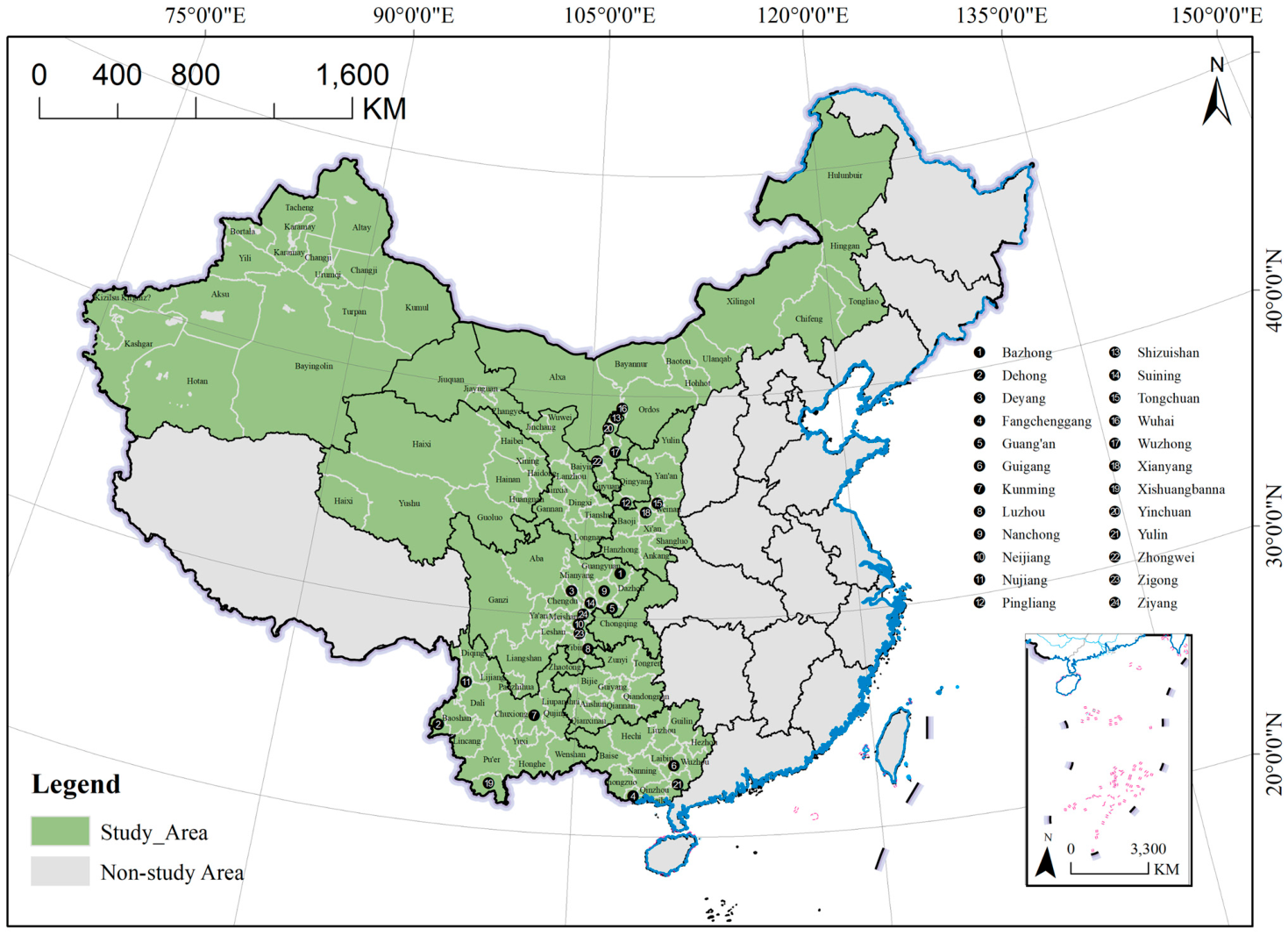
Figure 1. Study Area.
Land 15 00916 g001
Figure 2. Theoretical framework of land-use carbon emissions in rural revitalization.
Land 15 00916 g002
Figure 3. Technical routes with integrated multi-method.
Land 15 00916 g003
Figure 4. Spatial clustering and autocorrelation analysis of LUCE spatiotemporal evolution.
Land 15 00916 g004
Figure 5. Spatial clustering and autocorrelation analysis of RRI spatiotemporal evolution.
Land 15 00916 g005
Figure 6. Decoupling relationship and its spatial effect analysis.
Land 15 00916 g006
Figure 7. Dependent variable and its spatial effect analysis.
Land 15 00916 g007
Figure 8. Nature of Factor Influence.
Land 15 00916 g008
Figure 9. Intensity of Factor Influence.
Land 15 00916 g009
Figure 10. Nonlinear Paths of Factor Influence.
Land 15 00916 g010
Figure 11. Spatial heterogeneity of factor influence.
Land 15 00916 g011
Figure 12. Spatial autocorrelation of factor influence.
Land 15 00916 g012
Table 1. Indicator system for rural revitalization index.
SubsystemIndicator
Thriving
Businesses
Per Capita Total Power of Agricultural Machinery
Grain Comprehensive Production Capacity
Agricultural Labor Productivity
Main Business Income of Above-Scale Agricultural Product Processing Enterprises
Pleasant
Living
Environment
Application Number of Pesticides and Chemical Fertilizers
Comprehensive Utilization Rate of Livestock and Poultry Manure
Proportion of Administrative Villages with Domestic Sewage Treatment
Proportion of Administrative Villages with Domestic Garbage Disposal
Popularization Rate of Hygienic Toilets
Green Coverage Rate in Rural Areas
Social
Etiquette and Civility
Proportion of Rural Residents’ Expenditures on Education, Culture, and Entertainment
Proportion of Full-Time Teachers with Bachelor’s Degree or Above in Rural Compulsory Education Schools
Average Years of Schooling of Rural Residents
Cable TV Coverage Rate
Proportion of Administrative Villages with Internet Broadband Services
Number of Rural Cultural Stations
Effective
Governance
Proportion of Concurrent Position of Village Director and Party Secretary
Proportion of Administrative Villages with Compiled Village Plans
Proportion of Administrative Villages with Village Renovation Initiatives
ProsperityPer Capita Net Income of Farmers
Growth Rate of Per Capita Income of Farmers
Income Ratio between Urban and Rural Residents
Rural Poverty Incidence Rate
Engel Coefficient of Rural Residents
Car Ownership per 100 Households
Per Capita Housing Area of Rural Residents
Popularization Rate of Safe Drinking Water
Paved Road Rate in Villages
Per Capita Road Area
Number of Health Technical Personnel per 1000 Rural Residents
Table 2. Indicator system for mechanism analysis.
TypeIndicatorAbbreviationCodeVIF
Dependent VariableDecoupling Relationship Between LUCE and RRIDR Y --
Independent VariableRural PopulationRP X 1 1.48
Land Use Complexity of VillagesLUCV X 2 3.62
Population Aging IndexPAI X 3 3.22
Population Out-migration IndexPOMI X 4 2.68
Urbanization RateUR X 5 6.03
Per Capita GDP (Industrialization)PCGDP X 6 2.61
Fiscal Self-sufficiency RateFSSR X 7 3.59
Industrial Structure Rationalization IndexISRI X 8 1.09
Development Inequality IndexDII X 9 1.93
Average Years of EducationAYE X 10 5.21
Proportion of Ethnic Minority PopulationPEMP X 11 2.74
Table 3. Statistical Analysis of the Dependent Variable.
Decoupling TypesSample SizeDecoupling CategoriesSample Size
Strong Decoupling21Decoupling46
Weak Decoupling3
Recessive Decoupling22
Expansive Coupling0Coupling2
Recessive Coupling2
Expansive Negative Decoupling31Negative Decoupling76
Weak Negative Decoupling4
Strong Negative Decoupling41
Table 4. Algorithm comparison and robustness tests for explainable machine learning.
ParameterCatBoostLightGBMRandomForest
Training Accuracy1.000.931.00
Testing Accuracy0.760.720.68
Degree of Overfitting0.240.210.32
Test Precision0.730.610.59
Test Recall0.580.740.53
Test F1 Score0.650.670.56
Table 5. Threshold effects of factor influence.
AbbreviationCodeForm Negative to PositiveForm Positive to NegativeTroughPeak
X 1 RP0.050.270.650.12
X 2 LUCV0.61----0.85
X 3 PAI0.57--0.380.87
X 4 POMI--0.240.67--
X 5 UR0.50------
X 6 PCGDP0.31----0.80
X 7 FSSR0.760.230.50--
X 8 ISRI0.220.83--0.45
X 9 DII0.55----0.85
X 10 AYE0.800.630.70.9
X 11 PEMP--0.23----
Note: -- represents non-existent.
Table 6. Algorithm Comparison and Robustness Tests for Explainable Machine Learning.
AbbreviationCodeCVMoran’s IZp
X 1 RP24.10.153.720.00
X 2 LUCV10.90.4611.060.00
X 3 PAI11.70.409.570.00
X 4 POMI18.20.4510.700.00
X 5 UR8.80.297.140.00
X 6 PCGDP−16.90.153.830.00
X 7 FSSR429.00.205.000.00
X 8 ISRI25.20.112.690.01
X 9 DII−30.40.082.150.03
X 10 AYE−24.30.266.200.00
X 11 PEMP22.50.4410.460.00
Disclaimer/Publisher’s Note: The statements, opinions and data contained in all publications are solely those of the individual author(s) and contributor(s) and not of MDPI and/or the editor(s). MDPI and/or the editor(s) disclaim responsibility for any injury to people or property resulting from any ideas, methods, instructions or products referred to in the content.