The BES–GDP Nexus: A Panel Econometric and Machine Learning Analysis of Italian Regions

Abstract

The study investigates the interrelationship between the performance of the regional economy in Italy and the multidimensionality of wellbeing, as defined by the ISTAT Benessere Equo e Sostenibile (BES) model. Based on panel data from 19 Italian regions and 2 autonomous provinces—Trentino and Bolzano (2012–2023)—the research aims to explore whether there is a link between regional GDP and the three BES dimensions: Benessere (B), Equità (E), and Sostenibilità (S). The innovative contribution of this paper is not the creation of a novel theoretical model, but a multilayered empirical approach that combines panel data methods, machine learning, and clustering. This approach makes it possible to reveal nonlinearities, complex interactions, and regional heterogeneity in BES–GDP relationships. The analysis of the Benessere dimension based on k-Nearest Neighbors reveals nonlinear dynamics related to health, mobility, security, digital access, and socio-economic conditions. Furthermore, cluster analysis identifies territorial development regimes according to the Benessere dimension. The Equità dimension is estimated using boosting regression and clustering models that emphasize the role of income, poverty risk, healthcare pressure, labour-market participation, youth exclusion, deprivation, and access to essential services. Finally, the Sostenibilità dimension is explored using boosting regression and random forest models to estimate interactions among environmental quality, climate stress, energy transition, innovation, digital skills, service reliability, and regional economic performance. The findings demonstrate a structural connection between well-being, equity, sustainability, and the economic performance of Italian regions. The results also confirm the hypothesis that Italy has multiple development regimes that differ geographically.

1. Introduction

Economic performance has long been assessed primarily through Gross Domestic Product (GDP). However, its limitations in capturing broader dimensions of development and well-being are now widely recognized [1]. GDP does not account for income distribution, environmental externalities, institutional quality, or sustainability, and economic growth may coexist with inequality, environmental degradation, and declining quality of life [2]. This disconnect is particularly evident in advanced economies, where increases in GDP do not necessarily translate into improvements in living standards or well-being [3,4]. In response, multidimensional frameworks have been developed to provide a more comprehensive assessment of socio-economic development [1]. Among these, the Italian Benessere Equo e Sostenibile (BES) framework offers a structured approach that integrates social, economic, institutional, and environmental dimensions, including health, education, security, income, and sustainability [5]. Despite its conceptual relevance, BES has been predominantly used for descriptive purposes, and its relationship with economic performance remains underexplored [5].

This study addresses this gap by examining the association between BES and regional GDP in Italy. Specifically, we focus on three core dimensions—Benessere (B), Equità (E), and Sostenibilità (S)—and analyze how they relate to economic performance across regions. This perspective is particularly relevant in the Italian context, characterized by persistent territorial disparities between more developed northern regions and structurally weaker southern areas. This study addresses this gap by examining the association between BES and regional GDP in Italy. In doing so, it explicitly adopts a territorial perspective, aiming to analyze regional disparities and spatial heterogeneity in well-being, equity, and sustainability across Italian regions, and to better understand the drivers of uneven development patterns.

Existing literature typically examines economic, social, and environmental drivers of growth separately, while often relying on linear models that overlook non-linear relationships and regional heterogeneity [2,3]. In contrast, this paper adopts an integrated approach that combines panel econometrics, machine learning, and clustering techniques to jointly capture structural relationships, non-linear dynamics, and territorial differences. To the best of our knowledge, this combination has not yet been applied to the analysis of the BES–GDP nexus in Italy.

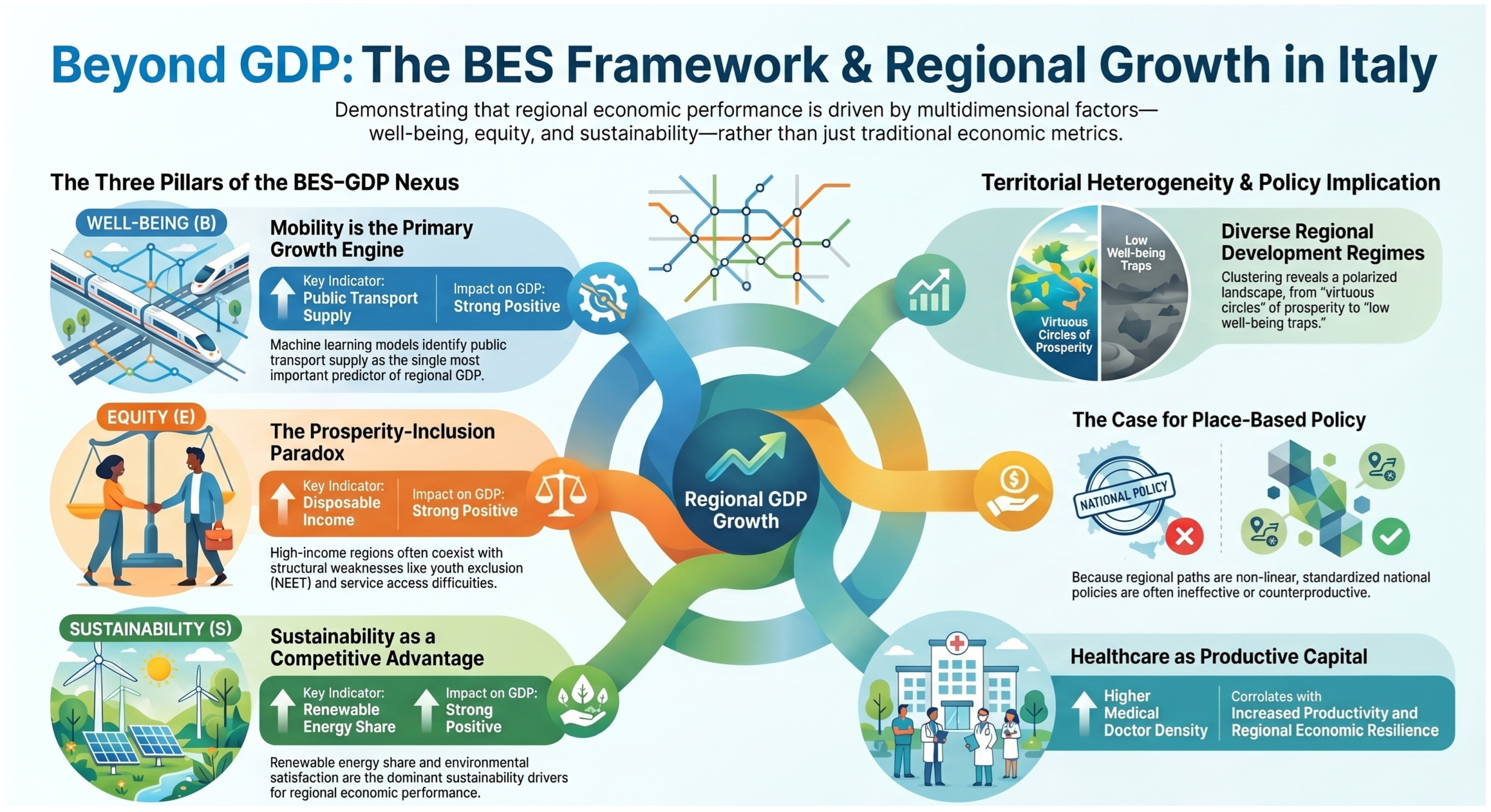
The contribution of the study is threefold. First, it provides new empirical evidence on the relationship between multidimensional well-being and regional economic performance. Second, it introduces a methodological framework that integrates complementary analytical tools to better capture the complexity of socio-economic systems. Third, by distinguishing between the three BES dimensions (B, E, and S), it allows a more detailed assessment of their individual roles in shaping economic outcomes. It is important to clarify that the originality of this study does not consist in proposing a new theory of economic development. Rather, its novelty is empirical and methodological, as it combines panel econometrics, machine learning, and clustering analysis within the BES framework to capture nonlinear relationships, complex interactions, and territorial heterogeneity in the BES–GDP nexus.

Overall, the analysis is grounded in the view that well-being constitutes a fundamental dimension of economic performance [1]. The BES framework is therefore used as an interpretative structure to examine how social, institutional, and environmental factors interact with economic dynamics. In this context, the study aims to provide a clearer and more concise interpretation of the relationship between well-being, equity, sustainability, and regional GDP.

The remainder of the paper is organized as follows. Section 2 reviews the literature, and Section 3 presents the methodology. Section 4, Section 5 and Section 6 analyze the three BES dimensions—Benessere, Equità, and Sostenibilità—and their relationship with regional GDP. Section 7 provides an integrated interpretation of the results, while Section 8 discusses the role of social, institutional, and environmental factors. Section 9 presents the discussion of the results, and Section 10 outlines the policy implications. Section 11 concludes. Additional results and technical details are provided in Appendix A, Appendix B, Appendix C, Appendix D and Appendix E.

2. Literature Review

Contemporary research consistently emphasizes a fundamental principle: economic growth should be studied in conjunction with social well-being, institutions, and sustainability, consistent with the BES approach and sustainable growth theories. In addition, several recent studies suggest that natural resources and environmental policies positively affect economic performance provided their integration into proper institutional and innovative contexts [6,7,8,9,10,11,12,13,14]. Moreover, energy security, infrastructure reliability, and climatic risks are essential determinants of long-run growth dynamics [15,16]. The importance of human welfare as a production factor is another significant conclusion. Health status, environment, and subjective satisfaction have a direct impact on productivity and economic performance [17,18,19,20,21,22]. The role of institutions and governance in shaping the relationship between social factors and economic development is highlighted due to their effects on economic freedom, welfare, and policy implementation [23,24,25]. These studies clearly indicate the need to go beyond GDP and adopt a multidimensional approach to development [26,27]. Several recent works also question the adequacy of GDP as the main measure of prosperity, proposing redistribution, resilience, and social cohesion as alternatives for explaining development [28,29,30,31]. Within the context of regions, social capital, culture, and civic participation are shown to have a great impact on economic results [32,33]. At the same time, territorial features, infrastructural facilities, and geography significantly determine development paths [34,35,36]. Demographic trends and inequality are among the most relevant issues in contemporary economics. Aging, migration, and human capital accumulation have a considerable effect on productivity and long-term growth [37,38,39,40]. Furthermore, poverty and inequality should be treated as multidimensional phenomena [41,42,43,44]. Finally, technological innovation and sustainability transitions, including digitalization, green finance, and renewable energy, emerge as important factors linked to growth and inclusiveness. However, such processes usually involve trade-offs regarding social and environmental aspects [45,46,47,48,49]. See

Table 1. Integrating the Multidimensional Determinants of Growth: Macro-Themes from the Literature and Their Link to the BES Framework.

Macro-Theme	Core Idea	Key Contributions from the Literature	Link with BES Framework
Environment & sustainability	Natural resources, energy systems and climate risks shape long-term growth	[6,7,8,16,49].	Environment and sustainability as structural drivers of GDP
Social well-being & human capital	Health, well-being, education and demographic factors influence productivity and growth	[17,18,20,25,40].	Well-being and human capital as inputs in GDP generation
Institutions & equity	Governance, inequality, poverty and inclusion shape development paths	[23,24,41,42].	Institutional quality and equity explain regional divergence
Social & territorial dynamics	Social capital, participation, geography and infrastructure affect economic outcomes	[27,32,34,35].	Social cohesion and territorial factors explain GDP heterogeneity
Innovation & development models	Innovation, finance and post-growth approaches redefine economic development	[28,29,45,48].	BES as a multidimensional alternative to GDP

Note: This table links key economic, social, and environmental drivers—such as health, institutions, equity, and innovation—to BES dimensions, showing how they act as structural inputs shaping long-term regional economic performance.

.

3. Methodology

The interrelation between well-being and economic growth is complex, multifaceted, and heterogeneous across space, as social inclusion, environmental sustainability, innovation, public services, and institutions influence GDP through nonlinear channels [50,51,52]. For this reason, the current research uses the combined empirical methodology comprising panel econometrics, machine-learning regression, and clustering. Panel econometric models are employed to examine the dynamic correlation between GDP and various well-being indicators, while controlling for unobserved region-specific heterogeneity using fixed- and random-effects approaches [50]. In this case, we obtain a structural interpretation of the relationship under investigation, but this approach relies on the assumption of linearity, which does not capture all nuances of socio-economic systems [53]. Machine-learning algorithms can help us detect non-linearities and relationships within the data [54,55]. In particular, the application of K-Nearest Neighbors is suggested to measure local similarity between regions with respect to the Benessere dimension. The Boosting algorithm is proposed for use with the Equità and Sostenibilità dimensions due to its high predictive accuracy and its ability to model interactions between variables [52]. Model performance will be measured using normalized statistics such as R², RMSE, and MAE [53]. To ensure the estimates are reliable, the dataset will be randomly split into training and test subsets, and hyperparameter tuning will be performed via validation procedures to prevent overfitting [54]. The hyperparameter configuration and data splitting procedures for the machine-learning models are reported in Appendix E. All details about models’ specification, validation, and evaluation can be found in the Appendixes. Finally, the clustering technique will allow us to identify territorial development regimes, i.e., groups of regions with similar BES-GDP profiles. It should be noted that our study uniformly applies clustering across all BES dimensions to ensure comparability and transparency. For the Benessere and Equità dimensions, hierarchical clustering will be carried out using standardized variables (i.e., z-scores), Euclidean distance, and Ward’s linkage criterion, which minimizes within-cluster variance [50,51]. The number of clusters will be selected based on several statistical criteria, including the Bayesian Information Criterion (BIC), the within-cluster sum of squares (WSS), and a graphical analysis of the dendrogram. As for the Sostenibilità dimension, the use of clustering based on a proximity matrix generated with Random Forest will enable the detection of complex patterns, including non-linear similarities between observations and interactions among variables. All in all, each method serves its purpose. So, panel econometrics helps discover structural associations; machine learning is useful for uncovering nonlinearities and prediction; and clustering shows the spatial diversity of well-being. The choice of this methodological combination reflects the innovative nature of the current study, as all three aspects of the BES-GDP relationship will be considered simultaneously. The methodology is described here to prevent repetition in the empirical sections of the paper [56,57]. Thus, the results section only concerns the interpretation of empirical results. See Figure 1.

The dataset includes 21 Italian territorial units—19 regions and the Autonomous Provinces of Trento and Bolzano—over the period 2012–2023. This level of disaggregation allows the analysis to capture the territorial heterogeneity of the Italian economy [58,59]. GDP dynamics show an overall upward trend, interrupted by a contraction in 2020 due to the COVID-19 pandemic and followed by a recovery in 2021–2023 [60,61].

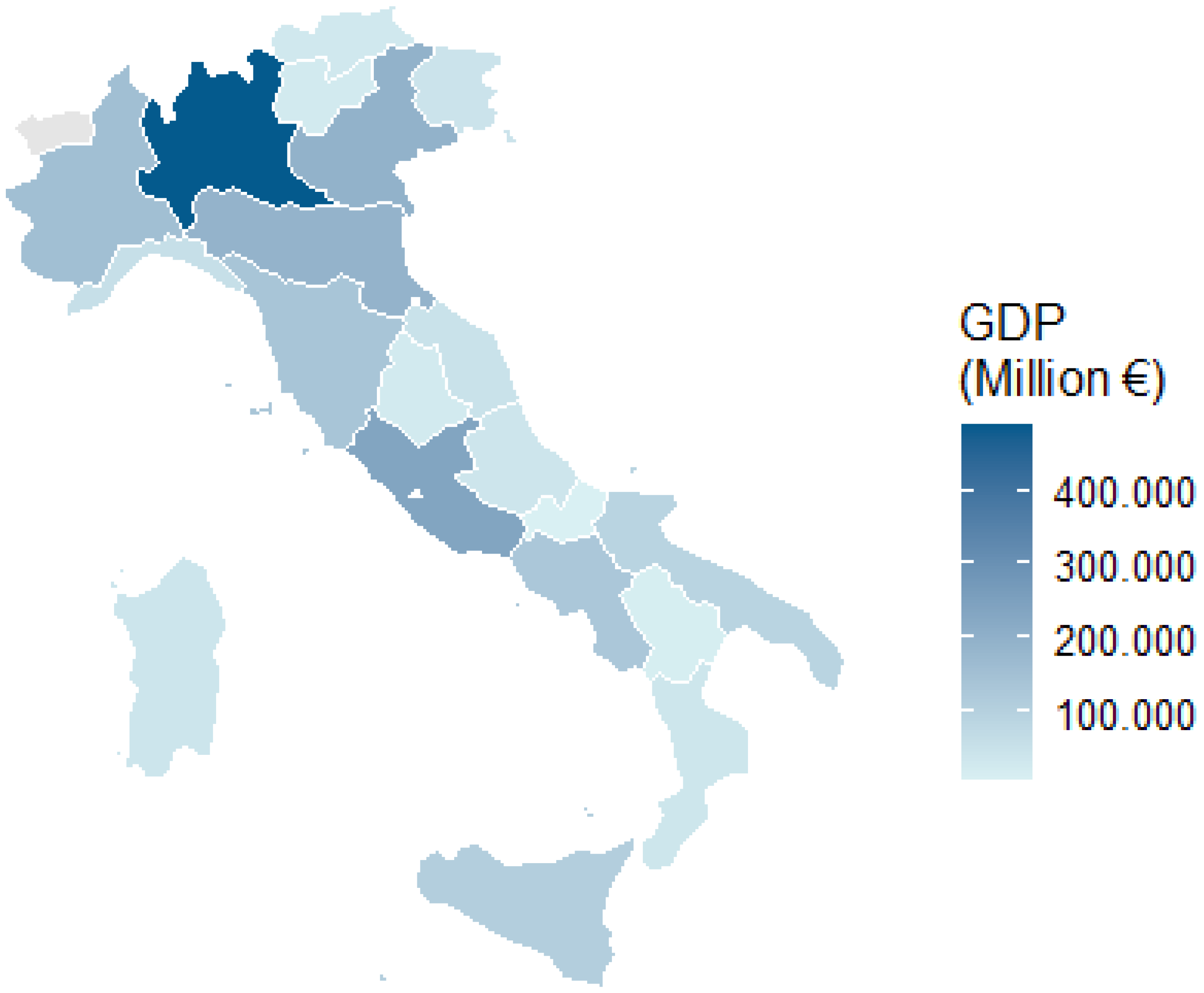
At the same time, significant regional disparities persist, with higher economic concentration in northern regions such as Lombardy, Veneto, and Emilia-Romagna, intermediate performance in central regions, and lower GDP levels in southern regions and islands [62]. These territorial differences highlight the structural heterogeneity of the Italian economy and provide the empirical motivation for adopting a multidimensional framework such as BES to interpret the relationship between well-being and economic performance. The spatial distribution of GDP is illustrated in Figure 2.

The following table summarizes all variables used throughout the article within the BES framework, grouped according to the three main dimensions—Benessere (B), Equità (E), and Sostenibilità (S)—together with the dependent variable GDP. For each indicator, the corresponding acronym and a brief description are reported to improve readability, methodological transparency, and consistency across the empirical analyses conducted in the study. See

Table 2. BES Variables, Acronyms, and Descriptions Used in the Empirical Analysis.

BES	Acronym	Variable	Description
B	CPP	Civic Political Participation	Participation in civic and political activities
	DFLE	Disability-Free Life Expectancy at Age 65	Expected years of life without disability at age 65
	HBR	Home Burglary Rate	Residential burglaries per population (security indicator)
	HDA	Household Digital Access	Access of households to digital technologies and internet connectivity
	HLEB	Healthy Life Expectancy Birth	Expected years of healthy life at birth
	MDD	Medical Doctors Density	Doctors per population (healthcare access indicator)
	OHCP	Cultural participation outside the home	Participation in cultural activities outside home
	PTS	Public Transport Supply	Availability of public transport seat-kilometers
	PTS2	Satisfaction with public transport services	Degree of satisfaction with public transport quality
	RIU	Regular Internet Users	Share of population regularly using the internet
	RR	Robbery Rate	Incidence of robberies (personal safety indicator)
E	GDIPC	Gross Disposable Income per Capita	Average disposable income (purchasing power indicator)
	GPO	General Practitioners Overload	General practitioners exceeding patient threshold
	LMNP	Labour market non-participation	Share of population excluded from labour market participation
	MEGR	Employment rate	Proportion of employed individuals within the working-age population
	PRR	Poverty risk rate	Share of population at risk of poverty or social exclusion
	SAD	Service Access Difficulty	Population reporting difficulty accessing essential services
	SHD	Severe material and social deprivation	Lack of essential material and social resources
	YNEE	Youth Not in Employment, Education or Training	Share of youth not in employment, education, or training
S	BLC	Biodiversity Loss Concern	Concern about biodiversity loss and ecosystem degradation
	CCC	Climate Change Concern	Degree of public concern about climate change
	DSD	Digital Skills Deficit	Share of the population with insufficient digital skills
	ESI	Irregularities in the electrical service	Frequency of disruptions in electrical service availability
	ESL	Environmental Satisfaction Level	Degree of satisfaction with environmental quality
	HDI	Heatwave Duration Index	Measures duration and intensity of heatwaves (climate stress)
	PAC	Protected Area Coverage	Extent of protected natural areas within the region
	PPI	Patent Propensity Index	Tendency of firms to generate patents
	RES	Renewable Energy Share	Share of energy produced from renewable sources
	RII	Research and Innovation Intensity	Indicator of regional research and innovation activity
	SWC	Separate Waste Collection	Indicator measuring municipal separate waste collection services
	WSI	Water Service Interruption	Indicator of reliability/continuity of water services
Y	GDP	Gross Domestic Product	Total economic output and income of a region

Note. This table reports the variables employed in the empirical analysis of the BES–GDP nexus. Indicators are grouped according to BES dimensions and include acronyms and concise descriptions to ensure methodological consistency, transparency, and interpretability throughout the econometric and machine-learning analyses.

.

4. From Quality of Life to Economic Output: The Benessere–GDP Nexus

This chapter examines the relationship between well-being indices and regional GDP in Italy. The main focus will be on security, service availability, and health care as the primary determinants of economic performance, assessing whether an improvement in well-being leads to increased economic productivity.

Specifically, we have estimated the following equation:

$$\mathrm{G}\mathrm{D}{\mathrm{P}}_{\mathrm{i}\mathrm{t}}=\mathsf{\alpha }+{\mathsf{\beta }}_1{\left(\mathrm{H}\mathrm{B}\mathrm{R}\right)}_{\mathrm{i}\mathrm{t}}+{\mathsf{\beta }}_2{\left(\mathrm{R}\mathrm{R}\right)}_{\mathrm{i}\mathrm{t}}+{\mathsf{\beta }}_3{\left(\mathrm{P}\mathrm{T}\mathrm{S}\right)}_{\mathrm{i}\mathrm{t}}+{\mathsf{\beta }}_4{\left(\mathrm{M}\mathrm{D}\mathrm{D}\right)}_{\mathrm{i}\mathrm{t}}$$

where i = 21 and t = 2012–2023.

The panel regression examines the association between regional GDP and selected BES well-being indicators, including security (burglary and robbery), access to services (public transport), and healthcare (medical doctor density). The results indicate that a fixed-effects specification is appropriate, confirming the presence of significant territorial heterogeneity [63,64]. Empirical findings show a negative relationship between crime rates and GDP, and a positive association with transport availability and healthcare access. These results suggest that mobility and health represent key components of regional economic performance, in line with previous studies [65]. Diagnostic issues such as heteroskedasticity, autocorrelation, cross-sectional dependence, residual normality, Hausman specification, and group effects are summarized in Appendix D. Overall, the model shows good explanatory power, confirming that well-being indicators are significantly associated with regional GDP [66]. See

Table 3. Fixed-Effects and Random-Effects Estimates of the B–Benessere Determinants of Regional GDP in Italy (2012–2023).

Variable	FE Coef.	FE Std. Err.	FE t	RE Coef.	RE Std. Err.	RE z
Constant	−5626.07	19,888.6	−0.28	−5468.28	25,804.3	−0.21
HBR	−958.31 ***	203.07	−4.72	−987.79 ***	200.81	−4.92
RR	−4962.09 ***	1766.13	−2.81	−4939.55 ***	1752.75	−2.82
PTS	11.30 ***	1.58	7.17	12.14 ***	1.54	7.91
MDD	16,575.9 ***	4950.4	3.35	15,914.6 ***	4867.83	3.27

Note: *** p < 0.01. FE = Fixed Effects; RE = Random Effects. Full diagnostic tests and additional statistics are reported in Appendix A. The dependent variable is GDP (Gross Domestic Product). The explanatory variables included in the model are: HBR (Home Burglary Rate), RR (Robbery Rate), PTS (Public Transport Supply), and MDD (Medical Doctors Density). These variables capture dimensions related to security, mobility, and healthcare access within the BES Benessere framework.

.

4.1. Modeling the Benessere–GDP Nexus with Machine Learning: Evidence from KNN

The KNN results highlight nonlinear relationships between well-being indicators and regional GDP. Beyond prediction, the model provides insights into the relative importance of different well-being dimensions in explaining regional economic performance. The results reveal heterogeneous local patterns across regions [67,68]. These results are consistent with previous studies showing that nonlinear models improve the detection of complex socio-economic interactions [69].

The KNN feature importance analysis shows that mobility is the most relevant predictor of regional GDP, followed by health and security. In contrast, digitalization and social participation play a more limited role. These results highlight the importance of core well-being dimensions—particularly transport accessibility, healthcare, and safety—in shaping regional economic performance, in line with previous findings [67,68]. See

Table 4. KNN Feature Importance of B–Benessere Indicators in Explaining Regional GDP.

Variables	PTS	PTS2	HBR	MDD	DFLE
Mean Dropout Loss	82,406	35,332	31,932	30,054	25,475
Variables	HLEB	CPP	RIU	OHCP	HDA
Mean Dropout Loss	23,649	23,553	23,072	21,837	20.89

Note. This table reports KNN mean dropout losses for BES Benessere indicators. Higher values indicate greater importance in explaining regional GDP, showing that mobility, security, health, digital access, and social participation are key factors associated with Italian economic performance.

.

The KNN decomposition confirms that mobility and security have the strongest impact on regional GDP, with poor transport infrastructure and higher crime rates significantly reducing economic output. Health also contributes to GDP, although with more heterogeneous effects across regions. In contrast, digitalization and social participation play a secondary role. These findings further support the relevance of core well-being dimensions in shaping regional economic performance [70,71].

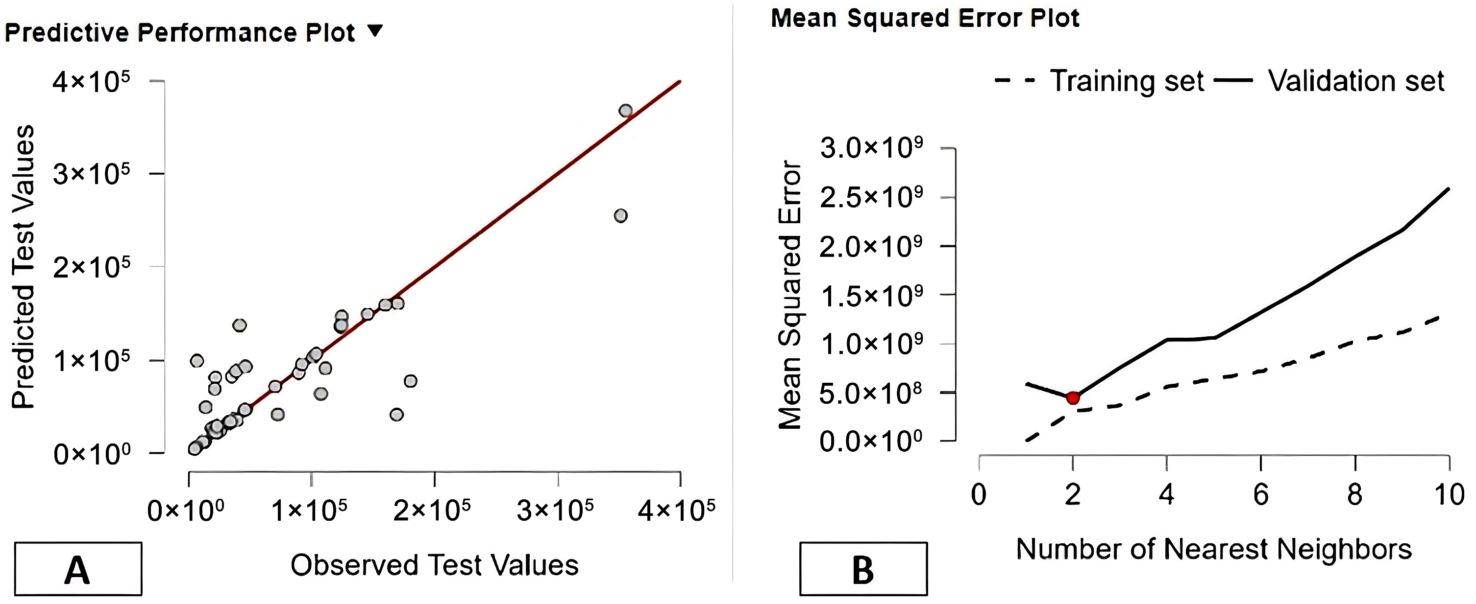
Figure 3 shows the predictive performance of the KNN model. Predictions are more accurate for regions with low and medium GDP, while greater dispersion is observed for higher-income regions. Overall, the results indicate that KNN captures nonlinear and heterogeneous relationships between well-being indicators and regional GDP [72,73,74]. See Figure 3.

4.2. Territorial Patterns of Benessere and Economic Performance in Italy

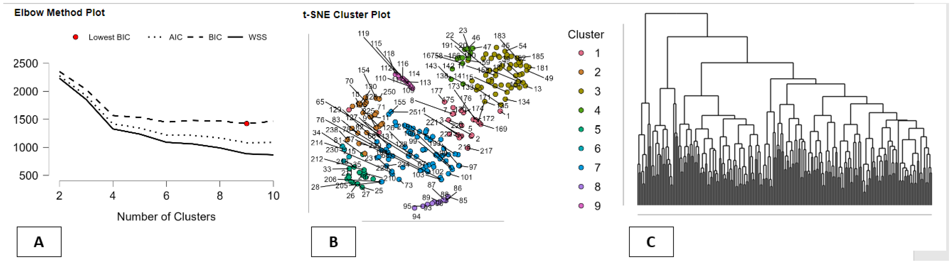
The clustering results identify stable and well-defined groups that reflect underlying patterns in the data. Moreover, the clusters reveal meaningful differences in economic and well-being indicators, allowing the identification of distinct regional development regimes [75,76,77,78,79]. z-scores are reported in standardized form, where positive values indicate above-average performance and negative values indicate below-average performance. The results reveal substantial heterogeneity in the relationship between GDP and multidimensional well-being across Italian regions. In particular, some clusters are characterized by low GDP and weak performance across key well-being dimensions, while others combine high economic output with strong outcomes in health, security, and mobility. Intermediate clusters display more balanced or mixed profiles, suggesting different combinations of economic and social characteristics. Overall, the findings indicate that regional development does not follow a single trajectory but rather multiple distinct paths, reflecting diverse configurations of well-being and economic performance. This evidence is consistent with recent studies on territorial heterogeneity and cluster-based development patterns [80,81,82,83,84]. These results highlight the importance of designing policies tailored to the specific characteristics of regional clusters (see

Table 5. Hierarchical Clustering Profiles of GDP and B–Benessere in Italian Regions.

Cluster	GDP	HLEB	DFLE	OHCP	CPP	HBR	RIU	HDA	PTS	PTS2	MDD
1	0.12	−0.49	−0.58	−0.13	−0.07	−0.60	1.15	0.07	−0.30	0.09	−0.31
2	0.55	0.39	−0.14	−0.63	0.91	0.60	0.68	−1.10	−0.24	0.35	1.28
3	−1.31	−1.12	−0.31	−0.47	−1.27	−0.98	−0.19	−0.54	−0.72	−0.64	−0.99
4	−1.26	−0.75	−0.37	−1.22	−0.23	−0.48	0.04	−1.91	−0.83	0.01	0.64
5	0.41	0.72	−0.68	−0.41	1.16	2.12	−1.57	1.44	0.14	2.02	0.55
6	0.94	1.30	−0.65	−1.14	1.93	1.98	−1.18	−0.95	0.38	2.33	1.82
7	0.66	0.63	0.01	0.82	0.10	0.18	−0.18	0.59	0.06	−0.07	−0.06
8	0.40	−0.06	1.29	−0.02	0.65	−0.06	1.58	0.69	1.63	−1.18	0.41
9	0.48	0.79	3.44	0.92	0.86	0.17	−0.58	0.43	3.24	−0.08	0.58

Note. This table reports standardized cluster means (z-scores) for GDP and BES Benessere indicators. Positive values indicate above-average performance. The clusters reveal distinct territorial development regimes, ranging from low well-being–low GDP traps to virtuous circles of prosperity, health, mobility, and social capital.

).

Figure 4 illustrates the clustering results, highlighting the presence of distinct territorial groups among Italian regions. The identified clusters confirm the existence of different development regimes linking well-being and GDP. See Figure 4.

5. Equity, Inclusion and Regional Growth: Evidence from Italian Panel Data

This section analyzes the relationship between equity-related BES indicators and regional GDP, focusing on income, youth exclusion, and access to services. The aim is to assess whether social inclusion and opportunity structures are systematically associated with economic performance across Italian regions over the period 2012–2023. Specifically, we have estimated the following equation:

$$\mathrm{G}\mathrm{D}{\mathrm{P}}_{\mathrm{i}\mathrm{t}}=\mathsf{\alpha }+{\mathsf{\beta }}_1{\left(\mathrm{Y}\mathrm{N}\mathrm{E}\mathrm{E}\right)}_{\mathrm{i}\mathrm{t}}+{\mathsf{\beta }}_2{\left(\mathrm{G}\mathrm{D}\mathrm{I}\mathrm{P}\mathrm{C}\right)}_{\mathrm{i}\mathrm{t}}+{\mathsf{\beta }}_3{\left(\mathrm{S}\mathrm{A}\mathrm{D}\right)}_{\mathrm{i}\mathrm{t}}$$

where i = 21 and t = 2012–2023.

Model selection results indicate that the random-effects specification is preferred over fixed effects and pooled OLS, suggesting that unobserved regional differences do not bias the estimates. The results show a positive association between disposable income and GDP, confirming its central role in economic performance. At the same time, youth exclusion (NEET) and service-access difficulties (SAD) are also positively correlated with GDP. These relationships likely reflect structural characteristics of more developed regions rather than causal effects of inequality, as higher-income areas may exhibit delayed labor-market entry and greater congestion. Overall, the findings highlight a multidimensional relationship between growth and social conditions, where economic performance may coexist with inequality and access constraints. These results are consistent with recent studies on the complex link between income, inequality, and regional development [85,86,87,88,89]. See

Table 6. Fixed-Effects and Random-Effects Estimates of E–Equo Determinants of Regional GDP in Italy (2012–2023).

Variable	FE Coefficient	FE Std. Error	FE t	RE Coefficient	RE Std. Error	RE z
Constant	−75,703.2 ***	19,845.0	−3.82	−77,092.9 ***	27,540.1	−2.80
YNEE	533.69 **	212.88	2.51	545.35 ***	211.66	2.58
GDIPC	7.47 ***	0.80	9.32	7.52 ***	0.79	9.46
SAD	1142.19 **	509.29	2.24	1156.22 **	506.66	2.28

Note. *** p < 0.01, ** p < 0.05. The dependent variable is regional GDP, estimated using a panel of 21 Italian regions over the period 2012–2023.

.

5.1. Social Equity and Growth: Evidence from a Boosting Model

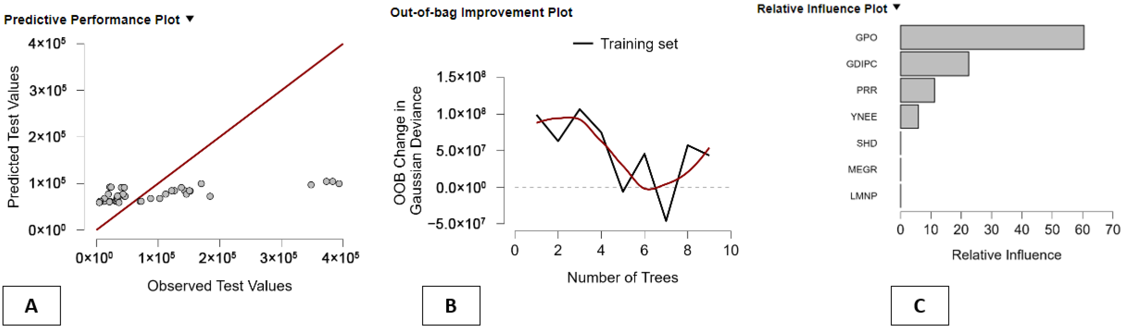
The boosting regression highlights the relative importance of E–Equo variables in explaining regional GDP. General Practitioners Overload (GPO) emerges as the most relevant predictor, followed by disposable income (GDIPC) and poverty risk rate (PRR), which shows an inverse relationship with GDP. Youth exclusion (YNEE) has a more limited but still relevant role, while other variables (LMNP, MEGR, SHD) contribute marginally. Overall, the results indicate that healthcare pressure, income conditions, and poverty dynamics are the main channels linking equity to economic performance within the BES framework. These findings are consistent with recent studies using boosting methods to assess the relative importance of socio-economic factors [90,91,92]. See

Table 7. Boosting Feature Importance of E–Equo BES Indicators in Explaining Regional GDP.

Variable	Relative Importance	Normalized Dropout Loss
GPO	1.00	1.00
GDIPC	0.37	0.96
PRR	0.19	0.95
YNEE	0.01	0.95
LMNP	0.00	0.94
MEGR	0.00	0.94
SHD	0.00	0.94

Note. Values are reported in normalized form to enhance readability and facilitate comparison across variables. Higher values indicate a greater contribution to the predictive performance of the model. The results highlight the dominant role of General Practitioners Overload, disposable income, and poverty risk, while other variables contribute only marginally to explaining regional GDP. Full results in absolute values are provided in Appendix B.

.

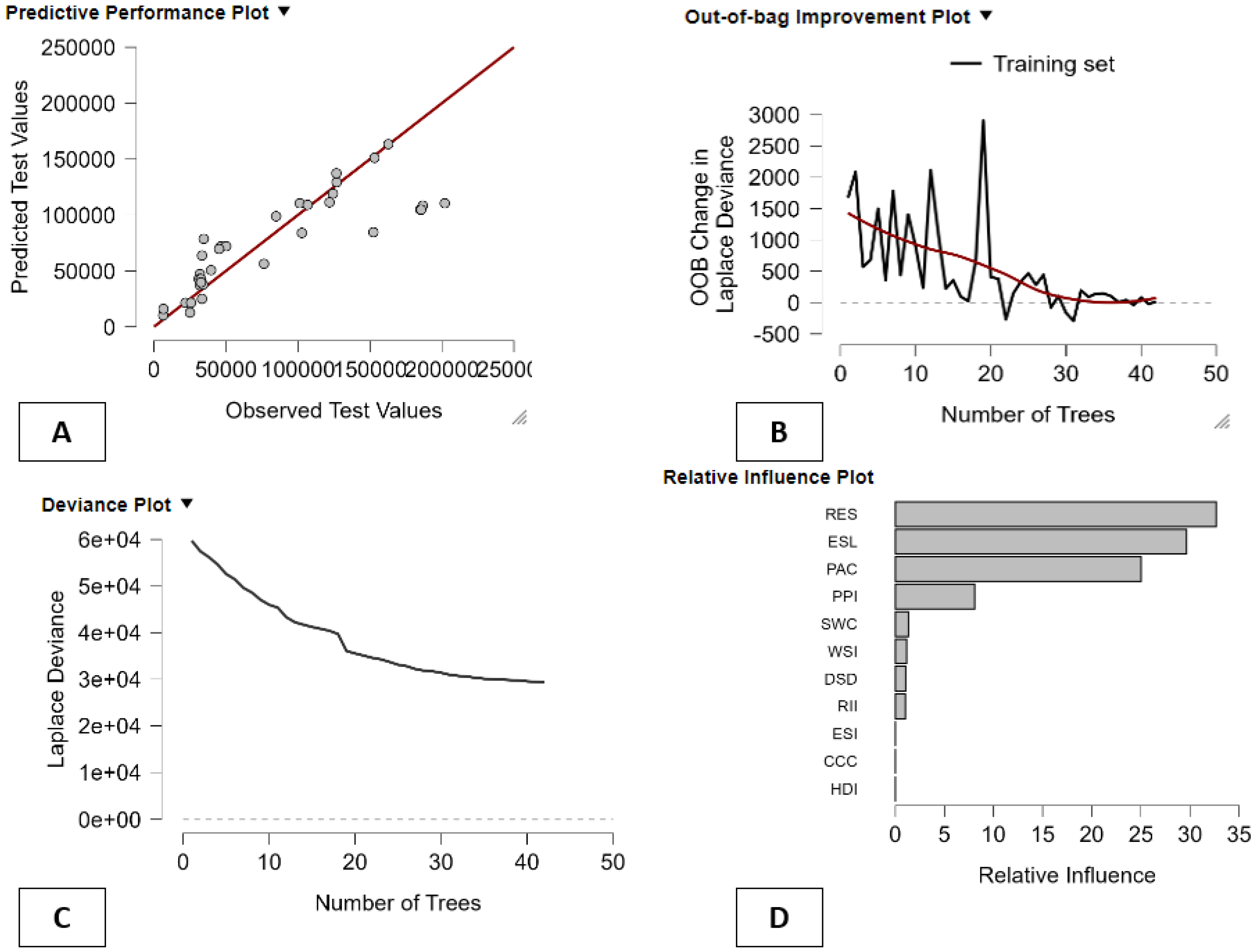
Figure 5 summarizes the performance of the Boosting model. Panel A shows good predictive accuracy, particularly for regions with lower GDP, while larger dispersion emerges for higher-income regions. Panel B indicates that model performance stabilizes after a limited number of trees. Panel C highlights that GPO, GDIPC, and PRR are the main predictors of GDP. These findings confirm that healthcare pressure, disposable income, and poverty risk drive most of the model’s predictive performance within the E–Equo dimension [93,94]. See Figure 5.

5.2. How Clustering Reveals the Structure of the E-Equo–GDP Relationship

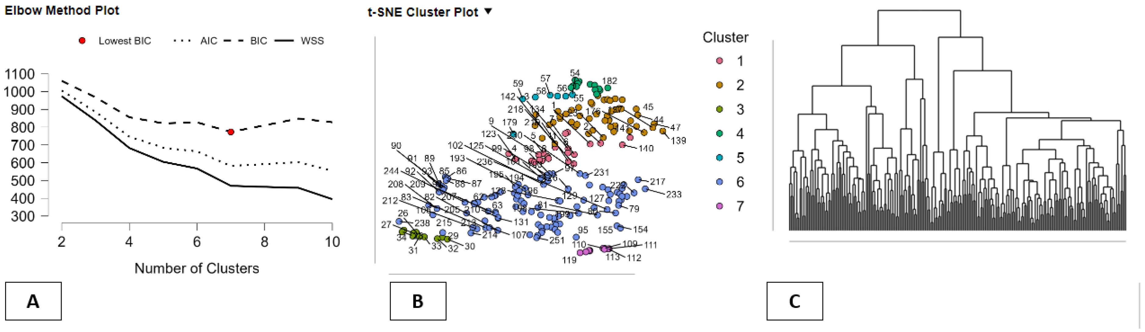
The E–Equo clustering analysis identifies distinct territorial profiles based on disposable income, poverty risk, healthcare pressure, labour-market participation, employment, youth exclusion, material and social deprivation, and access to essential services [95,96,97]. The hierarchical clustering results reveal substantial heterogeneity in the relationship between the E–Equo dimension and regional GDP across Italy. Some clusters combine high GDP with stronger income and employment conditions, while others show economic performance alongside healthcare overload or social vulnerability. At the opposite end, several clusters are characterized by low GDP and weak performance in key equity indicators, including poverty risk, labour-market exclusion, youth exclusion, deprivation, and service-access difficulty. Intermediate clusters display mixed profiles, reflecting uneven development patterns across territories. Overall, the results point to clear polarization between more advanced and structurally disadvantaged regions, confirming significant territorial disparities in the link between equity and economic performance [98,99]. See

Table 8. Hierarchical Clustering Profiles of E–Equo and GDP in Italian Regions.

Clusters	GDP	GDIPC	GPO	PRR	YNEE	LMNP	MEGR	SHD
1	−0.51	−0.62	−0.73	0.04	0.65	0.10	1.27	−0.00
2	−1.10	−0.49	−0.84	1.04	−0.44	1.03	−0.16	0.88
3	1.78	−0.69	2.11	−1.36	−0.71	−1.13	0.03	−1.26
4	−1.57	−0.08	−0.81	2.05	−2.17	1.76	1.81	2.27
5	−1.02	0.18	0.71	1.26	−2.14	1.77	0.08	0.95
6	0.60	0.07	0.23	−0.63	0.54	−0.66	−0.37	−0.57
7	1.18	3.40	1.69	−0.83	0.18	−0.78	−0.44	−0.74

Note. This table reports standardized cluster means for GDP and BES E–Equo indicators. Positive values denote above-average performance. The clusters reveal strong territorial polarization, distinguishing regions with stronger income and employment conditions from areas characterized by poverty risk, labour-market non-participation, youth exclusion, severe material and social deprivation, healthcare overload, and difficulty accessing essential services.

.

Figure 6 illustrates the clustering results, highlighting well-defined territorial groups based on E–Equo indicators, including disposable income, healthcare overload, labour-market participation, employment, poverty risk, service access difficulty, deprivation, and youth exclusion. The identified clusters reveal heterogeneous relationships between equity conditions and regional GDP, supporting the existence of distinct territorial regimes [100,101,102]. See Figure 6.

6. GDP and the Sustainability Dimension of the BES Framework

The relationship between economic development and environmental sustainability is a central component of the BES framework, which considers both environmental conditions and awareness alongside GDP. This study examines the association between three key indicators—Heatwave Duration Index, Climate Change Concern, and Biodiversity Loss Concern—and regional GDP in Italy over the period 2012–2023. The analysis investigates whether environmental stress and environmental awareness are merely outcomes of economic growth or represent structural elements of the development process [103,104,105,106,107,108,109]. Specifically, we have estimated the following equation:

$$\mathrm{G}\mathrm{D}{\mathrm{P}}_{\mathrm{i}\mathrm{t}}=\mathsf{\alpha }+{\mathsf{\beta }}_1{\left(\mathrm{H}\mathrm{D}\mathrm{I}\right)}_{\mathrm{i}\mathrm{t}}+{\mathsf{\beta }}_2{\left(\mathrm{C}\mathrm{C}\mathrm{C}\right)}_{\mathrm{i}\mathrm{t}}+{\mathsf{\beta }}_3{\left(\mathrm{B}\mathrm{L}\mathrm{C}\right)}_{\mathrm{i}\mathrm{t}}$$

where i = 21 and t = 2012–2023.

The panel analysis examines the relationship between regional GDP and three sustainability indicators—Heatwave Duration Index, Climate Change Concern, and Biodiversity Loss Concern—over 2012–2023. Model selection supports a random-effects specification. All indicators are positively and significantly associated with GDP, with the strongest relationship observed for climate change concern and a weaker effect for biodiversity concern. These coefficients reflect structural associations rather than causal effects, as more developed regions tend to be both more exposed to environmental pressures and more aware of environmental issues. Overall, the results suggest that environmental stress and awareness evolve alongside economic development, making sustainability an endogenous component of the growth process [110,111,112,113,114]. See

Table 9. Fixed-Effects and Random-Effects Estimates of Sustainability (S) Determinants of Regional GDP in Italy (2012–2023).

Variable	FE Coefficient	FE Std. Error	FE t	RE Coefficient	RE Std. Error	RE z
Constant	29,321.0 ***	9729.6	3.01	29,250.8	22,862.1	1.28
HDI	274.44 ***	56.60	4.85	274.64 ***	56.38	4.87
CCC	599.41 ***	189.35	3.17	600.76 ***	188.56	3.19
BLC	450.42 *	259.65	1.74	449.37 *	258.49	1.74

Note. *** p < 0.01, * p < 0.10. The dependent variable is regional GDP, estimated using a panel of 21 Italian regions over the period 2012–2023. Results indicate a positive association between sustainability-related factors and economic performance.

.

6.1. Machine Learning Insights into Sustainable Economic Performance

The results indicate that sustainability-related variables play a relevant role in explaining regional GDP differences. Other approaches, including Decision Trees, KNN, and Random Forest, exhibit weaker performance across these metrics. These results confirm the effectiveness of boosting methods in improving predictive accuracy by combining multiple learners [115,116,117]. A limited set of variables—Renewable Energy Share (RES), Environmental Satisfaction (ESL), and Protected Area Coverage (PAC)—accounts for most of the model’s predictive power, with RES emerging as the dominant factor. These findings suggest that renewable energy, environmental quality, and ecosystem protection are key components of regional economic performance, while other sustainability indicators play a marginal role. This evidence is consistent with recent studies highlighting the importance of green growth and environmental quality in economic development [118,119,120]. See

Table 10. Normalized Feature Importance of Sustainability (S) BES Indicators in Explaining Regional GDP.

Feature	PAC	RES	ESL	PPI	SWC	WSI	DSD	RII	HDI	CCC	ESI
Relative Importance	0.76	1.00	0.91	0.02	0.00	0.00	0.00	0.00	0.00	0.00	0.00
Normalized Dropout Loss	1.00	0.09	0.09	0.78	0.75	0.75	0.75	0.75	0.75	0.75	0.75

Note. Values are normalized to enhance comparability across variables. Results highlight the dominant role of protected areas, renewable energy, and environmental satisfaction, while other indicators contribute marginally to explaining regional GDP. Full values are reported in Appendix C.

.

The SHAP decomposition shows that sustainability variables generally exert negative short-term contributions to GDP, with Protected Area Coverage (PAC) and Renewable Energy Share (RES) representing the main factors. These effects likely reflect short-term trade-offs between environmental protection, energy transition, and economic activity. Environmental Satisfaction (ESL) displays mixed effects, suggesting that when environmental quality and economic development are aligned, negative impacts may turn into positive synergies. Overall, the results indicate that sustainability may involve short-term costs but generate longer-term benefits, in line with recent evidence on the complementarity between environmental policies and economic growth [121,122,123].

Figure 7 summarizes the performance of the Boosting model for the S–Sustainability dimension. The model shows good predictive accuracy overall, with limited bias, although performance stabilizes after a moderate number of trees [124]. The results also indicate that Renewable Energy Share (RES), Environmental Satisfaction (ESL), and Protected Area Coverage (PAC) are the most relevant predictors of regional GDP, while other variables play a secondary role. Overall, these findings confirm that a limited set of sustainability indicators drives most of the model’s predictive performance, highlighting the economic relevance of environmental and energy factors within the BES framework. See Figure 7.

6.2. Territorial Patterns of Sustainable Development and Economic Performance

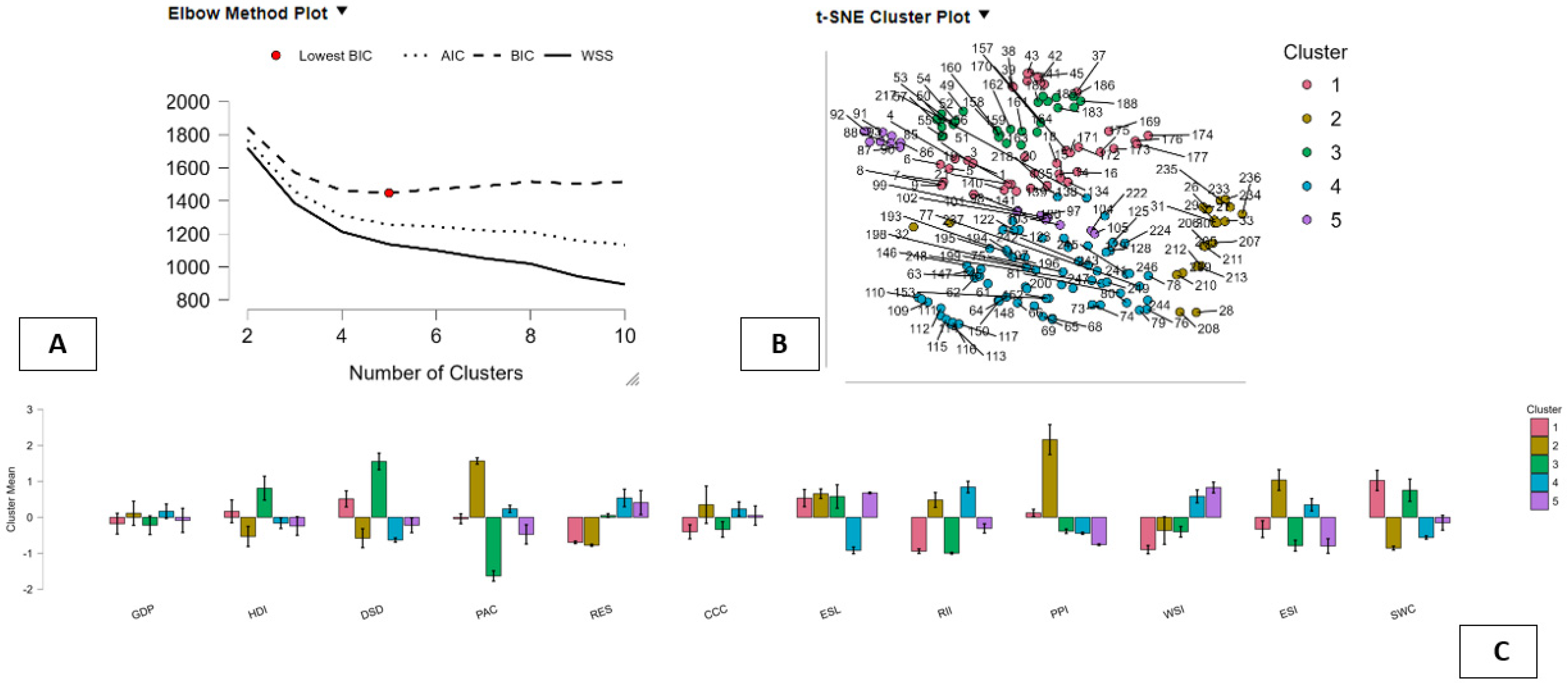
The clustering results identify five distinct territorial profiles, highlighting substantial heterogeneity in the relationship between sustainability and regional GDP in Italy. These profiles show that sustainability-related conditions are not associated with economic performance in a uniform way, but rather differ according to the interaction between environmental quality, innovation, services, and territorial characteristics [123,124]. Some clusters combine positive economic performance with strong environmental and institutional conditions, while others show weak or even negative associations between sustainability and growth. In particular, sustainability alone does not guarantee higher GDP, as positive economic outcomes emerge primarily where environmental factors are combined with innovation capacity and institutional support. Other clusters exhibit mismatches between economic performance and social or environmental conditions, reflecting uneven development patterns. Overall, the findings suggest that the relationship between sustainability and economic growth is complex and conditional, depending on the interaction between environmental, social, and institutional factors. These results are consistent with recent literature on regional development and sustainability transitions [125,126,127]. See

Table 11. Random Forest Clusters of S–Sustainability and Regional GDP Profiles.

Cluster	GDP	HDI	DSD	PAC	RES	CCC	ESL	RII	PPI	WSI	ESI	SWC
1	−0.17	0.16	0.51	−0.04	−0.69	−0.40	0.53	−0.94	0.12	−0.89	−0.32	1.02
2	0.11	−0.53	−0.58	1.56	−0.77	0.35	0.65	0.48	2.16	−0.36	1.03	−0.85
3	−0.21	0.81	1.55	−1.63	0.05	−0.337	0.57	−0.99	−0.38	−0.40	−0.78	0.75
4	0.17	−0.16	−0.63	0.23	0.53	0.23	−0.91	0.84	−0.44	0.58	0.34	−0.56
5	−0.08	−0.24	−0.22	−0.47	0.41	0.05	0.67	−0.30	−0.76	0.83	−0.79	−0.15

Note. This table reports standardized cluster means for GDP and BES S–Sustainability indicators derived from Random Forest clustering. Positive values indicate above-average performance. The clusters reveal distinct territorial models linking environmental quality, energy transition, service reliability, innovation, digital skills, and economic outcomes across Italian regions.

.

The Random Forest results identify a limited set of key determinants of regional GDP within the S–Sustainability dimension. Innovation capacity (PPI) emerges as the most important factor, followed by water service reliability (WSI) and environmental satisfaction (ESL). Renewable energy (RES) and research and innovation intensity (RII) also contribute, while other variables play a marginal role. These findings suggest that economic performance is primarily driven by the interaction between innovation, service reliability, environmental quality, renewable energy, and research intensity. Overall, sustainability appears as a structural component of regional development rather than a secondary outcome, in line with recent literature [128,129,130]. See

Table 12. Boosting Feature Importance of BES Sustainability Indicators for Regional GDP.

Feature	RES	ESL	PAC	PPI	SWC	WSI	DSD	RII	HDI	CCC	ESI
Relative Influence (×103)	327.0	297.0	250.0	8.1	1.4	1.2	1.1	1.0	0.0	0.0	0.0
Mean Dropout Loss (×1011)	0.74	0.69	8.00	6.25	5.98	5.98	5.98	6.00	5.98	5.98	5.98

Note. This table reports boosting-based feature importance using relative influence and permutation dropout loss. Higher values indicate a stronger contribution to GDP prediction. The results show that renewable energy, environmental satisfaction, and protected areas are the main sustainability drivers.

.

The BES S-component used in the Random Forest model groups indicators into broad domains: environmental quality, climate stress, energy transition, innovation, digital skills, and service reliability. These variables capture both environmental conditions and structural characteristics across regions. Rather than detailing each indicator, the model exploits their joint variation to assess how sustainability dimensions interact in explaining regional GDP. This integrated approach is consistent with recent work on sustainable development and regional economic performance [131,132,133]. See Figure 8.

7. Well-Being, Equity and Sustainability as Engines of Regional Growth

The results support the BES framework as a useful approach for interpreting regional economic performance from a multidimensional perspective. By combining panel econometrics, machine learning, and clustering, the analysis highlights the role of well-being within complex social, institutional, environmental, and territorial systems. In particular, the Benessere dimension shows that security, healthcare, mobility, digital access, and social participation are associated with GDP. The Equità dimension indicates that economic growth may coexist with income disparities, poverty risk, healthcare pressure, labour-market exclusion, and difficulties in accessing essential services. The Sostenibilità dimension shows that environmental quality, climate stress, energy transition, innovation, digital skills, and service reliability interact with GDP in a conditional and context-specific manner. Overall, the findings suggest that well-being, equity, and sustainability are key components of regional economic performance rather than simple outcomes of growth [131,132,134]. See

Table 13. Summary of Empirical Evidence on BES Dimensions and Regional GDP in Italy.

Dimension	Indicator/Method	Main Result	Economic Interpretation	Policy Implication
B—Well-being	Crime (FE)	Negative effect on GDP	Insecurity discourages investment	Strengthen public safety
	Public Transport (FE, RF)	Positive effect	Mobility increases productivity	Invest in transport
	Medical Doctors (FE, RF)	Positive effect	Health improves productivity	Expand healthcare
	Digital Access (RF)	Key predictor	Connectivity supports innovation	Reduce the digital divide
E—Equity	Disposable Income (FE, Boosting)	Strong positive effect	Demand drives growth	Support household income
	Poverty Risk (Boosting)	High importance	Vulnerability weakens growth	Reduce poverty
	NEET, Service Access (FE)	Mixed/positive link	Growth may coexist with exclusion	Promote inclusive policies
S—Sustainability	Environmental Factors (RF, Boosting)	Relevant for clusters	Sustainability shapes growth patterns	Integrate green policies
Territorial Structure	Clustering	Distinct regimes	Regions follow different paths	Place-based policies
Nonlinearity	KNN, RF	Best performance	Growth is nonlinear and local	Avoid one-size-fits-all
Systemic Interaction	Combined BES	Multidimensional effect	Growth is systemic	Coordinate policies

Note. This table synthesizes results from panel regressions, machine learning, and clustering. It shows how BES dimensions—well-being, equity, and sustainability—jointly shape regional GDP through security, health, income, infrastructure, and environmental quality, supporting a multidimensional model of economic development.

.

8. Building GDP Through Social, Institutional and Environmental Capital

The results have clear implications for Italian economic policy, suggesting a shift from a purely growth-centered approach toward a multidimensional strategy based on the BES framework. Economic performance depends not only on traditional factors but also on social, institutional, and environmental conditions. Public spending on security and infrastructure should be considered a productive investment, as lower crime and better transport systems are associated with higher GDP. Similarly, healthcare emerges as a key driver of economic performance, supporting the view that health constitutes productive capital, particularly in lagging regions. The findings also highlight the importance of equity, as growth may coexist with social imbalances, indicating the need for more inclusive development strategies. Finally, environmental quality and green investments play a relevant role in sustaining long-term competitiveness [135,136].

9. Discussion of the Results

From an empirical perspective, the results provide a sound interpretation of the relationship between multidimensional well-being and regional economic performance in Italy. Overall, the findings show that GDP is not determined solely by conventional economic determinants but also by social, institutional, environmental, and territorial factors. Thus, the key thesis of this paper is supported: the BES approach can help explain the relationship between well-being, equity, sustainability, and regional economic development [63,64]. Starting with the Benessere dimension, panel data estimations reveal negative associations between crime indicators and GDP, and positive associations between Public Transport Supply and Medical Doctors Density and GDP. These findings show that safety, mobility, and healthcare access are not merely social indicators, but productive factors of local economies. Lower crime rates may boost trust, reduce transaction costs, and make localities more attractive for investment and businesses. Public transport supports accessibility, workforce mobility, and integration into wider markets, while healthcare access contributes to human capital, labour productivity, and regional resilience [137,138]. The use of machine learning tools also supports this thesis. The KNN model shows that Public Transport Supply is the most important predictor of regional GDP, followed by variables related to security and healthcare. This result indicates that the relationship between well-being and GDP is nonlinear and depends on the local configuration of infrastructures, services, and social conditions. This is consistent with current research using machine learning tools for well-being analysis in Italy [67,139]. Clustering analysis further confirms the existence of different territorial regimes, distinguishing regions with high GDP and strong Benessere performance from those with lower GDP and weaker well-being conditions. Second, the findings for the Equità dimension show that GDP is positively associated with Gross Disposable Income per Capita. This indicates that household income, purchasing power, and demand influence regional economic performance. At the same time, the positive association of GDP with youth exclusion and service access difficulty should be interpreted critically. These results do not imply that exclusion or limited access to services improve economic performance. Rather, they suggest that economic growth may coexist with social imbalances. Boosting models confirm this interpretation by showing that General Practitioners Overload, disposable income, and poverty risk are among the most relevant predictors of GDP. This means that healthcare pressure, income conditions, and poverty dynamics are key channels through which equity interacts with regional economic performance, in line with the literature on multidimensional poverty [140,141]. Clustering analysis confirms clear territorial differences between economically stronger regions and areas characterized by poverty risk, labour-market non-participation, youth exclusion, severe material and social deprivation, healthcare overload, and difficulty accessing essential services. Finally, concerning the Sostenibilità dimension, the results show positive associations between GDP and sustainability indicators such as Heatwave Duration Index, Climate Change Concern, and Biodiversity Loss Concern. These associations should not be interpreted causally, but structurally. More developed regions may be more exposed to environmental pressures and may also display higher environmental awareness. In this sense, sustainability becomes an endogenous characteristic of the development process, where environmental stress and awareness evolve together. This is confirmed by previous findings on SDG interlinkages [142,143]. Machine learning models further show that Renewable Energy Share, Environmental Satisfaction Level, and Protected Area Coverage are key predictors of GDP within the Sostenibilità dimension. SHAP analysis suggests that some sustainability variables may generate short-term trade-offs with GDP growth, as they require adjustments in local economies. However, such trade-offs do not exclude the long-term role of sustainability as a precondition for regional development, implying that energy transition and environmental protection should be complemented by investment in innovation, digital skills, service reliability, institutions, and territorial planning. In conclusion, the BES dimensions affect GDP growth in different but complementary ways: Benessere acts mainly through security, mobility, healthcare, digital access, and social participation; Equità acts through income, poverty risk, healthcare pressure, labour-market participation, youth exclusion, deprivation, and access to services; Sostenibilità acts through environmental quality, climate stress, renewable energy, protected areas, innovation, digital skills, and service reliability. The main contribution of this study is to show that the three dimensions need to be combined in the analysis. Regional economic performance is shaped by their joint action. The combination of econometrics, machine learning, and clustering makes this interpretation possible: econometric models detect statistically significant associations; machine learning tools identify nonlinear relationships and predictor importance; and clustering analysis highlights territorial heterogeneity and differentiated development regimes. From a theoretical perspective, the empirical results support the hypothesis that well-being, equity, and sustainability are not merely consequences of economic growth, but preconditions that shape the capacity of territories to generate economic performance. This conclusion is particularly relevant given the pronounced regional disparities in Italy [143]. Therefore, since the BES–GDP relationship is complex and territorially heterogeneous, place-based policies are needed, and the BES framework can serve as a basis for regional policy design [63].

10. Policy Implications for Integrated and Inclusive Regional Development

The results have important implications for Italian economic policy. They show that well-being, equity, and sustainability are structural drivers of regional economic performance rather than outcomes of growth. Accordingly, policies traditionally viewed as “social” or “environmental” should be treated as core components of growth strategies.

Investments in security, healthcare, and transport infrastructure are directly associated with higher economic performance. At the same time, income distribution, poverty, and access to services shape growth dynamics, indicating that development accompanied by social imbalances is unlikely to be sustainable. Environmental quality, energy transition, and innovation also contribute to competitiveness, despite potential short-term trade-offs.

The marked territorial heterogeneity across regions implies that uniform policies are ineffective. A place-based, multidimensional approach—consistent with the BES framework—is required to address diverse regional conditions [144,145].

These findings also highlight the role of decentralization and local governance. Effective policy design depends on adapting interventions to local contexts, supported by adequate institutional capacity and investment in social and environmental infrastructure. Without these conditions, territorial disparities are likely to persist.

The current paper provides a strong rationale for the adoption of a decentralization-focused policy approach for Italy. The consistent presence of territory heterogeneity through the findings of panel regressions, machine-learning algorithms, and cluster analysis clearly indicates that there are no similarities between the development paths of Italian regions. They vary based on their unique socio-economic, institutional, and environmental configurations and exhibit different degrees of prosperity, equity, and sustainability. Therefore, centralized and standardized policies are not only insufficient in this situation but may even be counterproductive as they ignore regional diversity [146,147]. This highlights the importance of a place-based decentralization model under which regions would assume responsibility for designing regional economic policies. According to the Benessere findings, several major determinants of economic success are institutionally and territorially tied. As such, decentralized governance should not be considered an intermediate step but a basic determinant of a region’s economic achievements [148,149]. In addition, the Equità findings suggest that regional inequality cannot be adequately addressed if it is not taken into consideration during policy-making and intervention. Economic success does not guarantee that a region will not face issues related to persistent and geographically clustered inequality. To solve this problem, local and regional efforts will have to be made to ensure access to opportunities and reduce disparities [148,150]. The non-linear relationships detected via machine-learning techniques also support the proposed approach. The socio-economic and environmental characteristics affect GDP depending on region-specific configurations of factors. Thus, there are no generalized policy approaches that work equally well in all regions of Italy [147]. At the same time, this study demonstrates that decentralization per se is not enough to achieve regional balance. The efficiency of such policies is directly determined by their implementation in a particular region with its own socio-economic and institutional configuration. Under unfavorable conditions, decentralization could further enhance differences due to stronger regions’ ability to capitalize on their strengths in comparison to weaker neighbors [147,150]. Hence, it is evident that decentralized governance has to be accompanied by strengthening institutional capacities and building multilevel cooperation between the involved stakeholders [150]. Overall, the above findings allow for positioning decentralization as a crucial element of any successful development strategy. Through the application of the BES model together with the obtained evidence, it became clear that economic performance is inseparably associated with territorial and place-based social, institutional, and environmental characteristics. As a result, decentralized policy design could be viewed as a necessary precondition for efficient economic and social outcomes [147,149].

11. Conclusions

Conclusively, the research shows that well-being, equity, and sustainability should not be seen merely as consequences of economic growth, but as structural conditions shaping regional economic performance. Differences in security, healthcare access, mobility, income, poverty risk, service accessibility, environmental quality, energy transition, innovation, digital skills, and service reliability drive heterogeneous development trajectories across Italian regions. This confirms the importance of a multidimensional approach to development. From a policy perspective, the findings suggest that measures focused on improving security, healthcare, mobility, inclusion, environmental quality, renewable energy, innovation, and essential services may support regional productivity and growth. Given territorial disparities in Italy, uniform policy actions cannot fully address regional development challenges. The main contribution of the study lies in providing new empirical evidence through an integrated framework combining panel econometrics, machine learning, and clustering analysis. At the same time, the findings should not be interpreted as definitive causal evidence.

References

1. Stiglitz, J.E.; Sen, A.; Fitoussi, J.P. Mismeasuring Our Lives: Why GDP Doesn’t Add Up; The New Press: New York, NY, USA, 2010. [Google Scholar]
2. Kroll, C.; Warchold, A.; Pradhan, P. Sustainable Development Goals (SDGs): Are we successful in turning trade-offs into synergies? Palgrave Commun. 2019, 5, 140. [Google Scholar] [CrossRef]
3. Durand, M.; Exton, C. Adopting a well-being approach in central government: Policy mechanisms and practical tools. In Global Happiness and Wellbeing; University of Oxford’s Wellbeing Research Centre: Oxford, UK, 2019. [Google Scholar]
4. Decancq, K.; Schokkaert, E. Beyond GDP: Using equivalent incomes to measure well-being in Europe. Soc. Indic. Res. 2016, 126, 21–55. [Google Scholar] [CrossRef]
5. Tenaglia, S. Gli indicatori di benessere nella programmazione economica in Italia. Un esempio virtuoso di sinergia tra ricerca e policy making. Sinappsi 2022, XII, 14–25. [Google Scholar] [CrossRef]
6. Ahammed, S.; Rana, M.M.; Uddin, H.; Majumder, S.C.; Shaha, S. Impact of blue economy factors on the sustainable economic growth of China. Environ. Dev. Sustain. 2025, 27, 12625–12652. [Google Scholar] [CrossRef]
7. Berberoglu, Y.; Mangla, S.K.; Kazancoglu, Y. Towards sustainable mining in an emerging economy: Assessment of sustainability challenges. Resour. Policy 2024, 97, 105288. [Google Scholar] [CrossRef]
8. Chengliang, Y.; Fuyang, Z.; Huan, N. Environmental target responsibility system, governance, and economic growth. China Econ. 2025, 20, 2–27. [Google Scholar]
9. Gylfason, T.; Nganou, J.-P.N. Balancing natural resources and human and social capital: Pathways to economic diversification in Mongolia. Comp. Econ. Stud. 2025, 67, 289–325. [Google Scholar] [CrossRef]
10. Haroon, M.; Hayyat, M. Assessing the dual impact of gold mining on local communities: Socio-economic benefits and environmental challenges. Resour. Policy 2025, 103, 105559. [Google Scholar] [CrossRef]
11. Hwang, Y.K.; Díez, Á.S.; Inglesi-Lotz, R. The effects of critical mineral endowments on green economic growth in Latin America. Resour. Policy 2024, 98, 105355. [Google Scholar] [CrossRef]
12. Infante-Amate, J.; Travieso, E.; Aguilera, E. Unsustainable prosperity? Decoupling wellbeing, economic growth, and greenhouse gas emissions over the past 150 years. World Dev. 2024, 184, 106754. [Google Scholar] [CrossRef]
13. Le, H.C.; Bhattacharya, M.; Smyth, R.; Zhang, X. Does economic growth cause energy intensity of well-being in the very long run? Semi-parametric evidence for selected OECD countries. Energy Econ. 2024, 139, 107889. [Google Scholar] [CrossRef]
14. Zéman, Z.; Kálmán, B.G.; Vasa, L. The impact of domestic material consumption and energy mix on socioeconomic indicators: A global analysis from 1990 to 2022. Resour. Policy 2025, 107, 105658. [Google Scholar] [CrossRef]
15. Du, J.; Gu, H.; Shen, Z.; Song, M.; Vardanyan, M. Assessing regional energy security characteristics: Evidence from Chinese province-level data. Energy Econ. 2024, 140, 107964. [Google Scholar] [CrossRef]
16. Insaidoo, M.; Kunawotor, M.E.; Ahiabor, G. Extreme weather events and economic growth: Empirical evidence from Africa. Afr. J. Econ. Manag. Stud. 2025. ahead-of-print. [Google Scholar] [CrossRef]
17. Anauati, M.V.; Gómez Seeber, M.; Campanario, S.; Sosa-Escudero, W.; Golombek, D.A. The economic costs and consequences of (insufficient) sleep: A case study from Latin America. Eur. J. Health Econ. 2025, 26, 711–719. [Google Scholar] [CrossRef] [PubMed]
18. Barbier, E.B.; Mensah, A.C.E. Environmental health risks, welfare and GDP. J. Environ. Econ. Manag. 2025, 133, 103206. [Google Scholar] [CrossRef]
19. Dar, K.H.; Raina, S.H.; Sajjad, S.; Showkat, M. Does environment and health impact economic growth in presence of asymmetries? Evidence from G7 economies using panel nonlinear ARDL. J. Econ. Adm. Sci. 2025. ahead-of-print. [Google Scholar] [CrossRef]
20. Hussien, H.H.; Hagabdulla, N.H.; Ahmed, K.M.Y.; Albadwi, F.I.A.; Alotaibi, K.N. The impact of economic growth on public health and well-being: An empirical analysis of Saudi Arabia. J. Open Innov. Technol. Mark. Complex. 2025, 2, 100564. [Google Scholar] [CrossRef]
21. Iuga, I.C.; Nerișanu, R.A.; Iuga, H. How a nation’s well-being influences its health profile: An analysis of critical indicators. Eur. J. Health Econ. 2025, 26, 1439–1457. [Google Scholar] [CrossRef]
22. Islam, M.S.; Baida, U. Determinants of health expenditure in GCC countries: Exploring environmental quality, economic growth and education dynamics. Millenn. Asia 2025. [Google Scholar] [CrossRef]
23. Akinlo, A.E.; Okunlola, C.O. The effect of economic freedom on quality of life: Exploring the role of political risk factors in Africa. J. Interdiscip. Econ. 2025, 37, 42–68. [Google Scholar] [CrossRef]
24. Kunawotor, M.; Ahiabor, G.; Yobo, E. Government size, institutional quality and economic welfare in Africa. Int. J. Soc. Econ. 2025, 52, 578–590. [Google Scholar] [CrossRef]
25. Martynenko, V.; Korzh, M.; Sokolova, O.; Koliada, T.; Jadallah, O. Comprehensive assessment of the impact of financial decentralization on the sustainable development of Ukraine’s regions in the context of implementing European experience. Financ. Credit Act. Probl. Theory Pract. 2025, 4, 330–342. [Google Scholar]
26. Grashof, N. Rethinking regional performance: Examining the role of economic growth and industrial clusters in the objective well-being of European regions. Rev. Reg. Res. 2025, 45, 421–464. [Google Scholar] [CrossRef]
27. Crozet, M.; Hering, L.; Poncet, S. Is there a bright side to the China syndrome? Rising export opportunities and life satisfaction in China. World Bank Econ. Rev. 2024, 38, 708–740. [Google Scholar] [CrossRef]
28. Buscemi, T. From the little divergence to the little divide: Real wages in the Kingdom of Sicily (1540–1850). Econ. Hist. Rev. 2025, 78, 646–672. [Google Scholar] [CrossRef]
29. Chakori, S.; Grigg, N.J.; Biely, K.; Richards, R.; Robra, B. From innovation to exnovation: Insights from post-growth food enterprises in Australia. Ecol. Econ. 2026, 239, 108785. [Google Scholar] [CrossRef]
30. Lauer, A.; Capellán-Pérez, I.; Wergles, N. A comparative review of de- and post-growth modeling studies. Ecol. Econ. 2025, 227, 108383. [Google Scholar] [CrossRef]
31. Levy, N. Economic policy of the first government of the 4T: Future directions. Cuad. Econ. 2025, 44, 237–261. [Google Scholar]
32. Mažeikaitė, K. Assessing the causal impact of culture on socio-economic variables in European countries. J. Interdiscip. Econ. 2025, 37, 200–219. [Google Scholar] [CrossRef]
33. Tleuberdinova, A.T.; Panzabekova, A.Z.; Khalitova, M.M.; Suleimenova, A.S. Population engagement in contemporary economic issues of the country: Interregional comparison. Econ. Strategy Pract. 2025, 20, 123–138. [Google Scholar] [CrossRef]
34. Mikheeva, N.N. Priority geostrategic regions of spatial development strategies for Russia. Reg. Res. Russ. 2025, 15, 589–597. [Google Scholar] [CrossRef]
35. Tan, Y.-T.; Gan, P.-T.; Hadi, F.S.A.; Gamal, A.A.M. Tourism’s impact on economic and human development: Evidence from ASEAN-5. Econ. Reg. 2025, 21, 166–179. [Google Scholar] [CrossRef]
36. Utouh, H.M.L.; Kitole, F.A. Opportunity cost of mega infrastructure projects in Africa: Should development be traded for growth? Evidence from Tanzania. Cogent Econ. Financ. 2025, 13, 2524572. [Google Scholar] [CrossRef]
37. Mohamed, A.A.; Mohamed, S.N.; Weyrah, I.M.; Isse, M.D.; Husein, I.A. Determinants of economic well-being and human development in Somalia: A dual analysis of GDP per capita and life expectancy. Cogent Econ. Financ. 2025, 13, 251348. [Google Scholar] [CrossRef]
38. Munawaroh, T.; Sukamdi, R.A.; Listyaningsih, U. The macroeconomic impact of population aging in Indonesia: Do older adults matter? Asian Econ. Financ. Rev. 2025, 15, 383–403. [Google Scholar] [CrossRef]
39. Warner, M.E.; Zhang, X.; Guillemot, J. Demographic ageing: An opportunity to rethink economy, society and regions. Camb. J. Reg. Econ. Soc. 2025, 18, 79–92. [Google Scholar] [CrossRef]
40. Zhou, J.; Song, J.; Huang, X. Human capital, well-being and growth rate of rural–urban migration in China. Singap. Econ. Rev. 2025, 70, 1159–1192. [Google Scholar] [CrossRef]
41. Natanael, Y. Is less commodity dependence better for economic equality, economic growth, and human development? Glob. J. Emerg. Mark. Econ. 2025, 17, 199–221. [Google Scholar] [CrossRef]
42. Okogun, O.; Hiwatari, M. Multidimensional poverty analysis of women, children and households in Nigeria: The first order dominance approach. Afr. J. Econ. Manag. Stud. 2024, 15, 602–619. [Google Scholar] [CrossRef]
43. Rijpma, A.; Philips, R.C.M.; van Bavel, B.J.P. Multidimensional composite indicators of well-being: Applications in economic history. J. Econ. Surv. 2025, 39, 672–705. [Google Scholar] [CrossRef]
44. Yeboah, S.D.; Gatsi, J.G.; Appiah, M.O.; Fumey, M.P. Examining the drivers of inclusive growth: A study of economic performance, environmental sustainability, and life expectancy in BRICS economies. Res. Glob. 2024, 9, 100267. [Google Scholar] [CrossRef]
45. Lobonț, O.-R.; Criste, C.; Bovary, C.; Țăran, A.-M. Settling the debate: Does digitalisation impact the economic growth in the European Union member states? Technol. Econ. Dev. Econ. 2025, 31, 980–1007. [Google Scholar] [CrossRef]
46. Mashaqbeh, H.M.D. The impact of remittances on household consumption and economic growth in Jordan. Int. J. Account. Econ. Stud. 2025, 12, 266–274. [Google Scholar] [CrossRef]
47. Tian, T.; Nie, B.; Zhang, X.; Li, X.; Hong, X. Analyzing the socially sustainable impacts of private investments in the mining sector in rural areas. Resour. Policy 2024, 98, 105347. [Google Scholar] [CrossRef]
48. Tiwari, S.; Cheong, C.W.H.; See Mey, L.; Saji, T.G. Does fintech really matter for energy, economy and environment? From the lenses of SDG-7, SDG-8, SDG-13, COP27 and COP28. Resour. Policy 2024, 98, 105318. [Google Scholar] [CrossRef]
49. Wu, S.; Michailova, S.; Fan, D. Legitimacy under pressure: Energy firms’ expansion in countries with weak environmental performance. World Dev. 2025, 185, 106800. [Google Scholar] [CrossRef]
50. Kopczewska, K. Spatial machine learning: New opportunities for regional science. Ann. Reg. Sci. 2022, 68, 713–755. [Google Scholar] [CrossRef]
51. Westerholt, R. Exploratory statistical analysis of spatial structures in urban datasets. In Metropolitan Research: Methods and Approaches; Transcript Verlag: Bielefeld, Germany, 2022; pp. 37–61. [Google Scholar]
52. Wu, H. Statistics evolution and revolution to meet data science challenges. Stat. Biosci. 2025, 17, 813–831. [Google Scholar] [CrossRef]
53. Giannone, D.; Lenza, M.; Primiceri, G.E. Economic predictions with big data: The illusion of sparsity. Econometrica 2021, 89, 2409–2437. [Google Scholar] [CrossRef]
54. Mullainathan, S.; Spiess, J. Machine learning: An applied econometric approach. J. Econ. Perspect. 2017, 31, 87–106. [Google Scholar] [CrossRef]
55. Varian, H. Artificial intelligence, economics, and industrial organization. In The economics of Artificial Intelligence: An Agenda; University of Chicago Press: Chicago, IL, USA, 2018; pp. 399–419. [Google Scholar]
56. Chernozhukov, V.; Demirer, M.; Duflo, E.; Fernandez-Val, I. Generic machine learning inference on heterogeneous treatment effects in randomized experiments, with an application to immunization in India. Natl. Bur. Econ. Res. 2018, 93, w24678. [Google Scholar]
57. Drago, C.; Costantiello, A.; Arnone, M.; Anobile, F.; Leogrande, A. Mapping the association between energy use and ESG dimensions: Evidence from panel econometrics, clustering, and machine learning. Energies 2026, 19, 828. [Google Scholar] [CrossRef]
58. Capello, R.; Caragliu, A. Digital transition in a turbulent world: European regional growth opportunities in 17 years’ time. Econ. Innov. New Technol. 2025, 34, 997–1015. [Google Scholar] [CrossRef]
59. Dellisanti, R. Cultural and creative industries and local economic growth: Exploring the urban channel. Spat. Econ. Anal. 2025, 20, 457–483. [Google Scholar] [CrossRef]
60. Bonaccorsi, G.; Scotti, F.; Flori, A.; Pammolli, F. Balancing health and economic impacts from targeted pandemic restrictions. J. Evol. Econ. 2023, 33, 1047–1083. [Google Scholar] [CrossRef]
61. Brandano, M.G.; Faggian, A.; Pinate, A.C. The impact of COVID-19 on the tourism sector in Italy: A regional spatial perspective. Tour. Econ. 2024, 30, 2181–2202. [Google Scholar] [CrossRef]
62. Gallo, G.; Granato, S.; Raitano, M. Covid-19 heterogeneous effects on Italian workers’ incomes: The role of jobs routinization and teleworkability. Int. J. Manpow. 2024, 45, 1326–1349. [Google Scholar] [CrossRef]
63. Bacchini, F.; Baldazzi, B.; De Carli, R.; Di Biagio, L.; Savioli, M.; Sorvillo, M.P.; Tinto, A. The evolution of the Italian framework to measure well-being. J. Off. Stat. 2021, 37, 317–339. [Google Scholar] [CrossRef]
64. Onori, F.; Lasinio, G.J. Modeling “Equitable and Sustainable Well-being” (BES) Using Bayesian Networks. Soc. Indic. Res. 2022, 161, 1003–1037. [Google Scholar] [CrossRef]
65. Magazzino, C.; Costantiello, A.; Laureti, L.; Leogrande, A.; Gattone, T. Greenhouse gas emissions and road infrastructure in Europe: A machine learning analysis. Transp. Res. Part D 2025, 139, 104602. [Google Scholar] [CrossRef]
66. Levantesi, S.; Nigri, A.; Pagnottoni, P.; Spelta, A. Wasserstein barycenter regression: Application to the joint dynamics of regional GDP and life expectancy in Italy. ASTA Adv. Stat. Anal. 2025, 109, 313–336. [Google Scholar] [CrossRef]
67. Firza, N.; Antonucci, L.; Crocetta, C.; d’Ovidio, F.D.; Monaco, A. Spatial analysis to investigate the relationship between tourism and wellbeing in Italy. Soc. Indic. Res. 2024, 175, 1027–1043. [Google Scholar] [CrossRef]
68. Sharma, V.; Mahajan, Y.; Kapse, M. Exploring subjective well-being using machine learning: GDP, health, social support, and emotional factors. Cogent Soc. Sci. 2025, 11, 2569758. [Google Scholar] [CrossRef]
69. Huanco Ramos, F.; Valentin Ccori, Y.; Shuta Lloclla, H.; Yucra Sotomayor, M.; Mamani Uchasara, I. Economic Growth and Fiscal Policy in Peru: Prediction Using Machine Learning Models. Int. J. Adv. Comput. Sci. Appl. 2025, 16, 41. [Google Scholar] [CrossRef]
70. Samartzidis, L.; Quatrosi, M.; von Dulong, A. Gender and Age Matter! Identifying Important Predictors for Subjective Well-being Using Machine Learning Methods. Soc. Indic. Res. 2025, 179, 955–978. [Google Scholar] [CrossRef]
71. Navarro-Acosta, J.A.; Soto-Mendoza, V.; Policardo, L.; Sánchez-Carrera, E.J. Modeling economic growth in pandemic times with machine learning regression algorithms. Rev. Mex. Econ. Finanz. 2025, 20, 8. [Google Scholar] [CrossRef]
72. Miconi, F.; Dimitri, G.M. A machine learning approach to analyse and predict the electric cars scenario: The Italian case. PLoS ONE 2023, 18, e0279040. [Google Scholar] [CrossRef]
73. Suleiman, H.; Nguyen, M.T.T.; Mendez, C. Predicting subnational GDP in Vietnam with remote sensing data: A machine learning approach. Lett. Spat. Resour. Sci. 2025, 18, 5. [Google Scholar] [CrossRef]
74. Xu, T.; Zong, Y.; Su, H.; Tian, A.; Gao, J.; Wang, Y.; Su, R. Prediction of multi-scale socioeconomic parameters from long-term nighttime lights satellite data using decision tree regression: A case study of Chongqing, China. Land 2023, 12, 249. [Google Scholar] [CrossRef]
75. Avcı Azkeskin, S.; Aladağ, Z. Evaluating regional sustainable energy potential through hierarchical clustering and machine learning. Environ. Res. Commun. 2025, 7, 015002. [Google Scholar] [CrossRef]
76. Desita, R.K.; Fahmi, A.; Rohmani, A.; Sulistyono, M.T. Agglomerative Hierarchical Clustering For Regional Grouping In Central Java Based On Welfare Indices. J. Pilar Nusa Mandiri 2025, 21, 108–116. [Google Scholar] [CrossRef]
77. Musa, M.; Fallo, S.I. Hierarchical cluster analysis on people’s welfare in southeast sulawesi province. BAREKENG J. Ilmu Mat. Dan Terap. 2023, 17, 1163–1172. [Google Scholar] [CrossRef]
78. Gusmanov, R.; Stovba, E.; Kuznetsova, A.; Gusmanov, I.; Taipov, T.; Muhametshina, G.; Akhmetova, L. Rural area sustainable development strategies on the basis of a cluster approach. Reg. Sci. Policy Pract. 2022, 14, 778–796. [Google Scholar] [CrossRef]
79. Kostakis, I.; Tsagarakis, K.P. The role of entrepreneurship, innovation and socioeconomic development on circularity rate: Empirical evidence from selected European countries. J. Clean. Prod. 2022, 348, 131267. [Google Scholar] [CrossRef]
80. Rahma, N.Z.C.; Rustiadi, E.; Pravitasari, A.E. Enhancing Urban and Peri-Urban Zoning Using Spatially Constrained Clustering: Evidence from the Jakarta–Bandung Mega-Urban Region. Land 2026, 15, 534. [Google Scholar] [CrossRef]
81. Indah, Y.M.; Kuswandi, W. Clustering Analysis for Regional Variations in Beef Production: A Comparative Study of Hierarchical and Non-Hierarchical. Statistika 2025, 25, 43–49. [Google Scholar] [CrossRef]
82. Nuralifian, M.Z.; Nooraeni, R. Grouping Provinces in Indonesia Based on Youth Development Indicators in 2021. J-3P (J. Pembang. Pemberdaya. Pemerintah.) 2023, 8, 1–18. [Google Scholar] [CrossRef]
83. Eminov, Z.N.; Imrani, Z.T.; Gasimova, E.E.; Vysotskyi, O.Y. Possibilities of applying the cluster approach in the study of the stability of the regional territorial organisation of production areas. J. Geol. Geogr. Geoecol. 2024, 33, 54–62. [Google Scholar] [CrossRef]
84. Strelchenko, I.; Koczar, J.; Pysarkova, V. Using cluster analysis to assess financial stability as an object of managerial impact of regional competitive immunity. Acad. Rev. 2022, 2, 111–124. [Google Scholar] [CrossRef]
85. Karma, E. NEET youth in central and eastern European countries: A panel model approach. J. Youth Stud. 2025, 28, 1458–1475. [Google Scholar] [CrossRef]
86. Amendola, S. Macro-determinants of neet: An ecological study at the country level of analysis for the period 1997–2020. Youth 2022, 2, 384–390. [Google Scholar] [CrossRef]
87. Komatsu, S.; Suzuki, A. The impact of different levels of income inequality on subjective well-being in China: A panel data analysis. Chin. Econ. 2023, 56, 104–123. [Google Scholar] [CrossRef]
88. Basumatary, I.R.; Das, M.; Basumatary, S.; Basumatary, K. Macroeconomic determinants of income inequality among different income group countries: Evidence from panel data. J. Soc. Econ. Res. 2024, 11, 111–125. [Google Scholar] [CrossRef]
89. Akarsu, G. Spatial panel data analysis of the relationship between tourism and income inequality. Anatolia 2022, 33, 537–549. [Google Scholar] [CrossRef]
90. Das, P.K.; Das, P.K. Forecasting and analyzing predictors of inflation rate: Using machine learning approach. J. Quant. Econ. 2024, 22, 493–517. [Google Scholar] [CrossRef]
91. Babii, A.; Ghysels, E.S.J. Econometrics of machine learning methods in economic forecasting. In Handbook of Research Methods and Applications in Macroeconomic Forecasting; Edward Elgar Publishing: Cheltenham, UK, 2024; pp. 246–273. [Google Scholar]
92. Lechner, M. Causal Machine Learning and its use for public policy. Swiss J. Econ. Stat. 2023, 159, 8. [Google Scholar] [CrossRef]
93. Adler, A.I.; Painsky, A. Feature importance in gradient boosting trees with cross-validation feature selection. Entropy 2022, 24, 687. [Google Scholar] [CrossRef]
94. Touati, S.; Benghia, A.; Hebboul, Z.; Lefkaier, I.K.; Kanoun, M.B.; Goumri-Said, S. Predictive machine learning approaches for perovskites properties using their chemical formula: Towards the discovery of stable solar cells materials. Neural Comput. Appl. 2024, 36, 16319–16329. [Google Scholar] [CrossRef]
95. Pérez-Sánchez, I.; Medina-Pérez, M.A.; Monroy, R.; Loyola-González, O.; Gutierrez-Rodríguez, A.E. New evaluation method for fuzzy cluster validity indices. IEEE Access 2025, 13, 22728–22744. [Google Scholar] [CrossRef]
96. Chugh, D.; Mittal, H.; Saxena, A.; Chauhan, R.; Yafi, E.; Prasad, M. Augmentation of densest subgraph finding unsupervised feature selection using shared nearest neighbor clustering. Algorithms 2023, 16, 28. [Google Scholar] [CrossRef]
97. Xue, X.; Lin, J.C.W.; Jiang, Z. Collaborative ontology matching with dual population genetic programming and active meta-learning. IEEE Trans. Evol. Comput. 2025. [Google Scholar] [CrossRef]
98. Crescenzi, R.; Giua, M. The economic impacts of Cohesion Policy. In EU Cohesion Policy; Edward Elgar Publishing: Cheltenham, UK, 2024; pp. 114–124. [Google Scholar]
99. Ejrnæs, A.; Jensen, M.D.; Schraff, D.; Vasilopoulou, S. Introduction: Regional inequality and political discontent in Europe. J. Eur. Public Policy 2024, 31, 1465–1493. [Google Scholar] [CrossRef]
100. Nesari, A.M.; MotieGhader, H.; Ghorbian, S. Advances and challenges in single-cell RNA sequencing data analysis: A comprehensive review. Brief. Bioinform. 2026, 27, bbaf723. [Google Scholar] [CrossRef] [PubMed]
101. Zhou, S.; Xu, H.; Zheng, Z.; Chen, J.; Li, Z.; Bu, J.; Ester, M. A comprehensive survey on deep clustering: Taxonomy, challenges, and future directions. ACM Comput. Surv. 2024, 57, 69. [Google Scholar] [CrossRef]
102. Sagala, N.T.; Gunawan, A.A.S. Discovering the optimal number of crime cluster using elbow, silhouette, gap statistics, and nbclust methods. ComTech Comput. Math. Eng. Appl. 2022, 13, 1–10. [Google Scholar] [CrossRef]
103. Pata, U.K.; Balsalobre-Lorente, D. Exploring the impact of tourism and energy consumption on the load capacity factor in Turkey: A novel dynamic ARDL approach. Environ. Sci. Pollut. Res. 2022, 29, 13491–13503. [Google Scholar] [CrossRef] [PubMed]
104. Murshed, M.; Haseeb, M.; Alam, M.S. The environmental Kuznets curve hypothesis for carbon and ecological footprints in South Asia: The role of renewable energy. GeoJournal 2022, 87, 2345–2372. [Google Scholar] [CrossRef]
105. Triantafyllidou, A.; Polychronidou, P.; Mantzaris, I. Renewable and Non-Renewable Energy Consumption and Economy: A Systematic Literature Review for Greece. Eur. J. Interdiscip. Stud. 2024, 16, 155–174. [Google Scholar] [CrossRef]
106. Ouattara, K.; Gniza, D.I. The Impact of Greenhouse Gas Emissions on GDP per Capita: A Multi-Scale Analysis Using the Wavelet Approach. Int. J. Energy Econ. Policy 2026, 16, 587. [Google Scholar] [CrossRef]
107. Johnstone, I. Organisation for Economic Co-operation and Development (OECD). Yearb. Int. Environ. Law 2023, 34, yvae026. [Google Scholar] [CrossRef]
108. Laureti, L.; Costantiello, A.; Anobile, F.; Leogrande, A.; Magazzino, C. Waste management and innovation: Insights from Europe. Recycling 2024, 9, 82. [Google Scholar] [CrossRef]
109. Magazzino, C.; Madaleno, M.; Waqas, M.; Leogrande, A. Exploring the determinants of methane emissions from a worldwide perspective. Environ. Pollut. 2024, 348, 123807. [Google Scholar] [CrossRef]
110. Madaleno, M.; Nogueira, M.C. How renewable energy and CO2 emissions contribute to economic growth, and sustainability—An extensive analysis. Sustainability 2023, 15, 4089. [Google Scholar] [CrossRef]
111. Leal, P.H.; Marques, A.C. The evolution of the environmental Kuznets curve hypothesis assessment: A literature review under a critical analysis perspective. Heliyon 2022, 8, e11521. [Google Scholar] [CrossRef]
112. Du, J.; Rasool, Y.; Kashif, U. Asymmetric impacts of environmental policy, financial, and trade globalization on ecological footprints: Insights from G9 industrial nations. Sustainability 2025, 17, 1568. [Google Scholar] [CrossRef]
113. Abubakar, I.R.; Alola, A.A.; Bekun, F.V.; Onifade, S.T. Investigating the determinants of household energy consumption in Nigeria: Insights and implications. Energy Sustain. Soc. 2024, 14, 29. [Google Scholar] [CrossRef]
114. Bektaş, V.; Ursavaş, N. Revisiting the environmental Kuznets curve hypothesis with globalization for OECD countries: The role of convergence clubs. Environ. Sci. Pollut. Res. 2023, 30, 47090–47105. [Google Scholar] [CrossRef]
115. Emami, S.; Martínez-Muñoz, G. Condensed-gradient boosting. Int. J. Mach. Learn. Cybern. 2025, 16, 687–701. [Google Scholar] [CrossRef]
116. Manley, W.; Tran, T.; Prusinski, M.; Brisson, D. Modeling tick populations: An ecological test case for gradient boosted trees. Peer Community J. 2023, 3, e116. [Google Scholar] [CrossRef]
117. Sakib, N. Machine Learning-based Travel Time Prediction Models for Complex Traffic Conditions. SSRN 2024, 5238355. [Google Scholar] [CrossRef]
118. Ali, M.; Seraj, M.; Türüç, F.; Tursoy, T.; Raza, A. Do banking sector development, economic growth, and clean energy consumption scale up green finance investment for a sustainable environment in South Asia: Evidence for newly developed RALS co-integration. Environ. Sci. Pollut. Res. 2023, 30, 67891–67906. [Google Scholar] [CrossRef]
119. Van Tran, H. Asymmetric role of economic growth, globalization, green growth, and renewable energy in achieving environmental sustainability. Emerg. Sci. J. 2024, 8, 449–462. [Google Scholar] [CrossRef]
120. Alqaralleh, H.; Hatemi, -J.A. Revisiting the effects of renewable and non-renewable energy consumption on economic growth for eight countries: Asymmetric panel quantile approach. Int. J. Energy Sect. Manag. 2024, 18, 334–349. [Google Scholar] [CrossRef]
121. Aybudak, H.G.; Khalid, W.; Usman, M.; Seraj, M.; Rafay, A.; Ali, Q.S. Assessing the impacts of economic growth, stringent environmental policies, renewable energy, and non-renewable energy on environmental sustainability in G-7 economies: Insights from the method of moments quantile regression. Asia-Pac. J. Reg. Sci. 2025, 9, 743–772. [Google Scholar] [CrossRef]
122. Işık, C.; Ongan, S.; Bulut, U.; Karakaya, S.; Irfan, M.; Alvarado, R.; Rehman, A. Reinvestigating the Environmental Kuznets Curve (EKC) hypothesis by a composite model constructed on the Armey curve hypothesis with government spending for the US States. Environ. Sci. Pollut. Res. 2022, 29, 16472–16483. [Google Scholar] [CrossRef]
123. Oyewole, G.J.; Thopil, G.A. Data clustering: Application and trends. Artif. Intell. Rev. 2023, 56, 6439–6475. [Google Scholar] [CrossRef]
124. Leitner, M.L.; Arendasy, M. Comparing machine learning and artificial neural network models in psychological research: A ROC-based analysis. Front. Psychol. 2026, 17, 1746479. [Google Scholar] [CrossRef] [PubMed]
125. Strielkowski, W.; Kalyugina, S.; Gruzinova, I.; Pyanov, A. Regional sustainable economic development, territorial asymmetry, and the role of institutions: A case of Russia. J. Institutional Stud. 2024, 16, 82–96. [Google Scholar] [CrossRef]
126. Boschma, R.; Fitjar, R.D.; Giuliani, E.; Iammarino, S. Unseen costs: The inequities of the geography of innovation. Reg. Stud. 2025, 59, 2445594. [Google Scholar] [CrossRef]
127. Roldan, C.S.; Giraldo, G.A.M.; Santana, E.L. Sustainable development in rural territories within the last decade: A review of the state of the art. Heliyon 2023, 9, e17555. [Google Scholar] [CrossRef]
128. Kim, J. Innovation failure and firm growth: Dependence on firm size and age. Technol. Anal. Strateg. Manag. 2022, 34, 166–179. [Google Scholar] [CrossRef]
129. Badgett, M.L.; Carpenter, C.S.; Lee, M.J.; Sansone, D. A review of the economics of sexual orientation and gender identity. J. Econ. Lit. 2024, 62, 948–994. [Google Scholar] [CrossRef]
130. Sachs, J. Sustainable Development Report 2022; Cambridge University Press: Cambridge, UK, 2022. [Google Scholar]
131. Cok Vrooman, J.; Boelhouwer, J.; Iedema, J. Capitals, social classes and intersectionality: Quantitative analyses of multi-dimensional disparities in the Netherlands. Mens Maatsch. 2025, 100, 143–178. [Google Scholar] [CrossRef]
132. Khan, K.; Khurshid, A.; Su, C.W. Is sustainable innovation an impetus to Sustainable Development Goals? Evidence from the EU. Sustain. Dev. 2025, 33, 3511–3524. [Google Scholar] [CrossRef]
133. Ragnarsdottir, K.V. Everything is connected—Envisioning how a regenerative world looks like. In Transformation Literacy: Pathways to Regenerative Civilizations; Springer International Publishing: Cham, Switzerland, 2022; pp. 133–144. [Google Scholar]
134. Barrios, C.; Flores, E.; Martínez, M.Á.; Ruiz-Martínez, M. Are the Major Knowledge-producing Countries Converging in Science and Technology Capabilities? J. Knowl. Econ. 2023, 14, 4534–4560. [Google Scholar] [CrossRef]
135. Foglia, F. Is smart specialisation monopolising the research on the EU cohesion policy? Evidence from a bibliometric analysis. Scientometrics 2023, 128, 1001–1021. [Google Scholar] [CrossRef]
136. Rodríguez-Pose, A. The Rise of Populism and the Revenge of the Places That Don’t. Popul. Orig. Altern. Policy Responses 2022, 1, 79. [Google Scholar]
137. Vulpiani, M.; Croci, E.; Caiffa, M. Economic and sociological determinants of well-being in Italy: A regional perspective. J. Gov. Regul. 2020, 9, 112–122. [Google Scholar] [CrossRef]
138. Yebetchou Tchounkeu, R.A. The impact of public health efficiency on well-being in Italian provinces. J. Econ. Stud. 2024, 51, 232–248. [Google Scholar] [CrossRef]
139. Magazzino, C.; Mele, M.; Gurrieri, A.R.; Morelli, G. An analysis of the subjective well-being in the Italian regions through an ANN algorithm. J. Knowl. Econ. 2024, 15, 17472–17497. [Google Scholar] [CrossRef]
140. De Rosa, D. Are Italians getting multidimensionally poorer? Evidence on the lack of equitable and sustainable well-being. Ital. Econ. J. 2022, 8, 145–174. [Google Scholar] [CrossRef]
141. Singh, S.V.P.; Singh, S. Exploring the linkage between income inequality, GDP and human well-being. Bus. Econ. Res. J. 2020, 11, 621–634. [Google Scholar] [CrossRef]
142. Markandya, A.; Cavalli, L.; Bhattacharya, A.; Galinato, G.; Farnia, L. Links between the sustainable development goals: An analysis for Italy. Sustain. Dev. 2025, 33, 1068–1084. [Google Scholar] [CrossRef]
143. D’Adamo, I.; Di Carlo, C.; Gastaldi, M.; Uricchio, A.F. Equitable and sustainable well-being indicators: A study of Italian regional disparities towards sustainable development. Sustain. Dev. 2024, 32, 5538–5549. [Google Scholar] [CrossRef]
144. Garcilazo, E.; McCann, P. The case for place-based policy: Economic divergence, governance integrity and climate change mitigation. Reg. Stud. 2025, 59, 2485126. [Google Scholar] [CrossRef]
145. Collington, R. Shifting dynamics of advice: Non-state experts and private sector consultancies in public policy. In Futures for the Public Sector; Leuven University Press: Leuven, Belgium, 2025; p. 257. [Google Scholar]
146. Rodríguez-Pose, A.; Gill, N. The global trend towards devolution and its implications. In Economy; Routledge: Abingdon, UK, 2017; pp. 517–535. [Google Scholar][Green Version]
147. Iammarino, S.; Rodríguez-Pose, A.; Storper, M. Why regional development matters for Europe’s economic future. In Regional and Urban Policy Working Paper WP; Directorate-General for Regional and Urban Policy, European Commission: Brussels, Belgium, 2017; Volume 7. [Google Scholar]
148. Di Cataldo, M.; Rodríguez-Pose, A. What drives employment growth and social inclusion in the regions of the European Union? Reg. Stud. 2017, 51, 1840–1859. [Google Scholar] [CrossRef]
149. Royuela, V.; Panori, A.; López-Tamayo, J. The role of regional readiness for green and digital transitions in shaping attractiveness: A composite index approach. Ann. Reg. Sci. 2026, 75, 54. [Google Scholar] [CrossRef]
150. Canton, H. Organisation for economic co-operation and development—OECD. In The Europa Directory of International Organizations 2021; Routledge: Abingdon, UK, 2021; pp. 677–687. [Google Scholar]
Figure 1. The Engine of Growth: How Well-Being, Equity, and Sustainability are associated with Italy’s regional economic performance. This figure summarizes the BES-based analytical framework, showing how well-being, equity, and sustainability jointly shape regional GDP in Italy. Machine-learning and clustering results highlight nonlinear interactions and distinct territorial development regimes driven by mobility, social inclusion, innovation, and environmental quality. Authors’ elaboration using Google Notebook ML powered by Gemini 3.
Land 15 00825 g001
Figure 2. Regional Distribution of GDP in Italy (2023).
Land 15 00825 g002
Figure 3. KNN Predictive Performance and Model Selection for GDP Based on BES Well-Being Indicators. Note: Panel (A) shows observed versus predicted GDP for the KNN model, while Panel (B) reports training and validation MSE across k values. The optimal k minimizes validation error, indicating that GDP is best explained by local, nonlinear relationships between well-being and economic performance.
Land 15 00825 g003
Figure 4. Hierarchical Clustering of Italian Regions in the BES–GDP Framework. Note. (A) illustrates the clustering structure, (B) shows the separation of regional groups, and (C) highlights distinct territorial patterns. Together, they confirm the presence of well-defined BES–GDP development regimes across Italian regions and autonomous provinces.
Land 15 00825 g004
Figure 5. Boosting Regression Performance and Feature Importance for the E–Equo–GDP Relationship. (A) shows observed versus predicted GDP. (B) reports out-of-bag improvement as trees are added. The black line shows the training-set improvement as trees are added, with irregular fluctuations. The red line is a smoothed trend, showing the average pattern: early improvement, decline, then slight recovery in model performance. (C) displays relative feature importance. Together, they indicate that a small boosting model driven by key equity variables—especially General Practitioners Overload, disposable income, and poverty risk—provides strong predictive accuracy for regional GDP.
Land 15 00825 g005
Figure 6. Hierarchical Clustering Diagnostics and Seven-Cluster Solution for E–Equo–GDP Profiles. Note: (A) illustrates the identified cluster structure, (B) shows the separation of groups across regions, and (C) highlights distinct territorial patterns, indicating well-defined regimes linking E–Equo indicators to regional GDP.
Land 15 00825 g006
Figure 7. Boosting Regression Diagnostics and Feature Importance for the BES S-Sustainability–GDP Relationship. Note: (AC) show the predictive performance of the model. Specifically in (B) the black line shows training-set improvement with strong fluctuations as trees are added. The red line represents the smoothed trend, indicating that model improvement gradually decreases, approaching zero as additional trees contribute less predictive gain. (D) reports the relative importance of key variables. Renewable Energy Share, environmental satisfaction, and protected areas emerge as the main drivers, confirming sustainability as a core component of regional GDP.
Land 15 00825 g007
Figure 8. Random Forest Clustering of BES S–Sustainability Profiles and Regional GDP. Note: Panel (A) illustrates the clustering structure, Panel (B) shows the separation of regional groups, and Panel (C) reports standardized cluster profiles, revealing distinct sustainability–GDP regimes based on environmental quality, climate stress, energy transition, innovation, digital skills, and service reliability across Italian regions and autonomous provinces.
Land 15 00825 g008