Seasonal Storm Controls on Turbidity in an Urban Watershed: Implications for Sediment Best Management Practice (BMP) Design

Abstract

Storm-driven turbidity is a major water-quality concern in urban watersheds, reflecting the mobilization and transport of fine sediment during runoff events. This study examines how seasonal storm characteristics influence turbidity and associated sediment transport responses in the Middle Fork of Beargrass Creek, Louisville, Kentucky, over a two-year period. Forty-one erosive storm events were identified and characterized using high-resolution rainfall data to capture storm magnitude and structure. Study objectives were to: (1) quantify event-scale turbidity responses to erosive storms, (2) compare upstream and downstream turbidity behavior to assess spatial variability, (3) evaluate seasonal variation in these relationships, and (4) assess implications for sediment-focused best management practice (BMP) design. Event-based regression models related downstream turbidity to lagged upstream turbidity and downstream erosivity. Turbidity ratios and turbidity–discharge hysteresis characterized spatial and temporal sediment transport dynamics. Results showed that winter and spring storms exhibited longer durations, stronger upstream–downstream turbidity coupling, and more stable lag relationships, indicating integrated sediment transport. Short-duration, high-intensity summer storms produced elevated turbidity ratios, pronounced clockwise hysteresis, and greater model sensitivity, consistent with localized sediment mobilization. Findings support seasonally adaptive BMP strategies, with volume-reduction approaches most effective during winter–spring and source control measures critical during summer-fall.

1. Introduction

Urban development fundamentally alters stream ecosystems through interconnected pathways. Elevated turbidity and sediment transport are key features of widespread stream degradation [1]. The resulting ‘urban stream syndrome’ manifests through flashier hydrographs, elevated concentrations of nutrients and contaminants, altered channel morphology, and reduced biotic richness dominated by tolerant species [2]. These symptoms result from the replacement of natural land cover with impervious surfaces that dramatically increase surface runoff rates and volumes during storm events [3,4]. Research across multiple metropolitan areas in the United States has demonstrated that urban development serves as an important agent of environmental change, with urban streams exhibiting consistently degraded physical, chemical, and biological conditions [5,6,7].

The conversion of permeable surfaces to impervious urban infrastructure creates conditions where even moderate precipitation events generate substantial runoff volumes that mobilize sediments, increase turbidity, and transport contaminants to receiving waters. Studies comparing urban, suburban, and rural streams have revealed that urban streams consistently yield the highest concentrations of total suspended sediment (TSS) during storm events [8,9]. This pattern reflects the combined effects of increased runoff generation, reduced infiltration capacity, and the abundance of readily mobilized sediment sources in urban environments, including construction sites, roads, parking areas, and degraded channel banks [10]. Elevated turbidity in streams arises primarily from the presence of suspended particles such as clay, silt, fine sand, and organic matter, which scatter and absorb light, reducing water clarity [10,11,12,13,14]. Precipitation events mobilize fine sediments and other particulate matter from the landscape, with higher rainfall intensity and erosivity producing greater turbidity peaks [15,16,17]. Anthropogenic activities such as channel modification, removal of riparian vegetation, and stormwater discharge exacerbate turbidity by increasing erosion rates and reducing sediment retention capacity [2]. Because turbidity responds to both hydrologic forcing and sediment supply, it is widely used as a proxy for suspended sediment in monitoring and research [18,19,20].

The relationship between storm events, turbidity, and suspended solids in urban streams exhibits distinct characteristics that differentiate these systems from their rural counterparts. Urban stormwater runoff represents a unique environmental flow problem that challenges traditional approaches to water resource management and environmental flow assessment [21]. Research on municipal treated drinking water systems in selected US cities has revealed the scale of public health risks associated with stormwater runoff and associated turbidity increases [22]. Headwater streams draining urbanized watersheds experience frequent and intense storm flows that can disrupt metabolic processes in benthic biofilms through sediment scouring, followed by periods of sediment deposition that create different stressors [23,24,25].

Sediment pollution is strongly correlated with turbidity, with both heavily influenced by the nature and intensity of storm events. Storm characteristics such as rainfall erosivity, duration, intensity, and pulsed runoff patterns profoundly determine both erosion and sediment delivery processes [26,27,28]. The rainfall erosivity index (EI), commonly quantified as the product of rainfall kinetic energy and maximum 30 min intensity, is a primary driver of soil detachment and transport and is used in soil erosion models to predict soil loss from landscapes [29,30,31]. In urbanized catchments, storm characteristics interact with altered hydrology to drive heightened sediment mobilization. Urban surfaces—impervious and disconnected from infiltration—generate rapid, high-magnitude runoff that induces bank erosion, channel incision, and sediment transport. The urban sediment cascade concept encapsulates this phenomenon: storms establish structural connectivity between hillslopes and channels that can rapidly convey sediment cascades downstream, where repeated storm erosivity leads to chronic channel instability, habitat degradation, and repeatedly elevated sediment loads [2,32].

Climate change is further intensifying the relationship between storm events and turbidity in urban streams across the United States through multiple pathways. Changes in precipitation patterns, including more frequent and intense rain events, increase erosion rates and result in greater amounts of sediment washing into urban streams [33]. There is growing evidence that rainfall events delivering heavier downpours—typically defined as the heaviest 1% of daily events—are increasing and continue to increase across the US [34,35,36].

Quantifying and modeling these storm-turbidity dynamics is essential for effective particulate pollution monitoring and management. Incorporating storm erosivity indices, seasonal erosion potential, and pulsed hydrology event analyses into monitoring strategies improves understanding of sediment transport regimes [37,38]. Furthermore, decision frameworks such as the erosion potential ratio (the ratio of post-development to pre-development sediment transport capacity) offer mechanistic pathways for assessing how stormwater interventions alter geomorphic response [39,40]. Best management practices (BMPs) then offer a variety of practical methods and controls to address watershed erosion and resulting sediment pollution [41]. In watersheds where the erosion potential is reduced using such practices (e.g., green infrastructure or hydrologic restoration), stream stability trajectories improve significantly. Without such interventions, increased storm erosivity continues to drive instability and sediment mobilization [39,42].

While rainfall erosivity has been widely studied as a driver of soil erosion and sediment yield, much of this work has focused on agricultural or natural landscapes and has frequently relied on watershed-scale erosion models or sediment yield measurements [29,43]. These approaches have provided important insights into how rainfall intensity and storm energy influence erosion processes. However, fewer studies have examined how rainfall erosivity relates to event-scale turbidity dynamics and sediment transport signals observed in stream networks using high-frequency monitoring data. Recent work using turbidity and sediment hysteresis analysis has demonstrated the value of event-scale monitoring for identifying sediment sources and transport pathways within watersheds [44,45]. Urban watersheds introduce additional complexity because impervious surfaces, engineered drainage networks, and altered channel morphology can modify hydrologic connectivity and sediment availability during storm events. As a result, the relationship between rainfall erosivity, upstream sediment generation, and downstream turbidity responses remains poorly understood in urban systems.

Our study investigates the relationship between storm erosivity and resulting turbidity responses, used here as a surrogate for fine sediment transport, within an urban watershed. Using paired upstream and downstream gauges along the Middle Fork of Beargrass Creek, Louisville, Kentucky, we aim to (1) quantify event-scale turbidity responses to erosive storm events, (2) compare upstream and downstream turbidity behavior to assess spatial variability in storm-driven sediment transport, (3) evaluate how these relationships vary seasonally, and (4) assess how seasonal and spatial patterns in turbidity responses can inform the design, placement, and timing of sediment-focused best management practices. The Metropolitan Sewer District of Louisville (MSD) identified the Middle Fork of Beargrass Creek as a priority watershed due to water quality impairments, including elevated bacteria, suspended sediment, and habitat degradation [41]. By linking rainfall erosivity and storm characteristics to turbidity outcomes, this research provides insight into how hydrometeorological drivers influence particulate pollution in urban streams and offers guidance for watershed managers to prioritize and implement BMPs that are seasonally and spatially responsive to sediment transport patterns.

2. Materials and Methods

2.1. Analysis Overview

This study employed a multi-step analytical framework: (1) identification and characterization of erosive storm events from high-resolution rainfall data, (2) event-based regression modeling of downstream turbidity using lagged upstream turbidity and downstream erosivity as predictors, (3) sensitivity analysis to assess model robustness to lag specification, (4) calculation of turbidity ratios to evaluate spatial sediment source contributions, and (5) hysteresis analysis to characterize within-event sediment transport dynamics. All quantitative analyses were conducted in R 4.4.1 [46].

2.2. Study Area

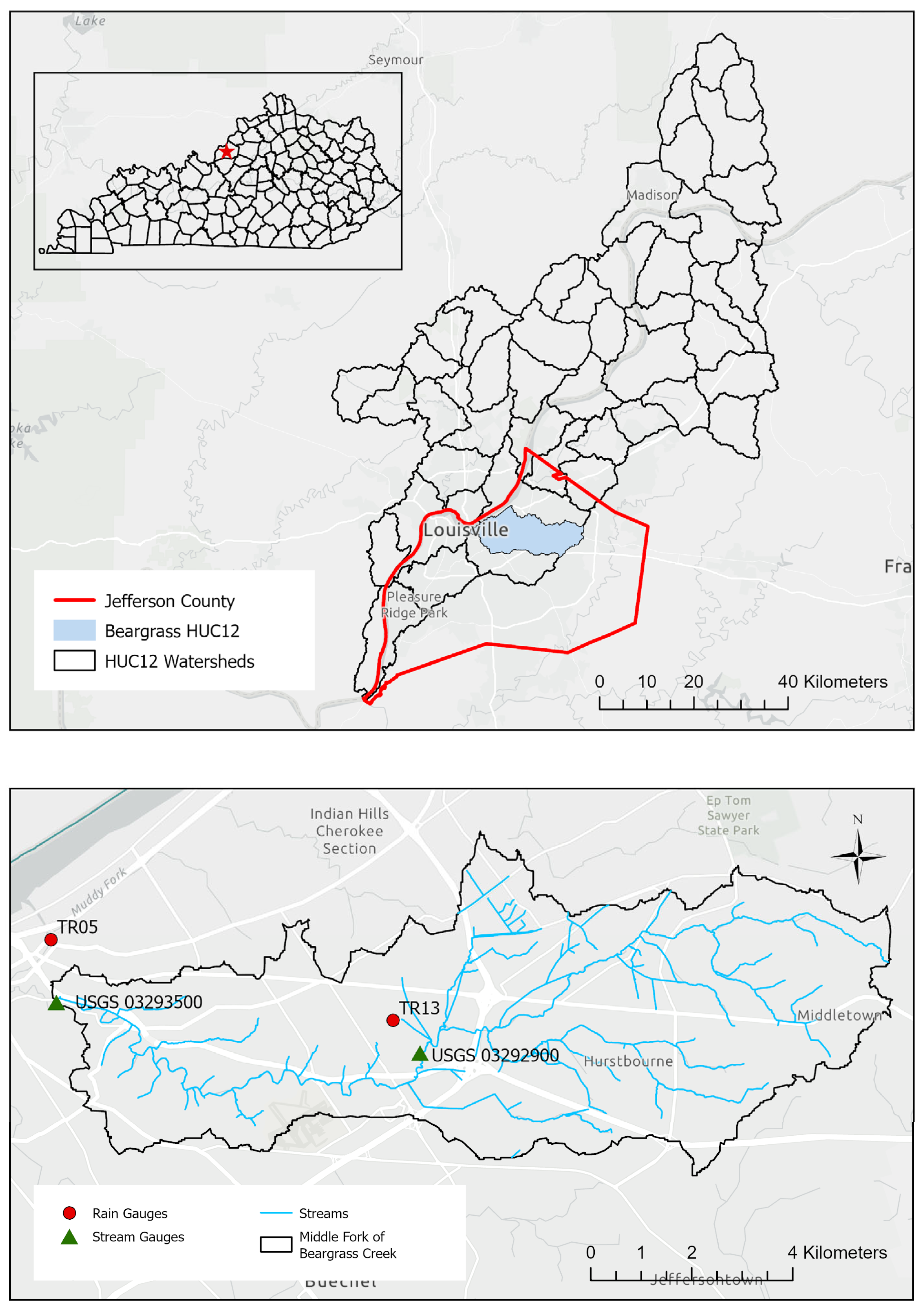
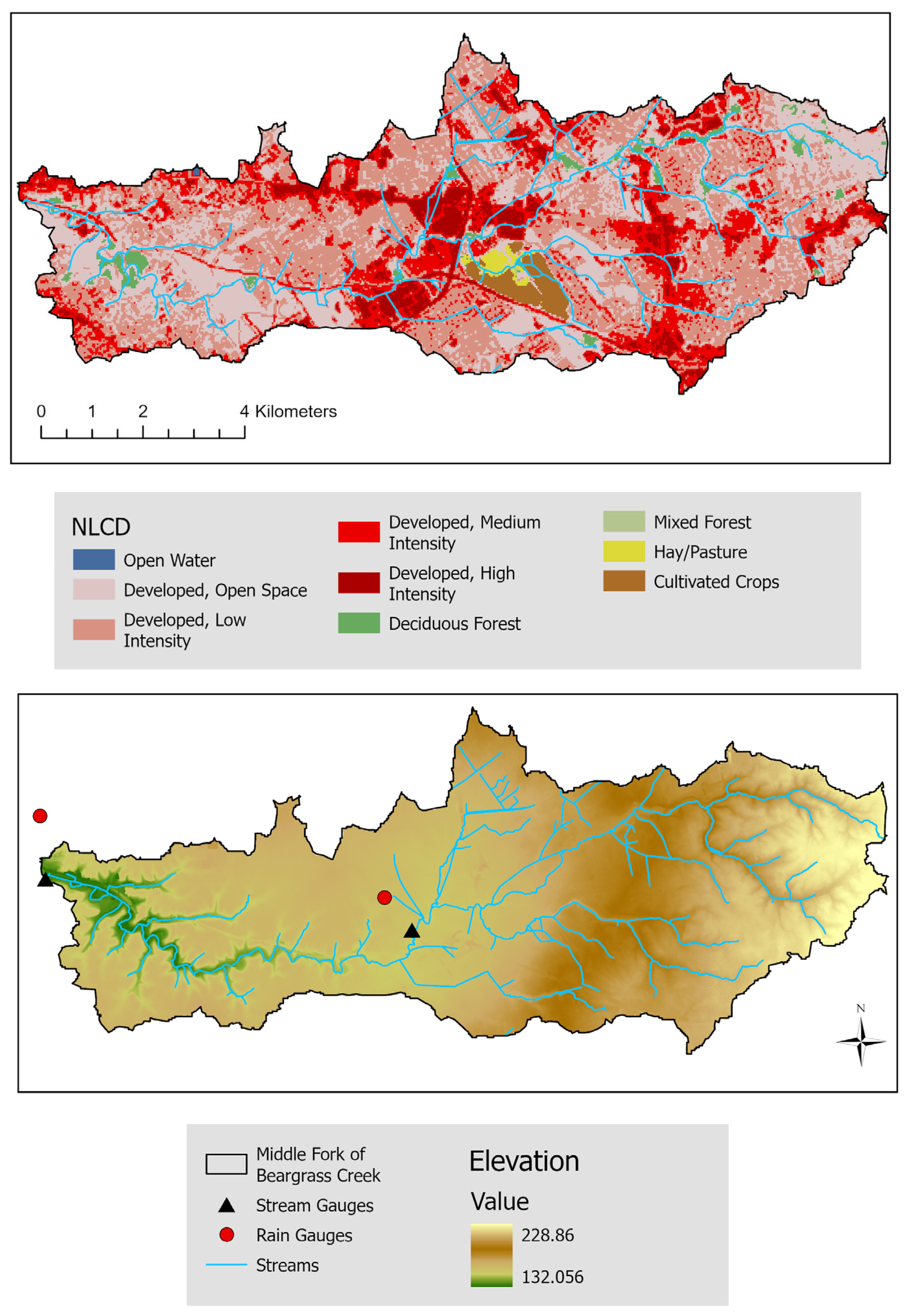
The Middle Fork of Beargrass Creek drains approximately 65 km² in north-central Jefferson County, within the city of Louisville, Kentucky, as part of the larger Silver-Little Kentucky watershed (Figure 1). The headwaters originate near Middletown and flow west through St. Matthews and the park corridor (Seneca and Cherokee Parks) before joining the South Fork near downtown Louisville. Communities within the watershed include the Highlands, Seneca Gardens, St. Regis Park, St. Matthews, Lyndon, Wildwood, Hurstbourne, Douglass Hills, and Middletown [41].

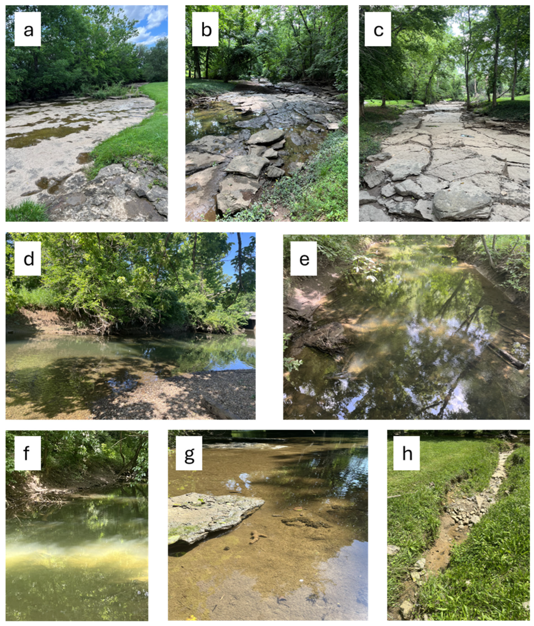
Topographically, the basin lies in Louisville’s Eastern Uplands, characterized by broad, steep-sided valleys and gently rolling plateaus, with elevations ranging from ~229 m in the upper basin to ~130 m near the confluence (Figure 2). Channels are well-entrenched, and near-vertical valley walls are common [41]. The underlying geology consists primarily of lower Devonian and middle Silurian limestones, with some middle Devonian shales, while soils are dominated by Group B drainage classifications with moderate infiltration potential [41]. Land use is primarily residential and commercial, with approximately 37% of the watershed area experiencing impervious surface cover such as roads, rooftops, and parking lots driving rapid runoff generation (Figure 2). Agricultural land is minimal, though remnant parcels such as Oxmoor Farm remain [47]. Limited riparian buffers exist, with green infrastructure largely confined to parks and golf courses [41,48] (Figure 1 and Figure 2).

The climate of Louisville is humid subtropical, with hot, humid summers and cool winters. Thirty-year normals (1991–2020) show an average annual precipitation of 1228 mm and a mean air temperature of 26.6 °C for July and 2 °C for January [49]. Convective storms in summer and frontal systems in cooler months both contribute substantially to annual rainfall with corresponding hydrologic responses typical of urban streams [50].

Inevitably for an urban watershed, some runoff from impervious surfaces in the watershed is routed through a stormwater drainage network that discharges directly into the stream system. Although impervious surfaces reduce the potential for direct rainfall-driven soil detachment from hillslopes, they increase runoff volumes and flow velocities during storm events. These hydrologic changes can enhance channel erosion and mobilization of previously deposited sediments within the stream network. Consequently, turbidity responses observed during storms likely reflect a combination of stormwater runoff, channel erosion, and flushing of stored sediments rather than hillslope erosion alone.

2.3. Storm Identification and Analysis

The Metropolitan Sewer District [51] provided rainfall data from two gauges within the Middle Fork watershed, representing upstream (Up) and downstream (Down) locations, at a 5 min resolution for a two-year period covering June 2023–May 2025 (

Table 1. Stream (USGS) and rain (MSD) gauge information.

USGS Gauge	Area (sq.km)	MSD Gauge	Elev Range (m)	Dominant Landcovers
03293500	64.2	TR05	96.8	Dev Low (41%), Dev Open (28.9%)
03292900	36.8	TR13	75.3	Dev Low (40.3%), Dev Open (25.5%)

and Figure 1). Storm events were identified using three criteria applied sequentially: (1) a 6 h inter-event time definition (IETD), whereby a new storm was initiated whenever at least 360 consecutive minutes without rainfall preceded subsequent precipitation; (2) a minimum storm rainfall amount of 12.7 mm, consistent with values commonly used to identify storms capable of generating measurable runoff and sediment transport. While rainfall intensity is often a key control on erosion processes, this threshold was used only to identify candidate storm events, with rainfall erosivity subsequently quantified using the EI index, which incorporates rainfall intensity [52]; and (3) erosive storms occurring within 48 h of a preceding erosive event were excluded where necessary to minimize the influence of incomplete hydrologic and sediment recovery (e.g., elevated soil moisture, baseflow, and residual turbidity) consistent with event-based hydrologic frameworks that emphasize separation of independent runoff responses [53]. Turbidity responses (see Section 2.4) were also examined to confirm that retained storms represented distinct hydrologic responses. The IETD approach is widely used in hydrologic and water-quality studies to delineate discrete rainfall events [54,55]. Each remaining event was then assigned a unique storm identifier, and only rainfall intervals within storms that occurred at both gauges were retained for subsequent analyses.

For each storm, the following hydrometeorological metrics were calculated following standard rainfall characterization procedures. Total storm accumulation (mm) was computed as the cumulative precipitation during the event. Storm duration (minutes) was calculated as the elapsed time from the first to the last non-zero precipitation record. Maximum 5 min intensity (mm per 5 min) was determined as the highest intensity recorded during the event, and mean event intensity was calculated as total accumulation divided by duration. An intensity peakedness index (Ip) was calculated as the ratio of the maximum 5 min intensity to the mean intensity. The time to peak (Tp) was computed as the fraction of total storm duration elapsed until the maximum 5 min intensity occurred.

For the erosivity index (EI), we first calculated the kinetic energy (e) of each storm (MJ ha⁻¹), using the 5 min rainfall intensity (im) data in mm h⁻¹, taking the form of the equation:

e = 0.29 × [1 − 0.72 × exp(−0.05 × im)]

(1)

which is then multiplied by the rainfall amount (mm) occurring over the same 5 min period and then summed over the length of the storm event for the total storm erosivity index (EI in MJ mm ha⁻¹ h⁻¹) [29,43,52]. The rainfall erosivity index (EI) represents the kinetic energy and intensity of rainfall and therefore characterizes the erosive potential of precipitation itself rather than the erodibility of the land surface. Consequently, EI does not vary with land use conditions such as impervious surfaces; instead, land use influences how rainfall energy is translated into sediment mobilization through its effects on runoff generation, sediment availability, and hydrologic connectivity within the watershed.

To evaluate differences in storm event characteristics between the upstream and downstream gauges, we applied a set of nonparametric statistical tests reflecting the non-normal distribution of the storm datasets. For paired comparisons, in which the same storm event was observed at both gauges, we used the Wilcoxon Signed-Rank Test to determine whether the median of the paired differences (Down−Up) was significantly different from zero. In addition, we conducted unpaired Wilcoxon Rank-Sum Tests to compare the overall distributions of storm metrics between gauges within each meteorological season across the two-year study period. To assess broader seasonal patterns in storm metrics, we applied the Kruskal–Wallis test, a rank-based nonparametric alternative to one-way ANOVA that evaluates differences across more than two independent groups [56]. When the Kruskal–Wallis test indicated significant overall differences (α = 0.05), we conducted Dunn’s multiple comparison and Fligner-Killeen tests to identify specific seasonal contrasts in storm metric medians and variances, respectively [56].

2.4. Turbidity Data and Regression Analysis

The purpose of this modeling framework is to evaluate how upstream turbidity signals and storm characteristics influence downstream turbidity responses during individual storm events, and to quantify the timing and strength of sediment transport connectivity between monitoring locations. The US Geological Survey [57] provided 15 min turbidity data for two stream gauges at upstream (Up) and downstream (Down) locations along the main Middle Fork reach, corresponding to the rain gauge locations and time period (Table 1). Using this data, we modeled downstream turbidity during storm events using an event-based ordinary least squares (OLS) regression framework. Each storm was treated as a unique event, and a separate regression model was fitted to account for variability in storm magnitude, sediment supply, and hydrologic response. For each event, turbidity was modeled as a function of two main predictors: lagged upstream turbidity (turb_up_lag) and lagged downstream rainfall erosivity (EI_down_lag). Upstream turbidity reflects antecedent sediment availability and upstream watershed dynamics, while EI represents the energy of rainfall capable of mobilizing and transporting sediment. This predictor combination follows hydrological studies that highlight the importance of both antecedent conditions and storm forcing in explaining sediment and turbidity responses [16,58].

To align upstream turbidity peaks with downstream responses, we explored a range of plausible travel times between the monitoring stations based on typical transport velocities observed in small stream channels during storm events. This approach reflects the common hydrologic practice of defining a physically reasonable travel-time window for signal propagation between monitoring locations when detailed hydraulic routing information is unavailable. Rather than assuming a single hydraulic velocity, we defined a search window corresponding to velocities between approximately 0.3 and 1.0 m s⁻¹, which encompasses commonly reported flow velocities for small natural and engineered channels under stormflow conditions [59,60]. For the 9.25 km study reach between stream gauges, this range corresponds to potential travel times of approximately 2.5 to 8 h based on the relationship

Travel Time (s) = L/v

where L = 9250 m and v represents the candidate transport velocity. Because streamflow during storm events is inherently unsteady and spatially variable, the selected velocity interval should be interpreted as a physically reasonable envelope used to identify candidate lag structures rather than as a constant hydraulic velocity. For each event, we evaluated lagged upstream turbidity (turb_up_lag) across this window and identified the lag that maximized the adjusted R² of the regression model. Accordingly, the optimal lag was determined empirically from the turbidity time series for each event, with the velocity range serving only to define a physically plausible lag search window. The velocity range used here also reflects typical stormflow conditions for the moderately sloped urban channel reach examined in this study. In steeper headwater catchments, where channel gradients and flow velocities may be higher, shorter travel times would be expected and the appropriate lag-search window would likely shift toward smaller lag intervals. However, the general approach of empirically identifying lags between upstream and downstream signals remains applicable across stream types provided that the lag window is adjusted to reflect local hydraulic conditions.

To represent rainfall erosivity (EI), we used the same approach as in Equation (1) but converted the rainfall data into 15 min periods to correspond with the turbidity data. To account for delays between rainfall input and sediment delivery at the downstream gauge, we tested EI lags ranging from 0 to 4 h (i.e., 0–16 period intervals). This range reflects the expected time between rainfall onset, runoff generation, sediment detachment, and arrival of sediment-laden flow at the gauge [61]. For each storm, we selected the EI lag that, when combined with the best upstream turbidity lag, yielded the highest adjusted R².

To complement the model, we also calculated a lagged turbidity ratio at each time step:

Turbidity Ratio_t = T_down,t/T_up,t−τ

(2)

where T_down,t is downstream turbidity at time t, and T_up,t−τ is upstream turbidity at the best-fit lag τ. This ratio helps identify amplification, attenuation, or new sediment contributions between monitoring locations. Similar approaches have been used in sediment transport research to assess signal propagation and sediment fate in-channel [58,62].

Because turbidity time series often violate classical OLS assumptions due to possible autocorrelation and heteroskedasticity, we applied Newey-West heteroskedasticity and autocorrelation consistent (HAC) standard errors to all regression models. HAC estimation provides robust standard errors and hypothesis tests when residuals exhibit serial correlation or non-constant variance, while retaining the unbiasedness of OLS coefficient estimates [63,64]. Additionally, to assess multicollinearity among predictors, we calculated variance inflation factors (VIFs) for all regression models. VIF values greater than 4 were considered indicative of moderate multicollinearity, and values above 10 as severe multicollinearity [56]. For each storm event, model outputs included the optimal lags, model coefficients, standardized betas, adjusted R², HAC-corrected p-values, and Down gauge turbidity predictions.

2.5. Model Sensitivity and Robustness Analysis

To assess how sensitive the event-based regression models were to the assumed timing between upstream and downstream turbidity signals, we conducted a structured lag-sensitivity analysis for each storm event. Lagged and event-scale variability in turbidity and suspended sediment are well documented in hydrologic systems, arising from travel-time delays, sediment availability, and hysteretic source-response dynamics during storms [65,66]. For each event, initial optimal lags for upstream turbidity and downstream erosivity (EI) were identified, after which a lag window of ±2 time steps were defined around each optimum. This produced a grid of 25 lag combinations for each event, and a standardized linear regression model was fitted for each combination using downstream turbidity as the response and the lagged predictors as covariates.

For each event, the range of adjusted R² values along with standardized regression coefficients (β) for upstream turbidity and downstream EI were extracted across all lag combinations. The mean and standard deviation (SD) of each β distribution were then calculated to quantify the robustness of each predictor’s influence to lag selection. Predictors were classified as very stable (SD < 0.10), moderately stable (0.10 ≤ SD < 0.20), lag-sensitive (0.20 ≤ SD < 0.30), or highly unstable (SD ≥ 0.30) based on predefined thresholds of coefficient variability. This procedure reflects established hydrologic understanding that turbidity and sediment responses can shift markedly depending on event timing, runoff sequencing, and sub-daily sediment transport processes [65,67]. Evaluating predictor behavior across a realistic lag window, therefore, allowed us to distinguish events where upstream turbidity and downstream erosivity exerted a consistent influence from those where the inferred relationships were strongly dependent on lag specification.

2.6. Hysteresis Analysis

We applied a hysteresis analysis to provide additional insights into sediment and particulate transport dynamics during storm events. Hysteresis loops were constructed by plotting the 15 min turbidity data against the corresponding discharge for each event at the downstream gauge only (as discharge is not recorded by the upstream gauge), enabling characterization of temporal lags between flow response and particle mobilization [68]. Whereas the regression framework quantified the relative contributions of upstream turbidity and downstream storm erosivity to downstream turbidity response, and the turbidity ratio captured event-scale differences in source dominance, the hysteresis approach allowed us to further evaluate within-event dynamics and source timing. Strong hysteresis with clockwise loops, where turbidity peaks on the rising limb, typically indicates rapid mobilization of near-channel or urban surface sources, while counterclockwise loops suggest delayed delivery from upstream or distal sources [69]. Quantitative indices such as the hysteresis index (HI) and loop area [45,70,71] were subsequently used alongside regression outputs to provide a more holistic understanding of storm-driven turbidity behavior. Together, these methods allowed event-scale characterization of both between-event variability (via regression and turbidity ratios) and within-event transport dynamics (via hysteresis), thereby strengthening inference on sediment source pathways and controls in the study watershed.

3. Results

3.1. Storm Characteristics and Seasonality

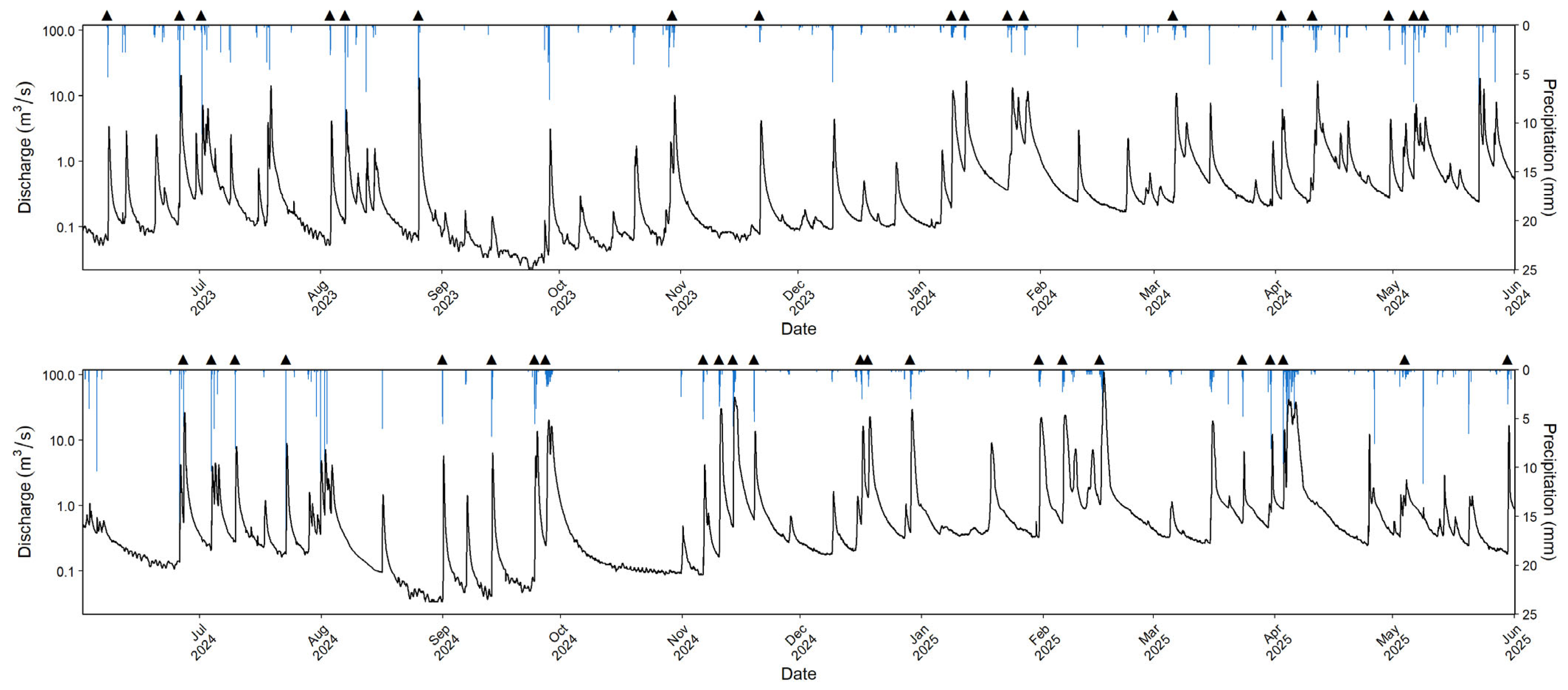
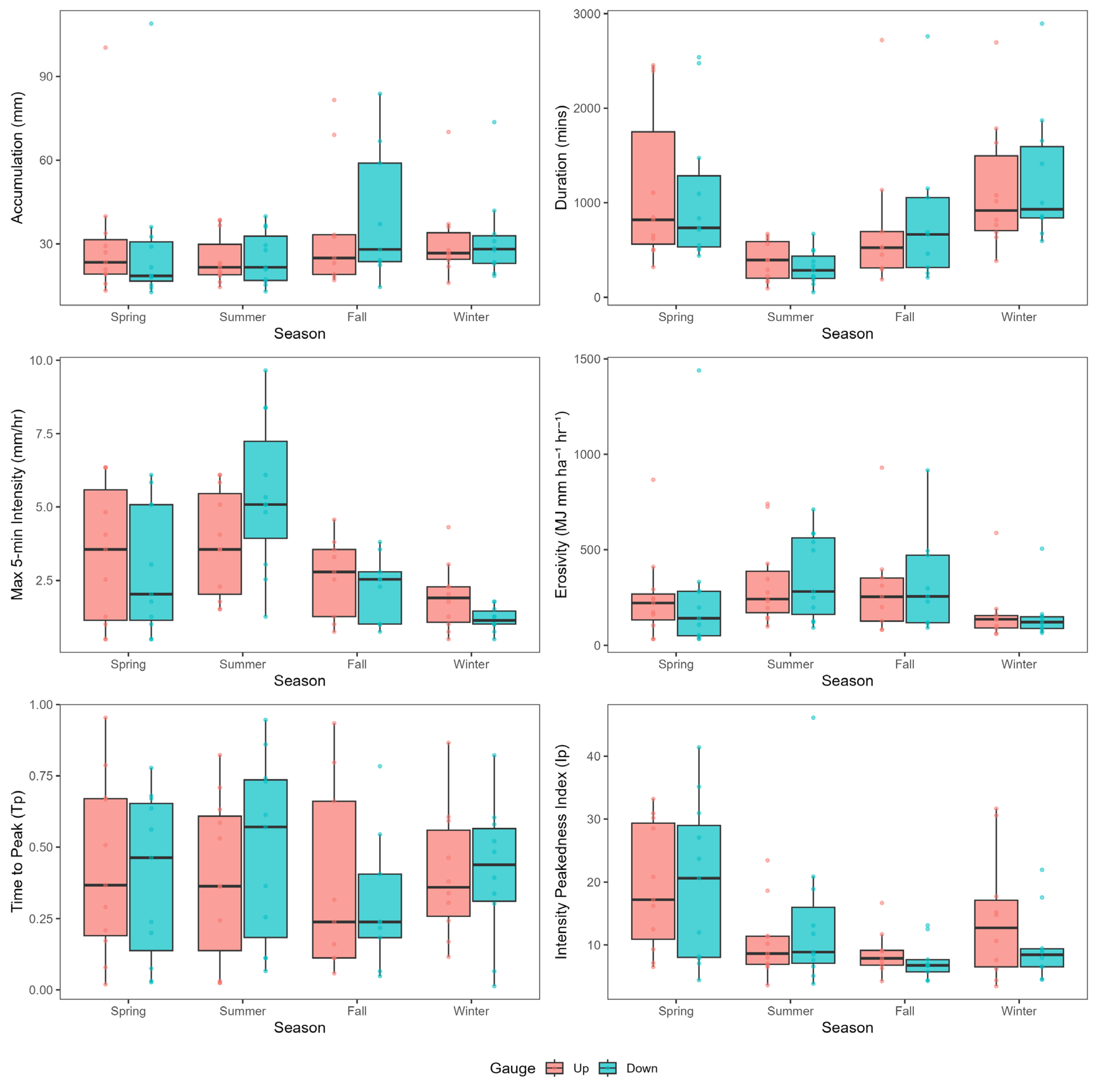
Screening of the rainfall data resulted in 41 separate erosive storm events extracted at each gauge between June 2023 and May 2025. Figure 3 highlights each event in line with the 15 min Down gauge precipitation and discharge. Figure 4 displays boxplots of the key storm characteristics for both gauges by season. Storm characteristics displayed clear and consistent seasonal patterns at both the upstream (Up) and downstream (Down) gauges, with strong agreement in the structure and magnitude of seasonal contrasts. Nonparametric tests (Kruskal–Wallis and Fligner-Killeen) were used to identify which seasonal differences in medians and variances were statistically significant. While some differences in characteristics between gauges were apparent, these were not statistically significant based on the Wilcoxon test outputs.

3.1.1. Storm Duration

Storm duration showed some of the most pronounced seasonal changes. At both gauges, durations were longest during winter and spring and shortest during summer. Mean durations at the Up gauge exceeded 1100 min in winter and spring, compared to approximately 385 min in summer, and the Down gauge showed the same cold-season-warm-season divide. Variability in duration was also greatest during winter and spring at both stations. The Kruskal–Wallis test indicated significant seasonal differences in median duration at both the Up and Down gauges (p < 0.01). Post hoc tests showed that spring storms had significantly higher median durations than summer storms at both gauges. No significant seasonal differences in duration variance were detected at either gauge.

3.1.2. Storm Erosivity

Storm erosivity (EI) exhibited a strong warm-season peak, with summer storms producing the highest mean and median erosivity values at both gauges. Spring and fall events showed intermediate levels, and winter storms consistently had the lowest erosivity. Although these patterns were clear descriptively, the Kruskal–Wallis and Fligner-Killeen tests did not detect statistically significant seasonal differences in median or variance for erosivity at either gauge.

Figure 4. Boxplots of storm characteristics by rain gauge and season.

Figure 4. Boxplots of storm characteristics by rain gauge and season.

3.1.3. Rainfall Intensity

Short-interval rainfall intensities, captured by the 5 min intensity and ratio of max 5 min intensity to mean 5 min intensity (Ip), also showed pronounced seasonal differentiation. Both metric means and medians were highest in summer and lowest in fall and winter, with moderate values in spring. Variability in intensity was greatest in spring and summer for both gauges. At the Down gauge, the max 5 min intensity showed significant seasonal variation in both median (p < 0.001) and variance (p < 0.001). Pairwise comparisons indicated that summer storms had significantly higher median 5 min intensities than winter storms, while variance was significantly higher in spring than in winter. At the Up gauge, max 5 min intensity showed significant differences in variance across seasons (p < 0.01), although no individual pairwise contrasts were identified. The ratio of max 5 min intensity to mean 5 min intensity (Ip), despite showing clear seasonal structure descriptively, did not show statistically significant median or variance differences in the statistical tests for either gauge.

3.1.4. Storm Accumulation

Storm accumulation demonstrated minimal seasonal differences. Mean and median accumulations were generally larger in winter and spring, intermediate in fall, and lowest in summer at both gauges. Although the Up gauge tended to record slightly higher mean accumulations across seasons, these differences were small, and neither the Kruskal–Wallis nor Fligner-Killeen tests found significant seasonal differences in medians or variances at either gauge.

3.1.5. Time to Peak

The ratio of time to storm peak to storm duration (Tp) displayed similar variability across all gauges and seasons. Fall displayed consistently lower mean and median Tp values, indicating a tendency for right-skewed storms that peak earlier in their durations, while the Up gauge also generally recorded lower Tp values across all seasons. Nonetheless, statistical testing did not detect significant seasonal differences in Tp medians or variances at either the Up or Down gauge.

3.2. Turbidity Regression Model

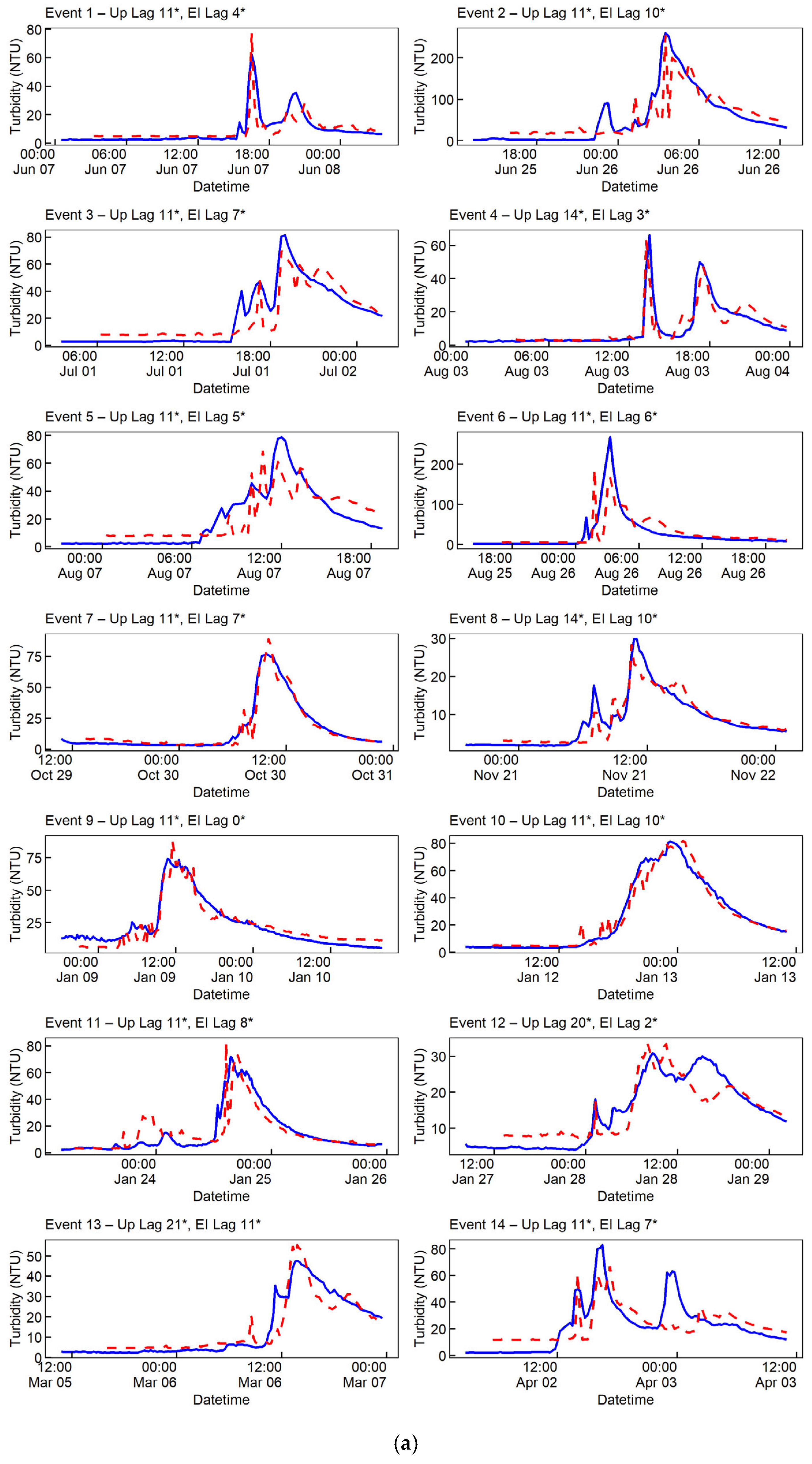
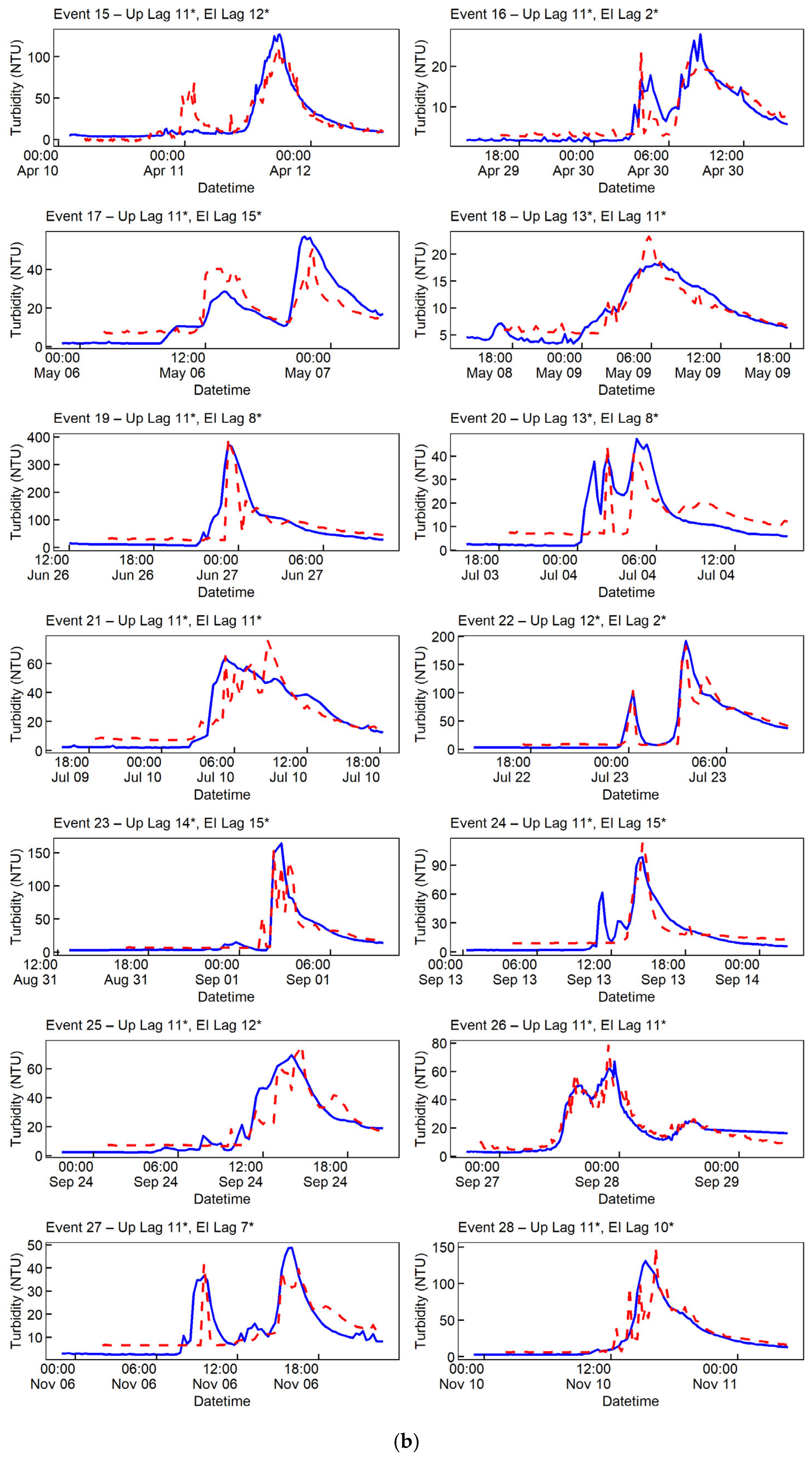
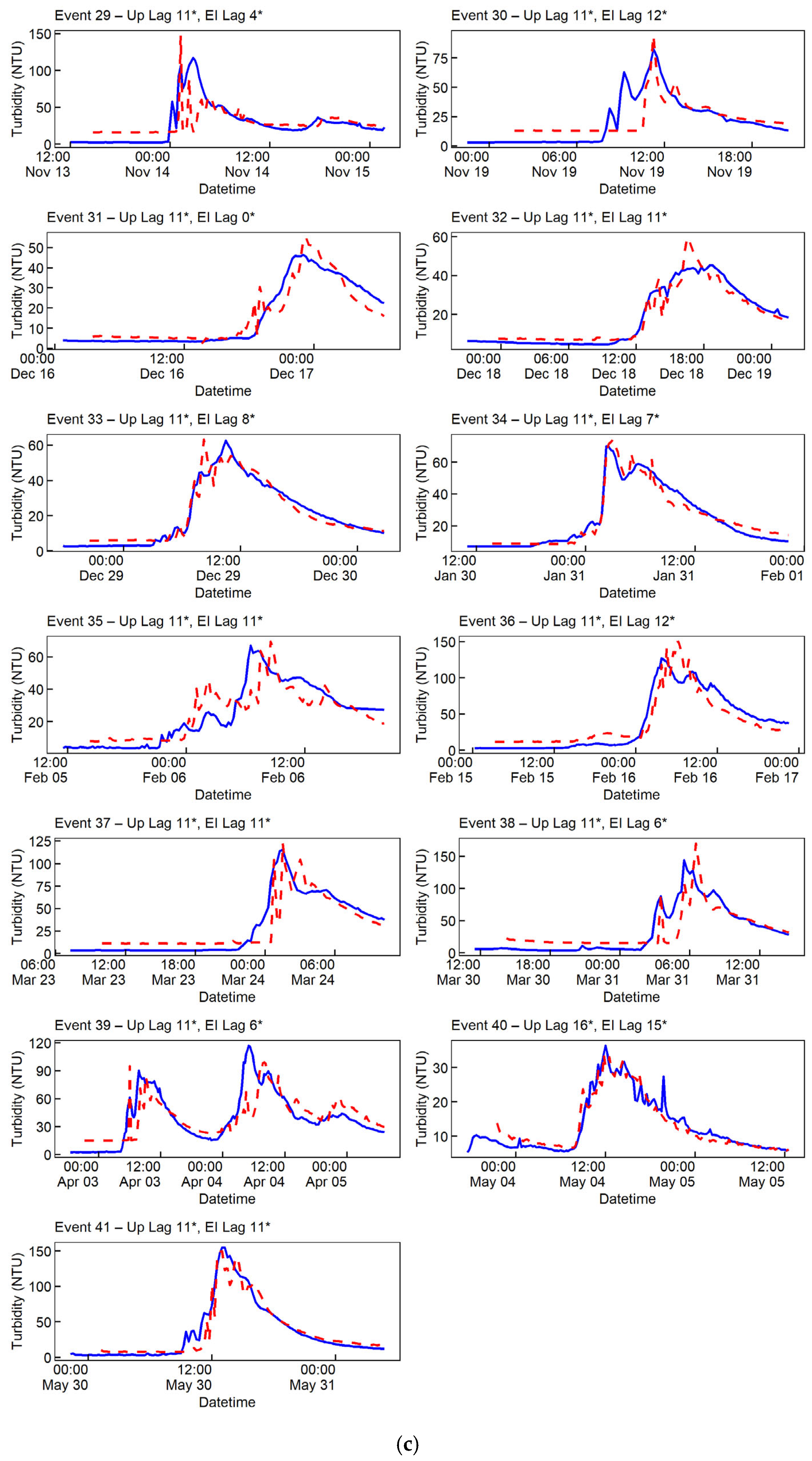
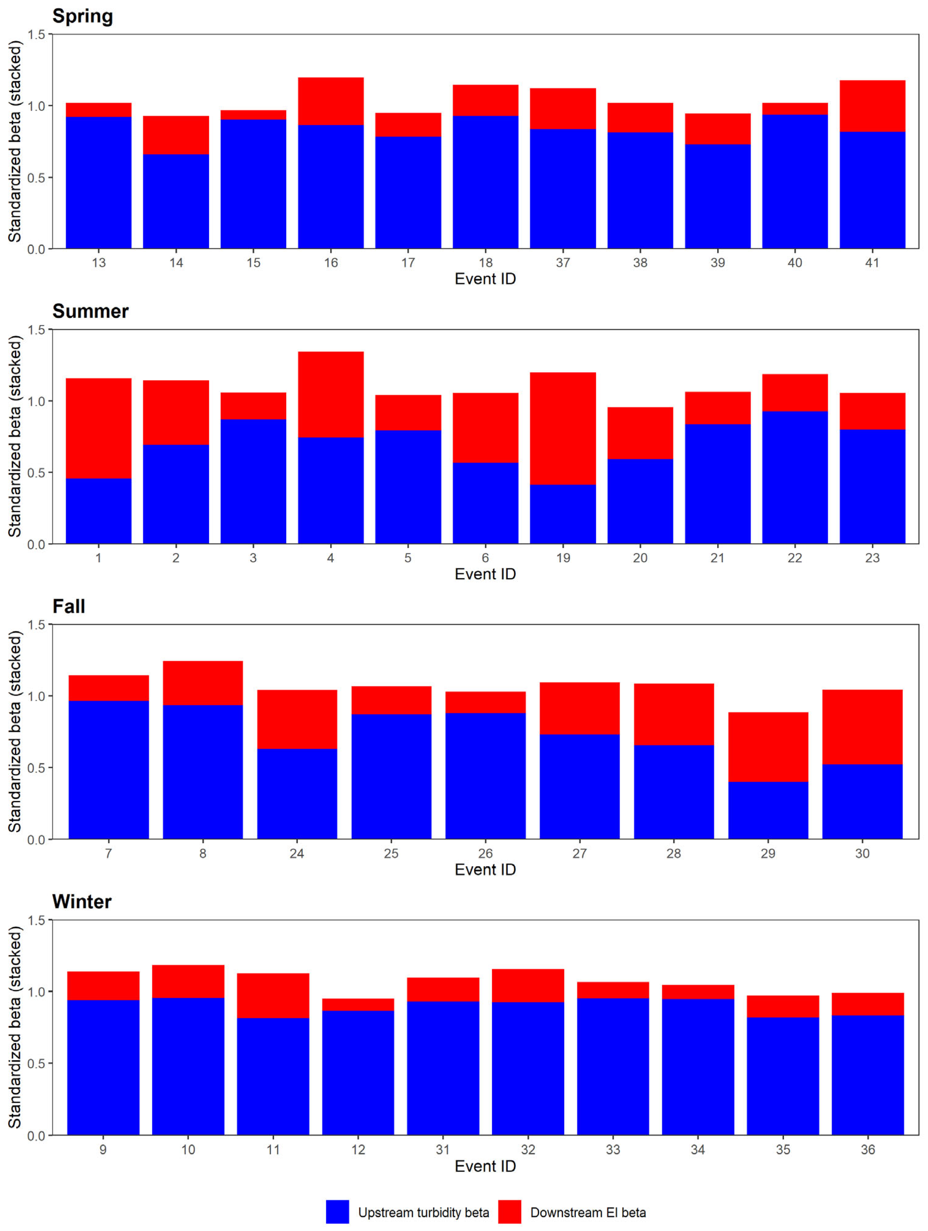
Across the 41 storm events included in the analysis, the OLS regression models consistently identified lagged upstream turbidity (turb_up_lag) and lagged downstream storm erosivity (EI_down_lag) as influential predictors of downstream turbidity (Figure 5a–c). Both predictors were statistically significant (p < 0.05) in all modeled events, indicating that each variable provided independent explanatory strength across a wide range of storm conditions. Overall model performance was generally strong, with adjusted R² ranging from 0.34 to 0.95 and a mean of 0.73.

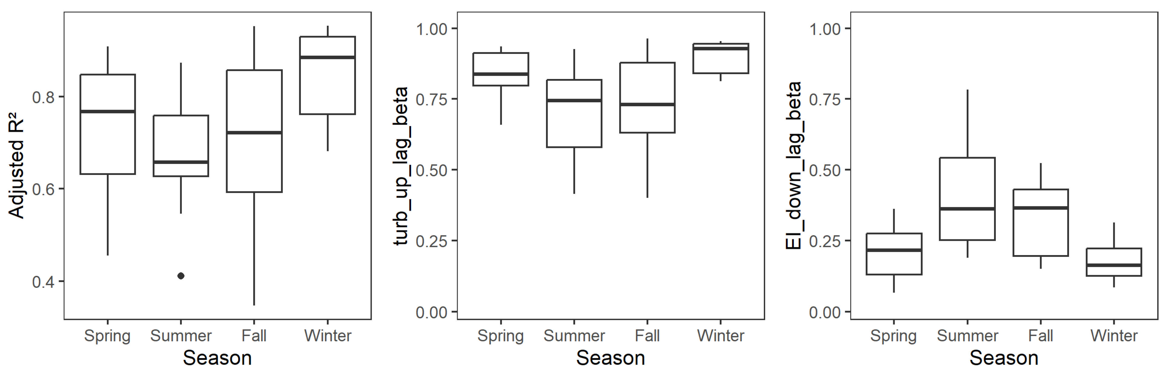
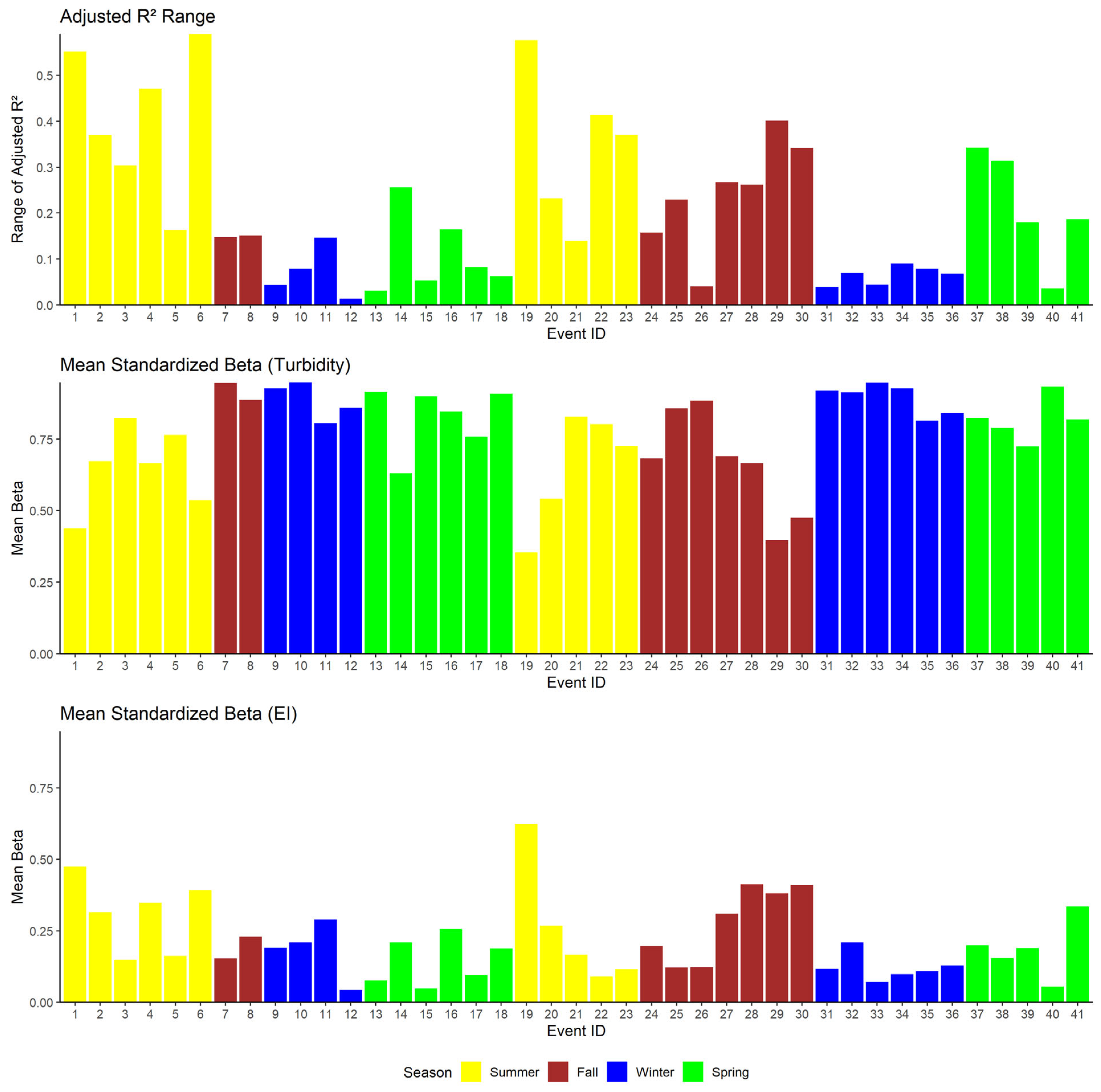
Clear seasonal patterns were evident in the model statistics. Winter events exhibited the highest mean adjusted R² (0.85), followed by spring (0.74) and fall (0.72), while summer events showed the lowest mean R² (0.68) (Figure 6). Standardized effect sizes (beta β coefficients) further highlighted seasonal differences. The influence of lagged upstream turbidity (turb_up_lag) was consistently strong, with positive standardized coefficients in all events. The seasonal mean effect sizes were winter: 0.898, spring: 0.835, fall: 0.732, summer: 0.699 (Figure 6 and Figure 7). Thus, lagged upstream turbidity (turb_up_lag) had the strongest standardized influence in winter and the weakest influence in summer, but remained a major predictor across all seasons.

The effect of lagged downstream erosivity (EI_down_lag) also varied seasonally. The mean standardized coefficients were summer: 0.414, fall: 0.339, spring: 0.179, winter: 0.142 (Figure 6 and Figure 7). The erosivity predictor, therefore, exhibited the strongest relative influence in summer and fall, with smaller effects in spring and winter, though it remained statistically significant in every event regardless of season. Variance inflation factors (VIFs) for both predictors were consistently near 1.0 in all events, indicating extremely low multicollinearity and confirming that the predictors contributed independently to model performance.

3.3. Model Robustness and Sensitivity

To evaluate the temporal stability of the regression models across storm events, we conducted a lag-sensitivity analysis by varying lagged upstream turbidity (turb_up_lag) and lagged downstream erosivity (EI_down_lag) predictors by ±2 lag timesteps. For each event, the range of adjusted R² across lag combinations (ΔAdjusted R²) was used to assess the model’s sensitivity to timing assumptions. Based on guidance from hydrologic modeling literature, we categorized events as stable (ΔR² ≤ 0.2), moderately sensitive (ΔR² = 0.2–0.4), or highly sensitive (ΔR² > 0.4). Previous studies emphasize that relatively small changes in fit metrics often fall within typical model uncertainty, whereas larger variations across model configurations can indicate meaningful differences in process representation or structural equifinality [72,73,74,75].

Most storm events fell within the stable category, exhibiting ΔR² values below 0.2 (Figure 8). This suggests that, for these events, model performance and predictor influence were relatively insensitive to moderate shifts in lag structure, supporting the consistency of the lagged turbidity-erosivity model structure. These events also exhibited consistent positive standardized coefficients for lagged upstream turbidity with generally lesser, but still meaningful contributions from lagged downstream erosivity (Figure 8). Moderately sensitive events (12 in total) exhibited ΔR² values between 0.2 and 0.4, representing a transitional category where lag timing modestly influenced model fit. By contrast, five events (1, 4, 6, 19, 22—all summer events) exhibited ΔR² values exceeding 0.4 (Figure 8). These highly sensitive events showed dramatic changes in model performance and standardized coefficients with small shifts in lag choice, suggesting that the temporal alignment between drivers and downstream turbidity may be poorly defined or unstable, potentially due to additional, unmodeled processes such as local erosion or urban infrastructure that are not captured by upstream turbidity or erosivity metrics alone.

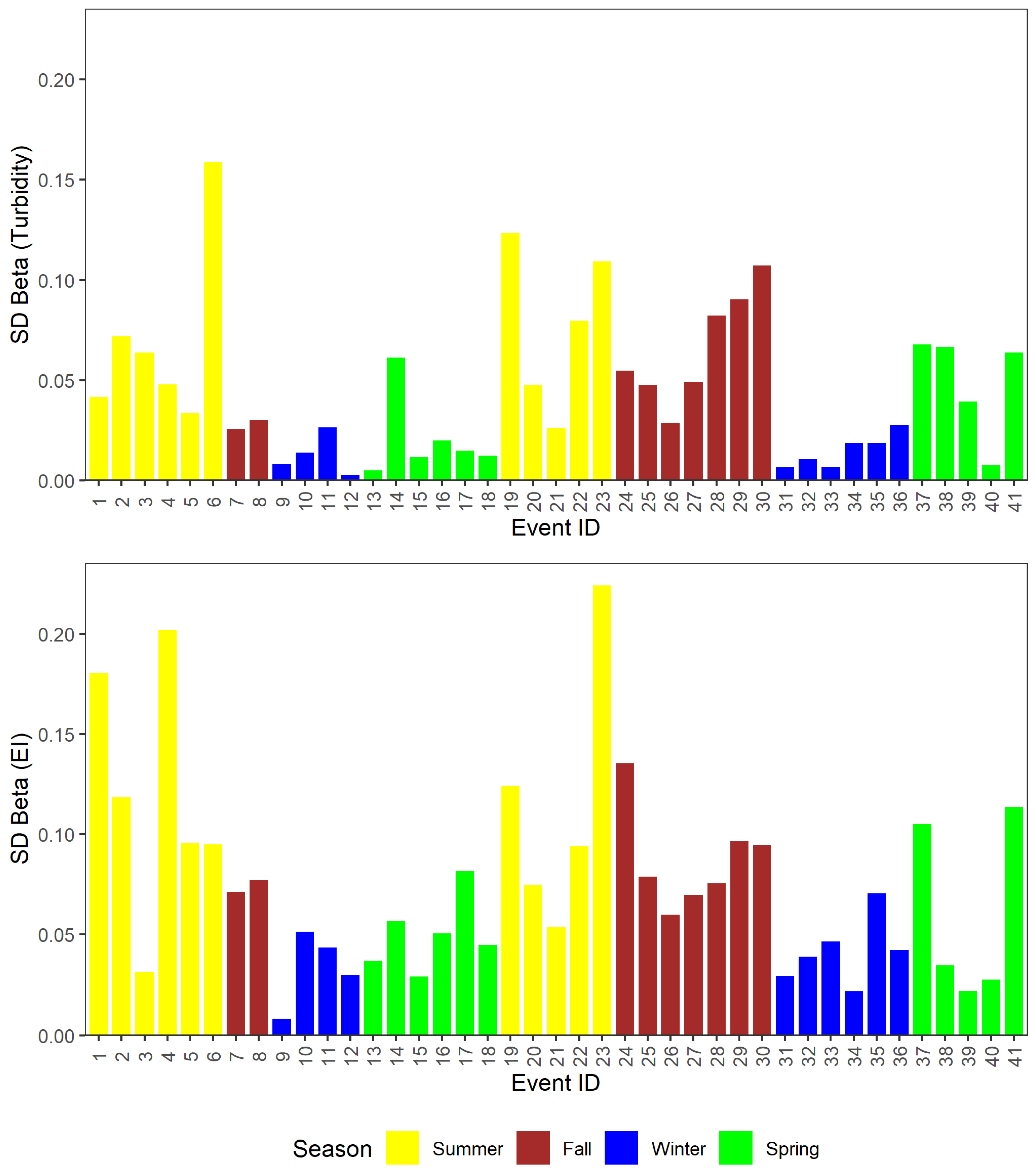
In addition to overall model fit, we examined the stability of standardized regression coefficients (β) for both upstream turbidity and downstream erosivity across the tested lag combinations. Events were classified based on the standard deviation (SD) of β as follows: very stable (SD < 0.10), moderately stable (0.10 ≤ SD < 0.20), lag-sensitive (0.20 ≤ SD < 0.30), and highly unstable (SD ≥ 0.30). These thresholds were chosen to reflect increasing sensitivity of regression coefficients to lag selection, consistent with prior studies showing that large parameter variability across model configurations indicates structural or timing dependence rather than random noise [72,73]. All events displayed stable to moderately stable lag sensitivity for upstream turbidity, while only two events (4 and 23) showed lag-sensitive downstream EI influence (SD = 0.20 and 0.22), despite very to moderately stable upstream turbidity (SD = 0.05 and 0.11) (Figure 9). Both events occurred during the summer season and were characterized by short durations and high rainfall intensities relative to other storms in the dataset.

Most events exhibited parallel trends, where variability in model fit was accompanied by corresponding shifts in β values. However, certain events demonstrated a decoupling of these behaviors, offering further insight into the role of timing in model robustness. An illustrative case is Event 19, which exhibited a large range in adjusted R² across lag combinations (ΔAdjusted R² > 0.4), indicating that model performance was highly sensitive to the timing assumptions applied to upstream turbidity and downstream erosivity inputs. However, despite this variability in fit, the standardized coefficients (β) for both predictors remained moderately stable, with standard deviations below 0.2. This apparent contrast reflects a key distinction: while the overall explanatory power of the model depended on proper lag alignment, likely due to sharp peaks or faster sediment transport during the event, the relative influence of upstream turbidity and downstream erosivity on downstream turbidity remained consistent across time shifts. This summer storm generated the largest turbidity peak observed at both gauges in the dataset.

Such a pattern of decoupling between model sensitivity (ΔR²) and coefficient stability (β) suggests that the underlying processes governing storm-driven sediment transport, as inferred from turbidity behavior during Event 19, were stable in structure but sensitive in timing. That is, the predictors reliably contributed to turbidity regardless of lag, but the degree of explained variance (R²) depended heavily on matching the model’s timing with the arrival of the sediment-associated turbidity signal at the downstream site. This phenomenon is consistent with events characterized by rapid hydrologic response or short travel times, where slight lag mismatches can obscure otherwise strong relationships. Accordingly, Event 19 highlights the importance of distinguishing between model sensitivity in fit (ΔR²) and stability in predictor interpretation (β). Events with high ΔR² but stable β are likely suitable for inference on sediment transport drivers but require careful lag specification to ensure predictive accuracy.

3.4. Turbidity Ratios

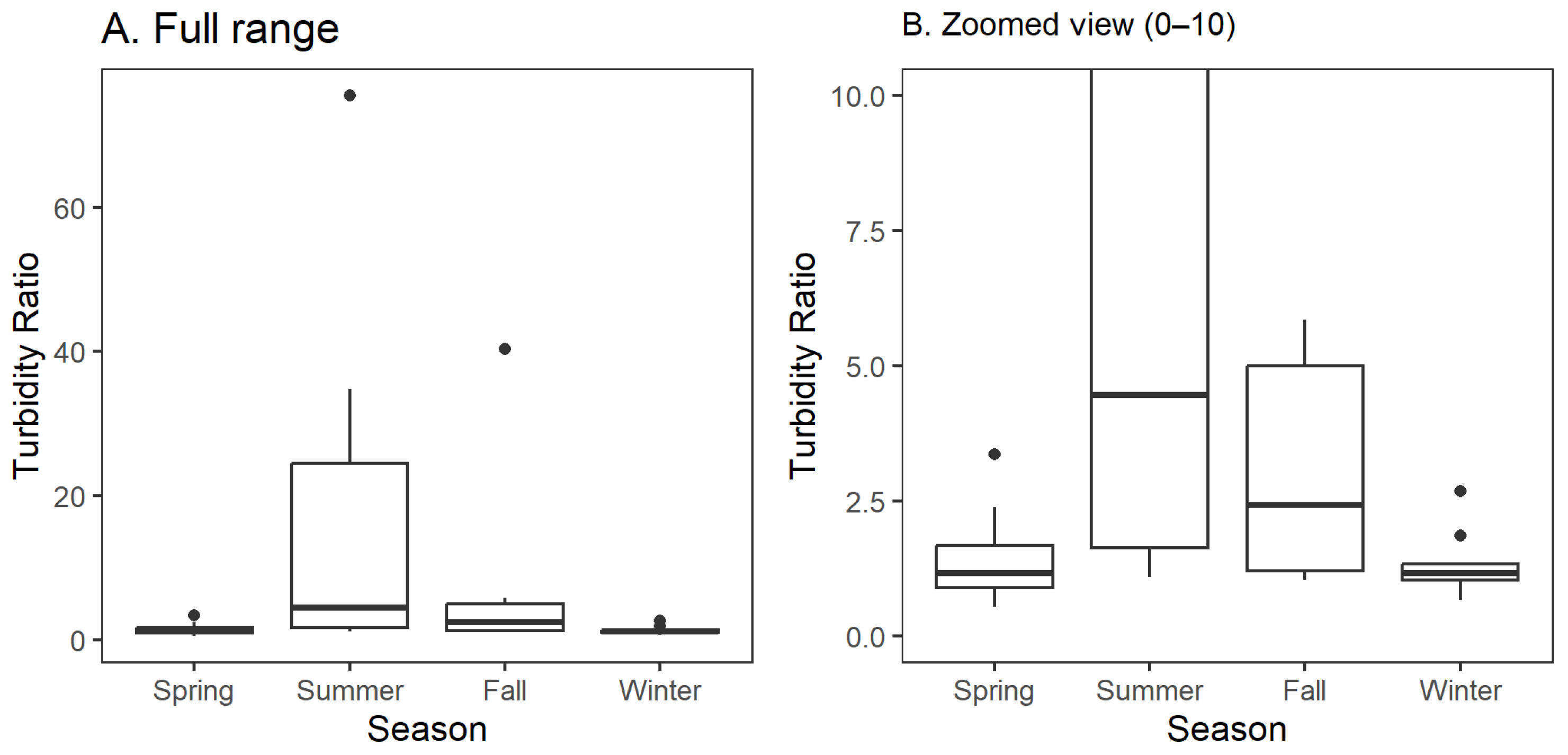
Downstream turbidity peaks were typically higher than the corresponding lagged upstream values, with turbidity ratios spanning more than two orders of magnitude. Ratios ranged from 0.54 to 75.5, with a strongly right-skewed distribution (median 1.42; mean 6.5). Most events exhibited modest amplification from upstream to downstream, but a small number of storms produced extremely high ratios (>30), indicating strong turbidity generation or storage-release processes within the intervening channel reach.

Seasonal patterns were evident in both the magnitude and variability of turbidity ratios (Figure 10). Summer and fall events showed the highest ratios overall, driven by several storms with low upstream turbidity, yet sharp downstream peaks. These extreme cases suggest localized sediment mobilization independent of upstream conditions, potentially linked to dry antecedent periods or high-intensity convective rainfall typical of late summer. In contrast, winter and spring events generally exhibited lower and more constrained ratios, reflecting greater synchrony between upstream and downstream turbidity responses and more continuous sediment availability under wetter seasonal conditions.

Storm erosivity (EI) also co-varied with the turbidity ratio patterns. Both Up and Down EI values were highest in summer and fall, consistent with the clusters of high-ratio events in these seasons. Even where upstream EI was elevated, high ratios occurred primarily when upstream turbidity remained low while downstream turbidity spiked, suggesting that erosive energy was concentrated in the downstream sub-watershed or that local sediment sources were activated independently of upstream contributions. Conversely, winter events characterized by lower EI and more uniform runoff generation produced turbidity ratios closer to one, indicating that downstream turbidity largely mirrored upstream inputs with limited additional sediment mobilization.

3.5. Hysteresis Analysis

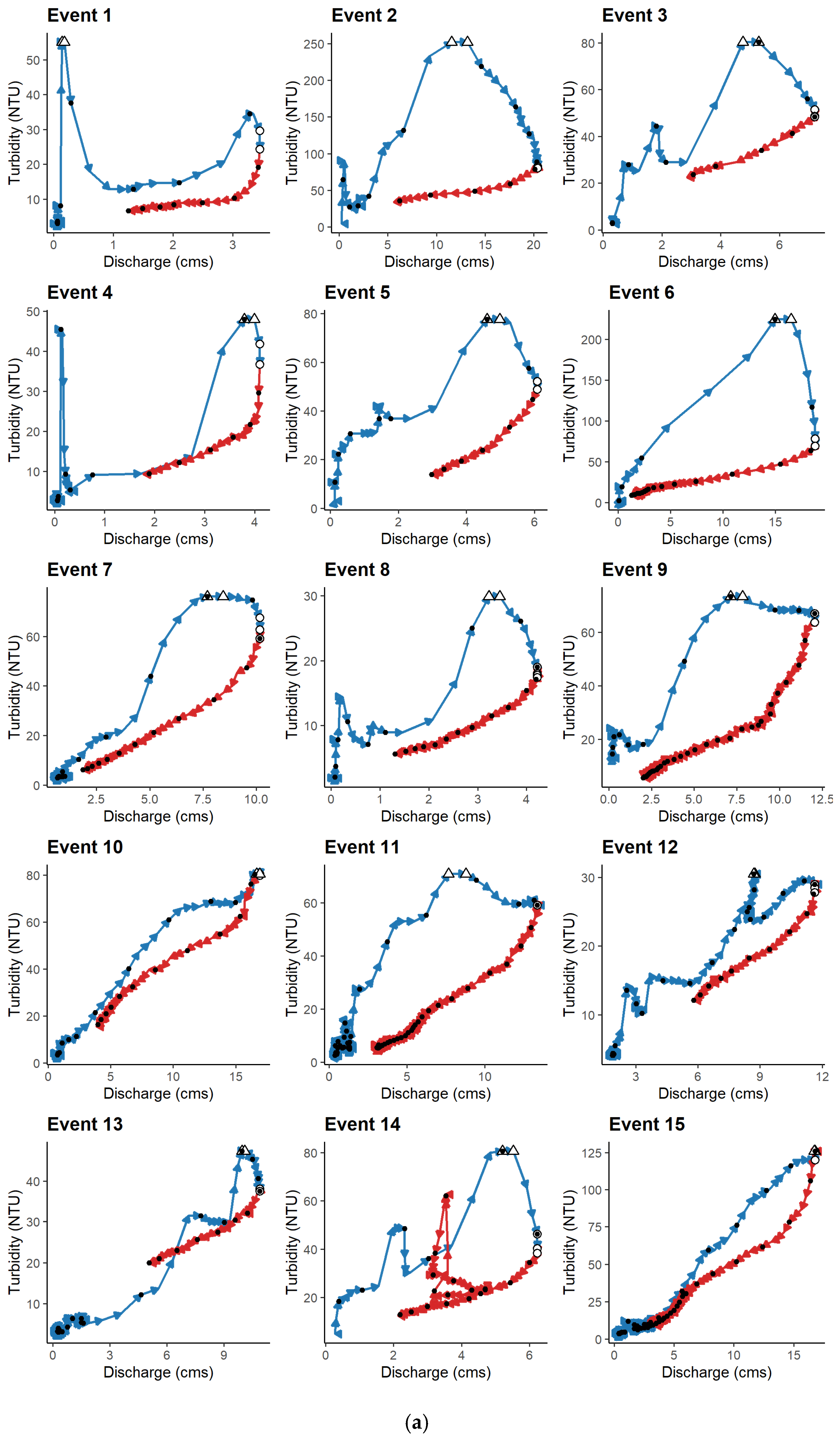
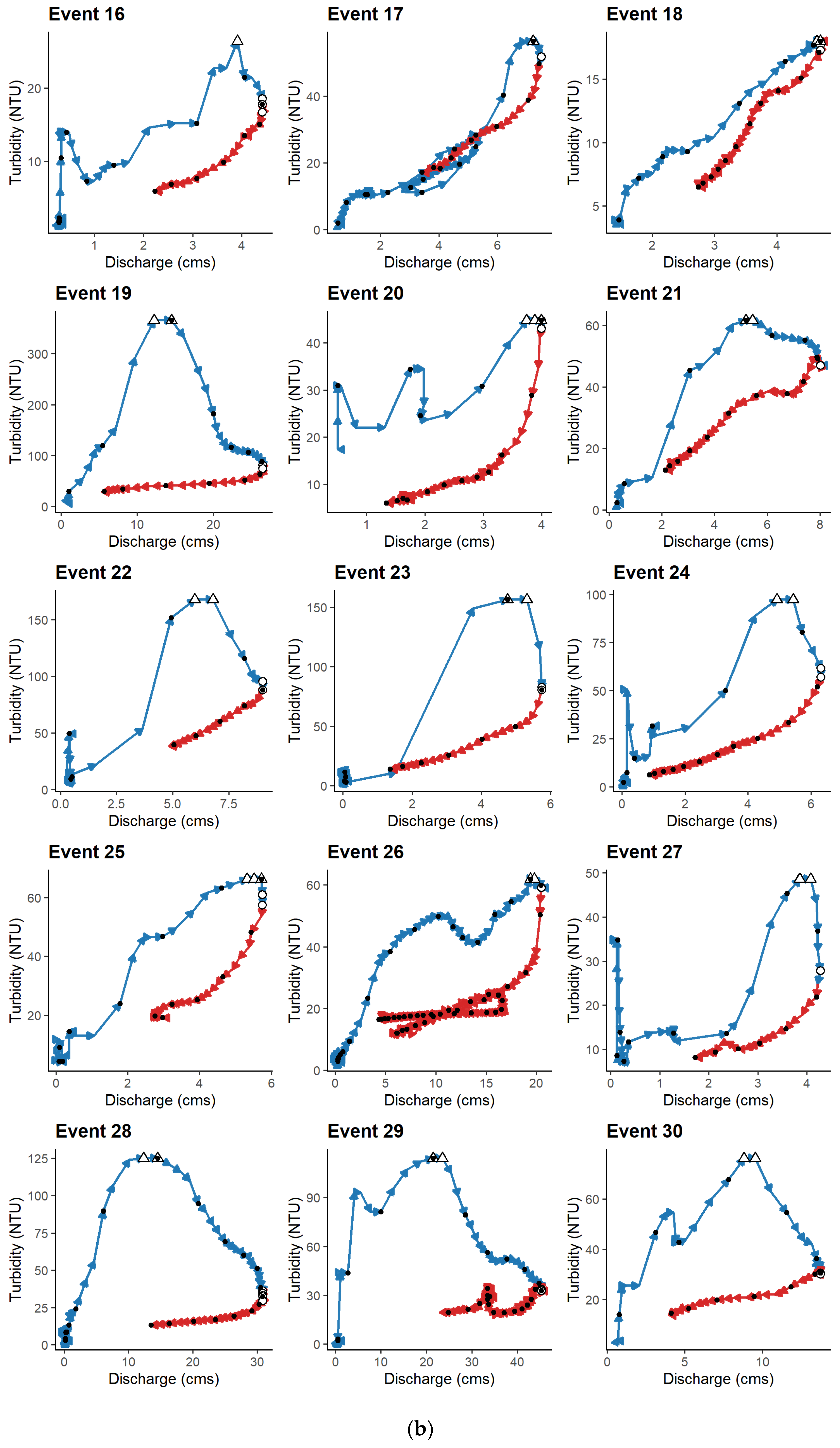
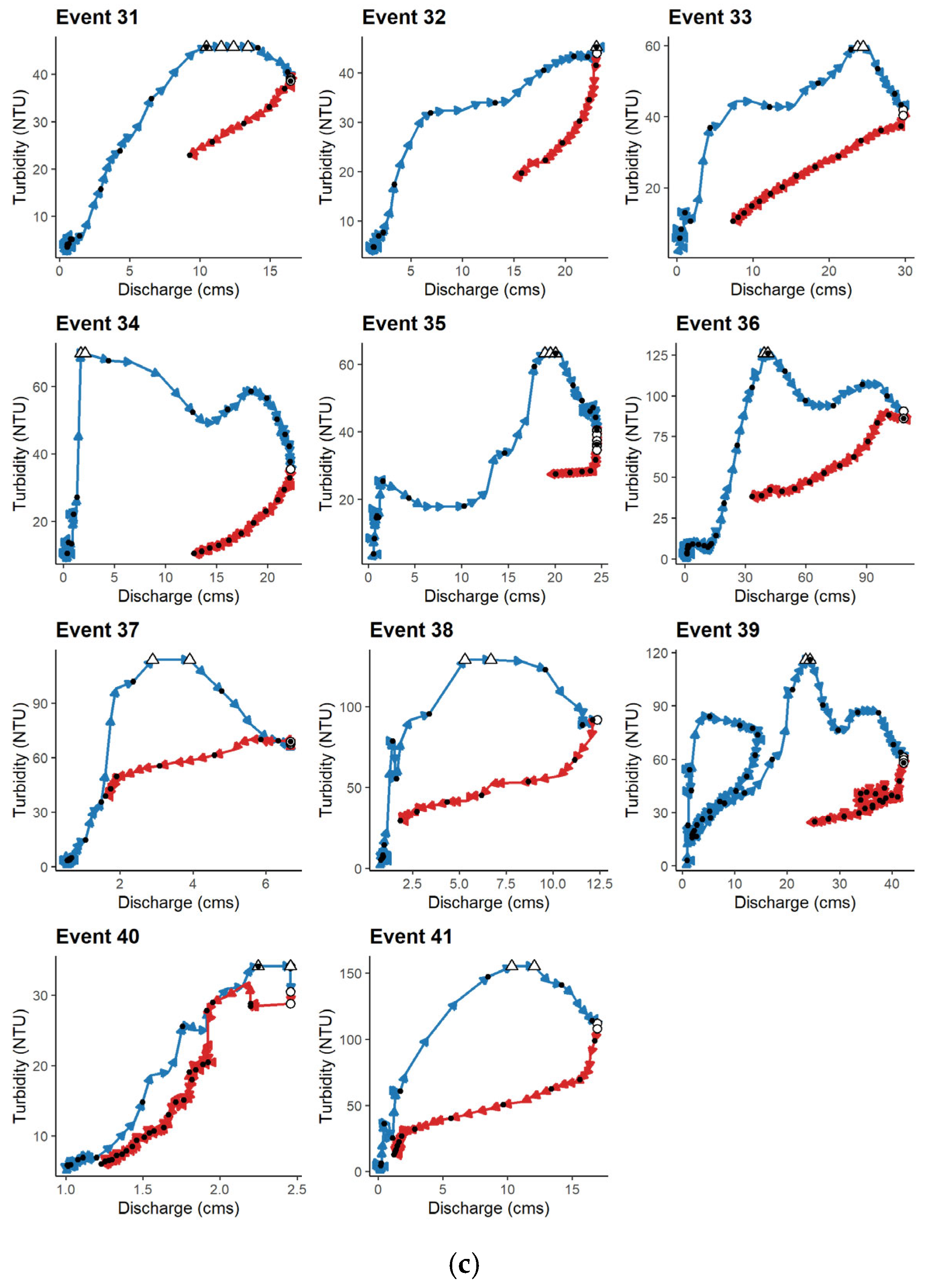
Hysteresis analysis revealed consistent patterns in turbidity–discharge relationships across the 41 storm events evaluated. All events exhibited clockwise hysteresis, indicating that turbidity generally peaked earlier than discharge in the hydrographs at the Down gauge. Although all events exhibited positive hysteresis indices indicating clockwise behavior, several storms produced more complex loop geometries that may visually appear ambiguous in the turbidity–discharge plots. Such patterns can arise when hydrographs contain multiple discharge peaks or when sediment supply fluctuates during the storm, producing secondary turbidity pulses that distort the apparent loop structure. These dynamics can create irregular or partially overlapping loops while still maintaining an overall clockwise hysteresis direction. Similar complexity in sediment hysteresis has been documented in storm-driven sediment transport studies where multiple sediment sources or sequential runoff pulses influence sediment delivery [69,70].

Peak lags ranged widely across events, from −540 min to −15 min, with a median lag of −105 min, reflecting a characteristic timing offset where turbidity rose and peaked before flow (Figure 11a–c). The Hysteresis Index (HI) values were uniformly positive, ranging from 0.17 to 0.46 (median: 0.32), which corroborates the dominance of clockwise loop direction. Normalized loop areas ranged from near zero to 0.61, with a median of 0.31, indicating that while some storms generated pronounced hysteresis, many exhibited only modest deviations between the rising and falling limbs once storm magnitude was accounted for.

Across seasons, the normalized loop area showed several differences. Fall events exhibited the largest normalized areas on average (mean = 0.37), followed by summer (0.34) and winter (0.32), whereas spring events had the lowest mean values (0.24) and the widest overall range (0.0003–0.49). These seasonal contrasts suggest that the strength of hysteresis—relative to event magnitude—was generally greatest during fall and summer storms, many of which were influenced by short-duration or high-intensity rainfall capable of producing sharp, early turbidity pulses. Winter events showed moderate but variable normalized loop magnitudes, while spring storms tended toward weaker hysteresis once storm size was accounted for. Despite these differences, clockwise directionality persisted across all seasons.

Hysteresis loop morphology was generally simple: 83% of events contained zero secondary turbidity peaks, and no event contained more than two. Only a small subset exhibited multi-peak structures (concentrated across winter–spring), with one event showing two secondary peaks (40) and seven events showing a single secondary peak (17, 26, 27, 32, 34, 38, 39), indicating that most storms involved a single, coherent rise and fall in turbidity. Peak lags were consistently negative in every season, but their magnitudes varied. Summer events displayed some of the earliest turbidity peaks (−240 min or more), whereas fall events exhibited more moderate timing offsets.

4. Discussion

4.1. Seasonal Controls on Turbidity Dynamics

Seasonal controls on erosive storm characteristics exerted a strong influence on the hydrologic responses and sediment transport behavior inferred from turbidity observed in this study, with clear implications for understanding turbidity dynamics across the watershed. Winter and spring storms were characterized by longer durations and greater accumulations, while summer storms were shorter but markedly more intense. This fundamental difference in storm morphology governed the strength and predictability of turbidity responses. Longer-duration winter and spring storms produced clearer and more stable relationships between upstream and downstream turbidity, with regression models showing higher performance and stronger influence from lagged upstream turbidity. These patterns are consistent with enhanced hydrologic connectivity during longer storms, which allow sediment mobilized in upstream tributaries to propagate downstream more coherently, resulting in more predictable turbidity responses [45,70,76]. The behavior of erosive storm characteristics in these seasons appears to facilitate the lag relationships captured by the models.

In contrast, summer storms exhibited the highest rainfall intensities and erosivity values in the dataset, but also the shortest durations. Intense, short-lived convective events can generate sharp, localized increases in turbidity that do not necessarily propagate through the watershed in a manner detectable via upstream lags, reflecting broader evidence that high-intensity, short-duration storms often yield highly localized runoff and erosion responses [77,78]. This was reflected in the regression outputs, where model fits were more variable and summer storms showed significantly higher median max 5 min intensities at the downstream gauge compared to winter, with significantly higher variance in intensity relative to some seasons, indicating a high degree of storm-to-storm heterogeneity. Such variability likely contributes to the reduced predictability of turbidity during summer events.

Downstream erosivity (EI_down_lag) played a more limited and inconsistent role in explaining downstream turbidity across seasons. Although summer storms displayed the highest erosivity values descriptively, neither gauge exhibited significant seasonal differences in erosivity medians or variances in the non-parametric tests. Correspondingly, the regression models only intermittently identified lagged erosivity as a more significant predictor, mainly during high-intensity storms. This suggests that erosivity, while physically related to rainfall energy, may not consistently translate into turbidity response at the lag scales evaluated here, particularly when storm duration is short or spatial rainfall variability is high, a pattern that echoes studies showing complex and sometimes asynchronous relationships between discharge, turbidity, and suspended sediment in storm events [79,80].

These findings highlight the importance of considering storm structure when interpreting turbidity dynamics in nested watershed systems. Seasonal shifts in storm duration and intensity do not merely shape the magnitude of turbidity responses but also influence the temporal coherence of sediment transport pathways reflected in turbidity timing. These patterns suggest that predictive models of turbidity may benefit from explicit incorporation of storm-type classifications or metrics that characterize storm morphology, complementing recent work that uses in-line turbidity sensors, time-series tools, and event-scale metrics to distinguish between different sediment transport regimes [76,81]. Additionally, the results underscore that monitoring strategies relying on inter-gauge lag relationships may be most effective during cool-season events, when erosive storm characteristics enhance hydrologic connectivity across the watershed.

These seasonal differences also suggest that storm morphology influences the degree of hydrologic and sediment connectivity within the watershed. Longer-duration winter and spring storms provide sustained runoff that allows sediment signals generated upstream to propagate more coherently through the channel network, producing stronger upstream–downstream turbidity coupling and more stable lag relationships. In contrast, short-duration convective storms common in summer tend to generate spatially heterogeneous runoff and localized erosion responses, limiting the extent to which upstream turbidity signals are transmitted downstream. Under such conditions, downstream turbidity may be driven more strongly by localized sediment mobilization than by watershed-scale sediment routing.

4.2. Spatial Decoupling and Within-Reach Sediment Sources

The strong right-skew in turbidity ratios, including events where downstream peaks exceeded the lagged upstream signal by more than an order of magnitude, suggests episodic dominance of local sediment sources within the intervening reach during certain storms [82,83,84]. These high-ratio events were concentrated in summer and fall—seasons characterized by elevated erosivity and intermittent, high-intensity rainfall capable of mobilizing accumulated fine material [61]. Similar behavior has been documented in studies of event-scale hydrologic connectivity, which show that watershed routing and connectivity can vary during storms, limiting the extent to which upstream conditions are consistently expressed downstream [85,86].

Conversely, winter and spring events produced turbidity ratios much closer to one, suggesting stronger hydrologic connectivity and a more direct transmission of upstream sediment signals during sustained, lower-intensity precipitation typical of wetter months [85,87]. This seasonal convergence supports the interpretation that sediment supply becomes more uniformly available and hydraulically connected during wet-season storm sequences [83,88]. Together, these findings highlight that downstream turbidity responses cannot be fully inferred from upstream conditions alone, particularly during seasons with high erosive energy and spatially heterogeneous runoff generation [85,87,88]. The turbidity ratio patterns, therefore, complement the regression results by emphasizing the seasonal variability in sediment source activation and reinforcing the importance of within-reach processes in shaping event-scale turbidity dynamics.

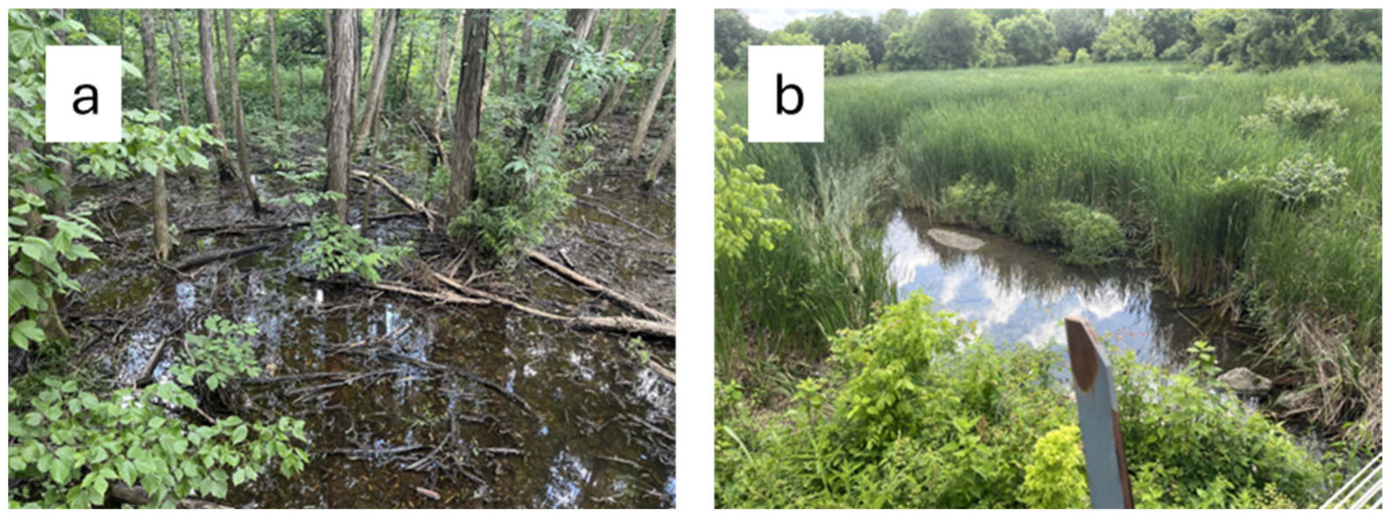
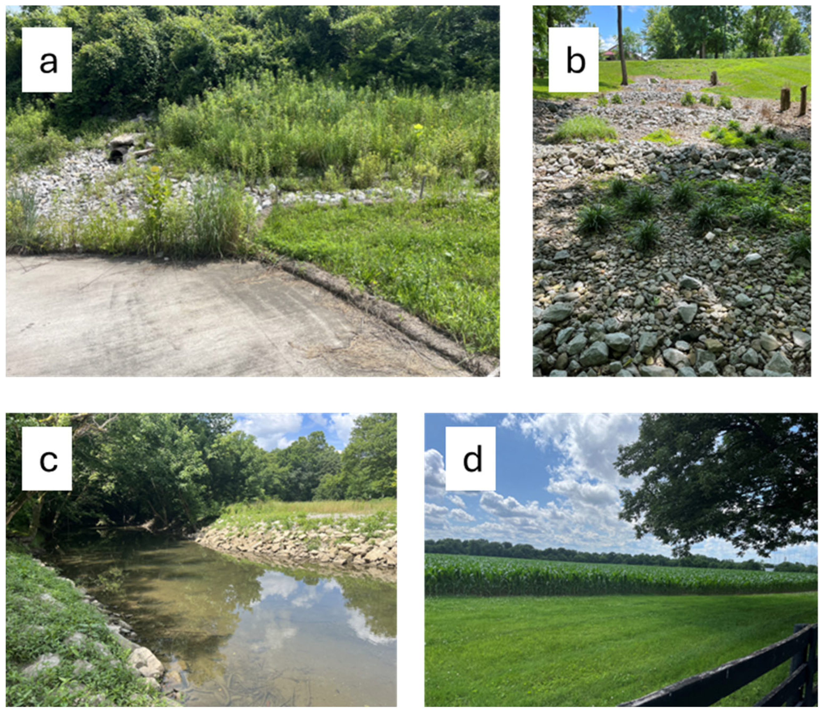
In addition to distributed within-reach sediment sources, reconstructed wetlands located directly upstream of the Up gauge (Figure 12) may also influence turbidity dynamics by modifying sediment supply entering the monitored reach. Such features can reduce flow velocities, promote temporary sediment storage, and dampen extreme turbidity peaks during longer, lower-energy storm events, thereby conditioning the upstream turbidity signal that propagates downstream [89,90]. By moderating sediment delivery to the channel network upstream of the gauge, these wetlands may contribute to the more uniform upstream–downstream turbidity relationships and near-unity turbidity ratios observed during many winter and spring storms, when local sediment sources are less active.

These patterns are also consistent with geomorphic characteristics common in many urban stream systems, where channel incision, bank instability, and exposed bed sediments create abundant near-channel sediment sources [2]. During high-intensity storms, rapid runoff generated from impervious surfaces can mobilize these materials quickly, producing localized turbidity pulses that are partially decoupled from upstream sediment inputs. Such dynamics are consistent with conceptual models of urban sediment transport in which altered channel morphology and stormwater infrastructure increase connectivity between sediment sources and the channel network during high-energy runoff events. Although impervious surfaces in urban areas reduce the potential for direct rainfall-driven soil detachment from hillslopes, they also increase runoff generation and flow velocity during storm events. These changes can enhance channel erosion and mobilization of stored sediments within the stream network. As a result, sediment transport in urban watersheds is often dominated by in-channel sources rather than hillslope erosion, particularly during high-intensity storms when hydraulic connectivity increases.

4.3. Event-Scale Sediment Timing and Hysteresis Behavior

The hysteresis results provide an additional line of evidence supporting the seasonal patterns observed in both the regression and turbidity-ratio analyses. The consistent clockwise hysteresis exhibited across all events indicates that turbidity generally rose and peaked prior to discharge, reflecting rapid sediment mobilization at the onset of storms [45,70]. This pattern is widely documented in small and urbanizing catchments where fine sediment stored in channels, hillslopes, or near-channel sources is quickly entrained by the initial runoff pulse before discharge has fully developed [44]. The dominance of clockwise loops across all seasons suggests that the watershed contains readily mobilizable sediment sources near the channel network, a condition consistent with the reach-scale sediment connectivity inferred from the winter and spring turbidity ratios.

In urban streams, in-channel sediment sources such as eroding banks, exposed bed sediments, and previously deposited fine material can also contribute to early turbidity peaks and influence hysteresis patterns. Storm runoff can rapidly entrain these readily available sediments during the initial rise in the hydrograph, producing turbidity responses that precede peak discharge and reinforcing clockwise hysteresis behavior. Similar mechanisms have been documented in urban and headwater systems where bank erosion and near-channel sediment storage provide readily mobilized sediment during storm events [44,69,70].

The larger loop areas and more extreme negative peak lags observed in summer and, to a lesser extent, fall events indicate more abrupt and spatially heterogeneous sediment activation during these storms. Pronounced temporal offsets between turbidity and discharge peaks reflect rapid mobilization of localized sediment sources and limited temporal integration of sediment signals across the watershed, a behavior commonly associated with event-scale sediment hysteresis under highly episodic runoff conditions [38,91]. This pattern reinforces the regression results showing weaker and more variable lagged relationships during warm-season storms and is consistent with the turbidity-ratio evidence pointing to substantial within-reach sediment contributions during these events.

In contrast, winter and spring events exhibited smaller hysteresis magnitudes and reduced timing offsets between turbidity and discharge peaks. Sustained wet-season precipitation increases antecedent moisture and hydrologic connectivity, promoting more synchronized turbidity and discharge responses and producing smaller, more coherent hysteresis loops [92,93]. These hysteresis characteristics are consistent with the strong and statistically stable upstream–downstream turbidity relationships identified by the regression models during cool-season storms.

Overall, the hysteresis analysis complements the regression and turbidity-ratio findings by demonstrating that storm structure governs not only the magnitude and spatial origin of turbidity but also its temporal alignment with discharge. These results underscore that seasonal shifts in rainfall type, storm duration, sediment connectivity, and antecedent moisture collectively shape the form and strength of turbidity–discharge hysteresis, reinforcing the need for storm-type-specific approaches when modeling or interpreting sediment dynamics in nested watershed systems.

4.4. Implications for Sediment Best Management Practice (BMP) Design

Because turbidity in this study reflects storm-driven mobilization and transport of fine sediment, management implications are framed in terms of sediment control. The Middle Fork Beargrass Creek Watershed-Based Plan also identifies both sediment and turbidity as priority water quality concerns, noting that nonpoint source runoff from highly impervious surfaces (estimated at 37% of the watershed in the plan) combined with historical channelization contributes to elevated suspended sediment levels and declining habitat conditions [41]. The plan further emphasizes the need for integrated structural and nonstructural management approaches, providing relevant context for our findings. Our results indicate that storm seasonality, sediment source connectivity, and event timing should be considered when evaluating the effectiveness of best management practices (BMPs) for turbidity and sediment control in urban watersheds.

Downstream turbidity in the Middle Fork of Beargrass Creek did not respond uniformly to storm forcing, instead reflecting seasonally varying interactions among upstream sediment transport, localized sediment generation, and storm morphology. Similar seasonal variability in urban water-quality responses has been documented in other watersheds, where the magnitude and direction of urban impacts vary throughout the year [94]. Winter and spring storms were generally longer in duration and exhibited stronger upstream–downstream turbidity coherence and more stable lag relationships. During these seasons, turbidity ratios were closer to unity, and hysteresis loops showed smaller normalized areas, indicating more integrated sediment transport across the watershed. Under such conditions, BMPs that attenuate runoff volumes, extend flow paths, and enhance sediment retention—such as floodplain reconnection, riparian buffers and wetlands, and detention or retention basins—are likely to be particularly effective. Similar findings have been reported in mixed land-use and water-supply watersheds, where sustained, lower-intensity storms promote coherent sediment routing and improve the performance of watershed-scale sediment controls [95].

The watershed currently contains 64 local detention basins that provide sediment settling during storm events, and the watershed plan noted that while these existing facilities play an important role, opportunities exist to enhance their effectiveness through retrofits and strategic placement of additional facilities [41]. In Louisville, MSD regulations require post-construction water-quality BMPs (e.g., bioretention, wet/dry basins, vegetated buffers) for permitted development, reflecting this emphasis on runoff attenuation and sediment storage [96]. Additionally, reconstructed wetlands located upstream of the Up gauge (Figure 12) may contribute to the more uniform upstream–downstream turbidity relationships observed during winter and spring storms by moderating sediment delivery, reducing flow velocities, and dampening extreme turbidity peaks during longer, lower-energy storm events [89,90]. At the state level, additional guidance and technical resources for erosion prevention and sediment management are provided through Kentucky’s nonpoint source program [97].

In contrast, summer and fall storms were typically shorter in duration but higher in intensity and erosivity, producing elevated turbidity ratios and pronounced clockwise hysteresis indicative of rapid, localized sediment mobilization. Regression models for these events showed weaker and more variable lag relationships, suggesting that downstream turbidity was often decoupled from upstream conditions and dominated by within-reach or near-channel sediment sources contributing to downstream turbidity (Figure 13). This behavior is consistent with observations from other urban watersheds, where high-intensity convective storms preferentially activate sediment sources associated with eroding streambanks, road networks, and construction activity rather than upstream sediment supply [69,80]. The watershed plan also identifies critical sediment sources requiring targeted stabilization, documenting bank instability, vertical banks, and embedded stream substrates [41], conditions that our results suggest are most problematic during high-intensity warm-season storms.

Under these warm-season conditions, BMPs that focus primarily on upstream runoff attenuation may have limited effectiveness for reducing downstream turbidity. Instead, practices that stabilize local sediment sources and intercept sediment close to points of mobilization become increasingly important. These include enhanced erosion and sediment controls at construction sites, bioengineered streambank stabilization, vegetated swales, and decentralized green infrastructure that reduces directly connected impervious areas (Figure 14). The watershed plan emphasizes streambank stabilization and erosion control as critical structural BMPs, alongside nonstructural measures including improved street sweeping to remove accumulated fine sediment from impervious surfaces and routine maintenance of stormwater conveyance systems to prevent sediment re-mobilization [41].

Wider analyses of urban streams similarly show that turbidity is often more strongly influenced by site-scale factors—such as riparian vegetation, land disturbance, and streambank stability—than by aggregate measures of watershed urbanization, underscoring the importance of localized BMP implementation [80,84,98]. The consistent dominance of clockwise hysteresis across all seasons further reinforces this finding, indicating rapid entrainment of fine sediment early in storm events—a pattern widely observed in urban, mixed land-use, and regulated river systems [80,99]. This source control emphasis aligns with local watershed approaches such as Louisville’s Healthy Watershed Initiative, which supports watershed planning, pollution reduction, and BMP demonstration projects [100].

Local stormwater management programs provide further practical examples of how these principles can be implemented. Federal guidance emphasizes combining source control measures, land-use planning, and structural BMPs to reduce sediment and contaminant delivery during storm events, particularly in urban watersheds with flashy hydrologic responses [101]. In Jefferson County, post-construction BMP requirements—including bioretention, green infrastructure, vegetated buffers, and stormwater basins—are codified through MSD’s erosion prevention and sediment control regulations [102]. The findings of this study support these approaches while also highlighting the importance of seasonal context: volume- and connectivity-based BMPs are likely to be most effective during winter and spring, whereas source control and stabilization measures are critical during summer and fall when turbidity responses are more localized and episodic.

Taken together, these results suggest that BMP planning in urban watersheds may benefit from moving beyond uniform design standards toward adaptive strategies that account for storm seasonality, sediment source location, and event timing. Aligning BMP type and placement with dominant sediment transport processes operating under different storm regimes is increasingly recognized as essential for effective turbidity reduction and source-water protection [95] and is consistent with statewide watershed planning frameworks in Kentucky that emphasize integrated, cross-agency approaches to water-quality management. The seasonal patterns and sediment source dynamics identified in this study can directly inform implementation of the Middle Fork Beargrass Creek Watershed-Based Plan [41] by helping to prioritize BMP types and locations based on dominant storm characteristics and expected sediment transport pathways throughout the year. Specifically, our findings support the plan’s dual emphasis on watershed-scale detention and connectivity improvements for cool-season conditions, and targeted source controls and streambank stabilization for warm-season conditions when localized sediment mobilization dominates turbidity responses.

4.5. Directions for Future Research

The event-scale framework applied in this study highlights several avenues for future research that could further advance understanding of turbidity and sediment dynamics in urban watersheds. Extending this approach to additional watersheds with contrasting land-use patterns, channel morphologies, and stormwater infrastructure would allow assessment of the generality of the seasonal and spatial controls identified here. Longer monitoring records would also enable evaluation of interannual variability and the influence of extreme events, which are expected to become more frequent under changing climate conditions.

Future work could also focus on more explicitly characterizing sediment sources and storage within urban stream networks. While turbidity ratios, lag sensitivity, and hysteresis patterns provide strong indirect evidence of within-reach sediment contributions, integrating complementary datasets—such as reach-scale geomorphic surveys, bank erosion monitoring, sediment fingerprinting, or high-resolution construction and land-disturbance records—would enable more direct attribution of sediment sources and pathways. Such integration would strengthen inference regarding the relative importance of upstream transport versus local sediment mobilization during different storm regimes.

In addition, targeted investigation of engineered features within the watershed, including stormwater infrastructure and constructed or restored wetlands, could improve understanding of how these elements modify sediment routing and timing during storm events. Monitoring upstream and downstream of individual features during storms would help quantify their role in sediment storage, release, and attenuation, providing valuable information for both modeling efforts and BMP design.

Finally, the variability observed during short-duration, high-intensity storms suggests opportunities to refine event-based modeling approaches. Future studies could explore storm-type classification, non-linear or threshold-based models, or hybrid approaches that combine hydrometeorological drivers with indicators of sediment availability. Such efforts would be particularly useful for capturing rapid and spatially heterogeneous turbidity responses that are less well represented by linear lagged frameworks. Together, these research directions build directly on the findings of this study and offer pathways for improving both scientific understanding and management of storm-driven turbidity in urban stream systems.

5. Conclusions

This study examined seasonal controls on storm-driven turbidity dynamics in an urban watershed using high-resolution monitoring data from the Middle Fork of Beargrass Creek, Louisville, Kentucky. The key findings include:

• Seasonal storm structure strongly influenced turbidity predictability. Winter and spring storms, characterized by longer durations and lower intensities, produced stronger upstream–downstream turbidity coupling and more stable regression relationships (mean R² = 0.85 and 0.74, respectively). Summer storms, despite higher erosivity, exhibited shorter durations, weaker predictive relationships (mean R² = 0.68), and greater model sensitivity to lag specification.
• Sediment source contributions varied seasonally. Turbidity ratios approached unity during winter and spring, indicating integrated sediment transport from upstream sources. In contrast, summer and fall events produced elevated ratios (up to 75.5), reflecting localized sediment mobilization within the downstream reach independent of upstream conditions. These results further suggest that localized sediment sources within the urban channel network, including eroding banks and exposed bed sediments, may play an important role in shaping turbidity responses during storm events, particularly during high-intensity rainfall when runoff connectivity increases.
• Clockwise hysteresis dominated across all seasons. Turbidity consistently peaked before discharge, indicating rapid mobilization of near-channel sediment sources. However, summer and fall storms exhibited larger hysteresis loop areas and earlier turbidity peaks, consistent with episodic activation of local sediment stores.
• Lagged upstream turbidity was the dominant predictor of downstream turbidity. Standardized regression coefficients for lagged upstream turbidity ranged from 0.70 to 0.90 across seasons, while lagged downstream erosivity showed greater seasonal variability (0.14 to 0.41), with the strongest effects during high-intensity summer storms. This further reflects the mobilization of sediments from multiple sources, including channel erosion, stored sediments, and stormwater runoff pathways.
• BMP effectiveness likely varies by season and storm type. Results suggest that volume-reduction and connectivity-based BMPs (e.g., detention basins, riparian buffers, wetlands) may be most effective during winter and spring, while source control measures (e.g., streambank stabilization, construction site controls, street sweeping) are critical during summer and fall when turbidity responses are driven by localized sediment mobilization.

These findings demonstrate that seasonally adaptive approaches to turbidity monitoring, modeling, and management are essential in urban watersheds where storm characteristics and sediment transport pathways vary throughout the year. Future research could further improve understanding of storm-driven turbidity dynamics in urban watersheds by integrating high-frequency monitoring with sediment source identification techniques, such as sediment fingerprinting or geomorphic assessments of channel erosion. Expanding monitoring networks to include additional upstream tributaries and stormwater outfalls would also help clarify how urban drainage infrastructure influences sediment transport pathways and turbidity responses during storm events.

References

1. Zarnaghsh, A.; Husic, A. An index for inferring dominant transport pathways of solutes and sediment: Assessing land use impacts with high-frequency conductivity and turbidity sensor data. Sci. Total Environ. 2023, 894, 164931. [Google Scholar] [CrossRef] [PubMed]
2. Walsh, C.J.; Roy, A.H.; Feminella, J.W.; Cottingham, P.D.; Groffman, P.M.; Morgan, R.P. The urban stream syndrome: Current knowledge and the search for a cure. J. N. Am. Benthol. Soc. 2005, 24, 706–723. [Google Scholar] [CrossRef]
3. Booth, D.B.; Hartley, D.; Jackson, R. Forest cover, impervious-surface area, and the mitigation of stormwater impacts. J. Am. Water Resour. Assoc. 2002, 38, 835–845. [Google Scholar] [CrossRef]
4. Zhang, J.; Li, Z.; Li, X.; Zhang, L.; Duan, D. Impact of land use changes on total rainfall and urban hydrological fluxes. Geomat. Nat. Hazards Risk 2025, 16, 2545387. [Google Scholar] [CrossRef]
5. Brown, L.R.; Cuffney, T.F.; Coles, J.F.; Fitzpatrick, F.; McMahon, G.; Steuer, J.; Bell, A.H.; May, J.T. Urban streams across the USA: Lessons learned from studies in 9 metropolitan areas. J. N. Am. Benthol. Soc. 2009, 28, 1051–1069. [Google Scholar] [CrossRef]
6. Rasmussen, P.P.; Gray, J.R.; Glysson, G.D.; Ziegler, A.C. Guidelines and Procedures for Computing Time-Series Suspended-Sediment Concentrations and Loads from In-Stream Turbidity-Sensor and Streamflow Data. In US Geological Survey Techniques and Methods 3-C4; U.S. Geological Survey: Reston, VA, USA, 2009. [Google Scholar] [CrossRef]
7. McGrane, S.J. Impacts of urbanisation on hydrological and water quality dynamics, and urban water management: A review. Hydrol. Sci. J. 2016, 61, 2295–2311. [Google Scholar] [CrossRef]
8. Ellis, J.B.; Mitchell, G. Urban diffuse pollution: Key data information approaches for the Water Framework Directive. Water Environ. J. 2006, 20, 19–26. [Google Scholar] [CrossRef]
9. MacKenzie, K.M.; Singh, K.; Binns, A.D.; Whiteley, H.R.; Gharabaghi, B. Effects of urbanization on stream flow, sediment, and phosphorous regime. J. Hydrol. 2022, 612, 128283. [Google Scholar] [CrossRef]
10. Porter, A. Stormwater Quantity and Quality in Selected Urban Watersheds in Hampton Roads, Virginia, 2016–2020; US Geological Survey Scientific Investigations Report 2022-511; U.S. Geological Survey: Reston, VA, USA, 2022. [CrossRef]
11. Wang, S.; He, Q.; Ai, H.; Wang, Z.; Zhang, Q. Pollutant concentrations and pollution loads in stormwater runoff from different land uses in Chongqing. J. Environ. Sci. 2013, 25, 502–510. [Google Scholar] [CrossRef]
12. Steffy, L.Y.; Shank, M.K. Considerations for using turbidity as a surrogate for suspended sediment in small, ungaged streams: Time-series selection, streamflow estimation, and regional transferability. River Res. Appl. 2018, 34, 1304–1314. [Google Scholar] [CrossRef]
13. Müller, A.; Österlund, H.; Marsalek, J.; Viklander, M. The pollution conveyed by urban runoff: A review of sources. Sci. Total Environ. 2020, 709, 136125. [Google Scholar] [CrossRef]
14. Walch, H.; Von Der Kammer, F.; Hofmann, T. Freshwater suspended particulate matter—Key components and processes in floc formation and dynamics. Water Res. 2022, 220, 118655. [Google Scholar] [CrossRef]
15. Lenhart, C.F.; Brooks, K.N.; Heneley, D.; Magner, J.A. Spatial and temporal variation in suspended sediment, organic matter, and turbidity in a Minnesota prairie river: Implications for TMDLs. Environ. Monit. Assess. 2010, 165, 435–447. [Google Scholar] [CrossRef]
16. Yin, S.; Xie, Y.; Liu, B.; Nearing, M.A. Rainfall erosivity estimation based on rainfall data collected over a range of temporal resolutions. Hydrol. Earth Syst. Sci. 2015, 19, 4113–4126. [Google Scholar] [CrossRef]
17. Ahilan, S.; Guan, M.; Sleigh, A.; Wright, N.; Chang, H. The influence of floodplain restoration on flow and sediment dynamics in an urban river. J. Flood Risk Manag. 2018, 11, S986–S1001. [Google Scholar] [CrossRef]
18. Lewis, J. Turbidity-controlled suspended sediment sampling for runoff-event load estimation. Water Resour. Res. 1996, 32, 2299–2310. [Google Scholar] [CrossRef]
19. Bilotta, G.S.; Brazier, R.E. Understanding the influence of suspended solids on water quality and aquatic biota. Water Res. 2008, 42, 2849–2861. [Google Scholar] [CrossRef]
20. McHale, M.R.; Siemion, J. Turbidity and Suspended Sediment in the Upper Esopus Creek Watershed, Ulster County, New York; US Geological Survey Scientific Investigations Report 2014-5200; U.S. Geological Survey: Reston, VA, USA, 2014. [CrossRef]
21. Walsh, C.J.; Fletcher, T.D.; Burns, M.J. Urban stormwater runoff: A new class of environmental flow problem. PLoS ONE 2012, 7, e45814. [Google Scholar] [CrossRef]
22. Gaffield, S.J.; Goo, R.L.; Richards, L.A.; Jackson, R.J. Public health effects of inadequately managed stormwater runoff. Am. J. Public Health 2003, 93, 1527–1533. [Google Scholar] [CrossRef]
23. Blaszczak, J.R.; Delesantro, J.M.; Urban, D.L.; Doyle, M.W.; Bernhardt, E.S. Scoured or suffocated: Urban stream ecosystems oscillate between hydrologic and dissolved oxygen extremes. Limnol. Oceanogr. 2019, 64, 877–894. [Google Scholar] [CrossRef]
24. Drummond, J.D.; Larsen, L.G.; González-Pinzón, R.; Packman, A.I.; Harvey, J.W. Less fine particle retention in a restored versus unrestored urban stream: Balance between hyporheic exchange, resuspension, and immobilization. JGR Biogeosci. 2018, 123, 1425–1439. [Google Scholar] [CrossRef]
25. Katz, S.B.; Segura, C.; Warren, D.R. The influence of channel bed disturbance on benthic Chlorophyll a: A high resolution perspective. Geomorphology 2018, 305, 141–153. [Google Scholar] [CrossRef]
26. Almeida, W.S.D.; Seitz, S.; Oliveira, L.F.C.D.; Carvalho, D.F.D. Duration and intensity of rainfall events with the same erosivity change sediment yield and runoff rates. Int. Soil Water Conserv. Res. 2021, 9, 69–75. [Google Scholar] [CrossRef]
27. Day, C.A.; Liebman, J. Modeling seasonal sediment yields for a medium-scale temperate forest/agricultural watershed. Phys. Geogr. 2022, 43, 829–852. [Google Scholar] [CrossRef]
28. Day, C.A.; Long, Q.A. A GIS-based approach for estimating fallow-season cropland soil erosion based on rainfall erosivity. Phys. Geogr. 2023, 44, 763–781. [Google Scholar] [CrossRef]
29. Nearing, M.A.; Yin, S.; Borrelli, P.; Polyakov, V.O. Rainfall erosivity: An historical review. Catena 2017, 157, 357–362. [Google Scholar] [CrossRef]
30. Yin, S.; Nearing, M.A.; Borrelli, P.; Xue, X. Rainfall erosivity: An overview of methodologies and applications. Vadose Zone J. 2017, 16, 1–16. [Google Scholar] [CrossRef]
31. Kinnell, P.I.A. Indices accounting for rainstorm erosivity—Theory and practice. Catena 2023, 223, 106925. [Google Scholar] [CrossRef]
32. Russell, K.L.; Vietz, G.J.; Fletcher, T.D. Urban sediment supply to streams from hillslope sources. Sci. Total Environ. 2019, 653, 684–697. [Google Scholar] [CrossRef]
33. Ferdowsi, A.; Piadeh, F.; Behzadian, K.; Mousavi, S.F.; Ehteram, M. Urban water infrastructure: A critical review on climate change impacts and adaptation strategies. Urban Clim. 2024, 58, 102132. [Google Scholar] [CrossRef]
34. Melillo, J.M.; Richmond, T.C.; Yohe, G.W. Climate Change Impacts in the United States. US National Climate Assessment; US Global Change Research Program: Washington, DC, USA, 2014. [CrossRef]
35. Myhre, G.; Alterskjær, K.; Stjern, C.W.; Hodnebrog, Ø.; Marelle, L.; Samset, B.H.; Sillmann, J.; Schaller, N.; Fischer, E.; Schulz, M.; et al. Frequency of extreme precipitation increases extensively with event rareness under global warming. Sci. Rep. 2019, 9, 16063. [Google Scholar] [CrossRef]
36. Kim, J.; Porter, J.; Kearns, E.J. Exposure of the US population to extreme precipitation risk has increased due to climate change. Sci. Rep. 2023, 13, 21782. [Google Scholar] [CrossRef]
37. García, J.T.; Harrington, J.R. Fine sediment modeling during storm-based events in the River Bandon, Ireland. Water 2019, 11, 1523. [Google Scholar] [CrossRef]
38. Wymore, A.S.; Leon, M.C.; Shanley, J.B.; McDowell, W.H. Hysteretic response of solutes and turbidity at the event scale across forested tropical montane watersheds. Front. Earth Sci. 2019, 7, 126. [Google Scholar] [CrossRef]
39. Hawley, R.J.; Russell, K.; Taniguchi-Quan, K. Restoring geomorphic integrity in urban streams via mechanistically-based storm water management: Minimizing excess sediment transport capacity. Urban Ecosyst. 2022, 25, 1247–1264. [Google Scholar] [CrossRef]
40. Andualem, T.G.; Hewa, G.A.; Myers, B.R.; Boland, J.; Peters, S. Predicting suspended sediment transport in urbanised streams: A case study of Dry Creek, South Australia. Hydrology 2024, 11, 196. [Google Scholar] [CrossRef]
41. Metropolitan Sewer District (MSD). Middle Fork Beargrass Creek Watershed-Based Plan. 2022. Available online: https://louisvillemsd.org/sites/default/files/file_repository/HealthyWatershed/Middle%20Fork%20Beargrass%20Creek%20Watershed%20Based%20Plan.pdf (accessed on 30 March 2026).
42. Hawley, R.J.; Korth, N.L.; Olinde, L.J. Designing stormwater controls to protect streams from erosion—A simple (and implementable) channel-protection strategy. Freshw. Sci. 2025, 44, 463–474. [Google Scholar] [CrossRef]
43. Renard, K.; Foster, G.; Weesies, G.; McCool, D.; Yoder, D. Predicting Soil Erosion by Water: A Guide to Conservation Planning with the Revised Universal Soil Loss Equation (RUSLE); Agriculture Handbook No.703; US Department of Agriculture: Washington, DC, USA, 1997.
44. Smith, H.G.; Dragovich, D. Interpreting sediment delivery processes using suspended sediment-discharge hysteresis patterns from nested upland catchments, south-eastern Australia. Hydrol. Process. 2009, 23, 2415–2426. [Google Scholar] [CrossRef]
45. Lloyd, C.E.M.; Freer, J.E.; Johnes, P.J.; Collins, A.L. Technical Note: Testing an improved index for analysing storm discharge–concentration hysteresis. Hydrol. Earth Syst. Sci. 2016, 20, 625–632. [Google Scholar] [CrossRef]
46. R Foundation. The R Project for Statistical Computing. 2025. Available online: https://www.r-project.org/ (accessed on 24 January 2026).
47. Kentucky Farm Bureau. Only by the Grace of God. 2025. Available online: https://www.kyfb.com/federation/newsroom/only-by-the-grace-of-god/ (accessed on 24 January 2026).
48. US Geological Survey. Annual NLCD Collection 1 Science Products; U.S. Geological Survey: Reston, VA, USA, 2024. [CrossRef]
49. NOAANWS Climatology—Louisville. 2026. Available online: https://www.weather.gov/lmk/clisdf (accessed on 24 January 2026).
50. Jarrett, L.G.; Downs, A.C.; Grace-Jarrett, P.A. Continuous Hydrologic Simulation of Runoff for the Middle Fork and South Fork of the Beargrass Creek Basin in Jefferson County, Kentucky; Water-Resources Investigations Report 98-4182; US Geological Survey: Reston, VA, USA, 1998.
51. Metropolitan Sewer District (MSD). Louisville MSD Rain Gauge. 2025. Available online: https://raingauge.louisvillemsd.org/RainGauge.aspx (accessed on 24 January 2026).
52. Wischmeier, W.H.; Smith, D.D. Predicting Rainfall Erosion Losses—A Guide to Conservation Planning; Agriculture Handbook No. 537; US Department of Agriculture: Washington, DC, USA, 1978.
53. Beven, K.J. Rainfall-Runoff Modelling: The Primer, 2nd ed.; Wiley-Blackwell: Hoboken, NJ, USA, 2012. [Google Scholar]
54. Joo, J.; Lee, J.; Kim, J.; Jun, H.; Jo, D. Inter-event time definition setting procedure for urban drainage systems. Water 2013, 6, 45–58. [Google Scholar] [CrossRef]
55. Tu, A.; Zeng, J.; Liu, Z.; Zheng, H.; Xie, S. Effect of minimum inter-event time for rainfall event separation on rainfall properties and rainfall erosivity in a humid area of southern China. Geoderma 2023, 431, 116332. [Google Scholar] [CrossRef]
56. Helsel, D.R.; Hirsch, R.M.; Ryberg, K.R.; Archfield, S.A.; Gilroy, E.J. Statistical Methods in Water Resources. In US Geological Survey Techniques and Methods 4-A3; U.S. Geological Survey: Reston, VA, USA, 2020. [Google Scholar] [CrossRef]
57. US Geological Survey. National Water Dashboard. 2025. Available online: https://dashboard.waterdata.usgs.gov/app/nwd/en/ (accessed on 24 January 2026).
58. Alexander, J.S.; Girard, C.; Campbell, J.; Ellison, C.; Gosselin, E.; Smith, E. Using Continuous Measurements of Turbidity to Predict Suspended-Sediment Concentrations, Loads, and Sources in Flat Creek Through the Town of Jackson, Wyoming, 2019−20—A Pilot Study; US Geological Survey Open-File Report 2022-1103; U.S. Geological Survey: Reston, VA, USA, 2022. [CrossRef]
59. Chow, V.T. Open Channel Hydraulics; McGraw-Hill: Columbus, OH, USA, 1959. [Google Scholar]
60. Natural Resources Conservation Service (NRCS). Chapter 15: Time of Concentration. In Part 630 Hydrology National Engineering Handbook; Natural Resources Conservation Service: Washington, DC, USA, 2010. [Google Scholar]
61. Nearing, M.; Jetten, V.; Baffaut, C.; Cerdan, O.; Couturier, A.; Hernandez, M.; Le Bissonnais, Y.; Nichols, M.; Nunes, J.; Renschler, C.; et al. Modeling response of soil erosion and runoff to changes in precipitation and cover. Catena 2005, 61, 131–154. [Google Scholar] [CrossRef]
62. Uhrich, M.; Kolasinac, J.; Booth, P.; Fountain, R.; Spicer, K.; Mosbrucker, A.R. Correlations of Turbidity to Suspended-Sediment Concentration in the Toutle River Basin, near Mount St. Helens, Washington, 2010–2011; US Geological Survey Open-File Report 2014-1204; US Geological Survey: Reston, VA, USA, 2014. [CrossRef][Green Version]
63. Zeileis, A. Econometric computing with HC and HAC covariance matrix estimators. J. Stat. Softw. 2004, 11, 1–17. [Google Scholar] [CrossRef]
64. Passerotti, G.; Massazza, G.; Pezzoli, A.; Bigi, V.; Zsótér, E.; Rosso, M. Hydrological model application in the Sirba River: Early warning system and GloFAS improvements. Water 2020, 12, 620. [Google Scholar] [CrossRef]
65. Gao, P.; Josefson, M. Temporal variations of suspended sediment transport in Oneida Creek watershed, central New York. J. Hydrol. 2012, 426–427, 17–27. [Google Scholar] [CrossRef]
66. Gellis, A.C.; Noe, G.B. Sediment source analysis in the Linganore Creek watershed, Maryland, USA, using the sediment fingerprinting approach: 2008 to 2010. J. Soils Sediments 2013, 13, 1735–1753. [Google Scholar] [CrossRef]
67. Vercruysse, K.; Grabowski, R.C.; Rickson, R.J. Suspended sediment transport dynamics in rivers: Multi-scale drivers of temporal variation. Earth-Sci. Rev. 2017, 166, 38–52. [Google Scholar] [CrossRef]
68. Jing, T.; Zeng, Y.; Fang, N.; Dai, W.; Shi, Z. A review of suspended sediment hysteresis. Water Resour. Res. 2025, 61, e2024WR037216. [Google Scholar] [CrossRef]
69. Lawler, D.M.; Petts, G.E.; Foster, I.D.L.; Harper, S. Turbidity dynamics during spring storm events in an urban headwater river system: The Upper Tame, West Midlands, UK. Sci. Total Environ. 2006, 360, 109–126. [Google Scholar] [CrossRef]
70. Lloyd, C.E.M.; Freer, J.E.; Johnes, P.J.; Collins, A.L. Using hysteresis analysis of high-resolution water quality monitoring data, including uncertainty, to infer controls on nutrient and sediment transfer in catchments. Sci. Total Environ. 2016, 543, 388–404. [Google Scholar] [CrossRef]
71. Zuecco, G.; Penna, D.; Borga, M.; Van Meerveld, H.J. A versatile index to characterize hysteresis between hydrological variables at the runoff event timescale. Hydrol. Process. 2016, 30, 1449–1466. [Google Scholar] [CrossRef]
72. Beven, K.; Binley, A. The future of distributed models: Model calibration and uncertainty prediction. Hydrol. Process. 1992, 6, 279–298. [Google Scholar] [CrossRef]
73. Gupta, H.V.; Sorooshian, S.; Yapo, P.O. Toward improved calibration of hydrologic models: Multiple and noncommensurable measures of information. Water Resour. Res. 1998, 34, 751–763. [Google Scholar] [CrossRef]
74. Krause, P.; Boyle, D.P.; Bäse, F. Comparison of different efficiency criteria for hydrological model assessment. Adv. Geosci. 2005, 5, 89–97. [Google Scholar] [CrossRef]
75. Moriasi, D.N.; Arnold, J.G.; Van Liew, M.W.; Bingner, R.L.; Harmel, R.D.; Veith, T.L. Model evaluation guidelines for systematic quantification of accuracy in watershed simulations. Trans. ASABE 2007, 50, 885–900. [Google Scholar] [CrossRef]
76. Tye, A.M.; Leeming, K.A.; Gong, M.; Marchant, B.; Hurst, M.D. Assessment of suspended sediment export and dynamics using in-line turbidity sensors and time series statistical models. Earth Surf. Process. Landf. 2024, 49, 4113–4132. [Google Scholar] [CrossRef]
77. Istanbulluoglu, E.; Tarboton, D.G.; Pack, R.T.; Luce, C.H. Modeling of the interactions between forest vegetation, disturbances, and sediment yields. J. Geophys. Res. 2004, 109, 2003JF000041. [Google Scholar] [CrossRef]
78. Qian, J.L.; Wu, Y.X.; Zhang, Q.T. The response of small watershed storm floods to climate change. Water 2024, 17, 33. [Google Scholar] [CrossRef]
79. Göransson, G.; Larson, M.; Bendz, D. Variation in turbidity with precipitation and flow in a regulated river system—River Göta Älv, SW Sweden. Hydrol. Earth Syst. Sci. 2013, 17, 2529–2542. [Google Scholar] [CrossRef]
80. Safdar, S.; Jefferson, A.J.; Costello, D.M.; Blinn, A. Urbanization and suspended sediment transport dynamics: A comparative study of watersheds with varying degree of urbanization using concentration-discharge hysteresis. ACS EST Water 2024, 4, 3904–3917. [Google Scholar] [CrossRef]
81. Liu, W.; Birgand, F.; Tian, S.; Chen, C. Event-scale hysteresis metrics to reveal processes and mechanisms controlling constituent export from watersheds: A review. Water Res. 2021, 200, 117254. [Google Scholar] [CrossRef]
82. Montgomery, D.R.; Buffington, J.M. Chapter 2: Channel processes, classification and response. In River Ecology and Management: Lessons from the Pacific Coastal Ecoregion, 1st ed.; Naiman, R.J., Bilby, R.E., Eds.; Springer: Berlin/Heidelberg, Germany, 2001; pp. 13–42. [Google Scholar]
83. Gomi, T.; Sidle, R.C.; Richardson, J.S. Understanding processes and downstream linkages of headwater systems. BioScience 2002, 52, 905–916. [Google Scholar] [CrossRef]
84. Malhotra, K.; Lamba, J.; Shepherd, S. Sources of stream bed sediment in an urbanized watershed. Catena 2020, 184, 104228. [Google Scholar] [CrossRef]
85. Ali, G.A.; Roy, A.G. Shopping for hydrologically representative connectivity metrics in a humid temperate forested catchment. Water Resour. Res. 2010, 46, 2010WR009442. [Google Scholar] [CrossRef]
86. Zimmer, M.A.; McGlynn, B.L. Ephemeral and intermittent runoff generation processes in a low relief, highly weathered catchment. Water Resour. Res. 2017, 53, 7055–7077. [Google Scholar] [CrossRef]
87. Bracken, L.J.; Croke, J. The concept of hydrological connectivity and its contribution to understanding runoff-dominated geomorphic systems. Hydrol. Process. 2007, 21, 1749–1763. [Google Scholar] [CrossRef]
88. Wohl, E.; Brierley, G.; Cadol, D.; Coulthard, T.J.; Covino, T.; Fryirs, K.A.; Grant, G.; Hilton, R.G.; Lane, S.N.; Magilligan, F.J.; et al. Connectivity as an emergent property of geomorphic systems. Earth Surf. Process. Landf. 2019, 44, 4–26. [Google Scholar] [CrossRef]
89. Kadlec, R.H.; Wallace, S.D. Treatment Wetlands, 2nd ed.; CRC Press: Boca Raton, FL, USA, 2009. [Google Scholar]
90. Mitsch, W.J.; Zhang, L.; Stefanik, K.C.; Nahlik, A.M.; Anderson, C.J.; Bernal, B.; Hernandez, M.; Song, K. Creating wetlands: Primary succession, water quality changes, and self-design over 15 years. BioScience 2012, 62, 237–250. [Google Scholar] [CrossRef]
91. Seeger, M.; Errea, M.-P.; Beguería, S.; Arnáez, J.; Martí, C.; García-Ruiz, J. Catchment soil moisture and rainfall characteristics as determinant factors for discharge/suspended sediment hysteretic loops in a small headwater catchment in the Spanish Pyrenees. J. Hydrol. 2004, 288, 299–311. [Google Scholar] [CrossRef]
92. Mano, V.; Nemery, J.; Belleudy, P.; Poirel, A. Assessment of suspended sediment transport in four alpine watersheds (France): Influence of the climatic regime. Hydrol. Process. 2009, 23, 777–792. [Google Scholar] [CrossRef]
93. López-Tarazón, J.A.; Batalla, R.J.; Vericat, D.; Francke, T. The sediment budget of a highly dynamic mesoscale catchment: The River Isábena. Geomorphology 2012, 138, 15–28. [Google Scholar] [CrossRef]
94. Diem, J.E.; Orimolade, O.I. Intra-annual variability of urban effects on streamwater quality: An examination of watersheds in the Atlanta, Georgia USA region. J. Hydrol. 2024, 641, 131762. [Google Scholar] [CrossRef]
95. Mukundan, R.; Pierson, D.; Schneiderman, E.; O′Donnell, D.; Pradhanang, S.; Zion, M.; Matonse, A. Factors affecting storm event turbidity in a New York City water supply stream. Catena 2013, 107, 80–88. [Google Scholar] [CrossRef]
96. Metropolitan Sewer District (MSD). Design Manual. 2009. Available online: https://louisvillemsd.org/sites/default/files/inline-files/designmanual_rev%2006-29-2021.pdf (accessed on 30 March 2026).
97. Kentucky, E.E.C. Erosion Prevention and Sediment Control Guide. 2022. Available online: https://eec.ky.gov/Environmental-Protection/Water/Protection/Pages/EPSC.aspx (accessed on 24 January 2026).
98. Miguel-Chinchilla, L.; Heasley, E.; Loiselle, S.; Thornhill, I. Local and landscape influences on turbidity in urban streams: A global approach using citizen scientists. Freshw. Sci. 2019, 38, 303–320. [Google Scholar] [CrossRef]
99. Chen, J.; Chang, H. Dynamics of wet-season turbidity in relation to precipitation, discharge, and land cover in three urbanizing watersheds, Oregon. River Res. Appl. 2019, 35, 892–904. [Google Scholar] [CrossRef]
100. Metropolitan Sewer District (MSD). Healthy Watershed Initiative. 2026. Available online: https://louisvillemsd.org/healthywatershed (accessed on 24 January 2026).
101. USEPA National Menu of Best Management Practices (BMPs) for Stormwater-Post-Construction. 2025. Available online: https://www.epa.gov/npdes/national-menu-best-management-practices-bmps-stormwater-post-construction (accessed on 24 January 2026).
102. Metropolitan Sewer District (MSD). Erosion Prevention and Sediment Control. 2026. Available online: https://louisvillemsd.org/waterquality/erosion-prevention (accessed on 24 January 2026).
Figure 1. Top inset: Location of Beargrass Creek in Kentucky. Top main: Middle Fork of Beargrass Creek highlighted within the Silver-Little Kentucky watershed (black outlines) and Jefferson County (red outline). Bottom: Middle Fork of Beargrass Creek and streams with stream gauges (green triangles) and rain gauges (red circles) within the Louisville Metro area.
Land 15 00597 g001
Figure 2. Top: National Land Cover Dataset (NLCD) land cover classifications [48]. Bottom: Middle Fork elevation with stream gauge (black triangles) and rain gauge (red circles) locations.
Land 15 00597 g002
Figure 3. Down gauge precipitation (blue bars) and discharge (black lines) for the study period. Triangles indicate the 41 storm events selected for analysis.
Land 15 00597 g003
Figure 5. Observed (blue) vs. modeled (dashed red). (a) Down gauge turbidity by event (1–14). (b) Same as (a) but for events 15–28. (c) Same as (a) but for events 29–41. Asterisks signify statistically significant lags (by time step) for Up gauge turbidity and Down gauge EI predictors.
Land 15 00597 g005aLand 15 00597 g005bLand 15 00597 g005c
Figure 6. Boxplots of seasonal adjusted R2 and standardized betas (turb_up_lag and EI_down_lag) for model output.
Land 15 00597 g006
Figure 7. Stacked model output standardized betas by event and season.
Land 15 00597 g007
Figure 8. Lag Sensitivity analysis output showing range of R2 and mean standardized betas for lagged Up gauge turbidity (turb_up_lag) and Down gauge erosivity EI (EI_down_lag) by event and season.
Land 15 00597 g008
Figure 9. Lag sensitivity analysis output showing standard deviation of standardized betas for lagged Up gauge turbidity (turb_up_lag) and Down gauge erosivity EI (EI_down_lag) betas by event and season.
Land 15 00597 g009
Figure 10. Boxplot of turbidity ratios by season with full ratio range (A) and zoomed view of ratio range 0–10 for improved non-summer season view (B).
Land 15 00597 g010
Figure 11. (a) Down gage hysteresis loop outputs by event (1–15). (b) Same as (a) but for events 16–30. (c) Same as (a) but for events 31–41. Arrows show temporal evolution; blue and red segments denote rising and falling limbs, respectively with black markers at hourly intervals. White symbols mark peak discharge (circle) and turbidity (triangle).
Land 15 00597 g011aLand 15 00597 g011bLand 15 00597 g011c
Figure 12. Reconstructed wetlands at Arthur K. Draut Park adjacent to Middle Fork channel immediately upstream of the Up gauge. Note large stores of woody debris and other organic matter (a) and sediment (b).
Land 15 00597 g012
Figure 13. (ac) Sections of Middle Fork main channel showing scoured areas of bedrock and pockets of sediment deposits, (dg) evidence of main channel bank erosion and stream embeddedness, (h) eroded drainage swale feeding into tributary.
Land 15 00597 g013
Figure 14. (a) Drainage swale and straw wattle erosion control, (b) multi-tiered drainage swale feeding into tributary, (c) reinforced river banks, (d) cornfield with grass boundary swale adjacent to Middle Fork at Oxmoor Farm.
Land 15 00597 g014