The Accuracy, Spatial Consistency, and Impact Factors of Global Cropland Products in Karst Landscapes: A Case Study of the Yunnan–Guizhou Plateau

Abstract

Reliable cropland mapping in Karst landscapes is hindered by high topographic heterogeneity and landscape fragmentation. Focusing on the Yunnan–Guizhou Plateau in Southwest China, this study evaluates the accuracy and spatial consistency of seven global land cover products (i.e., GlobeLand30, CLCD, GLC_FCS30, CACD, ESA WorldCover, Esri Land Cover, and FROM-GLC10) against the Third National Land Survey released by China’s Ministry of Natural Resources. Furthermore, we employed Multiscale Geographically Weighted Regression (MGWR) to diagnose key impact factors. The results reveal that the 10 m ESA WorldCover offers superior reliability (OA = 0.81, $R^2$ = 0.84), whereas GLC_FCS30 exhibits the weakest performance among the evaluated datasets (OA = 0.72, $R^2$ = 0.29), highlighting significant uncertainty in this complex terrain. Crucially, MGWR diagnostics (adjusted $R^2=0.923$) uncover how mapping uncertainty is driven by spatially non-stationary environmental constraints. Landscape fragmentation was identified as the primary global driver, exhibiting a consistent negative correlation with accuracy and indicating that the mixed pixel dilemma is the pervasive error source. In contrast, topographic slope operated as a dominant local constraint, with its inhibitory effect intensifying specifically in high-relief gorges where terrain shadowing compromises optical signals. Based on these mechanism diagnostics, we propose a region-adaptive decision framework integrating multi-source fusion and temporal logic to specifically target these topography- and fragmentation-induced uncertainties in future mapping.

1. Introduction

Cropland constitutes the cornerstone of global food security and serves as a vital component of terrestrial ecosystems [1,2,3]. Accurate and up-to-date information regarding the spatial extent of cropland is imperative for agricultural sustainability assessment, yield estimation, and land resource management policymaking [4,5,6]. With the rapid advancement of earth observation technology and cloud computing capabilities (e.g., Google Earth Engine), high-resolution (10–30 m) global and regional land cover (LC) products have proliferated in recent years, including GlobeLand30, ESA WorldCover, and CLCD [7,8,9,10]. These open-source datasets offer unprecedented opportunities for fine-scale agricultural monitoring. However, despite their availability, substantial spatiotemporal discrepancies in cropland distribution and area estimates persist among different products [11,12,13]. Such inconsistencies generate significant uncertainty for data users and potentially compromise the reliability of downstream agricultural applications, necessitating a rigorous and systematic assessment of their suitability before regional deployment.

While existing validation studies often report high accuracy for these products in homogenous plains (e.g., the North China Plain or the US Corn Belt) [14,15,16], their performance in topographically complex and fragmented landscapes remains a critical methodological bottleneck [17,18]. Characterized by rugged Karst terrain and high landscape fragmentation, the Yunnan–Guizhou Plateau in Southwest China represents one of the most challenging environments for remote sensing mapping [19,20]. In this region, the “mixed pixel” phenomenon is exacerbated by the intricate mosaic of small-holder agricultural plots, vertical vegetation zonation, and frequent cloud cover. Consequently, global products often suffer from severe misclassification—whereby cropland is frequently confused with grassland or shrubland—and exhibit large spatial divergences [21]. Unlike flat regions where discrepancies might be systematic, mapping errors in such complex mountainous areas are often spatially heterogeneous, driven by varying local physical constraints that global models fail to capture.

To date, accuracy assessments of cropland products have typically relied on confusion matrices derived from validation samples or comparisons with statistical data [21]. While these methods provide global metrics (e.g., overall accuracy, kappa), they often adopt a “one-size-fits-all” approach that masks local variations in product performance. Crucially, few studies have moved beyond simple accuracy reporting to quantitatively diagnose the underlying mechanisms driving mapping uncertainty [22]. For instance, how do topographic slope and landscape fragmentation (e.g., edge density) quantitatively constrain mapping consistency at different scales? Do these factors act globally or locally? Existing studies, which often neglect the spatial non-stationarity of these errors, fail to provide actionable insights for improving mapping algorithms in specific “hard-to-map” zones. Without disentangling these spatial driving forces, it is difficult to formulate region-adaptive strategies for precise mountainous cropland mapping.

To explicitly clarify the theoretical challenges, the complexity of cropland mapping in this region stems from the intrinsic interplay between karst landscape attributes and the physical limitations of remote sensing sensors. More specifically, three primary mechanisms drive the mapping errors:

1.

Spatial Fragmentation and Resolution Limits: The highly fragmented karst cropland patches often fall below the minimum mapping unit of moderate-resolution sensors (e.g., 30 m). This spatial mismatch exacerbates the “mixed pixel” effect, where a single pixel aggregates spectral signals from both cropland and surrounding vegetation, leading to boundary delineation errors [23,24,25].

2.

Spectral Similarity and Sensor Sensitivity: The widespread rocky desertification (exposed carbonate bedrock) exhibits high spectral similarity to impervious surfaces in optical bands. Traditional sensors often struggle to distinguish between these classes, resulting in commission errors where rocky areas are misclassified as built-up land [25].

3.

Topographic Effect: The rugged terrain creates severe shadowing and illumination variations [26,27]. Without rigorous topographic correction, sensors may misclassify shaded cropland as forest or water due to radiometrically distorted spectral values.

In light of these specific geo-ecological constraints, this study posits two working hypotheses regarding product performance. Firstly, in terms of spatial resolution, we hypothesize that 10 m resolution datasets (e.g., ESA WorldCover) will outperform 30 m products by significantly mitigating the “mixed pixel” effect inherent to small, fragmented cropland patches. Secondly, regarding spectral confusion, we anticipate that products utilizing advanced deep learning or multi-temporal logic (e.g., CLCD) will demonstrate superior capability in discriminating between spectrally similar bare bedrock and impervious surfaces compared to traditional single-date classifiers.

To bridge this gap, this study integrates remote sensing validation with spatial statistical modeling to systematically evaluate seven mainstream high-resolution land cover products (ESA WorldCover, GlobeLand30, FROM-GLC10, GLC-FCS30, CLCD, Esri Land Cover, and CACD) across the complex terrain of the Yunnan–Guizhou Plateau. Distinct from previous studies that focused primarily on temporal change detection, this research prioritizes diagnosing spatial heterogeneity in mapping consistency. The specific objectives are (1) to evaluate the spatial consistency and accuracy of these multi-source products using high-quality validation samples; (2) to delineate “hard-to-map” zones where products exhibit high disagreement; and (3) to employ Multiscale Geographically Weighted Regression (MGWR) to quantify the spatially varying impacts of topography and landscape metrics on mapping consistency. By elucidating how factors such as slope and edge density differentially drive mapping consistency, this study aims to provide a scientific basis for product selection and propose a region-adaptive mapping strategy for future agricultural monitoring in complex highland areas.

2. Materials and Methods

2.1. Study Area

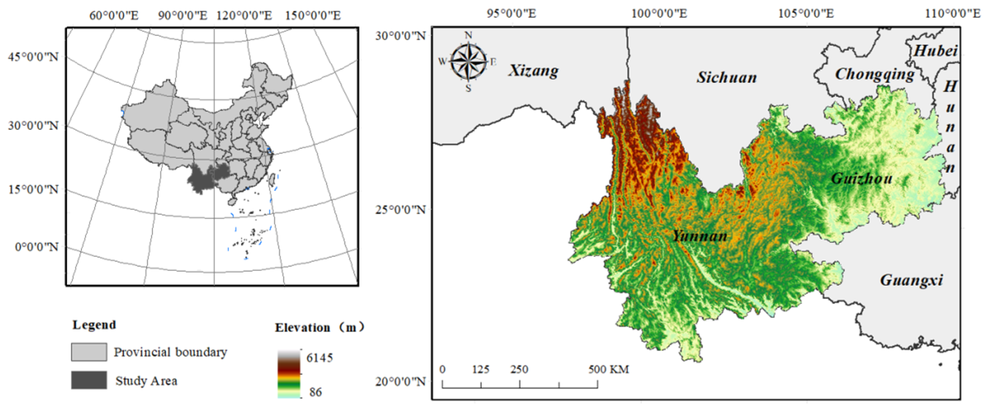
This study focuses on the entirety of Yunnan and Guizhou provinces as the study area (hereinafter referred to as the “Yunnan–Guizhou Plateau”, YGP). Situated in Southwest China, the region covers an administrative area of approximately $\mathrm{570,000} {\mathrm{km}}^2$ [28] and constitutes the main body of the Yunnan–Guizhou Plateau (Figure 1). The YGP lies on the second step of China’s topographical staircase and represents one of the world’s most extensive continuous karst landscapes [29]. The region is characterized by extreme topographic complexity and ecological fragility. The terrain presents a rugged mosaic of precipitous mountains, deep gorges, and fragmented plateaus, with an average elevation of approximately $2000 \mathrm{m}$. This complex topography creates significant vertical zonation and spatial heterogeneity, acting as a dominant physical constraint on land cover patterns [30]. Crucially, the spatial distribution of cropland resources is severely constrained by this high-relief terrain. Croplands are predominantly concentrated in intermontane basins (locally termed “Bazi”) and river valleys, exhibiting a spatial pattern of “macro-dispersion with micro-aggregation”. Outside these flat basins, widely distributed sloping croplands are highly fragmented and irregular, forming intricate landscape mosaics with surrounding forests, shrubs, and grasslands. This unique geomorphology exacerbates the “mixed pixel” phenomenon in 10–30 m resolution satellite imagery, rendering the YGP an ideal testbed for evaluating the robustness of global land cover products in heterogeneous environments [17].

2.2. Data Sources

2.2.1. Land Cover Data Products and Preprocessing

To facilitate a robust assessment of the spatial consistency and regional applicability of multi-source cropland products amidst the complex mountainous terrain of the YGP, this study selected seven high-profile global and regional land cover datasets that are widely recognized within the international scientific community. The selected products are primarily centered on the 2020 baseline to ensure temporal consistency. For datasets where a 2020 version was unavailable (specifically FROM-GLC10), the closest available epoch (2017) was utilized. To justify the temporal comparability given this three-year gap, we conducted a statistical validation using the annual China Land Cover Dataset (CLCD) [9]. The inter-annual comparison reveals high landscape stability in the study area between 2017 and 2020, with 93.44% of cropland pixels remaining spatially consistent and a net total area fluctuation of only 0.12%. Consequently, the potential uncertainty introduced by this temporal mismatch is considered limited relative to the inherent classification errors of global products in complex terrain. These datasets feature two widely adopted spatial resolutions—$10 \mathrm{m}$ and $30 \mathrm{m}$ (

Table 1. Overview of the seven global/regional land cover products used in this study.

Dataset	Res.	Year	Data Source	Classes	Provider	Methodology
GlobeLand30 [7]	30 m	2020	Landsat, HJ-1, GF-1	10	NCSGI	POK-based
CLCD [9]	30 m	2020	Landsat, MODIS	9	WHU	Random Forest
GLC_FCS30 [31]	30 m	2020	Landsat	29	AIR (CAS)	Random Forest
CACD [32]	30 m	2020	Landsat	2	THU	Random Forest
ESA WorldCover [8]	10 m	2020	Sentinel-1 & 2	11	ESA	CatBoost
Esri Land Cover [33]	10 m	2020	Sentinel-2	9	Esri	CNN-UNet
FROM-GLC10 [34]	10 m	2017	Sentinel-2	10	THU	Random Forest

Note: Res. = resolution; POK-based = pixel-object-knowledge-based; NCSGI = National Catalogue Service for Geographic Information; WHU = Wuhan University; AIR (CAS) = Aerospace Information Research Institute, Chinese Academy of Sciences; THU = Tsinghua University; CNN-UNet = convolutional neural network with UNet architecture.

)—corresponding to the Sentinel-2 and Landsat satellite missions, respectively.

The selected datasets originate from diverse scientific consortia (e.g., ESA, Esri, CAS) and were produced using varying satellite sensors (e.g., Sentinel-2, Landsat 8) and classification algorithms (e.g., Random Forest, Deep Learning), and thus exhibit significant multi-source heterogeneity. Although all products include a “cropland” category, discrepancies exist in their delimitation standards—specifically regarding the inclusion of orchards or fallow land—due to variations in classification systems and semantic definitions. To ensure spatial consistency and statistical comparability, a standardized preprocessing framework was implemented: Semantic Reclassification. Based on the technical specifications of each product, we harmonized the cropland definitions (

Table 2. Definitions of cultivated land in the different land cover datasets used in this study.

Dataset	Class Name	Code	Semantic Description
GlobeLand30	Cultivated land	10	Lands used for cultivating crops (including paddy fields, dry farmland, vegetable land, etc.).
CLCD	Cropland	1	Cultivated lands for crops (including mature, new, and fallow cropland; intercropping land with crops as dominant species).
GLC_FCS30	Rain-fed cropland; irrigated cropland	10–12, 20	Cropland dependent on natural precipitation (Codes 10–12); cropland with stable irrigation systems for artificial water supply (Code 20).
CACD	Cropland	1	Land of ≥0.25 ha for annual crop cultivation (excludes perennial crops, greenhouses, and small plots).
ESA WorldCover	Cropland	40	Land used for annual crop cultivation (including fallow land).
Esri Land Cover	Crops	5	Human-planted crops (cereals, soy, etc.) at non-tree height.
FROM-GLC10	Cropland	10	Lands used for agriculture, including arable land, tillage, and paddy fields.

Note: Codes and descriptions were derived from the official user guides of the respective datasets.

).

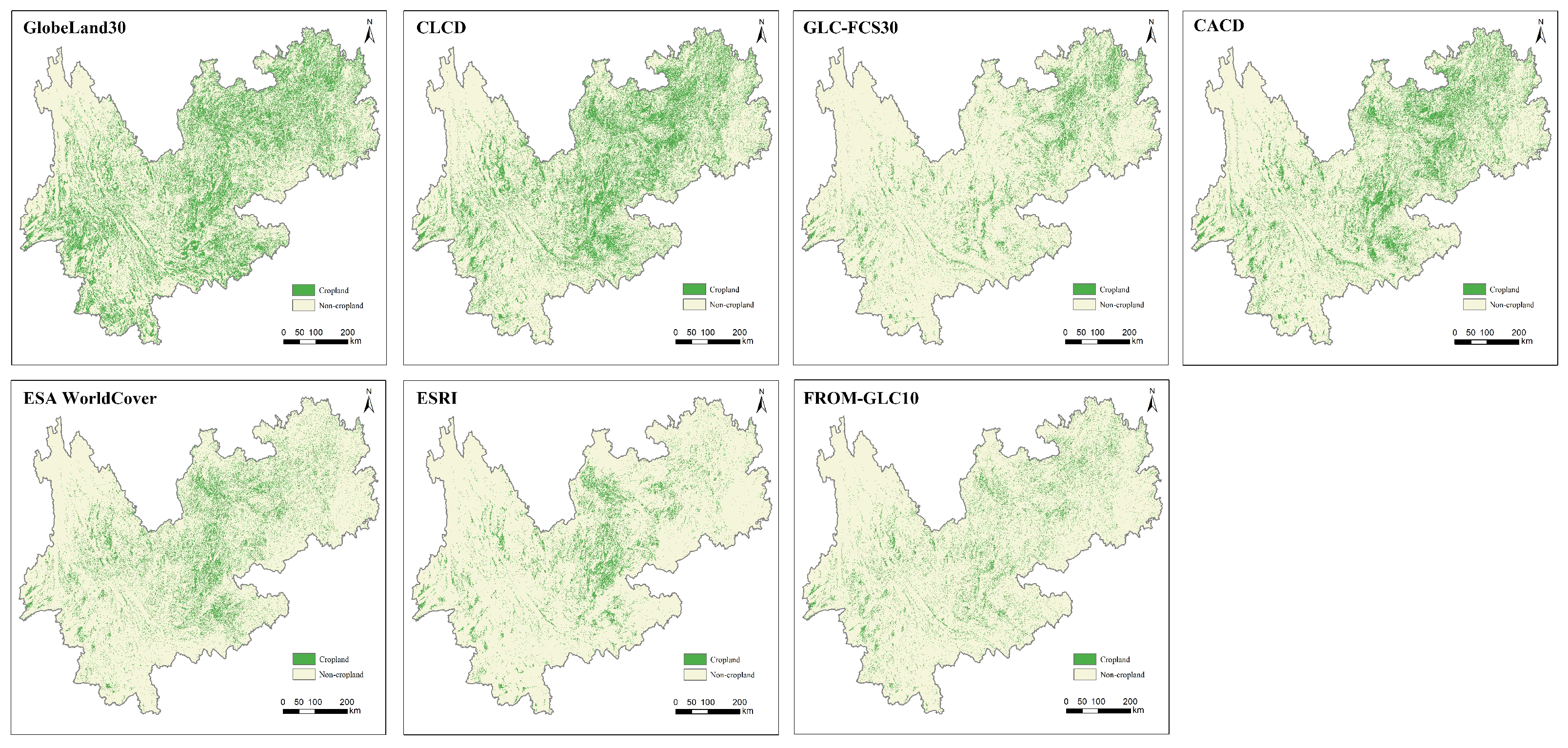
All datasets were reclassified into a binary format: cropland (assigned as 1) and non-cropland (assigned as 0) (Figure 2). Spatial Resampling: To align with the finest resolution among the datasets, all $30 \mathrm{m}$ products were resampled to $10 \mathrm{m}$ using the Nearest Neighbor method to minimize spatial detail and categorical fidelity loss. Reprojection: All datasets were reprojected to the Asia North Albers Equal Area Conic projection (ESRI: 102025). This projection was selected to strictly preserve area properties, thereby eliminating high-latitude geometric distortion and ensuring area-based statistical rigor.

2.2.2. Validation Data

1.

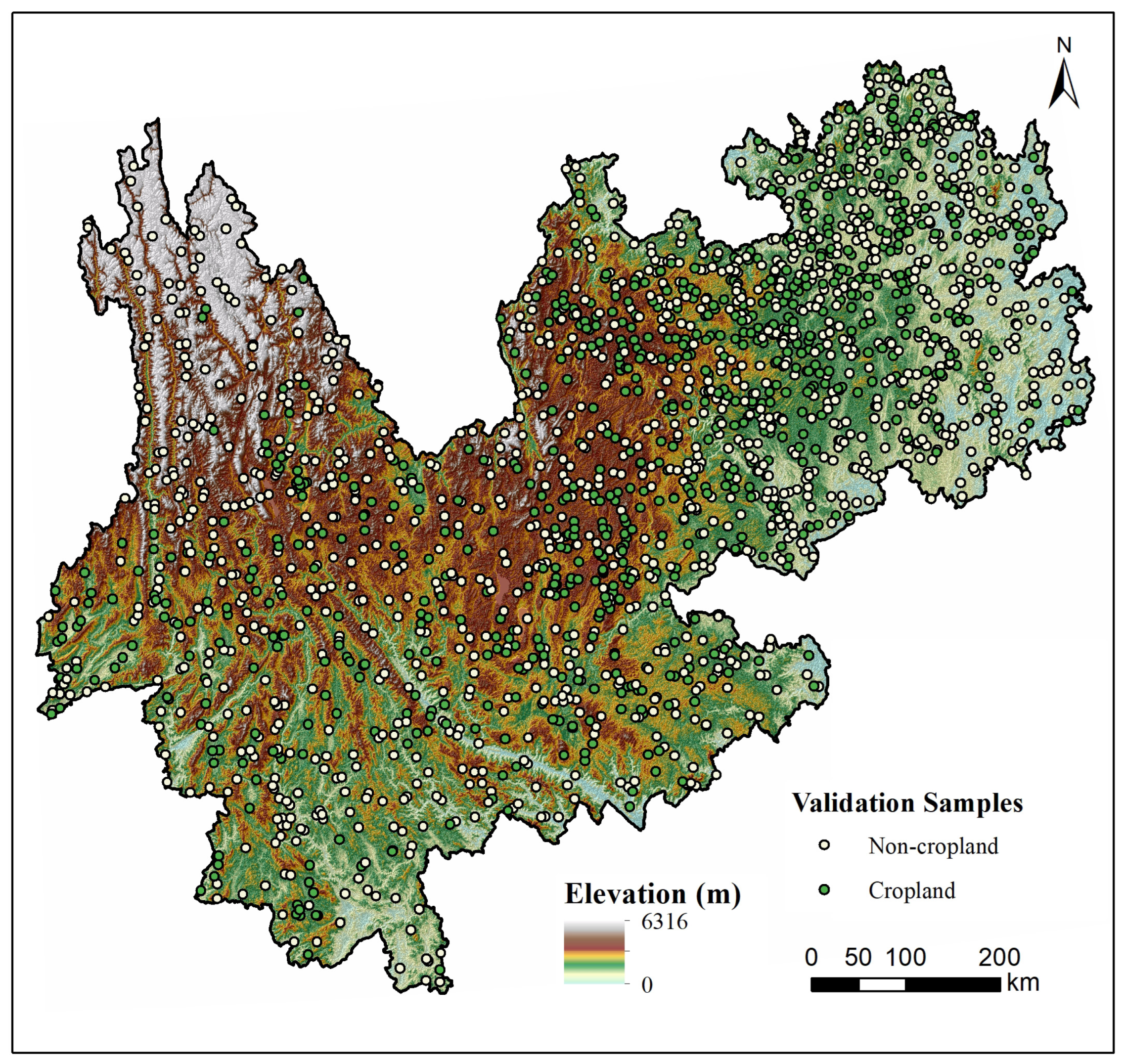
Validation Samples: To rigorously evaluate the classification accuracy of the multi-source products, an independent validation dataset comprising 2000 samples was constructed (Figure 3). These samples were generated using a random sampling strategy and underwent point-by-point visual interpretation based on high-resolution Google Earth imagery. The final validated dataset consists of 785 cropland samples and 1215 non-cropland samples. Spatially speaking, the distribution of these samples covers the diverse topographic environments within the study area, ensuring representative coverage for accuracy assessment.

2.

Land Survey Statistical Data: The statistical data from the Third National Land Survey of China (hereinafter referred to as the “Third Land Survey”), finalized in 2020, was employed as the authoritative reference for cropland area statistics [28]. Covering 217 county-level administrative units within the study area, this dataset not only establishes the total cropland extent of $\mathrm{88,289.78} {\mathrm{km}}^2$ across the Yunnan–Guizhou Plateau, but also serves as a source of high-precision ground truth area values for each county. Serving as a unified benchmark at the administrative statistical scale, these data were utilized to calculate the Area Estimation Bias of each land cover product at the county level, thereby systematically revealing the consistency and reliability of the quantitative characterization of cropland by different products.

Figure 3. Spatial distribution of validation samples in 2020.

Figure 3. Spatial distribution of validation samples in 2020.

2.2.3. Potential Driving Factors

To quantitatively disentangle the spatial heterogeneity and underlying driving mechanisms of discrepancies in cropland mapping across the Yunnan–Guizhou Plateau, this study constructed a multi-dimensional explanatory framework rooted in the “human–environment” system. Informed by prior theoretical and empirical studies of the determinants of land cover classification uncertainty [17,30,35,36], we selected 14 potential covariates spanning four distinct domains: topographic complexity, climatic conditions, landscape fragmentation, and anthropogenic intensity (

Table 3. The system of potential driving factors for cropland mapping inconsistency.

Category	Variable	Abbr.	Description and Ecological Meaning	Res.	Source
Topography	Elevation	Elev.	Mean elevation; restricts cropland distribution.	30 m	NASADEM [37]
	Terrain Relief	Elev_SD	Standard deviation of elevation; reflects vertical roughness.	30 m	NASADEM
	Slope	Slope	Mean slope; affects farming difficulty and runoff.	30 m	NASADEM
	Slope Variability	Slope_SD	Standard deviation of slope; indicates terrain complexity.	30 m	NASADEM
Environment	Cloud Frequency	Cloud	Annual mean frequency of cloud observations calculated from the QA band.	1 km	MODIS
	Rocky Desertification	NDRI	Normalized Difference Rock Index; masked for water.	30 m	Landsat 8
	Phenological Heterogeneity	Pheno. Diff.	Intra-grid range ($Max-Min$) of maize phenology.	1 km	Luo et al. [38]
Landscape	Patch Density	PD	Number of cropland patches per 100 ha; fragmentation intensity.	GRID	Calculated from ESA
	Mean Patch Size	MPS	Average area of cropland patches; distinct from fragmentation.	GRID	Calculated from ESA
	Aggregation Index	AI	Frequency of side-by-side adjacencies; spatial connectivity.	GRID	Calculated from ESA
	Edge Density	ED	Length of edge per unit area; shape complexity.	GRID	Calculated from ESA
	Largest Patch Index	LPI	Percentage of total landscape area comprising the largest patch.	GRID	Calculated from ESA
Anthropogenic	Human Footprint	HFP	Integrated index of human pressure (built-up, lights, etc.).	1 km	Mu et al. [39]
	Cropland Abandonment	Aband. Land	Total area of abandoned cropland per grid.	30 m	Liu et al. [40]

Note: Res. = resolution. GRID = analytical grid cell (10 km × 10 km).

). To ensure spatial compatibility, all covariate layers were harmonized and aggregated to align with the corresponding analytical units (i.e., county-level administrative districts and regular grid cells) employed in the subsequent analysis.

The calculation and processing details for the specific driving factors are as follows:

1.

Cloud Frequency: This was derived from the MODIS Terra Daily Surface Reflectance product (MOD09GA, V6.1) [41] via Google Earth Engine (GEE). We utilized the state_1 km QA band to extract cloud state bits (0–1). The annual mean cloud frequency was generated at 1 km resolution by calculating the ratio of observations flagged as “cloudy” or “mixed” to the total daily observations in 2020. This metric serves as a direct proxy for atmospheric interference intensity.

2.

Rocky Desertification Index: This was computed using Landsat 8 OLI data on GEE. After masking clouds and shadows via the QA_PIXEL band, a median composite was generated for 2020. To prevent water misclassification, pixels with $MNDWI>0$ were masked out. The Normalized Difference Rock Index (NDRI) [42] was calculated as follows to highlight exposed bedrock in karst landscapes:

$$\mathrm{NDRI}={\displaystyle \frac{{\rho }_{\mathrm{SWIR}1}-{\rho }_{\mathrm{NIR}}}{{\rho }_{\mathrm{SWIR}1}+{\rho }_{\mathrm{NIR}}}}$$

(1)

where ${\rho }_{\mathrm{SWIR}1}$ and ${\rho }_{\mathrm{NIR}}$ represent surface reflectance in the shortwave infrared and near-infrared bands, respectively.

3.

Phenological Heterogeneity: Utilizing the ChinaCropPhen1km dataset [38], we extracted key phenological dates for maize. The phenological range ($Max-Min$) within each analytical grid was calculated to quantify growth asynchrony. A larger range indicates diverse growth stages within a grid, causing high spectral heterogeneity (“same object, different spectra”) that challenges consistent mapping.

4.

Landscape Metrics: To minimize the propagation of classification errors, landscape indices were computed based on the ESA WorldCover (the product with the highest accuracy, see Section 3.1) using the landscapemetrics R package [43]. Five class-level metrics—patch density (PD), Mean Patch Size (MPS), edge density (ED), Largest Patch Index (LPI), and Aggregation Index (AI)—were derived to quantify the cropland landscape’s fragmentation and spatial connectivity [44].

5.

Cropland Abandonment: Data was obtained from the Cropland Abandonment in China Dataset [40]. We calculated the total pixel count of abandoned cropland within each analytical grid. A higher frequency of abandonment implies a higher probability of spectral ambiguity, as these transitional lands often exhibit mixed signals of active crops and recovering vegetation.

2.3. Research Methods

To ensure methodological rigor and avoid terminological ambiguity, we explicitly define the three core performance metrics used throughout this study. Accuracy refers to the correctness of a land cover product, quantified by its agreement with independent reference data (e.g., the Third National Land Survey), measuring “how close the map is to the ground truth.” Consistency denotes the degree of agreement among multiple satellite-derived products at a specific location, independent of validation samples, reflecting the consensus among different sensors and algorithms. In this study, Uncertainty is operationally defined as the spatial divergence among products; we use low consistency as a proxy for mapping uncertainty to identify regions where current algorithms fail to converge. Based on these operational definitions, the evaluation framework is organized into the following three parts.

2.3.1. Accuracy and Area Comparison

1.

Area Estimation and Correlation Analysis

We first computed the total area and proportion of cropland for all seven products to reveal discrepancies in the extent of mapped cropland. Furthermore, using the Third National Land Survey data as the ground truth, we performed a correlation analysis across 217 county-level units. The Pearson correlation coefficient (r) and Root Mean Square Error (RMSE) were calculated to assess the consistency between the product estimates and the survey data. This quantitative evaluation determines the reliability of each dataset in characterizing cropland area at the administrative scale, identifying systematic overestimation or underestimation caused by differing classification definitions (e.g., GlobeLand30’s broad definition) or temporal inconsistencies. It is important to note that this aggregate metric primarily reflects quantity agreement for regional inventory. We explicitly acknowledge the potential cancellation effect in statistical data, where pixel-level commission and omission errors may offset each other. Therefore, this analysis is complemented by pixel-level confusion matrix assessment to evaluate true spatial accuracy.

2.

Confusion Matrix-based Accuracy Assessment

To evaluate the pixel-level classification performance, we employed a binary confusion matrix using the validation samples described in Section 2.2.2. Defining “cropland” and “non-cropland” as the positive and negative classes, respectively, we derived four metrics: True Positive (TP), False Positive (FP), True Negative (TN), and False Negative (FN). Based on these, we calculated Overall Accuracy (OA), Producer’s Accuracy (PA), User’s Accuracy (UA), F1 Score, and the Matthews Correlation Coefficient (MCC) to comprehensively measure classification performance:

$$OA={\displaystyle \frac{TP+TN}{TP+TN+FP+FN}}$$

(2)

$$PA={\displaystyle \frac{TP}{TP+FN}}$$

(3)

$$UA={\displaystyle \frac{TP}{TP+FP}}$$

(4)

$$F1={\displaystyle \frac{2\times PA\times UA}{PA+UA}}$$

(5)

$$MCC={\displaystyle \frac{TP\times TN-FP\times FN}{\sqrt{(TP+FP)(TP+FN)(TN+FP)(TN+FN)}}}$$

(6)

2.3.2. Spatial Consistency Assessment Metrics

1.

Pairwise Spatial Similarity (Jaccard)

To quantify the spatial agreement in cropland distribution between different products, we employed the Jaccard similarity coefficient, also referred to as the Intersection over Union (IoU) [45]. This metric calculates the ratio of the intersection area to the union area of the target class, ranging from 0 (no overlap) to 1 (perfect spatial match):

$$J(A,B)={\displaystyle \frac{|A\cap B|}{|A\cup B|}}$$

(7)

where A and B denote the sets of identified cropland pixels in the two comparative datasets. In this study, the Jaccard coefficient serves as a sensitive indicator for evaluating the consistency of boundary delineation within the fragmented mountainous terrain.

2.

Pixel-level Consistency Aggregation

To assess the spatial agreement among all seven products simultaneously, we conducted a pixel-level overlay analysis. We stacked the binary cropland maps of all products and summed the values for each pixel to generate a Consistency Level ($CL$) map, ranging from 0 to 7.

• $CL=0$: No product identifies the pixel as cropland (excluded from analysis).
• $CL=1$ to 6: Low to moderate consistency, indicating disagreement among products.
• $CL=7$: High consistency, where all products agree on the cropland label.

Based on the consistency level map, we calculated the area proportion of each consistency level to reveal the uncertainty of class boundaries in complex geomorphic contexts. The consistency ratio for level i is defined as follows:

$$P_i={\displaystyle \frac{{\mathrm{Area}}_i}{{\sum }_{i=1}^7{\mathrm{Area}}_i}}\times 100\%$$

(8)

where ${\mathrm{Area}}_i$ is the total area of pixels with consistency level i.

2.3.3. Analysis of Driving Mechanisms

To disentangle the explanatory power and spatial non-stationarity of the factors (defined in Section 2.2.3) driving cropland mapping inconsistency, we employed two complementary statistical models: the Optimal Parameter-based Geographical Detector (OPGD) [46] and Multiscale Geographically Weighted Regression (MGWR) [47]. To comprehensively elucidate the driving mechanisms across different granularities, all analyses were conducted at two distinct spatial scales:

• County-level Administrative Scale: As the fundamental unit of agricultural policy implementation and statistical governance in China, this scale allows for assessing consistency from a macro-management perspective.
• 10 km Grid Scale: Following the geostatistical framework established by Zou et al. [48], this scale was explicitly selected to reduce the estimate deviation triggered by spatial data homogeneity. It acts as a spatial filter to optimize the trade-off between capturing regional structural characteristics and mitigating the local noise inherent to high-resolution data, thereby revealing robust fine-grained spatial heterogeneity.

1.

Optimal Parameter Geographical Detector

The Factor Detector within OPGD was applied at both the county and grid scales to reveal scale-dependent driving mechanisms. The q-value measures the degree to which a factor X explains the spatial stratification of the consistency index Y:

$$q=1-{\displaystyle \frac{{\sum }_{h=1}^L{N}_h{\sigma }_h^2}{N{\sigma }^2}}$$

(9)

where $h=1,\dots ,L$ are the strata of factor X; $N_h$ and ${\sigma }_h^2$ denote the number of units and the variance of Y within stratum h, respectively; and N and ${\sigma }^2$ are the total number of units and the variance of Y over the entire region, respectively. A higher q value indicates a stronger driving force.

2.

Multiscale Geographically Weighted Regression

While OPGD reveals the global explanatory power of drivers, the relationships between covariates and mapping consistency may exhibit spatial non-stationarity. To capture these spatially varying effects, we utilized MGWR. Unlike classical Geographically Weighted Regression (GWR), which assumes a constant bandwidth for all variables, MGWR allows each covariate to possess a unique optimal bandwidth. This flexibility enables the model to correctly reflect the distinct spatial scales at which different processes operate:

$$y_i={\beta }_0(u_i,v_i)+\sum _{k=1}^m{\beta }_{bwk}(u_i,v_i)x_{ik}+{ϵ}_i$$

(10)

where $(u_i,v_i)$ are the coordinates of location i and ${\beta }_{bwk}$ represents the local coefficient for the k-th variable with a specific bandwidth $bwk$. This approach allows for the visualization of local parameter estimates, highlighting how specific factors differentially impact mapping consistency across the heterogeneous plateau landscape.

3. Results

3.1. Accuracy Assessment and Area Comparison of Cropland Products

3.1.1. Comparison of Cropland Area Estimates

Using the Third National Land Survey ($\mathrm{87,929.79} {\mathrm{km}}^2$, accounting for $15.42\%$ of the total area) as the authoritative benchmark, the seven products exhibited a sharp polarization in area estimation (Table 4). This divergence underscores how high spatial resolution alone does not guarantee statistical accuracy in complex terrains.

• Significant Overestimation: GlobeLand30, CLCD, and CACD considerably overestimated cropland extent. GlobeLand30 showed the largest deviation, exceeding the benchmark by nearly $87.5\%$, primarily due to the spectral confusion between sloping cropland and other vegetation types (e.g., shrubs and forests) in mountainous areas.
• Significant Underestimation: Conversely, GLC-FCS30, FROM-GLC10, and Esri Land Cover were conservative. The latter produced the lowest estimate ($\mathrm{51,136.79} {\mathrm{km}}^2$), capturing only about $58\%$ of the benchmark area ($9.14\%$ vs. $15.42\%$), indicating severe omission errors in identifying fragmented croplands.
• Highest Consistency: ESA WorldCover demonstrated the closest agreement with the survey data. Although it underestimated the total area by roughly $13.8\%$ ($\mathrm{75,772.08} {\mathrm{km}}^2$), it offered the most robust and accurate representation of total cropland quantity among the evaluated datasets.

Table 4. Statistics of cultivated land area in the Yunnan–Guizhou region derived from seven land cover products.

Product/Dataset	Area (${\mathbf{km}}^2$)	Proportion (%)
Third National Land Survey	87,929.79	15.42
GlobeLand30	164,880.04	29.48
CLCD	142,279.14	25.44
CACD	109,329.88	19.55
ESA WorldCover	75,772.08	13.55
GLC_FCS30	64,181.33	11.48
FROM-GLC10	52,880.96	9.46
Esri Land Cover	51,136.79	9.14

Table 4. Statistics of cultivated land area in the Yunnan–Guizhou region derived from seven land cover products.

Product/Dataset	Area (${\mathbf{km}}^2$)	Proportion (%)
Third National Land Survey	87,929.79	15.42
GlobeLand30	164,880.04	29.48
CLCD	142,279.14	25.44
CACD	109,329.88	19.55
ESA WorldCover	75,772.08	13.55
GLC_FCS30	64,181.33	11.48
FROM-GLC10	52,880.96	9.46
Esri Land Cover	51,136.79	9.14

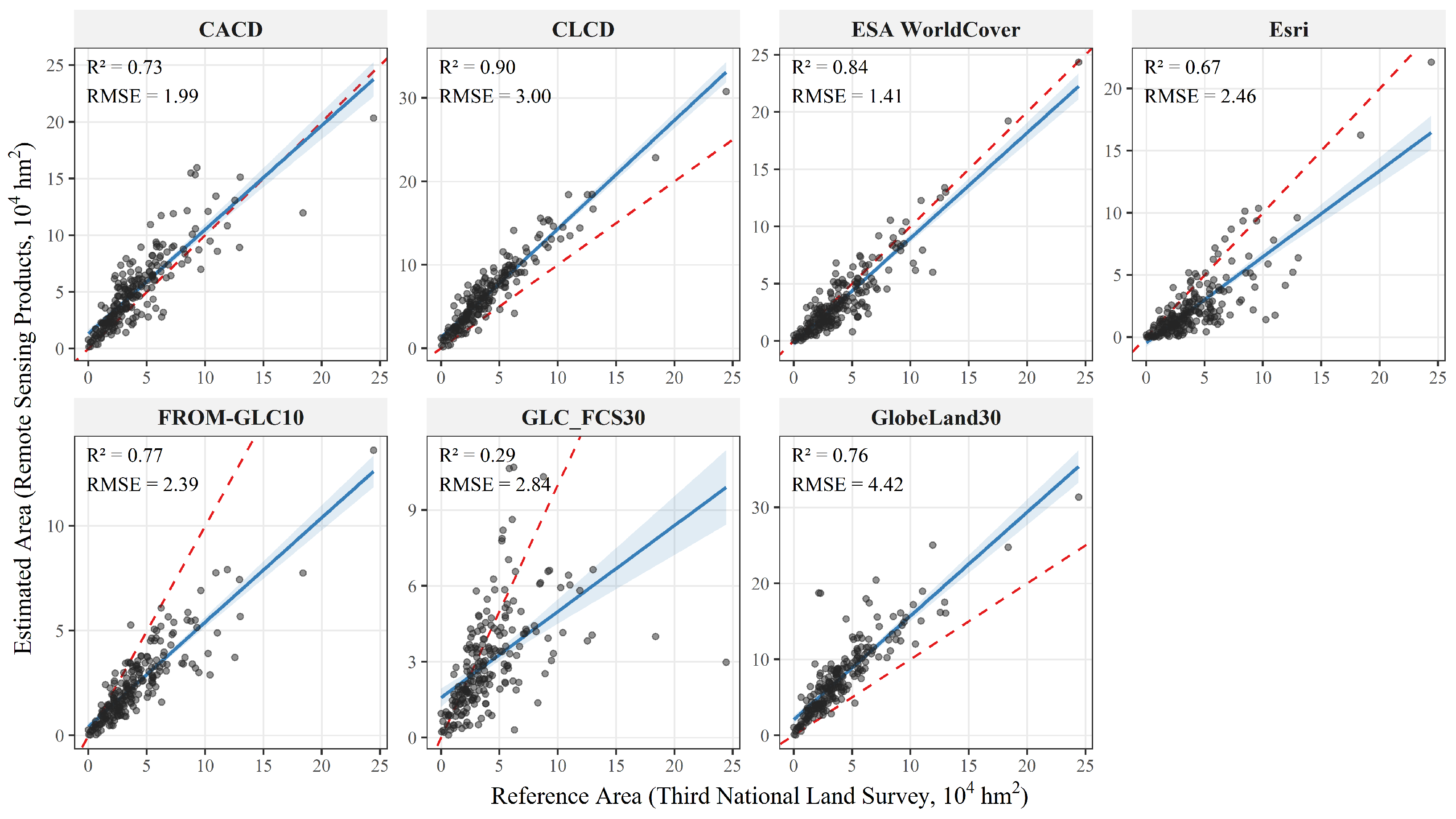
To further evaluate the statistical reliability of the land cover products at the administrative scale, we performed a linear regression analysis across 217 county-level units, employing the Third National Land Survey data as the benchmark. The coefficient of determination ($R^2$) and Root Mean Square Error (RMSE) were calculated to quantify the agreement between the satellite-derived cropland areas and the official reference statistics (Figure 4).

The regression results revealed significant disparities in product performance. CLCD achieved the highest coefficient of determination ($R^2=0.90$), suggesting the strongest capability in capturing spatial heterogeneity and relative distribution trends across counties, followed closely by ESA WorldCover ($R^2=0.84$). In contrast, GLC_FCS30 exhibited the poorest stability with a significantly low correlation ($R^2=0.29$). However, high correlation did not necessarily equate to accurate area estimation, as systematic deviations from the 1:1 identity line were evident. GlobeLand30, CLCD, and CACD generally overestimated cropland area; notably, while CLCD possessed the best linear fit, its steep regression slope resulted in a high RMSE of $3.00\times {10}^4 {\mathrm{hm}}^2$, whereas GlobeLand30 exhibited the largest error magnitude (RMSE = $4.42\times {10}^4 {\mathrm{hm}}^2$). Conversely, Esri, FROM-GLC10, and GLC_FCS30 showed a consistent underestimation trend, with Esri yielding an RMSE of $2.46\times {10}^4 {\mathrm{hm}}^2$. Ultimately, ESA WorldCover achieved the optimal balance between correlation and accuracy, with scatter points tightly clustered around the 1:1 line and the lowest RMSE ($1.41\times {10}^4 {\mathrm{hm}}^2$), identifying it as the most robust product for quantitative cropland estimation at the county scale.

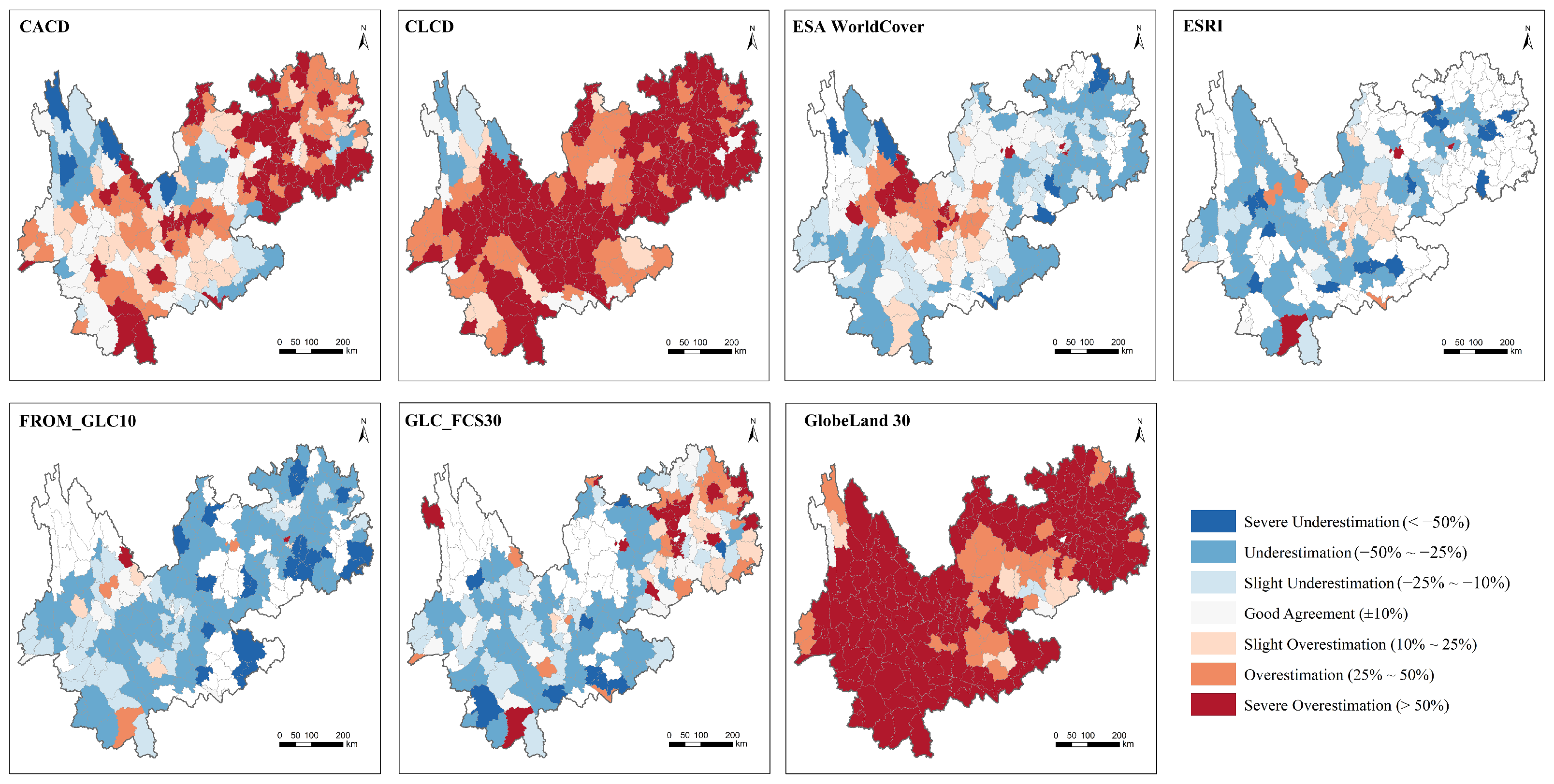
To visually characterize the spatial heterogeneity of estimation bias, we calculated the Relative Error ($RE$) for each county and classified the results into seven levels ranging from “Severe Underestimation” (<$-50\%$) to “Severe Overestimation” (>$50\%$), with deviations within $\pm 10\%$ defined as “Good Agreement” (Figure 5).

The spatial patterns reveal distinct clustering of errors consistent with the regression analysis. GlobeLand30 and CLCD exhibit the most extensive systematic bias, with the majority of the region classified as severe overestimation (>$50\%$), indicating a pervasive inflation of cropland area independent of spatial location. A similar trend was observed in CACD, although its overestimation was predominantly concentrated in the Guizhou region. Conversely, Esri, FROM-GLC10, and GLC_FCS30 are characterized by widespread underestimation, particularly in the rugged western and northern high-altitude regions, suggesting a failure to detect fragmented croplands. ESA WorldCover demonstrates the most robust performance, achieving good agreement in central regions, despite exhibiting minor spatial heterogeneity with overestimation in central and western Yunnan and underestimation in the eastern part of the study area (Guizhou).

3.1.2. Accuracy Assessment Based on Validation Samples

As presented in

Table 5. Accuracy assessment of the seven land cover products based on the validation samples. The 95% confidence intervals (CI) for Overall Accuracy are calculated based on the binomial distribution ($N=2000$).

Product	OA (95% CI)	UA	PA	F1	MCC	Kappa
ESA WorldCover	0.81 (±0.017)	0.85	0.63	0.72	0.60	0.72
FROM-GLC10	0.75 (±0.019)	0.83	0.47	0.60	0.48	0.44
GlobeLand30	0.74 (±0.019)	0.63	0.74	0.70	0.48	0.47
CLCD	0.74 (±0.019)	0.62	0.88	0.73	0.53	0.50
Esri Land Cover	0.74 (±0.019)	0.85	0.43	0.57	0.47	0.42
CACD	0.72 (±0.020)	0.59	0.89	0.71	0.49	0.71
GLC_FCS30	0.72 (±0.020)	0.70	0.53	0.60	0.40	0.40

Note: OA: Overall Accuracy; CI: Confidence Interval; UA: User’s Accuracy; PA: Producer’s Accuracy; MCC: Matthews Correlation Coefficient.

, ESA WorldCover demonstrated superior overall classification performance among the evaluated datasets, achieving the highest Overall Accuracy (0.81) and Matthews Correlation Coefficient (0.60). This indicates its strong capability in differentiating cropland from complex background features. In terms of class-specific accuracy, the products exhibited divergent performance patterns that align with the area estimation biases observed earlier. CLCD and CACD were characterized by exceptionally high Producer’s Accuracies (>$0.88$), implying a strong ability to detect cropland pixels; however, their relatively low User’s Accuracies (0.62 and 0.59, respectively) reveal significant commission errors, confirming that the substantial area overestimation was driven by the misclassification of non-cropland categories. Conversely, Esri and FROM-GLC10 prioritized precision over complete detection, attaining high User’s Accuracies (>$0.83$) but suffering from severe omission errors, as evidenced by their low Producer’s Accuracies (0.43 and 0.47). This indicates that while the cropland pixels identified by these products are highly reliable, they failed to capture more than half of the actual cropland in the region. Ultimately, although ESA WorldCover also exhibited moderate omission errors (PA = 0.63), it maintained the most effective balance between commission and omission, yielding a high F1-score (0.72) and validating its robustness as the most reliable product for regional cropland mapping.

3.2. Spatial Consistency Analysis

3.2.1. Pairwise Spatial Similarity

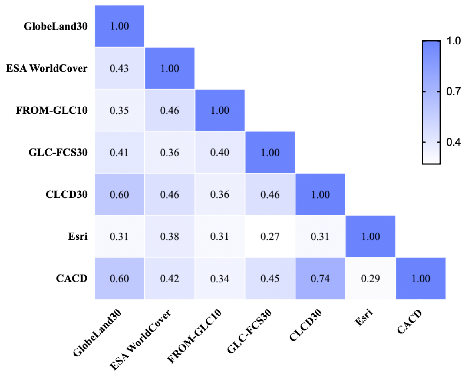
The Jaccard similarity coefficients (Figure 6) quantify the pixel-level spatial agreement of cropland among the seven products, ranging from 0.27 to 0.74. This substantial variation reveals distinct clustering patterns driven by data provenance and classification strategies:

• High-Consistency Cluster (Landsat-based): A robust high-consistency group was observed among CLCD, CACD, and GlobeLand30. Notably, CLCD and CACD exhibited the highest pairwise similarity ($0.74$), and their respective agreements with GlobeLand30 both reached $0.60$. This strong spatial consensus is likely attributable to their shared lineage, as all three datasets primarily rely on Landsat imagery, leading to similar spectral feature extraction capabilities.
• Moderate Consistency (Sentinel-2-based): ESA WorldCover served as a moderate bridge, displaying intermediate agreement with other datasets ($0.36$–$0.46$). While its 10 m resolution effectively captures fragmented cropland structures, its geometric precision introduces systematic deviations when overlaid with coarser 30 m products, preventing higher Jaccard values.
• Low Consistency and Outliers: Esri Land Cover emerged as a distinct outlier, yielding the lowest similarity indices ($0.27$–$0.38$) across the board. This weak spatial overlap corroborates its severe area underestimation identified in Section 3.1.1. Furthermore, even between products with similar specifications (e.g., GLC_FCS30 and FROM–GLC10), the consistency was limited ($0.40$), suggesting that differences in temporal phases and classification algorithms introduce significant uncertainty in boundary delineation within these fragmented terrains.

Figure 6. Spatial consistency of cultivated land and heatmap of Jaccard similarity coefficient.

Figure 6. Spatial consistency of cultivated land and heatmap of Jaccard similarity coefficient.

3.2.2. Spatial Patterns of Consistency Levels

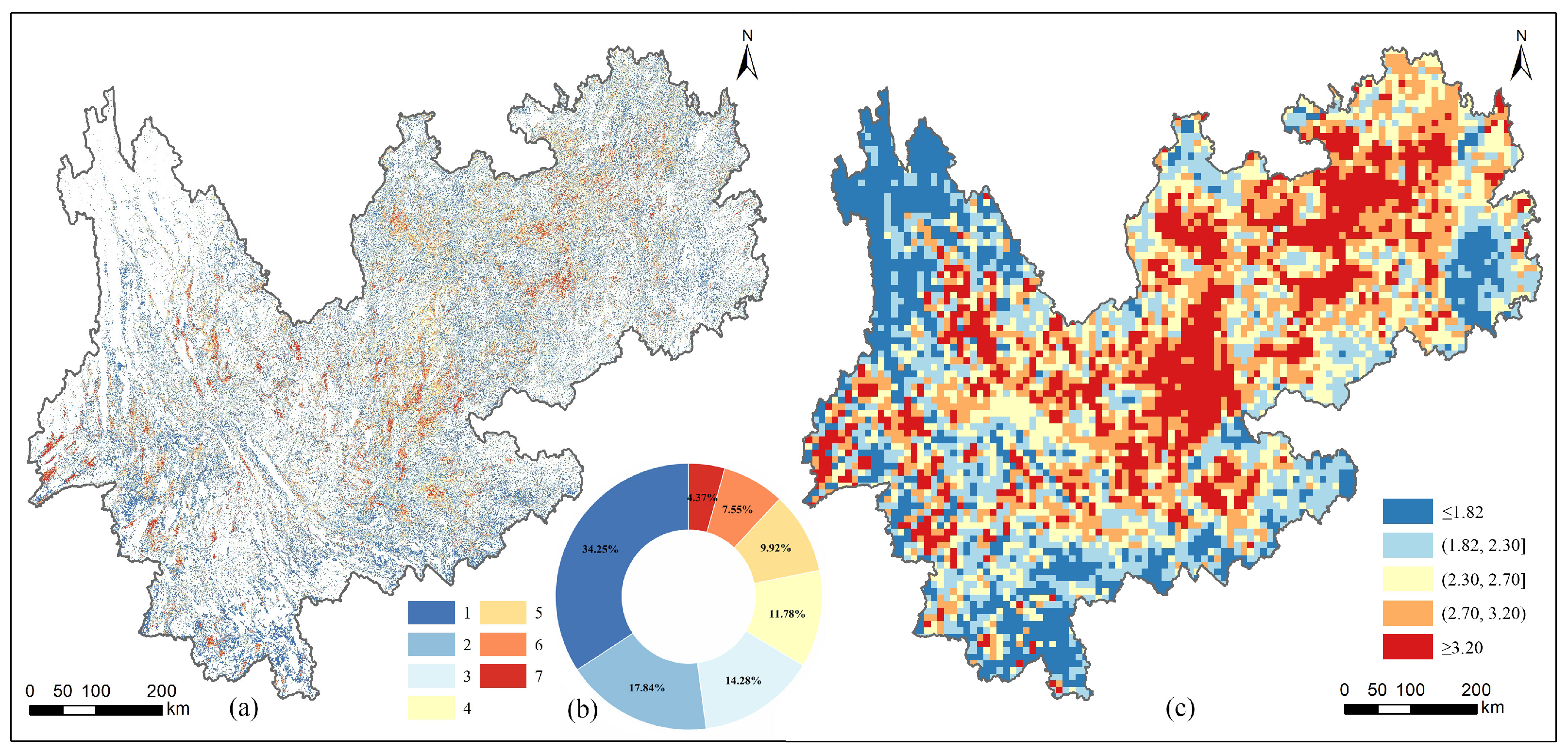
To comprehensively evaluate the reliability of cropland identification, this study integrates pixel-level spatial distribution, quantitative statistical characteristics, and grid-scale aggregation analysis to characterize the consistency patterns across the Yunnan–Guizhou Plateau (Figure 7).

Spatially, the pixel-level distribution map (Figure 7a) reveals that low-consistency pixels (Levels 1–2) are widely distributed across the rugged karst landscapes of Southeast Guizhou and the high-altitude mountainous regions of Western Yunnan. In these areas, severe landscape fragmentation and the prevalence of mixed pixels result in significant divergence in boundary delineation among products. Conversely, high-consistency clusters (Levels 6–7) are primarily confined to flat river valleys and central intermontane basins (bazi). The large, continuous cropland patches in these regions facilitate consistent detection across different sensors. Quantitatively speaking, as illustrated in the statistical breakdown (Figure 7b), the areal proportion exhibits a distinct monotonic decrease as the consistency level increases. The study area is dominated by low-consistency regions; notably, Level 1 alone accounts for 34.25% of the total identified cropland. When combined with Level 2 (17.84%), over half of the potential cropland extent lacks broad consensus among the seven products. In contrast, high-certainty areas are scarce. Representing full consensus, Level 7 covers only 4.37% of the region, highlighting the challenge of achieving multi-product agreement in such complex terrain. At the macro scale, the 10 km grid-scale average consistency map (Figure 7c) further corroborates this spatial heterogeneity. The grid analysis effectively mitigates pixel-level noise, highlighting a distinct “core–periphery” structure. The majority of grid cells along the western and northern fringes exhibit extremely low average scores (<$1.82$), marked by deep blue tones, confirming the widespread uncertainty in these rugged zones. Meanwhile, the central and eastern basins emerge as distinct high-value clusters (average score $> 3.20$), visually demonstrating the “hotspots” of reliable cropland identification.

3.3. Driving Mechanisms of Cropland Mapping Inconsistency

3.3.1. Dominant Drivers Identified by OPGD

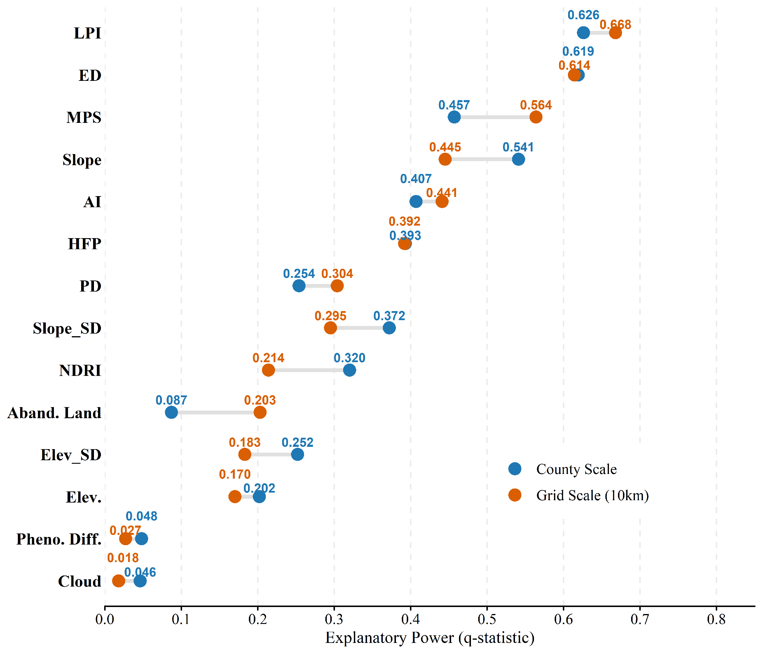
The OPGD was utilized to quantify the explanatory power (q-statistic) of driving factors at both the grid ($10 \mathrm{km}$) and county scales. The results (Figure 8) reveal that landscape configuration and topographic conditions are the dominant drivers of cropland consistency, although their relative importance varies with spatial scale.

The OPGD results identify landscape configuration and topographic conditions as the dominant drivers of cropland consistency across both scales, though their influence exhibits distinct scale dependencies. Landscape metrics consistently demonstrated the highest explanatory power; more specifically, the LPI achieved the highest q-value at the grid scale (0.668), mirrored by strong performance at the county scale (0.626). Along with ED and MPS, these results underscore that spatial structure—particularly patch integrity and fragmentation—serves as the fundamental constraint on classification agreement, where small, disconnected patches and complex boundaries exacerbate mixed pixel effects. Crucially, a cross-scale comparison reveals that the explanatory power of these landscape metrics is amplified at the finer grid scale (e.g., MPS: $0.564>0.457$), suggesting that fragmentation impacts are localized phenomena better captured at high resolutions ($10 \mathrm{km}$). In contrast, topographic influence attenuates at the grid scale; slope exhibited higher explanatory power at the county level ($q=0.541$) compared to the grid level ($q=0.445$), indicating that it acts as a macro-scale regulatory constraint effective over larger administrative units. Additionally, anthropogenic factors represented by HFP maintained moderate influence ($q\approx 0.39$) at both scales, whereas climatic variables remained negligible ($q<0.03$) despite their statistical significance.

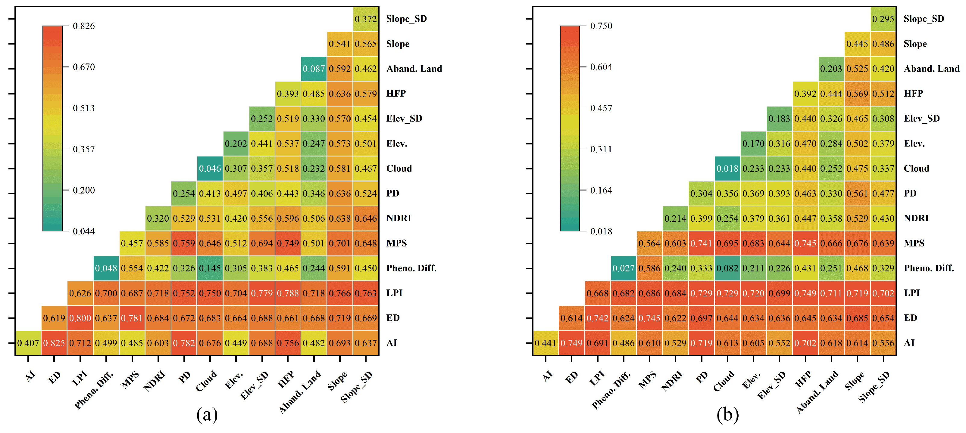
While single-factor analysis identifies dominant drivers, environmental variables often operate synergistically rather than in isolation. To decipher these complex coupling mechanisms, we applied the interaction detector to assess the combined explanatory power of factor pairs. Figure 9 illustrates the interaction matrices for the county scale (a) and grid scale (b). The results demonstrate a universal enhancement effect, where the q-statistic for any pair of factors is invariably greater than that of either single factor acting alone. This confirms that the spatial inconsistency of cropland identification is driven by the mutually reinforcing effects of multiple constraints rather than isolated variables. More specifically, the strongest explanatory power was consistently observed in the interactions between internal landscape metrics. For instance, the interaction between Edge Density (ED) and Aggregation Index (AI) yielded the highest values, suggesting that the coupling of complex boundary shapes and low spatial aggregation creates the most challenging scenario for multi-product consensus. Furthermore, anthropogenic factors such as human footprint showed strong synergy with landscape metrics like LPI, indicating that human-induced disturbance exacerbates landscape fragmentation, thereby degrading classification consistency.

A comparative analysis between scales reveals synergistic drivers’ distinct amplification effect at a coarser resolution, while single landscape metrics exhibited higher sensitivity at the grid scale, their interaction effects were significantly magnified when aggregated to the county level. The interaction q-value between ED and AI surged from 0.749 at the grid scale to 0.825 at the county scale, implying that the macro-structure of cropland—particularly the combination of high edge density and spatial disaggregation—becomes the decisive determinant of consistency for administrative units. Moreover, edge density emerged as a ubiquitous dominant factor in the top interaction pairs at the county scale, unequivocally identifying edge complexity as the critical bottleneck. This suggests that while local fragmentation dictates pixel-level agreement, the cumulative effect of complex boundaries and human disturbance fundamentally limits the ability of different products to achieve consensus at the regional policymaking scale.

3.3.2. Spatial Heterogeneity of Driving Forces (MGWR)

To delineate the spatial non-stationarity of driving mechanisms and identify the specific scales at which different factors operate, we employed the MGWR model. This approach allows us to move beyond global averages and diagnose local variations in the relationship between environmental constraints and cropland consistency.

To verify the presence of spatial non-stationarity in the driving mechanisms, we compared the global Ordinary Least Squares (OLS) baseline with the local MGWR model.

Table 6. Comparison of model performance diagnostics between OLS and MGWR at county and grid scales.

Scale	Model	N	Model Fit		Complexity
			${\mathit{R}}^{\mathbf{2}}$	Adj. ${\mathit{R}}^{\mathbf{2}}$	AICc	Residual ${\mathit{\sigma }}^{\mathbf{2}}$
County	OLS	217	0.814	0.802	5.28	–
	MGWR	217	0.902	0.886	184.38	0.114
Grid	OLS	5995	0.805	0.804	4315.68	–
	MGWR	5995	0.930	0.923	2366.33	0.078

Note: N denotes the number of sample units. The significant increase in adjusted $R^2$ indicates that MGWR captures spatial heterogeneity more effectively than OLS.

presents a diagnostic comparison between the global OLS baseline and the local MGWR model at both county and grid scales, while the OLS model provided a reasonable baseline (Adj. $R^2\approx 0.80$), the MGWR model demonstrated superior explanatory power. More specifically, at the grid scale, the Adj. $R^2$ improved significantly to 0.923, and the AICc value decreased substantially from 4315.68 to 2366.33. This marked improvement confirms that the driving forces of cropland consistency exhibit significant spatial heterogeneity, which global models fail to capture. Consequently, the MGWR results provide a more reliable basis for identifying regional bottlenecks.

A unique advantage of MGWR is its ability to determine optimal bandwidths, revealing each variable’s operating scale. As summarized in

Table 7. Comparison of optimal bandwidths (operating scales) for key driving factors identified by MGWR at county and grid scales.

Category and Variable	County Scale ($\mathit{N}=217$)		Grid Scale ($\mathit{N}=5995$)
	Bandwidth (km)	Scale Type	Bandwidth (km)	Scale Type
Topography
Slope	∼1384		∼72	Local
Slope_SD	∼1384	Global	∼1485	Global
Elev.	∼412	Regional	∼72	Local
Elev_SD	∼1384	Global	∼1485	Global
Environment
Cloud	∼412	Regional	∼364	Regional
NDRI	∼783	Regional	∼78	Local
Landscape
ED	∼1384	Global	∼1485	Global
LPI	∼1384		∼72	Local
MPS	∼412	Regional	∼230	Regional
PD	∼1384	Global	∼72	Local
AI	∼1384	Global	∼72	Local
Anthropogenic
HFP	∼1384	Global	∼102	Local
Aband. Land	∼412	Regional	∼454	Regional

Note: Bandwidth indicates the spatial range of influence. A large bandwidth (approximating the study area size) implies spatial stationarity (Global), while a small bandwidth implies high spatial heterogeneity (Local).

, the results highlight a distinct “Global-to-Local” transition as the analysis resolution becomes finer. Edge density (ED) consistently exhibits a global bandwidth (∼1384–1485 km) across both scales, indicating that boundary fragmentation is a ubiquitous constraint with a relatively stationary impact throughout the plateau. In contrast, factors such as Mean Slope and LPI, which appear as global variables at the county scale, shift to highly localized scales (∼72 km) in the grid-level analysis. This suggests that the influence of topography and patch integrity is masked by averaging at the administrative level but reveals intense local sensitivity when observed at a finer resolution.

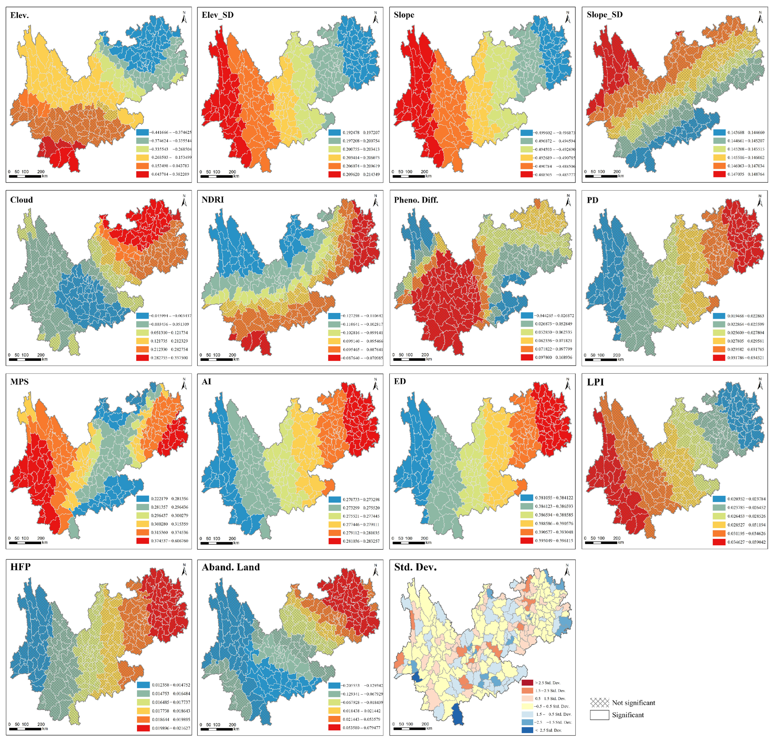
At the county scale, the MGWR results reveal a markedly more homogenized spatial pattern relative to the grid scale (Figure 10). Attributable to the smoothing effect of spatial aggregation, the majority of driving factors manifest high spatial stationarity, characterized by relatively consistent regression coefficients across administrative units.

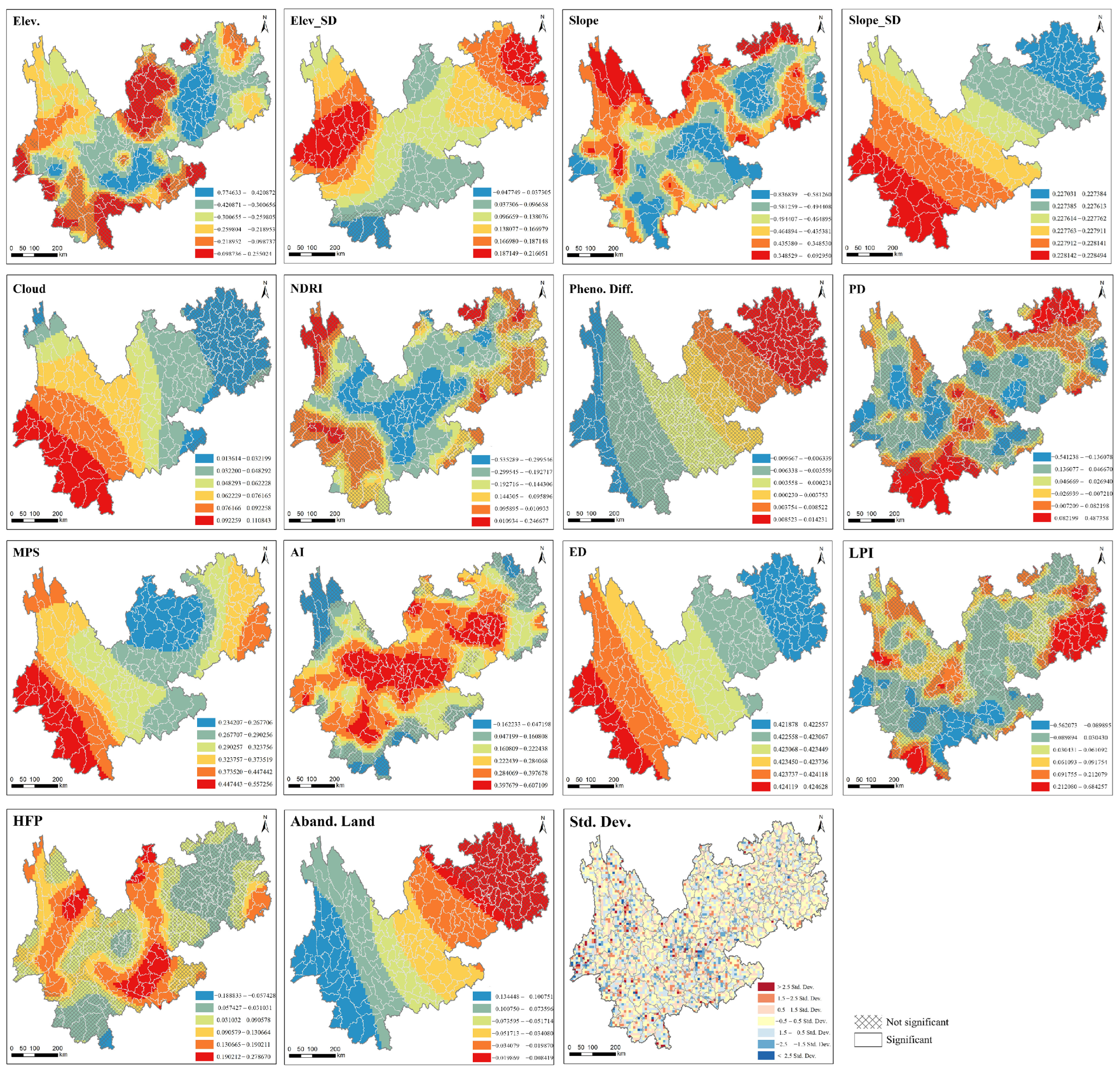
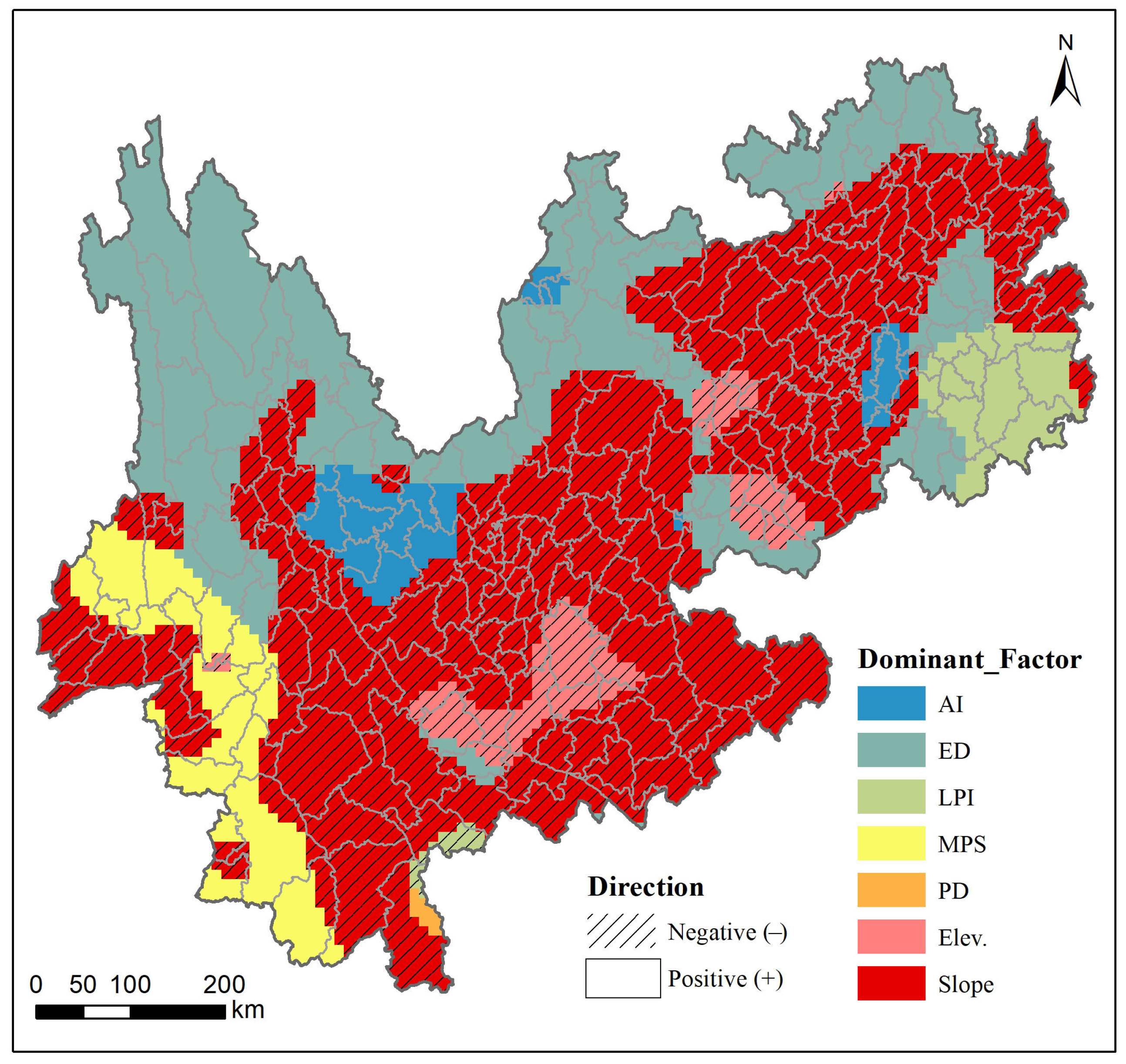
The grid-scale MGWR analysis demonstrates a robust model fit with minimal local bias, corroborated by standardized residuals that are predominantly distributed within the narrow range of −0.5 to 0.5 (Figure 11). Significance testing further elucidates the spatial constraints on explanatory power: masked (cross-hatched) areas ($p>0.05$) indicate that phenological difference (PD) lacks statistical significance across extensive regions, while the significant effects of LPI and PD are confined to highly localized pockets. Among the spatially heterogeneous drivers, Mean Slope exhibits a widespread negative association with consistency. The inhibitory effect of Elevation is geographically concentrated in Central Yunnan and Western Guizhou, whereas NDRI exerts localized negative effects primarily in the karst border regions. Conversely, MPS and AI generally exert positive influences across the landscape. Notably, human footprint (HFP) displays distinct positive correlations clustered in border zones and urban centers (e.g., Dali). Finally, variables such as edge density, Abandoned Land, and Slope Variability present spatially quasi-stationary coefficients. This pattern aligns with their previously identified global bandwidths, suggesting that these factors function as pervasive, background constraints throughout the entire study area.

4. Discussion

4.1. Origins of Inconsistency: Physical Constraints and Data Discrepancies

The spatial inconsistency of cropland products in the Yunnan–Guizhou Plateau arises from the synergistic interplay between complex physical constraints and inherent methodological discrepancies. Based on the quantitative diagnostics from MGWR and theoretical analysis, the uncertainty can be attributed to three primary mechanisms:

1.

Topographic Constraints and Spectral Artifacts.The MGWR analysis identifies Mean Slope as a pervasive negative constraint, corroborating the inherent limitations of optical remote sensing in rugged terrain. In the high-altitude gorges of Western Yunnan, geometric distortion and cast shadows significantly degrade spectral reliability, irrespective of sensor spatial resolution (e.g., 10 m Sentinel-2 vs. 30 m Landsat), while higher resolution theoretically improves boundary delineation, severe topographic shading often renders standard radiometric correction algorithms ineffective, leading to systematic misclassification across global products in these steep regions [49,50,51].

2.

Landscape Fragmentation and the Mixed Pixel Effect. The identification of landscape pattern as a dominant constraint underscores the classic mixed pixel dilemma; however, its influence manifests through nuanced, scale-dependent mechanisms in complex terrains. On the one hand, metrics reflecting patch integrity—specifically Mean Patch Size (MPS) and Largest Patch Index (LPI)—exhibited a positive correlation with consistency. This aligns with theoretical expectations: larger, contiguous cropland parcels minimize the proportion of boundary pixels, thereby reducing spectral unmixing errors and enhancing multi-product agreement [52,53]. However, edge density (ED) presented a distinct, counter-intuitive positive correlation with consistency. Unlike in flat plains where high ED typically implies disordered fragmentation and lower accuracy, our visual verification (Figure 12) reveals that ED in this mountainous region serves as a proxy for agricultural intensity rather than disorder.

• High-ED/High-Consistency Mechanism: As shown in Group A, high ED values typically correspond to intensive, terraced agricultural zones. Here, the high density of edges is driven by internal linear features (ridges, paths) within continuous cropland tracts. These areas exhibit strong, dominant spectral signals and regular textures, facilitating consistent detection by multiple products.
• Low-ED/Low-Consistency Mechanism: Conversely, low ED values often characterize marginal, sporadic cropland patches (Group B) embedded in a forest matrix. These isolated, narrow strips suffer severely from mixed pixel effects and weak spectral signatures, leading to high omission errors in coarser products and significantly lower consensus.

3.

Semantic Ambiguity and Temporal Asynchrony. Beyond physical barriers, inconsistencies stem from ontological and temporal mismatches. First, semantic heterogeneity regarding orchards and plantations drives systematic disagreement. Although we reclassified all products into a binary “Cropland” category, this simplification masks the underlying definitional divergence (Table 2). Products with broad definitions (e.g., GlobeLand30) explicitly include “fruit gardens” and “mulberry fields,” whereas narrow-definition products (e.g., ESA WorldCover, Esri) strictly limit cropland to annual herbaceous crops, classifying woody plantations (e.g., tea, rubber, eucalyptus) as forest or shrubland. Consequently, in the transition zones of the Yunnan–Guizhou Plateau where agricultural restructuring has expanded fruit and tea cultivation, the observed “inconsistency” often reflects correct classification under conflicting standards rather than algorithmic error. Secondly, temporal asynchrony exacerbates this issue; the high cloud frequency in Southwest China necessitates the use of composite imagery from broad temporal windows. In a region with rapid phenological turnover, slight temporal offsets between source images can result in contradictory land cover labels (e.g., vegetated crop vs. fallow soil) for an identical location [54,55].

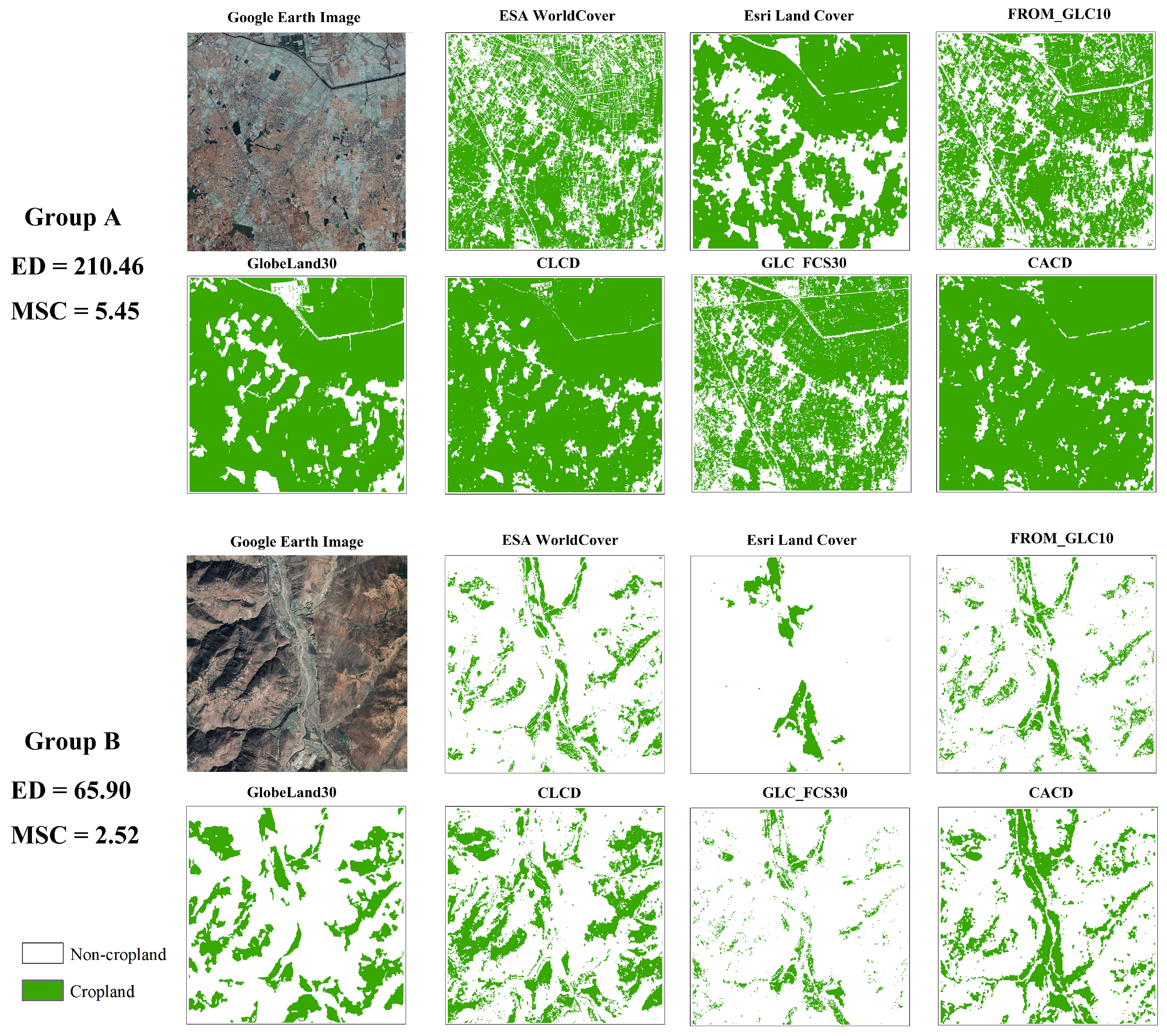
Figure 12. Visual verification of the positive correlation between edge density (ED) and Mean Spatial Consistency (MSC). Group A (High ED, High MSC): Represents intensive agricultural zones (e.g., basins, terraces) where high edge density is driven by dense internal linear features (ridges, roads). The strong, regular texture leads to high agreement among products. Group B (Low ED, Low MSC): Represents marginal mountainous areas where low edge density reflects sporadic, isolated cropland patches embedded in forests. These areas suffer from severe mixed pixel effects and omission errors, leading to low agreement.

Figure 12. Visual verification of the positive correlation between edge density (ED) and Mean Spatial Consistency (MSC). Group A (High ED, High MSC): Represents intensive agricultural zones (e.g., basins, terraces) where high edge density is driven by dense internal linear features (ridges, roads). The strong, regular texture leads to high agreement among products. Group B (Low ED, Low MSC): Represents marginal mountainous areas where low edge density reflects sporadic, isolated cropland patches embedded in forests. These areas suffer from severe mixed pixel effects and omission errors, leading to low agreement.

4.2. Region-Adaptive Mapping Strategies Based on Spatial Heterogeneity

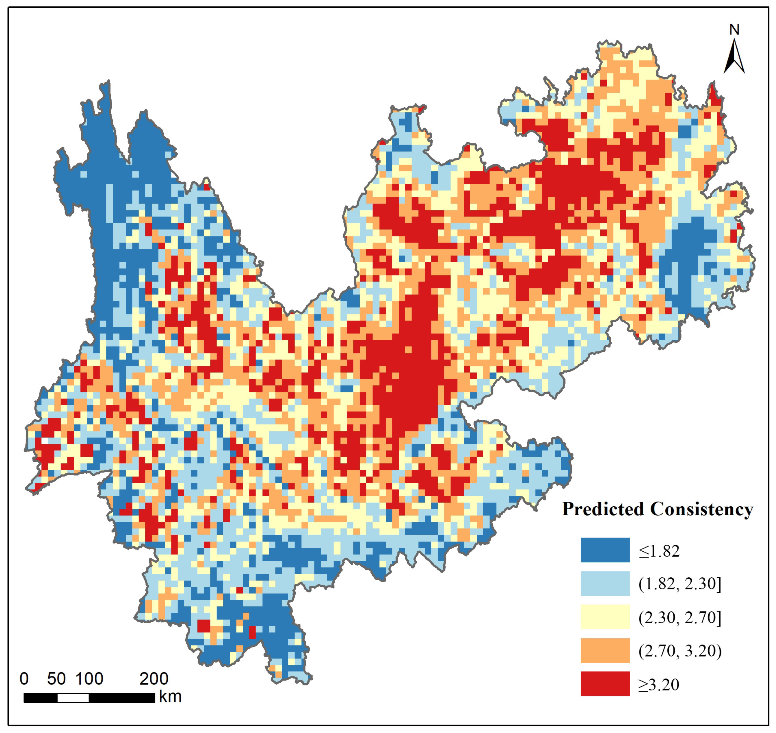
The spatial non-stationarity explicitly quantified by the MGWR model challenges the efficacy of traditional “one-size-fits-all” approaches for large-scale cropland mapping. By synthesizing the local regression coefficients, we mapped the spatial distribution of dominant driving factors (Figure 13) alongside the MGWR-predicted consistency (Figure 14). These visualizations reveal a fundamental divergence in mapping constraints: topographic distortion dictates the uncertainty in high-altitude gorges, whereas landscape fragmentation serves as the primary bottleneck in karst basins and transition zones.

Consequently, we advocate for a transition from monolithic algorithms to a region-adaptive mapping strategy. Future mapping efforts should adopt a spatially stratified framework where the study area is partitioned based on dominant drivers to apply targeted methodological interventions. More specifically, in topography-dominated zones, the workflow must prioritize signal restoration [26]; since standard optical correction often fails in severe shadow areas, integrating Synthetic Aperture Radar (SAR) (e.g., Sentinel-1) is critical to compensate for optical data gaps and geometric distortions in rugged terrain [56]. Conversely, in fragmentation-dominated areas constrained by landscape metrics (e.g., LPI, ED), the priority shifts to geometric precision. To mitigate the mixed pixel effect, strategies should incorporate Object-Based Image Analysis (OBIA) or deep learning architectures (e.g., U-Net), which treat the parcel rather than the pixel as the fundamental unit to reduce salt-and-pepper noise [57]. By allocating methodological resources to address these specific intrinsic difficulties, this targeted approach maximizes the overall cost-effectiveness and accuracy of regional mapping initiatives.

4.3. Implications for Product Selection Strategies

The diagnostic results from the MGWR analysis provide a physical basis for selecting appropriate cropland products in the YGP. Since the driving mechanisms (e.g., topography and fragmentation) exhibit significant spatial non-stationarity (Table 7 and Figure 11), a “one-size-fits-all” selection strategy is insufficient. Instead, we propose a region-adaptive selection framework based on the identified dominant constraints:

• Prioritizing Resolution in Fragmentation-Constrained Zones. Our results identify edge density (ED) as a ubiquitous global constraint and Mean Patch Size (MPS) as a significant positive driver of consistency. This confirms that the “mixed pixel effect” at patch boundaries is the primary source of uncertainty across the plateau. Recommendation: For static acreage inventory, particularly in karst basins dominated by small-holder farms, users should prioritize spatial resolution over spectral richness. Products with 10 m resolution (e.g., ESA WorldCover) are recommended to resolve the irregular boundaries of fragmented plots, thereby mitigating the omission errors inherent to coarser 30 m datasets.
• Adopting Data Fusion in Topography-Constrained Zones. The MGWR analysis reveals that mean slope exerts a strong, localized negative impact on consistency (∼72 km bandwidth), specifically in the high-altitude gorges of Western Yunnan. This indicates that topographic shadowing systematically degrades the performance of optical sensors in these specific sub-regions. Recommendation: In these rugged terrains, reliance on any single optical product is discouraged due to the risk of geometric distortion and shadowing. Future mapping or selection efforts should favor approaches that integrate Multi-Source Fusion (e.g., combining optical classifications with SAR data or DEM-based topographic correction) to compensate for the information loss in shadowed areas.
• Balancing Consistency for Long-term Monitoring. While human footprint (HFP) shows positive correlations in intensive agricultural zones, the localized negative influence of NDRI in karst border regions suggests spectral confusion between rocky desertification and fallow land. Recommendation: For change detection applications, spatial detail should be balanced with temporal stability. Users are advised to select products incorporating temporal consistency logic (e.g., CLCD) to filter out pseudo-changes caused by spectral ambiguity in rocky landscapes, ensuring that detected trends reflect genuine land cover conversion rather than noise.

4.4. Uncertainties and Limitations

While this study provides a comprehensive diagnosis of cropland mapping consistency, several uncertainties and limitations related to data availability and analytical design should be acknowledged.

A key limitation concerns spatial accuracy validation. Although visually interpreted samples were used to assess overall accuracy, their density was insufficient to construct spatially continuous accuracy surfaces for grid-scale analysis. Consequently, the local-scale analysis focused on consistency rather than absolute accuracy. At the county scale, statistical area comparison was adopted as a proxy for reliability; however, this aggregate indicator is subject to a cancellation effect, whereby commission and omission errors may offset each other and obscure local misclassification patterns.

Another source of uncertainty lies in the interpretation of consistency versus accuracy. Owing to these data constraints, the driving force analysis explains spatial disagreement among products rather than classification correctness. Consistency should not be equated with accuracy: high consistency does not guarantee correctness, and low consistency does not imply that all products are erroneous. Instead, low consistency reflects elevated mapping uncertainty and identifies regions where existing products fail to reach a consensus, highlighting areas that warrant methodological improvement.

Additional uncertainty arises from resolution discrepancies and aggregation effects. The cropland datasets employed differ in native spatial resolution (10–30 m). Although all products were resampled to a common resolution, residual sensor-related discrepancies remain. Furthermore, regarding the Modifiable Areal Unit Problem (MAUP), the MGWR analysis was conducted at an aggregated 10 km grid scale, while this choice inevitably introduces an averaging effect that smooths fine-scale landscape heterogeneity, it was explicitly adopted following the framework of Zou et al. [48] to minimize the estimate deviation triggered by spatial data homogeneity in complex terrains. This scale represents a necessary trade-off, prioritizing the detection of robust regional driving mechanisms over micro-scale spatial processes.

5. Conclusions

This study systematically evaluated the accuracy and spatial consistency of seven global land cover products in the heterogeneous karst landscapes of the YGP, employing an MGWR framework to disentangle the underlying physical constraints. The primary findings and implications are as follows:

1.

Product Accuracy and Recommendation. The comprehensive evaluation reveals a sharp polarization in product performance relative to the Third National Land Survey benchmark. Consequently, we identify the 10 m ESA WorldCover as the superior dataset specifically for fine-scale spatial pattern mapping and administrative-level area inventory. It achieved the highest spatial fidelity (OA = 0.81, F1-score = 0.72) by effectively resolving the mixed pixel dilemma in fragmented terrain. Simultaneously, at the county scale, it maintained optimal agreement with official statistical data ($R^2=0.84$), making it the most reliable baseline for static agricultural monitoring. In contrast, traditional products like GlobeLand30 and Esri Land Cover exhibited significant deviations (overestimation by ∼87.5% and omission by ∼42%, respectively), highlighting their limitations for these precision-demanding applications in complex karst environments.

2.

Scale-Dependent Impact Factors. The MGWR diagnostics provided novel insights into the spatial non-stationarity of error sources (adjusted $R^2=0.923$). We identified distinct driving mechanisms. Landscape fragmentation acts as a pervasive global constraint, showing a consistent negative correlation with accuracy across the plateau. This confirms that the highly fragmented cropping patterns characteristic of karst landforms are the primary source of uncertainty. Conversely, topographic slope operates as a dominant local constraint (bandwidth ∼72 km), with its inhibitory effect significantly intensifying in high-relief gorges where terrain shadowing and geometric distortion severely compromise optical remote sensing signals.

3.

Implications for Adaptive Mapping Strategies. To overcome these physical bottlenecks, future mapping efforts in karst regions must move beyond “one-size-fits-all” approaches. We propose a Region-Adaptive Mapping Strategy applicable to both static inventory (single-date) and dynamic monitoring (time-series). (1) Spatial Optimization for Inventory: In Topography-Constrained Zones, priority should be given to multi-source data fusion (e.g., integrating SAR) to compensate for shadow effects; in Fragmentation-Constrained Zones (typical of Karst basins), strategies should shift towards enhancing geometric precision using Object-Based Image Analysis (OBIA) or 10 m resolution data to capture small, irregular patch details. (2) Temporal Logic for Monitoring: While the above spatial strategies improve single-date accuracy, future time-series applications must further integrate temporal consistency algorithms (e.g., phenological stability checks) to suppress the pseudo-changes caused by spectral confusion in these complex terrains. This targeted approach provides a theoretical basis and practical pathway for improving the next generation of land cover products in ecologically fragile mountainous regions.

References

1. Foley, J.A.; Ramankutty, N.; Brauman, K.A.; Cassidy, E.S.; Gerber, J.S.; Johnston, M.; Mueller, N.D.; O’Connell, C.; Ray, D.K.; West, P.C.; et al. Solutions for a cultivated planet. Nature 2011, 478, 337–342. [Google Scholar] [CrossRef] [Scilit]
2. Potapov, P.; Turubanova, S.; Hansen, M.C.; Tyukavina, A.; Zalles, V.; Khan, A.; Song, X.P.; Pickens, A.; Shen, Q.; Cortez, J. Global maps of cropland extent and change show accelerated cropland expansion in the twenty-first century. Nat. Food 2022, 3, 19–28. [Google Scholar] [CrossRef] [Scilit]
3. Yu, Q.; Wu, W.; You, L.; Zhu, T.; van Vliet, J.; Verburg, P.H.; Liu, Z.; Li, Z.; Yang, P.; Zhou, Q.; et al. Assessing the harvested area gap in China. Agric. Syst. 2017, 153, 212–220. [Google Scholar] [CrossRef] [Scilit]
4. Weiss, M.; Jacob, F.; Duveiller, G. Remote sensing for agricultural applications: A meta-review. Remote Sens. Environ. 2020, 236, 111402. [Google Scholar] [CrossRef] [Scilit]
5. Gumma, M.K.; Thenkabail, P.S.; Teluguntla, P.G.; Oliphant, A.; Xiong, J.; Giri, C.; Pyla, V.; Dixit, S.; Whitbread, A.M. Agricultural cropland extent and areas of South Asia derived using Landsat satellite 30-m time-series big-data using random forest machine learning algorithms on the Google Earth Engine cloud. GISci. Remote Sens. 2020, 57, 302–322. [Google Scholar] [CrossRef] [Scilit]
6. Luo, K.; Moiwo, J.P. Rapid monitoring of abandoned farmland and information on regulation achievements of government based on remote sensing technology. Environ. Sci. Policy 2022, 132, 91–100. [Google Scholar] [CrossRef] [Scilit]
7. Chen, J.; Chen, J.; Liao, A.; Cao, X.; Chen, L.; Chen, X.; He, C.; Han, G.; Peng, S.; Lu, M.; et al. Global land cover mapping at 30 m resolution: A POK-based operational approach. ISPRS J. Photogramm. Remote Sens. 2015, 103, 7–27. [Google Scholar] [CrossRef] [Scilit]
8. Zanaga, D.; Van De Kerchove, R.; De Keersmaecker, W.; Souverijns, N.; Brockmann, C.; Quast, R.; Wevers, J.; Grosu, A.; Paccini, A.; Vergnaud, S.; et al. ESA WorldCover 10 m 2020 v100. 2021. Available online: https://zenodo.org/records/5571936 (accessed on 11 January 2026).
9. Yang, J.; Huang, X. The 30 m annual land cover dataset and its dynamics in China from 1990 to 2019. Earth Syst. Sci. Data 2021, 13, 3907–3925. [Google Scholar] [CrossRef] [Scilit]
10. Zhang, X.; Zhao, T.; Xu, H.; Liu, W.; Wang, J.; Chen, X.; Liu, L. GLC_FCS30D: The first global 30 m land-cover dynamics monitoring product with a fine classification system for the period from 1985 to 2022 generated using dense-time-series Landsat imagery and the continuous change-detection method. Earth Syst. Sci. Data 2024, 16, 1353–1381. [Google Scholar] [CrossRef] [Scilit]
11. Wang, J.; Yang, X.; Wang, Z.; Cheng, H.; Kang, J.; Tang, H.; Li, Y.; Bian, Z.; Bai, Z. Consistency analysis and accuracy assessment of three global ten-meter land cover products in rocky desertification region—A case study of Southwest China. ISPRS Int. J. Geo-Inf. 2022, 11, 202. [Google Scholar] [CrossRef] [Scilit]
12. WU, Z.; CAI, Z.; GUO, Y.; WANG, Y. Accuracy evaluation and consistency analysis of multi-source remote sensing land cover data in the Yellow River Basin. Chin. J. Eco-Agric. 2023, 31, 917–927. [Google Scholar]
13. Li, C.; Lei, L.; Jia, X.; Xiong, X.; Zhang, X. Accuracy and applicability assessment of vegetation types of the land cover products produced in China. Ecol. Indic. 2025, 174, 113506. [Google Scholar] [CrossRef] [Scilit]
14. Qiu, B.; Hu, X.; Chen, C.; Tang, Z.; Yang, P.; Zhu, X.; Yan, C.; Jian, Z. Maps of cropping patterns in China during 2015–2021. Sci. Data 2022, 9, 479. [Google Scholar] [CrossRef] [Scilit]
15. Cui, Y.; Liu, R.; Li, Z.; Zhang, C.; Song, X.P.; Yang, J.; Yu, L.; Chen, M.; Dong, J. Decoding the inconsistency of six cropland maps in China. Crop J. 2024, 12, 281–294. [Google Scholar] [CrossRef] [Scilit]
16. Shen, Y.; Zhang, X.; Yang, Z. Mapping corn and soybean phenometrics at field scales over the United States Corn Belt by fusing time series of Landsat 8 and Sentinel-2 data with VIIRS data. ISPRS J. Photogramm. Remote Sens. 2022, 186, 55–69. [Google Scholar] [CrossRef] [Scilit]
17. Naboureh, A.; Li, A.; Bian, J.; Moharrami, M.; Ebrahimy, H.; Lei, G.; Nan, X.; Zhang, Z.; Feizizadeh, B.; Dabove, P.; et al. Accuracies, discrepancies, and challenges of the 10 m global land cover products in mountains. GISci. Remote Sens. 2025, 62, 2556064. [Google Scholar] [CrossRef] [Scilit]
18. Lu, Y.; Li, L.; Dong, W.; Zheng, Y.; Zhang, X.; Zhang, J.; Wu, T.; Liu, M. A method for cropland layer extraction in complex scenes integrating edge features and semantic segmentation. Agriculture 2024, 14, 1553. [Google Scholar] [CrossRef] [Scilit]
19. Dai, Q.; Zhou, Z.; Huang, D.; Yang, Y.; Lu, H.; Li, Y. Response of land cover to multi-scale spatial effects in complex karst mountainous areas. Geocarto Int. 2025, 40, 2513520. [Google Scholar] [CrossRef] [Scilit]
20. Liu, P.; Pei, J.; Guo, H.; Tian, H.; Fang, H.; Wang, L. Evaluating the accuracy and spatial agreement of five global land cover datasets in the ecologically vulnerable south China Karst. Remote Sens. 2022, 14, 3090. [Google Scholar] [CrossRef] [Scilit]
21. Ji, X.; Han, X.; Zhu, X.; Huang, Y.; Song, Z.; Wang, J.; Zhou, M.; Wang, X. Comparison and validation of multiple medium-and high-resolution land cover products in Southwest China. Remote Sens. 2024, 16, 1111. [Google Scholar] [CrossRef] [Scilit]
22. Radwan, T.M.; Blackburn, G.A.; Whyatt, J.D.; Atkinson, P.M. Global land cover trajectories and transitions. Sci. Rep. 2021, 11, 12814. [Google Scholar] [CrossRef] [Scilit]
23. Qi, X.; Zhang, C.; Wang, K. Comparing remote sensing methods for monitoring karst rocky desertification at sub-pixel scales in a highly heterogeneous karst region. Sci. Rep. 2019, 9, 13368. [Google Scholar] [CrossRef] [Scilit] [PubMed]
24. Zhao, X.; Zhou, Z.; Wu, G.; Long, Y.; Luo, J.; Huang, X.; Chen, J.; Wu, T. High-resolution dynamic monitoring of rocky desertification of agricultural land based on spatio-temporal fusion. Land 2024, 13, 2173. [Google Scholar] [CrossRef] [Scilit]
25. Huang, D.; Zhou, Z.; Zhang, Z.; Dai, Q.; Lu, H.; Li, Y.; Huang, Y. Land Use/Land Cover Remote Sensing Classification in Complex Subtropical Karst Environments: Challenges, Methodological Review, and Research Frontiers. Appl. Sci. 2025, 15, 9641. [Google Scholar] [CrossRef] [Scilit]
26. Chen, R.; Yin, G.; Zhao, W.; Yan, K.; Wu, S.; Hao, D.; Liu, G. Topographic correction of optical remote sensing images in mountainous areas: A systematic review. IEEE Geosci. Remote Sens. Mag. 2023, 11, 125–145. [Google Scholar] [CrossRef] [Scilit]
27. He, S.; Shao, H.; Xian, W.; Yin, Z.; You, M.; Zhong, J.; Qi, J. Monitoring cropland abandonment in hilly areas with sentinel-1 and sentinel-2 timeseries. Remote Sens. 2022, 14, 3806. [Google Scholar] [CrossRef] [Scilit]
28. Ministry of Natural Resources of the People’s Republic of China. Land Survey Results Sharing and Application Service Platform. 2024. Available online: https://gtdc.mnr.gov.cn/ (accessed on 10 January 2026).
29. Zhang, S.; Xiong, K.; Qin, Y.; Min, X.; Xiao, J. Evolution and determinants of ecosystem services: Insights from South China karst. Ecol. Indic. 2021, 133, 108437. [Google Scholar] [CrossRef] [Scilit]
30. Ma, G.; Li, Q.; Yang, S.; Zhang, R.; Zhang, L.; Xiao, J.; Sun, G. Analysis of landscape pattern evolution and driving forces based on land-use changes: A case study of Yilong Lake watershed on Yunnan-Guizhou Plateau. Land 2022, 11, 1276. [Google Scholar] [CrossRef] [Scilit]
31. Zhang, X.; Liu, L.; Chen, X.; Gao, Y.; Xie, S.; Mi, J. GLC_FCS30: Global land-cover product with fine classification system at 30 m using time-series Landsat imagery. Earth Syst. Sci. Data 2021, 13, 2753–2776. [Google Scholar] [CrossRef] [Scilit]
32. Tu, Y.; Wu, S.; Chen, B.; Weng, Q.; Bai, Y.; Yang, J.; Yu, L.; Xu, B. A 30 m annual cropland dataset of China from 1986 to 2021. Earth Syst. Sci. Data 2024, 16, 2297–2316. [Google Scholar] [CrossRef] [Scilit]
33. Karra, K.; Kontgis, C.; Statman-Weil, Z.; Mazzariello, J.C.; Mathis, M.; Brumby, S.P. Global land use/land cover with Sentinel 2 and deep learning. In Proceedings of the 2021 IEEE International Geoscience and Remote Sensing Symposium IGARSS; IEEE: Piscataway, NJ, USA, 2021; pp. 4704–4707. [Google Scholar]
34. Gong, P.; Liu, H.; Zhang, M.; Li, C.; Wang, J.; Huang, H.; Clinton, N.; Ji, L.; Li, W.; Bai, Y.; et al. Stable classification with limited sample: Transferring a 30-m resolution sample set collected in 2015 to mapping 10-m resolution global land cover in 2017. Sci. Bull. 2019, 64, 370–373. [Google Scholar] [CrossRef] [Scilit]
35. Prudente, V.H.R.; Martins, V.S.; Vieira, D.C.; e Silva, N.R.d.F.; Adami, M.; Sanches, I.D. Limitations of cloud cover for optical remote sensing of agricultural areas across South America. Remote Sens. Appl. Soc. Environ. 2020, 20, 100414. [Google Scholar] [CrossRef] [Scilit]
36. Xu, P.; Tsendbazar, N.E.; Herold, M.; De Bruin, S.; Koopmans, M.; Birch, T.; Carter, S.; Fritz, S.; Lesiv, M.; Mazur, E.; et al. Comparative validation of recent 10 m-resolution global land cover maps. Remote Sens. Environ. 2024, 311, 114316. [Google Scholar] [CrossRef] [Scilit]
37. NASA JPL. NASADEM Merged DEM Global 1 arc second V001; NASA Land Processes Distributed Active Archive Center: Sioux Falls, South Dakota, 2020. [CrossRef]
38. Luo, Y.; Zhang, Z.; Chen, Y.; Li, Z.; Tao, F. ChinaCropPhen1km: A high-resolution crop phenological dataset for three staple crops in China during 2000–2015 based on leaf area index (LAI) products. Earth Syst. Sci. Data 2020, 12, 197–214. [Google Scholar] [CrossRef] [Scilit]
39. Mu, H.; Li, X.; Wen, Y.; Huang, J.; Du, P.; Su, W.; Miao, S.; Geng, M. A global record of annual terrestrial Human Footprint dataset from 2000 to 2018. Sci. Data 2022, 9, 176. [Google Scholar] [CrossRef] [Scilit]
40. Liu, J.; Zhou, Y.; Wang, J.; Pan, X.; Sun, R.; Bryan, B. Cropland Abandonment in China Dataset. 2025. Available online: https://figshare.com/articles/dataset/Cropland_Abandonment_in_China_Dataset/30466262/1 (accessed on 11 January 2026).
41. Vermote, E.; Wolfe, R. MODIS/Terra Surface Reflectance Daily L2G Global 1 km and 500 m SIN Grid V061; NASA Land Processes Distributed Active Archive Center: Sioux Falls, South Dakota, 2021. [CrossRef]
42. Wang, Y.; Tang, X.; Huang, Y.; Yang, J.; Lu, J. Identification and factor analysis of rocky desertification severity levels in large-scale karst areas based on deep learning image segmentation. Ecol. Indic. 2024, 167, 112565. [Google Scholar] [CrossRef] [Scilit]
43. Hesselbarth, M.H.; Sciaini, M.; With, K.A.; Wiegand, K.; Nowosad, J. landscapemetrics: An open-source R tool to calculate landscape metrics. Ecography 2019, 42, 1648–1657. [Google Scholar] [CrossRef] [Scilit]
44. Smith, J.H.; Stehman, S.V.; Wickham, J.D.; Yang, L. Effects of landscape characteristics on land-cover class accuracy. Remote Sens. Environ. 2003, 84, 342–349. [Google Scholar] [CrossRef] [Scilit]
45. Yuan, M.; He, G.; Wang, G.; Yin, R.; Zhang, Z.; Long, T.; Peng, Y. Spatial Consistency and Accuracy Assessment of Grassland Classification in the Sanjiangyuan Region: From Six Medium Resolution Land Cover Products. Remote Sens. 2025, 17, 3983. [Google Scholar] [CrossRef] [Scilit]
46. Song, Y.; Wang, J.; Ge, Y.; Xu, C. An optimal parameters-based geographical detector model enhances geographic characteristics of explanatory variables for spatial heterogeneity analysis: Cases with different types of spatial data. GISci. Remote Sens. 2020, 57, 593–610. [Google Scholar] [CrossRef] [Scilit]
47. Fotheringham, A.S.; Yang, W.; Kang, W. Multiscale geographically weighted regression (MGWR). Ann. Am. Assoc. Geogr. 2017, 107, 1247–1265. [Google Scholar] [CrossRef] [Scilit]
48. Zou, L.; Wang, J.; Bai, M. Assessing spatial–temporal heterogeneity of China’s landscape fragmentation in 1980–2020. Ecol. Indic. 2022, 136, 108654. [Google Scholar] [CrossRef] [Scilit]
49. Vanonckelen, S.; Lhermitte, S.; Van Rompaey, A. The effect of atmospheric and topographic correction methods on land cover classification accuracy. Int. J. Appl. Earth Obs. Geoinf. 2013, 24, 9–21. [Google Scholar] [CrossRef] [Scilit]
50. Congalton, R.G.; Gu, J.; Yadav, K.; Thenkabail, P.; Ozdogan, M. Global land cover mapping: A review and uncertainty analysis. Remote Sens. 2014, 6, 12070–12093. [Google Scholar] [CrossRef] [Scilit]
51. Shafizadeh-Moghadam, H.; Khazaei, M.; Alavipanah, S.K.; Weng, Q. Google Earth Engine for large-scale land use and land cover mapping: An object-based classification approach using spectral, textural and topographical factors. GISci. Remote Sens. 2021, 58, 914–928. [Google Scholar] [CrossRef] [Scilit]
52. Tonetti, V.; Pena, J.C.; Scarpelli, M.D.; Sugai, L.S.; Barros, F.M.; Anunciação, P.R.; Santos, P.M.; Tavares, A.L.; Ribeiro, M.C. Landscape heterogeneity: Concepts, quantification, challenges and future perspectives. Environ. Conserv. 2023, 50, 83–92. [Google Scholar] [CrossRef] [Scilit]
53. Islam, S.; Zhang, M.; Yang, H.; Ma, M. Assessing inconsistency in global land cover products and synthesis of studies on land use and land cover dynamics during 2001 to 2017 in the southeastern region of Bangladesh. J. Appl. Remote Sens. 2019, 13, 048501. [Google Scholar] [CrossRef] [Scilit]
54. Zhou, X.; Xie, X.; Xue, Y.; Xue, B. Ontology-based probabilistic estimation for assessing semantic similarity of land use/land cover classification systems. Land 2021, 10, 920. [Google Scholar] [CrossRef] [Scilit]
55. Wang, Y.; Xu, Y.; Xu, X.; Jiang, X.; Mo, Y.; Cui, H.; Zhu, S.; Wu, H. Evaluation of six global high-resolution global land cover products over China. Int. J. Digit. Earth 2024, 17, 2301673. [Google Scholar] [CrossRef] [Scilit]
56. Li, J.; Li, C.; Xu, W.; Feng, H.; Zhao, F.; Long, H.; Meng, Y.; Chen, W.; Yang, H.; Yang, G. Fusion of optical and SAR images based on deep learning to reconstruct vegetation NDVI time series in cloud-prone regions. Int. J. Appl. Earth Obs. Geoinf. 2022, 112, 102818. [Google Scholar] [CrossRef] [Scilit]
57. Gui, B.; Sam, L.; Bhardwaj, A.; Gómez, D.S.; Peñaloza, F.G.; Buchroithner, M.F.; Green, D.R. SAGRNet: A novel object-based graph convolutional neural network for diverse vegetation cover classification in remotely-sensed imagery. ISPRS J. Photogramm. Remote Sens. 2025, 227, 99–124. [Google Scholar] [CrossRef] [Scilit]
Figure 1. Geographical location of the study area (Yunnan and Guizhou Provinces) in Southwest China.
Land 15 00343 g001
Figure 2. Spatial distribution of cropland and non-cropland derived from seven land cover products in 2020.
Land 15 00343 g002
Figure 4. Scatter plots comparing the cropland area estimated by seven land cover products against the Third National Land Survey data across 217 county-level units in 2020. The red dashed line represents the 1:1 identity line, while the blue solid line indicates the linear regression fit.
Land 15 00343 g004
Figure 5. Spatial distribution of RE in cropland area estimation for seven land cover products at the county level in 2020.
Land 15 00343 g005
Figure 7. Spatial consistency analysis of cropland identification. (a) Spatial distribution of pixel-level consistency; (b) areal proportion of each consistency level; (c) average consistency scores aggregated to 10 km grid cells.
Land 15 00343 g007
Figure 8. Comparison of the explanatory power (q-statistic) of driving factors on cropland consistency at grid ( 10   km ) and county scales. Abbreviations: Topography: Elev. (elevation), Elev_SD (terrain relief), Slope (mean slope), Slope_SD (Slope Variability); Environment: Cloud (cloud frequency), NDRI (rocky desertification index), Pheno. Diff. (phenological heterogeneity); Landscape: PD (patch density), MPS (Mean Patch Size), AI (Aggregation Index), ED (edge density), LPI (Largest Patch Index); Anthropogenic: HFP (human footprint), Aband. Land (cropland abandonment).
Land 15 00343 g008
Figure 9. Interaction effects of driving factors on cropland consistency. The heatmaps display the interaction q-statistics between factor pairs at the (a) county scale and (b) grid scale ( 10   km ). Values on the diagonal represent single-factor q-statistics.
Land 15 00343 g009
Figure 10. Spatial distribution of local parameter estimates derived from the county-scale MGWR model.
Land 15 00343 g010
Figure 11. Spatial distribution of local parameter estimates and significance statistics derived from the grid-scale MGWR model.
Land 15 00343 g011
Figure 13. Spatial distribution of the primary driving factors affecting cropland mapping consistency.
Land 15 00343 g013
Figure 14. Spatial distribution of predicted consistency derived from MGWR.
Land 15 00343 g014