Spatiotemporal Dynamics and Driving Factors of the Urban Tourismification–Transportation Quality–Ecological Resilience System: A Case Study of 80 Cities in Central China

Abstract

Within China’s “Central China Rising” strategy, urban tourismification operates as a production mode that reconfigures spatial, economic, and ecological systems—mirroring global overtourism challenges seen in Barcelona and Venice, where rapid infrastructure development often prioritizes economic gains over ecological resilience (cf. Lines 43–46). This study examines 80 central Chinese cities (2010–2021), proposing the Urban Tourismification–Transportation Quality–Ecological Resilience System (UTTES) framework. Using entropy weighting, improved coupling coordination degree (CCD), GM (1,1) forecasting, and spatial Durbin models, we analyze coordination relationships, driving factors, and mechanisms. Key findings reveal the following: (1) UTTES coordination peaked in 2019 (pre-COVID), showing a spatial “center-periphery” gradient with provincial capitals leading. (2) Projections indicate transportation efficiency as a critical bottleneck—most cities will achieve good coordination post-2026. (3) Economic activity, social restructuring, and policy support drive the system, with spatial spillovers creating dual-path mechanisms (economic growth vs. manufacturing/environmental barriers). The UTTES framework advances a replicable methodology for diagnosing Tourism–Transportation–Ecology synergies in rapidly developing regions, integrating multidimensional indicators to balance environmental governance and tourism dynamics.

1. Introduction

Tourism functions as a powerful driver of sustainable development goals and plays a central role in urban growth globally [1]. However, the pervasive phenomenon of ‘overtourism,’ evident in heritage cities such as Barcelona and Venice, underscores the urgent need to reconcile tourism expansion with ecological preservation. Developing regions face analogous challenges, where rapid infrastructure development frequently prioritizes economic gains over ecological resilience. This dual dependency highlights that tourism is heavily reliant on the resources and environment of destination cities [2,3]. While nations like Costa Rica have strategically leveraged tourism as a conservation tool for rainforests and biodiversity, others, exemplified by Jakarta, experience significant tourism bottlenecks due to chronic traffic congestion, degrading accessibility to cultural sites and forcing itinerary modifications.

Urban planning, functionality, and governance increasingly align with the demands of tourismification—the process through which tourism activities reshape land use patterns, drive economic transitions, and evolve into a dominant lifestyle for residents and visitors [4,5,6,7]. Driven by the “people’s growing needs for a better life,” this global trend permeates residents’ daily lives and overall urban dynamics [8]. Manifestations range from residential conversion into guesthouses (e.g., Lijiang) to retail sector shifts towards tourism services (e.g., Paris, Lisbon), often conceptualized as tourism-led gentrification [9]. While tourismification stimulates digital transformation, urban restructuring, and economic upgrades, it concurrently generates significant negative externalities, including resource depletion, noise pollution, real estate overheating, and broader socio-ecological disruption [10]. Consequently, it acts as a core factor disrupting economic, social, cultural, and environmental dynamics [11].

Transportation serves as the essential infrastructure connecting cities and facilitating tourism. A well-developed system promotes regional resource flow, sharing, reduced energy consumption, and industrial optimization and enhances destination appeal and urban aesthetics [12]. Projects like the China–Pakistan Economic Corridor (CPEC) demonstrate its potential to boost tourism in regions like northern Pakistan [13,14]. However, the transportation sector also consumes approximately 10% of national energy and is a primary source of CO₂ emissions, posing significant environmental challenges [15]. The capacity to develop low-carbon systems varies considerably between economically advanced and less developed regions.

Rapid urbanization has inflicted irreversible damage on urban ecosystems, elevating the importance of ecological resilience—defined as a system’s capacity to absorb disturbances while maintaining essential functions, structure, identity, and feedback mechanisms [16]. This concept underpins global urban management initiatives like the Rockefeller Foundation’s “100 Resilient Cities” [17] and is a crucial indicator of overall urban resilience [18]. Ecological resilience ensures ecosystems maintain balance against short-term fluctuations, preventing overexploitation, preserving carrying capacity, and underpinning ecological civilization [19,20,21,22]. Sustainable tourism can enhance this resilience [23], yet urban development, particularly transport expansion, often negatively impacts fragile ecosystems [24]. Enhancing urban ecological resilience is, therefore, critical for mitigating urbanization challenges and achieving ecological security and sustainable development.

Global urbanization intensifies the interdependence between socioeconomic development, infrastructure demands (especially transport), and environmental sustainability. Tourismification—the systemic transformation of cities into tourism-oriented economies—exerts unprecedented pressure on transport networks and ecological boundaries, challenging urban livability worldwide [25,26,27]. While prior research has examined urban subsystems, including resource–environment–urbanization linkages, economic–resource-energy–environment interactions [28,29], and economic–social–environment synergies [30,31], the integrated dynamics governing the triad of Urban Tourismification, Transport Efficiency, and Ecological Resilience (UTTES) remain critically underexplored [32]. This gap impedes the holistic governance of sustainable cities amid escalating climate vulnerabilities and tourism-driven urbanization.

Current understanding is constrained by three key limitations: (1) A deficiency in integrated analysis, where tourismification–transport–ecology interactions are rarely examined as an interconnected triad; (2) temporal oversights in conventional coupling coordination degree (CCD) models, neglecting subsystem developmental disparities and time-lag effects; and (3) methodological constraints in quantifying tourismification’s integration within sustainability frameworks, with spatial drivers of UTTES coordination unaddressed.

To address these critical gaps, this study proposes the Urban Tourismification–Transportation Quality–Ecological Resilience System (UTTES) framework. It hypothesizes that synergistic UTTES development achieves dynamic equilibrium among tourismification’s growth momentum, transport efficiency’s spatial capacity, and ecological resilience’s safety boundaries. Consequently, the research investigates the following questions:

• How do tourismification, transport efficiency, and ecological resilience co-evolve spatiotemporally;
• Which socioeconomic drivers (economic activity, social restructuring, policy support) govern UTTES coordination;
• Does synergistic UTTES development balance tourism growth, transport capacity, and ecological thresholds?

The primary objectives are as follows:

(1)

Operationalize tourismification metrics within the UTTES framework;

(2)

Deploy an improved CCD model incorporating a time dynamic coefficient to diagnose spatiotemporal evolution patterns and temporal disequilibrium among subsystems;

(3)

Identify spatial drivers through advanced econometric analysis.

Theoretically, this study advances complex systems discourse by integrating tourismification into urban resilience paradigms. Methodologically, it innovates through time-sensitive CCD modeling. Empirically, it provides evidence for Tourism–Transport–Ecology governance.

The remainder of this article is structured as follows: Section 2 synthesizes the conceptual and empirical foundations of UTTES linkages. Section 3 details the indicator system, the improved CCD methodology, and spatial econometric approaches. Section 4 presents the spatial–temporal evolution results. Section 5 discusses the theoretical and policy implications through a comparison of the literature. Section 6 concludes with governance insights and research limitations.

2. Literature Review

2.1. Foundational Concepts of UTTES: Interdependencies in Complex Urban Systems

Urban sustainability is increasingly analyzed through complex systems theory, where nonlinear interactions among socio-ecological and economic subsystems generate emergent behaviors. This perspective frames cities as complex adaptive systems, underpinning frameworks like resource–environment–urbanization [25,26,27], economy–resource–energy–environment [28,29], and economy–society–environment couplings [30,31]. Within this context, the Urban Tourism–Transport–Ecology System (UTTES) emerges as a critical nexus demanding integrated analysis.

Central to UTTES is urban tourismification, a transformative process reshaping land use patterns (e.g., commercial/residential conversion), driving economic transitions towards service-oriented economies, and evolving into a dominant lifestyle [7]. Sequera conceptualizes this as tourism-led gentrification [9], exemplified by residential conversion into guesthouses (e.g., Lijiang) and retail shifts towards tourism services (e.g., Paris, Lisbon). While enabling economic upgrading, tourismification imposes significant burdens, including resource depletion, noise pollution, real estate overheating, and broader socio-ecological disruption.

Transportation serves as both the essential enabler and a major environmental stressor within UTTES. It underpins tourism accessibility and catalyzes regional development, as seen with projects like the China–Pakistan Economic Corridor (CPEC) boosting tourism in regions like northern Pakistan [11,12]. However, the sector consumes approximately 10% of national energy and is a primary source of CO₂ emissions, degrading urban air quality [33,34]. Although innovations like electric vehicles and shared micro-mobility offer mitigation pathways [35,36], their adoption remains uneven globally.

Consequently, ecological resilience—defined as the capacity of ecosystems to absorb disturbances while retaining essential functions and structures—becomes imperative for urban sustainability, underpinning initiatives like “100 Resilient Cities”. While sustainable tourism practices can theoretically enhance resilience, the combined pressures of tourismification and associated transport infrastructure expansion often fragment habitats, degrade ecosystem services, and threaten biodiversity, undermining the long-term resilience upon which sustainability depends.

2.2. UTTES Subsystem Interdependencies and Coordinated Development Drivers

The UTTES framework reveals intricate, dynamic feedback loops among its core subsystems (Figure 1), highlighting profound interdependence. Tourismification fundamentally relies on transport resources (accessibility, capacity) while exerting direct pressures on urban ecology through land conversion, waste, and resource consumption [37]. Conversely, enhanced transport accessibility accelerates tourismification, fueling visitor influxes and facilitating spatial–economic transformations [38,39]. Simultaneously, the state of ecological resilience imposes critical biophysical constraints on the scale and intensity of both tourismification and transport expansion; degraded ecosystems possess diminished capacity to support these activities sustainably [40].

These interdependencies are modulated by complex socioeconomic and institutional factors: Economic Drivers: Scale of activity (GDP), foreign direct investment (FDI), and financial market maturity shape investment in tourism and transport infrastructure [41]. Socio-structural Drivers: Urbanization rates, demographic shifts, and industrial composition (especially service vs. primary/secondary balance) [42,43,44] influence demand for tourism/transport and socio-ecological vulnerability. Policy and Governance Drivers: Stringency of environmental regulations, government expenditure on sustainability, and strategic spatial planning play a decisive role in mitigating externalities or exacerbating conflicts [45].

While existing research delineates UTTES components and bilateral interactions, a significant gap persists. Prior studies neglect the comprehensive spatiotemporal analysis of the synergistic/antagonistic relationships binding the tourism, transport, and ecology subsystems across scales and time. Furthermore, robust methodological tools specifically designed to quantify tourismification’s role as a primary coupling mechanism influencing transport–ecology dynamics within the integrated UTTES framework are critically lacking. Addressing these gaps is essential for developing effective policies for coordinated UTTES development.

2.3. Methodological Foundations for Complex System Analysis

The quantification of coupling coordination in complex systems requires multidimensional analytical approaches. The coupling coordination degree (CCD) model serves as the core framework for evaluating synergistic effects between subsystems [46], though its classical formulation often neglects temporal dynamics. Recent methodological advances address this through dynamic time coefficients that capture lag effects [47]. For objective weight determination, three complementary techniques are widely adopted:

The entropy weight method is an objective weighting technique based on information entropy, measuring data disorder to reflect informational utility. Higher entropy indicates greater variability and decision significance. The entropy weight method (EWM) quantifies information uncertainty through probability distributions [48]:

$${\mathrm{e}}_i=-k\sum p_{ij}\ln \left(p_{ij}\right)$$

The coefficient of variation (CV) measures the relative dispersion of indicators [49]. It is used to evaluate indicator volatility through deviation from the mean, prioritizing high-fluctuation indicators [47]:

$${\sigma }_i\sqrt{{\displaystyle \frac{1}{n}}\sum {\left(x_{ij}-E_i\right)}^2}$$

Mean squared deviation (MSD) evaluates contribution through fluctuation amplitude [50]. It standardizes variability by dividing the standard deviation by the mean, enabling cross-dataset comparisons [48]:

$$\widehat{f}\left(x\right)={\displaystyle \frac{1}{nh}}\sum k\left({\displaystyle \frac{x-x_i}{h}}\right)$$

The spatiotemporal analysis employs the following:

The kernel density estimation (KDE) is used to visualize distribution dynamics using nonparametric smoothing [51]. It non-parametrically estimates probability density distributions using kernel functions (e.g., Gaussian), revealing spatial/temporal clustering patterns [49]:

$$I={\displaystyle \frac{n}{\sum W_{ij}}}{\displaystyle \frac{\sum W_{ij}\left(x_i-\overline{x}\right)\left(x_j-\overline{x}\right)}{\sum {\left(x_i-\overline{x}\right)}^2}}$$

Gi statistic identifies local hotspots:

$$G_i^{*}={\displaystyle \frac{\sum W_{ij}\left(d\right)x_j}{\sum x_j}}$$

It quantifies spatial dependence via Moran’s I (global clustering) and Getis-Ord (Gi*) (local hotspots), where (I > 0) indicates clustering, and (I < 0) indicates dispersion.

For limited-data forecasting, the Grey Model (GM) (1,1) utilizes Accumulated Generating Operations (AGO) to extract system trends [52]. It forecasts short-term trends with limited data via Accumulated Generating Operations (AGO), reducing randomness without distributional assumptions [50]:

$${\displaystyle \frac{d{x}_1}{dt}}+a{x}_1=u$$

The following parameters are estimated by least squares:

$$\widehat{a}={\left(B^{T}B\right)}^{-1}{B}^T{y}_n$$

These methods underpin the coupling coordination degree (CCD) model for quantifying subsystem synergies [53]. Classical CCD models, however, often neglect temporal dynamics—a limitation addressed by time-adjusted CCD extensions incorporating lag effects [52]. Integrating these tools enables robust spatiotemporal analysis of UTTES synergies, addressing critical gaps in tourismification–transport–ecology nexus research.

3. Materials and Methods

3.1. Research Design and Study Area

3.1.1. Research Design

The research design is depicted in Figure 2. This study is conducted in three sequential stages. Stage 1: UTTES System Assessment. An evaluation framework is first established based on the literature. Subsequently, spatiotemporal analysis is performed using an improved coupling coordination degree (CCD) model incorporating dynamic time coefficients to assess interactions among subsystems. Geographic patterns are characterized through kernel density estimation (KDE) and spatial autocorrelation analysis (employing Global Moran’s I and local Gi* statistics). Future trends are forecasted using the GM (1,1) model. Stage 2: Driving Factor Analysis. Indicators across three dimensions—economic activity levels, social structural transformation, and policy support strength—are selected to quantify their influences on UTTES coordination. Stage 3: Policy Recommendations. Based on the findings, evidence-based strategies are proposed to promote sustainable urban development in central China.

3.1.2. Study Area

According to the MasterCard Global Destination Cities Index report, prior to the pandemic, China had risen to become the second-largest source country among the 200 global tourism destinations [54]. Within this context, the rise of the central region holds significant importance for China’s goal of fully realizing a moderately prosperous society. However, despite being one of the four major economic regions (eastern, central, western, and northeastern), the central region has consistently faced the issue of “central region collapse”(Figure 3). On the demand side, accelerating urbanization and the development of urban agglomerations are primary pathways for promoting the rise of the central region. However, due to the vast geographical span and inconsistent statistical criteria across the region, data collection is complex and cumbersome, making quantitative analysis a major challenge in studies of the central region. On the supply side, cities in the central region are rich in tourism resources. For instance, Western Hunan and Southern Jiangxi have been designated as national-level cultural and tourism demonstration zones, receiving special financial support. Emerging industries, such as the “night economy” in Changsha and industrial tourism in Wuhan, have also gained significant momentum. However, cities in the central region continue to face challenges, such as product homogenization, excessive reliance on ticket-based economies, and pressures from ecological carrying capacity. Therefore, the coordinated development of the UTTES system in this region remains an area requiring further investigation. The demand and supply dynamics outlined above provide strong justification for selecting case study cities in this research. As a result, this study includes 80 prefecture-level cities from the central region for analysis.

Table 1. Tourism-related data from the six central provinces in 2019.

Province	Number of 5A-Level Scenic Spots (Count)	Total Number of Tourists (Hundreds of Millions)	Total Tourism Revenue (Hundreds of Millions of Yuan)	Travel Agencies	Star-Rated Hotels
Shanxi	8	8.3	8026.9	927	190
Henan	14	10	7700	1156	361
Anhui	11	8.2	8510	1487	268
Hubei	12	6	6927.38	1267	330
Hunan	9	8.3	1057.8	1143	302
Jiangxi	12	7.9	9656.38	909	310

presents the basic information of the study area.

3.2. Indicator System and Data Sources

This study includes three subsystems: urban tourismification, transportation efficiency, and ecological resilience.

Urban tourismification is constructed from three dimensions: tourism supply, tourism development, and tourism industry [55]. Supply tourismification refers to the capacity of urban tourist attractions, travel agencies, and star-rated hotels to accommodate visitors. Development tourismification measures the quality and potential of urban tourism consumption, which is also an important aspect of the city’s tourism atmosphere and residents’ quality of life. Industry tourismification measures the direct contribution of tourism to the total urban economy, encompassing economic benefits generated by various tourism-related sectors such as accommodation, transportation, sightseeing, shopping, and entertainment, thus highlighting the position of tourism in the urban economic structure and the overall competitiveness of the urban tourism industry.

Transportation efficiency includes regional connectivity systems and internal urban systems. Due to geographical constraints, the central regions of Shanxi and Henan, reliant on the middle section of the Yellow River, have poor navigability, limiting their potential [56]. Moreover, there are only nine inland ports in the central region, with a low representation and insufficient capacity for quantification. Therefore, water transportation efficiency is excluded from the UTTES model. Additionally, existing measures of transportation efficiency lack a comprehensive understanding of internal urban transportation systems. As such, regional connectivity systems encompass rail, air, and road conditions, while internal systems include urban road conditions and public transportation networks. A well-rounded transportation system can better support the phenomenon of tourismification. A good transportation system reduces travel time for incoming tourists, allowing them to visit more attractions and expand the scope of recreational activities within limited time [2], thus contributing to the multiplier effects of tourism.

Ecological resilience refers to the capacity of ecosystems to resist, recover from, and transform in response to disturbances, encompassing three key dimensions: resistance, recovery, and transformation [19]. It is closely related to ecological recovery capacity, which reflects an ecosystem’s ability to withstand environmental pressures, such as pollution, and restore itself through management and restoration practices [57]. The Pressure–State–Response (PSR) model, proposed by the United Nations Environment Program (UNEP), defines urban ecological resilience as the result of the interaction between external pressures, the current state of the ecosystem, and societal responses to environmental stressors [58]. This holistic perspective emphasizes that ecosystems are not only influenced by production and consumption patterns but also depend on their inherent capacity to maintain ecological functions [59]. Given data limitations, current indicators for measuring resilience focus on quantifiable environmental parameters, such as air and water quality, biodiversity, and soil health [60]. While ecological resilience is critical for enhancing ecosystem sustainability and adapting to climate change, ongoing research is needed to refine these indicators and improve our ability to assess and manage ecological resilience, particularly in rapidly urbanizing areas [61].

The ecological resilience subsystem is based on the concept of ecological recovery capacity [22]. Ecological recovery capacity reflects the ability of the ecosystem to resist, recover, and transform. Therefore, it includes three criteria: pollution production, pollution management, and ecological restoration. The Pressure–State–Response (PSR) model, developed by the United Nations Environment Program, suggests that urban ecological resilience is the result of the interaction between pressure, state, and response. Consequently, some scholars attempt to construct ecological resilience systems based on these three dimensions. This study agrees with the perspective that “ecosystems are not only related to production and consumption patterns but also depend on their maintaining capacity.”

The availability of comprehensive indicators and existing literature on driving factors is used to select the driving factors from three perspectives: economic activity level, social structure transformation, and policy support strength [62,63,64]. Economic activity level includes GDP per capita, financial sector development, and foreign investment intensity. Social structure transformation considers urbanization level, manufacturing sector ratio, and service sector ratio. Policy support strength includes the strength of environmental regulations and government support levels.

Data for

Table 2. UTTES evaluation indicator system and combined weights.

Subsystems	Criterion Layer	Index Layer and Direction	Units	Combined Weights	Reference
Urban Tourismification	Supply Tourismification	$X_1$: Attraction capacity	10,000 visitors per site	0.1273	[55]
		$X_2$: Travel agency capacity	10,000 visitors per agency	0.1305	[55]
		$X_3$: Star-rated hotel capacity	10,000 visitors per hotel	0.1456	[55]
	Development Tourismification	$X_4$: Per capita tourism income of urban residents	Billion CNY per 10,000 people	0.1735	[2]
		$X_5$: Per capita tourism visits of urban residents	10,000 visits per capita	0.1619	[64]
	Industry Tourismification	$X_6$: Tourism industry contribution	Billion CNY	0.1282	[64]
		$X_7$: Tourism industry agglomeration level	Billion CNY	0.133	[64]
Transportation Efficiency	Rail Efficiency	$X_8$: Train station density	Stations per km2	0.0533	[2,56]
		$X_9$: Train stops per capita	Train stops per 10,000 people	0.0644	[2,56]
	Air Efficiency	$X_{10}$: Flight operation status	Number of aircraft	0.1226	[2,56]
		$X_{11}$: Airport density	m2 per km2	0.1246	[2,56]
	Road Efficiency	$X_{12}$: Per capita number of private cars	Cars per 10,000 people	0.084	[2,56]
		$X_{13}$: Road density	km per km2	0.0554	[2,56]
	Urban Roads Efficiency	$X_{14}$: Per capita urban road area	m2	0.0609	[2,56]
		$X_{15}$: Per capita sidewalk area	10,000 m2 per 10,000 people	0.0893	[2,56]
		$X_{16}$: Interchange bridges	Number	0.08	[2,56]
	Urban Transport Efficiency	$X_{17}$: Per capita public transport vehicles	Vehicles per 10,000 people	0.0785	[2,56]
		$X_{18}$: Per capita taxi fleet	Vehicles per 10,000 people	0.0843	[2,56]
		$X_{19}$: Rail track length	km	0.1027	[2,56]
Ecological Resilience	Pollution Production	$X_{20}$: Industrial wastewater discharge	10,000 tons	0.084	[19,22]
		$X_{21}$: Sulfur dioxide emissions	tons	0.0662	[19,22]
		$X_{22}$: Nitrogen oxide emissions	tons	0.1061	[22,57]
		$X_{23}$: Industrial dust emissions	tons	0.0118	[22,57]
	Pollution Management	$X_{24}$: Total sewage treatment volume	10,000 m3	0.1183	[22,58]
		$X_{25}$: Municipal waste collection volume	10,000 tons	0.1274	[22,59]
		$X_{26}$: Industrial dust removal	tons	0.0695	[22,59]
	Ecological Restoration	$X_{27}$: Per capita total water resources	10,000 m3 per 10,000 people	0.0924	[59,60]
		$X_{28}$: Per capita green space	hectares per 10,000 people	0.1293	[60,61]
		$X_{29}$: Number of days with air quality above secondary standard	days	0.1522	[61]
		$X_{30}$: Traffic Noise Average	decibels	0.0428	[22]

and

Table 3. Driving factor indicator system.

Driving Layer	Driving Factor	Index Description
Economic activity levels	Economic Development Level	Per capita GDP
	Financial Sector Development	Total deposits and loans of financial institutions/GDP
	Foreign Investment Intensity	Actual use of foreign capital
Social structural transformation	Urbanization Level	Urban population/total population
	Manufacturing Sector Ratio	Share of secondary industry in total economy
	Service Sector Ratio	Share of tertiary industry in total economy
Policy support strength	Environmental Regulation Strength	Local GDP/total pollution emissions
	Government Support Level	Local government general budget expenditure

were compiled by the researchers, with training data sourced from the 114 Ticketing Network, 911 Query Network, 12306 website, and other ticketing platforms. Civil aviation data comes from the Civil Aviation Airport Production Statistics Bulletin and the National Airport Information Overview. Other data were sourced from the “China Urban Construction Statistical Yearbook” (2010–2019), “City Statistical Yearbook,” “China Tertiary Industry Statistical Yearbook,” “China Transportation Yearbook,” and local-level city statistics bulletins.

3.3. Methodology

Methodological framework illustrating the analytical workflow is shown in Figure 4. The improved coupling coordination degree (CCD) model with dynamic time coefficient serves as the core analytical engine, feeding three parallel analysis streams: (1) spatiotemporal evolution analysis with kernel density estimation and spatial autocorrelation, (2) future trend prediction using the Grey Model GM (1,1), and (3) driving factor analysis through econometric modeling. All analytical outputs converge to inform policy recommendations.

3.3.1. Combination Weight

To eliminate the influence of subjective factors and extreme values on the 80 prefecture-level cities, this study employs three weighting methods to calculate the combined weight $w_i$ of the 30 indicators.

3.3.2. Combination Weight Calculation

Three objective methods—EWM, MSD, and CV—compute combined weights ($w_i$) for 30 indicators (Table 2):

• Normalize raw data.

$$x_{ij}=\left\{\begin{array}{c}{\displaystyle \frac{X_{ij}-X_i^{\min }}{X_i^{\max }-X_i^{\min }}} if positive indicator\\ {\displaystyle \frac{X_i^{\max }-X_{ij}}{X_i^{\max }-X_i^{\min }}} if negative indicator\end{array}\right.$$

2.

Calculate weights via EWM, MSD, and CV in detail:

Entropy weight method (EWM) calculates weights via information entropy ($e_i$), where higher entropy indicates greater indicator significance (Equations (1)–(5)).

$$p_{ij}={\displaystyle \frac{x_{ij}}{{\sum }_{j=1}^n{x}_{ij}}}$$

(1)

$$k={\displaystyle \frac{1}{\ln \left(n\right)}}$$

(2)

$$e_i=-k\sum _{j=1}^n{p}_{ij}\ln \left(p_{ij}\right)$$

(3)

$$d_i=1-e_i$$

(4)

$$w_i={\displaystyle \frac{d_i}{{\sum }_{i=1}^m{d}_i}}$$

(5)

Mean squared deviation (MSD) assigns weights based on data volatility $\left({\mathsf{\sigma }}_{\mathrm{i}}\right)$ (Equations (6)–(8)).

$$E_i={\displaystyle \frac{1}{n}}\sum _{j=1}^n{x}_{ij}$$

(6)

$${\mathsf{\sigma }}_i=\sqrt{{\displaystyle \frac{1}{n}}\sum _{j=1}^n{\left(x_{ij}-E_i\right)}^2}$$

(7)

$$w_i={\displaystyle \frac{{\mathsf{\sigma }}_i}{{\sum }_{i=1}^m{\mathsf{\sigma }}_i}}$$

(8)

Coefficient of variation (CV) normalizes weights by relative variability $\left({\mathrm{v}}_{\mathrm{i}}\right)$ (Equations (9) and (10)).

$$v_i={\displaystyle \frac{{\mathsf{\sigma }}_i}{\overline{x_i}}}$$

(9)

$$w_i={\displaystyle \frac{v_i}{{\sum }_{i=1}^m{v}_i}}$$

(10)

3.

Derive final weight $\left({\mathrm{w}}_{\mathrm{i}}\right)$ as the arithmetic mean.

3.3.3. Improved CCD Model

To address temporal lags in traditional CCD, a dynamic coefficient F measures inter-period changes:

Computer growth rate.

$$f_{ij}={\displaystyle \frac{{\overline{x}}_{ij}-{\overline{x}}_{i\left(j-1\right)}}{{\overline{x}}_{i\left(j-1\right)}}}$$

(11)

Derive time-adjustment coefficient.

$$F=\sum _{j=j_{\min }}^{j_{\max }}\left(\sum _{i=1}^m{w}_i{f}_{ij}\right)$$

(12)

Subsystem indices $\left({\mathrm{T}}_{\mathsf{\mu }}^{\mathrm{*}}\right)$ and coordination degree $\left({\mathrm{D}}^{\mathrm{*}}\right)$ are calculated as follows:

Adjust subsystem score.

$$T_{\mathsf{\mu }}^{*}=T_{\mathsf{\mu }}\cdot {\left(1-F\right)}^{j_{\max }-j}$$

(13)

Calculate interaction-adjusted coupling.

$$C^{*}=\sqrt{\left[1-\sum _{a>b,b=1}^u\sqrt{{\displaystyle \frac{{\left(T_a^{*}-T_b^{*}\right)}^2}{{\sum }_{r=1}^{u-1}r}}}\right]\cdot {\left(\prod _{a=1}^u{\displaystyle \frac{T_a^{*}}{\max T_a^{*}}}\right)}^{{\displaystyle \frac{1}{u-1}}}}$$

(14)

Coordination types are classified by $\left({\mathrm{D}}^{\mathrm{*}}\right)$ thresholds (

Table 4. Types of coordinated development.

The Relationship Among Variables	Status
$T_{tourismification}^{*}>T_{transportation}^{*}, T_{tourismification}^{*}>T_{ecology}^{*}$	Advancing tourismification
$T_{transportation}^{*}>T_{tourismification}^{*}, T_{transportation}^{*}>T_{ecology}^{*}$	Advancing transportation quality
$T_{ecology}^{*}>T_{tourismification}^{*}, T_{transportation}^{*}>T_{ecology}^{*}$	Advancing ecological resilience
$T_{transportation}^{*}>T_{tourismification}^{*}, T_{ecology}^{*}>T_{tourismification}^{*}$	Lagging tourismification
$T_{tourismification}^{*}>T_{transportation}^{*}, T_{ecology}^{*}>T_{transportation}^{*}$	Lagging transportation efficiency
$T_{tourismification}^{*}>T_{ecology}^{*}, T_{transportation}^{*}>T_{ecology}^{*}$	Lagging ecological resilience

and

Table 5. Classification of the CCD.

Coordination Phase	Coordination Degree	Coupling Coordination Type
Efficient coordination (0.7 < D ≤ 1)	0.9 < D ≤ 1	Quality coordination
	0.8 < D ≤ 0.9	Good coordination
	0.7 < D ≤ 0.8	Intermediate coordination
Basic coordination (0.4 < D ≤ 0.7)	0.6 < D ≤ 0.7	Moderate coordination
	0.5 < D ≤ 0.6	Mild coordination
	0.4 < D ≤ 0.5	Barely coordination
Maladjustment (0 ≤ D ≤ 0.4)	0.3 < D ≤ 0.4	Mild imbalance
	0.2 < D ≤ 0.3	High imbalance
	0.1 < D ≤ 0.2	Serious imbalance
	0 ≤ D ≤ 0.1	Extreme imbalance

):

$$D^{*}=\sqrt{C^{*}\cdot T^{*}}$$

(15)

3.3.4. Spatial–Temporal Analysis

Kernel density estimation (KDE) smooths UTTES distributions using a Gaussian kernel (Equation (16)), bandwidth (h) optimized via Silverman’s rule:

$$\widehat{f}\left(x\right)={\displaystyle \frac{1}{nh}}\sum _{i=1}^{n}K\left({\displaystyle \frac{x-X_i}{h}}\right)$$

(16)

3.3.5. GM (1,1) Model

Forecast via AGO and least-squares fitting (Equations (17)–(23)). The procedure is as follows:

Accumulated Generating Operation (AGO) on raw sequence ${\mathrm{x}}_0$ (Equation (17)).

$$x_0=\{x_0\left(1\right),x_0\left(2\right),\dots ,x_0\left(n\right)\}$$

(17)

$$x_1=\{x_1\left(1\right),x_1\left(2\right),\dots ,x_1\left(n\right)\}$$

(18)

$${\displaystyle \frac{d{x}_1}{dt}}+a{x}_1=u$$

(19)

Solve grey differential equation (Equation (19)) via least squares (Equations (20)–(22)).

$$B=\left[\begin{array}{ccc}-{\displaystyle \frac{1}{2}}\left[x_1\left(1\right)+x_1\left(2\right)\right]& \dots & 1\\ ⋮& \ddots & ⋮\\ -{\displaystyle \frac{1}{2}}\left[x_1\left(n-1\right)+x_1\left(n\right)\right]& \dots & 1\end{array}\right]$$

(20)

$$y_n={\left[x_0\left(2\right),x_0\left(3\right),\dots ,x_0\left(n\right)\right]}^T$$

(21)

$$\widehat{a}={\left[a\hspace{1em}u\right]}^T={\left(B^{T}B\right)}^{-1}{B}^T{y}_n$$

(22)

Generate predictions $\left(\widehat{{\mathrm{x}}_1}\left(\mathrm{k}+1\right)\right)$ (Equation (23)).

$$\widehat{x_1}\left(k+1\right)=\left(x_0\left(1\right)-{\displaystyle \frac{u}{a}}\right)e^{-ak}+{\displaystyle \frac{u}{a}},\left(k=\mathrm{1,2},\dots ,n\right)$$

(23)

3.3.6. Spatial Models:

• Spatial Autocorrelation

Compute global Moran’s I (Equation (24)) and local $\left(G_i^{*}\right)$ (Equation (25)) to detect CCD clustering. Spatial weight $\left(W_{ij}\right)$ uses inverse Euclidean distance.

Spatial autocorrelation uses Moran’s I for global clustering and $\left(G_i^{\mathrm{*}}\right)$ for local hotspots:

$$I={\displaystyle \frac{n}{{\sum }_{i=1}^n{\sum }_{j=1}^n{w}_{ij}}}\cdot {\displaystyle \frac{{\sum }_{i=1}^n{\sum }_{j=1}^n{w}_{ij}\left(x_i-\overline{x}\right)\left(x_j-\overline{x}\right)}{{\sum }_{i=1}^n{\left(x_i-\overline{x}\right)}^2}}$$

(24)

$$G_i^{*}={\displaystyle \frac{{\sum }_{j=1}^n{w}_{ij}\left(d\right)x_j}{{\sum }_{j=1}^n{x}_j}}$$

(25)

2.

Spatial Models

Fixed Effects Model (Equation (26)) controls for unobserved heterogeneity in panel data.

$$ln{CCD}_{it}={\alpha }_0+{\sum }_{k=1}^8\alpha kln{X}_{kit}+{\gamma }_{it}+{ϵ}_{it}$$

(26)

Spatial Durbin model (SDM) (Equation (27)) captures spatial spillovers via spatial lags:

$$ln{CCD}_{it}={\rho WCCD}_{it}+{\sum }_{k=1}^8\beta kln{X}_{kit}+{\sum }_{k=1}^8\delta kWln{X}_{kit}+{ϵ}_{it}$$

(27)

Spatial weight integrates geographic distance:

$$W_{ij}^d=e^{-\alpha d_{ij}}$$

(28)

Economic Geography Nested Matrix integrates geographic proximity and economic linkages, constructed as:

$$W_{ij}^e=W_{ij}^{d}diag\left({\overline{Y}}_1/\overline{Y},{\overline{Y}}_2/\overline{Y},\dots ,{\overline{Y}}_3/\overline{Y}\right)$$

(29)

${\overline{Y}}_i$ is the average GDP of geographic unit i from 2010 to 2021, and $\overline{Y}$ is the average GDP of all regions.

4. Results

The research findings include the historical development trends of the UTTES, the types of coupling coordination and their spatial–temporal evolution, future development trends, analysis of driving factors, and their spatial spillover effects.

4.1. Overall Trend of the UTTES

The peak of the coupling coordination degree (CCD) has notably shifted to the right, indicating a general improvement in the coupling coordination of urban tourismification, transportation efficiency, and ecological resilience. Kernel density estimation (KDE) of the coupling coordination degree (CCD) of the Urban Tourism–Transportation Ecosystem (UTTES) was simulated by MATLAB R2023a. Compared to histograms, KDE provides a more flexible and accurate visualization of the data’s true distribution. As shown in Figure 5, the kernel density map for Shanxi Province exhibits significant fluctuations. With the passage of years, the rightward shift of the CCD peak became more pronounced, and by 2021, most cities had entered the “Basic Coordination” phase. In contrast, the kernel density map for Henan Province is smoother, with a slight rightward shift of the peak and a smaller secondary peak at higher CCD values, showing a bimodal distribution. The KDE for Anhui Province is unevenly distributed, with a slight rightward shift and a distinct peak in the high CCD region around 2015. In that year, the completion of the Hefei–Fuzhou High-Speed Railway allowed Anhui Province to establish a three-hour economic circle to Fuzhou and Xiamen. Moreover, the province’s eco-tourism revenue exceeded 1.2 billion RMB, marking a shift towards a “green economy” in the tourism industry. The kernel density distribution for Hubei Province mirrors patterns observed in Mediterranean tourism hubs, where peripheral cities lag behind core urban centers in subsystem coordination. The gradual rightward shift of the CCD peak reflects a ‘core-periphery’ dynamic akin to the spatial inequalities documented in Southeast Asian megacities. The rightward shift of the peak is not significant, though certain cities, such as Changsha, show outstanding development in Hunan Province. The kernel density map for Jiangxi Province also exhibits moderate fluctuations, with a gradual rightward shift in the peak. Overall, significant infrastructure developments, the transformation of eco-tourism, and policy coordination appear to be the core drivers behind the migration of the CCD peak. This conclusion lays the foundation for the subsequent analysis of driving factors.

4.2. Types and Spatiotemporal Evolution of the UTTES

4.2.1. Types of the Comprehensive Level

Given that the results of coupling coordination during the observation period closely align with the overall trend of the composite level, a detailed analysis is not provided for this section. Based on the classification of coordination levels in Table 5, this study takes the final year of the observation period (2021) as an example and identifies four coordination types across all cities: lagging tourismification, lagging transportation efficiency, advancing transportation efficiency, and advancing tourismification. Among these, lagging tourismification and lagging transportation efficiency are the predominant imbalance types found in cities in the central region, accounting for 95% of the sample. Cities categorized as lagging in transportation efficiency include Kaifeng, Xinxiang, Jiaozuo, and Sanmenxia in Henan Province; Chizhou and Anqing in Anhui Province; Shiyan, Jingzhou, Yichang, Xianning, and Suizhou in Hubei Province; and Xiangtan, Zhangjiajie, Yongzhou, and Loudi in Hunan Province. Additionally, all cities in Jiangxi Province, except for Yingtan, are classified as lagging in transportation efficiency. The remaining cities are categorized as lagging tourismification. Among the driver-driven cities, Huangshan, Changsha, and Nanchang are categorized as ecologically-driven cities, while Wuhan is the only transportation-driven city, reflecting its significant role as a transportation hub.

4.2.2. Temporal Evolution of the Comprehensive Level

Provincial-scale visualization of the Urban Tourism–Transportation–Environment System (UTTES) coupling coordination degree (CCD) is provided in Figure 6 to facilitate comparative spatial analysis. Overall, the average CCD was 0.308, rising from 0.220 in 2010 to 0.349 in 2021, showing a consistent upward trend. However, the outbreak of the global COVID-19 pandemic caused a sharp decline after the peak in 2019. Some cities, such as Zhengzhou, saw a dramatic drop in CCD, reaching a low of 0.0374 in 2015. This decline may be attributed to the combined effects of the economic cycle, infrastructure growing pains, ecological constraints, inefficient supply, and external shocks, exposing the structural dilemma faced by cities in the transition from “mass tourism” to “quality tourism”. The average CCD during the observation period was 0.344, but it was most significantly affected by the fluctuations caused by COVID-19. Among the central provinces, Jiangxi had the second-highest CCD average at 0.332, while Henan had the lowest, with an average of 0.283 throughout the observation period. The annual average growth rate of the 80 regions was 4.27%. The annual growth rates of Shanxi, Henan, Anhui, Hubei, Hunan, and Jiangxi were approximately 0.09%, 3.33%, 5.52%, 5.31%, 4.97%, and 5.76%, respectively. The CCD levels in cities across Anhui, Hunan, and Jiangxi showed relatively small differences, while the cities in Hubei showed large variations. Wuhan has spatially maintained a CCD value above 0.4 since 2010, while most other cities in Hubei have stayed below this threshold.

4.2.3. Spatial Evolution of the Comprehensive Level

Provincial variations in UTTES CCD are spatially visualized in Figure 7, highlighting core-periphery development gradients. During the observation period, the types of coupling coordination included extreme disorder, serious disorder, highly disordered, mild disorder, barely coordinated, mildly coordinated, and moderately coordinated. The overall spatial distribution pattern shows a decreasing trend from provincial capitals to peripheral cities. Many cities in Shanxi Province exhibit high levels of coupling coordination, primarily due to the relatively high level of the transportation subsystem across most cities. Before 2014, most cities were in the disordered phase, with only three cities reaching the basic coordination phase (0.4 < D ≤ 0.7). After 2014, the number of cities achieving coordinated development increased, with 33 cities in the basic coordination phase in 2019, marking the peak in terms of number. For example, in 2019, high-value areas including the mild coordination and moderate coordination phases were concentrated in provincial capitals such as Taiyuan (0.558), Zhengzhou (0.522), Hefei (0.528), Wuhan (0.642), Changsha (0.533), and Nanchang (0.564), as well as tourism cities like Datong (0.538), Luoyang (0.502), and others such as Xinyu (0.516). This could be attributed to the large-scale application of the CRH380 high-speed rail series in China after 2014. Additionally, from 2014 to 2020, 23,000 km of new high-speed rail lines were constructed, bringing the total length to 45,000 km by 2023, accounting for over 70% of the global total. High-speed rail has increasingly replaced air transport, such as the Beijing–Shanghai route, contributing to the formation of the “city-cluster effect” and promoting the status of hub cities along the rail lines, such as Wuhan and Zhengzhou. Low-value regions are concentrated in eastern Hubei and eastern Henan, primarily due to a lack of diversified tourism resources, a mismatch between cultural tourism resources and transportation, and conflicts between industrial development and ecological sustainability. For instance, in Huanggang, the extensive land use by its chemical industry has resulted in a continuous decline in the number of days with favorable air quality.

4.3. Prediction of the UTTES

The GM (1,1) model was used to forecast the development trend of the CCD from 2022 to 2031. The projected progression of central-region UTTES coordination toward the mild coordination phase (2031 target) is visualized in Figure 8, based on time-series simulations. Except for Shanxi Province, the relative errors for all forecast models were less than 0.2, meeting the model fitting accuracy requirements. For all regions except Shanxi, CCD values are predicted to increase from barely coordinated to mild coordination between 2022 and 2031. Since the GM (1,1) model for Shanxi has not met the fitting requirements, its forecast results are deemed invalid and are not analyzed here. During the forecast period, Jiangxi Province is expected to lead the way, reaching the good coordination phase by 2031. Hunan Province is predicted to enter the moderate coordination phase by 2027, followed by Hubei and Anhui Provinces, both of which are expected to enter the mild coordination phase by 2028. The growth rates of CCD in these provinces are relatively even, with Jiangxi showing the fastest growth, followed by Hunan, Hubei, Anhui, and Henan.

4.4. Analysis of Driving Factors

In the kernel density estimation analysis, it is proposed that key factors—specifically major transportation infrastructure, the transition toward ecological tourism, and policy coordination—are central drivers behind the movement of CCD peak values. These factors are closely intertwined with urban economic activity, social structural transformation, and the strength of policy support. Fixed effects and spatial Durbin models are utilized in the subsequent econometric analysis to validate the drivers and explicitly quantify their spatial spillover effects.

4.4.1. Fixed Effects Model Estimation

The driving factors of CCD were tested using Stata18 software.

Table 6. Summary statistics and Vif.

VarName	Obs	Mean	SD	Min	Median	Max	Vif
CCD	960	−1.224	0.322	−2.602	−1.200	−0.442	-
PG	960	10.603	0.501	9.157	10.594	11.882	1.67
LDF	960	0.703	0.360	−0.269	0.674	2.172	1.87
FC	960	10.208	1.611	2.878	10.520	13.498	1.34
UL	960	−3.260	0.570	−4.679	−3.320	−1.766	1.39
SSR	960	−0.425	0.833	−1.960	−0.715	1.998	1.93
TSR	960	−0.954	0.243	−2.157	−0.936	−0.319	1.87
ER	960	10.213	1.142	7.481	10.079	13.519	2.35
GBE	960	16.326	0.776	13.985	16.324	18.369	1.81

presents the descriptive statistics for each variable after logarithmic transformation, with a VIF < 3, indicating the absence of multicollinearity in the model.

As shown in

Table 7. Estimation results of the fixed effects model.

Variables	Fixed-Effects OLS	Variables	Fixed-Effects OLS
PG	0.390 ***	TSR	0.177 ***
	(0.029)		(0.038)
LDF	0.181 ***	ER	−0.020 *
	(0.038)		(0.011)
FC	0.031 ***	GBE	0.016
	(0.007)		(0.011)
UL	0.199 ***	_cons	−5.148 ***
	(0.054)		(0.277)
SSR	−0.229 ***	N	960
	(0.066)	R2	0.690

Standard errors in parentheses. * p < 0.1, *** p < 0.01.

, the $R^2$ value is 0.690, indicating a good overall fit of the model. Economic development level, financial development level, foreign capital injection intensity, urbanization level, and service sector level have significant positive effects on CCD, while the level of manufacturing and environmental regulation have significant negative effects. Specifically, the economic development level (PG) passed the 1% significance test with a regression coefficient of 0.390. The financial development level (LDF) passed the 1% significance test with a regression coefficient of 0.181. The foreign capital injection intensity (FC) passed the 1% significance test with a regression coefficient of 0.031. The urbanization level (UL) passed the 1% significance test with a regression coefficient of 0.199. The level of manufacturing (SSR) passed the 1% significance test with a regression coefficient of −0.229, suggesting that cities with a high proportion of secondary industry may suffer from industrial pollution, industrial land expansion that crowds out natural landscapes, and negative effects on visitor experience and ecological resilience. Moreover, the development of the secondary industry typically requires significant logistical support, which may lead to traffic congestion and excessive use of infrastructure. The service sector level (TSR) passed the 1% significance test with a regression coefficient of 0.177. The strength of environmental regulation (ER) passed the 10% significance test with a regression coefficient of −0.020. While the intent of environmental regulations is to improve ecological conditions, they may have indirect negative impacts in practice, though they can also bring long-term benefits through structural adjustments and technological innovations. The government support level (GBE) did not pass the significance test and did not have a significant effect on CCD in this model.

4.4.2. Analysis of Spatial Spillover Effect

In fact, the effects of economic activity level, social structural transformation, and policy support strength on CCD may involve cross-regional mechanisms. To verify this, a Moran’s I test and ${G_i}^{\mathrm{*}}$ statistic test were performed, yielding significant spatial autocorrelation in the regression residuals (p < 0.05). These results indicate that the model failed to account for critical spatial effects. Global spatial autocorrelation, measured by Moran’s I, exhibited a consistent upward trend across the study period, with values increasing from 0.1550 in 2010 to 0.1774 in 2015, 0.2172 in 2019, and 0.3525 in 2021 (as presented in Figure 9). This progression signifies a strengthening pattern of spatial clustering over time. All p-values were below 0.05, suggesting significant positive global spatial autocorrelation in CCD.

The local spatial autocorrelation results for coupling coordination degree (CCD) across 2010, 2015, 2019, and 2021 reveal spatially heterogeneous patterns (presented in Figure 10), indicating evolving geographic clustering trends over the study period. Over the observation period, hotspot areas were concentrated in the northern part of Shanxi Province and gradually shifted to the border regions between Anhui and Jiangxi provinces. Cold pot areas were concentrated in the southwest of Hunan Province and the border between Henan and Anhui provinces, with a dynamic development toward the central part of Shanxi Province. This indicates a significant spatial clustering of CCD at the local level.

For model selection, the LM test was significant (p < 0.05), indicating spatial dependence, followed by a Hausman test, which also passed the significance test (p < 0.05), leading to the selection of a two-way fixed effects model. Subsequently, Wald and LR tests were both significant (p < 0.05), confirming that the SDM did not degrade into a SAR or SEM. The spatial geographic matrix based on latitude and longitude was used for simulations.

Table 8. Spatial Durbin regression and decomposed effects.

Variables	Main	Wx	Spatial	Variance	Direct	Indirect	Total
PG	0.220 ***	0.450 *			0.228 ***	0.977 **	1.205 ***
	(0.038)	(0.262)			(0.038)	(0.449)	(0.449)
LDF	0.138 ***	1.189 ***			0.153 ***	2.262 ***	2.415 ***
	(0.032)	(0.273)			(0.030)	(0.669)	(0.678)
FC	0.027 ***	−0.174 ***			0.023 ***	−0.296 ***	−0.273 ***
	(0.006)	(0.042)			(0.007)	(0.088)	(0.087)
UL	−0.002	−1.128 **			−0.014	−1.948 *	−1.963 *
	(0.047)	(0.548)			(0.056)	(1.137)	(1.156)
SSR	−0.132 **	−2.844 ***			−0.174 ***	−5.282 ***	−5.456 ***
	(0.060)	(0.432)			(0.062)	(1.318)	(1.326)
TSR	0.038	−0.853 ***			0.022	−1.494 ***	−1.472 ***
	(0.038)	(0.217)			(0.032)	(0.422)	(0.420)
ER	−0.022 *	0.128 *			−0.019	0.212	0.193
	(0.012)	(0.072)			(0.012)	(0.154)	(0.153)
GBE	−0.014	−0.008			−0.013	−0.006	−0.019
	(0.010)	(0.075)			(0.009)	(0.137)	(0.136)
rho			0.420 ***
			(0.125)
sigma2_e				0.010 ***
				(0.000)
Observations	960	960	960	960	960	960	960
R-squared	0.142	0.142	0.142	0.142	0.142	0.142	0.142
Number of cities	80	80	80	80	80	80	80

Standard errors in parentheses. *** p < 0.01, ** p < 0.05, * p < 0.1.

shows the results where “Main” represents the main effects, describing the overall driving factors of CCD. $W_X$ represents the spatial lag term, reflecting the relationship between the local explanatory variables and CCD in neighboring areas. However, this may neglect spillover and feedback effects between neighboring areas. Therefore, the partial differentiation method was applied to decompose the impact between variables into direct, indirect, and total effects, facilitating deeper observation of the interaction effects between variables. Here, direct refers to the impact of explanatory variables on the local dependent variable, indirect refers to the indirect impact of explanatory variables in neighboring areas on the local dependent variable through spatial interaction, and “Total” represents the sum of direct and indirect effects.

From the direct effects, PG, LDF, and FC passed the 1% significance test, with regression coefficients of 0.228, 0.153, and 0.023, respectively, indicating that local economic development, financial sector development, and foreign capital injection intensity promote CCD development. SSR passed the 1% significance test with a regression coefficient of −0.174, indicating that the manufacturing level in the local area has a negative effect on CCD, consistent with the results from the fixed effects model. Regarding indirect and total effects, PG and LDF both passed the 5% and 1% significance tests, suggesting that the economic development level and financial sector development in the local area have spatial spillover effects, promoting CCD development in neighboring areas. FC, SSR, and TSR all passed the 1% significance test with negative regression coefficients, indicating that the foreign capital injection intensity, manufacturing level, and service sector level in the local area exert negative effects on CCD in neighboring regions. Combined with the direct effects analysis, this may be due to the siphoning effects generated by foreign capital injection and the agglomeration of the service sector.

4.4.3. Robust Test

To verify the reliability of the results, we conducted three types of robustness tests. These include (1) shortening the observation period, using sample data from 2015–2021 to test the driving factors of CCD; (2) conducting a trimming process to exclude special samples that may lead to deviations in the results, considering the panel data and trimming 1% by year; and (3) replacing the spatial matrix, using an economic-geographical nested spatial matrix that includes GDP and latitude–longitude data. The results from

Table 9. Robust test.

	(1)		(2)		(3)
Variables	Main	Wx	Main	Wx	Main	Wx
PG	0.151	2.616 ***	0.220 ***	0.450 *	0.241 ***	0.715 ***
	(0.119)	(0.986)	(0.038)	(0.262)	(0.038)	(0.116)
LDF	0.297 ***	3.798 ***	0.138 ***	1.189 ***	0.140 ***	0.360 ***
	(0.115)	(1.016)	(0.032)	(0.273)	(0.033)	(0.119)
FC	0.030 ***	−0.118 ***	0.027 ***	−0.174 ***	0.019 ***	0.026
	(0.007)	(0.043)	(0.006)	(0.042)	(0.006)	(0.022)
UL	−0.098	−0.767	−0.002	−1.128 **	0.026	0.283 *
	(0.128)	(1.263)	(0.047)	(0.548)	(0.048)	(0.172)
SSR	−0.171 **	−3.530 ***	−0.132 **	−2.844 ***	−0.232 ***	−0.441 ***
	(0.071)	(0.512)	(0.060)	(0.432)	(0.059)	(0.160)
TSR	−0.016	−0.261	0.038	−0.853 ***	0.059 *	−0.347 ***
	(0.040)	(0.228)	(0.038)	(0.217)	(0.035)	(0.084)
ER	0.005	0.218 *	−0.022 *	0.128 *	−0.030 ***	−0.069 **
	(0.016)	(0.129)	(0.012)	(0.072)	(0.011)	(0.029)
GBE	−0.012	−0.213 **	−0.014	−0.008	−0.022 **	−0.095 ***
	(0.011)	(0.090)	(0.010)	(0.075)	(0.010)	(0.034)
rho	0.400 **		0.420 ***		0.220 ***
	(0.183)		(0.125)		(0.062)
sigma2_e	0.006 ***		0.010 ***		0.010 ***
	(0.000)		(0.000)		(0.000)
Observations	480		960		960
R-squared	0.008		0.142		0.348
Number of cities	80		80		80

Standard errors in parentheses. *** p < 0.01, ** p < 0.05, * p < 0.1.

are generally consistent with those in Table 8, confirming the robustness of the main research conclusions.

5. Discussion

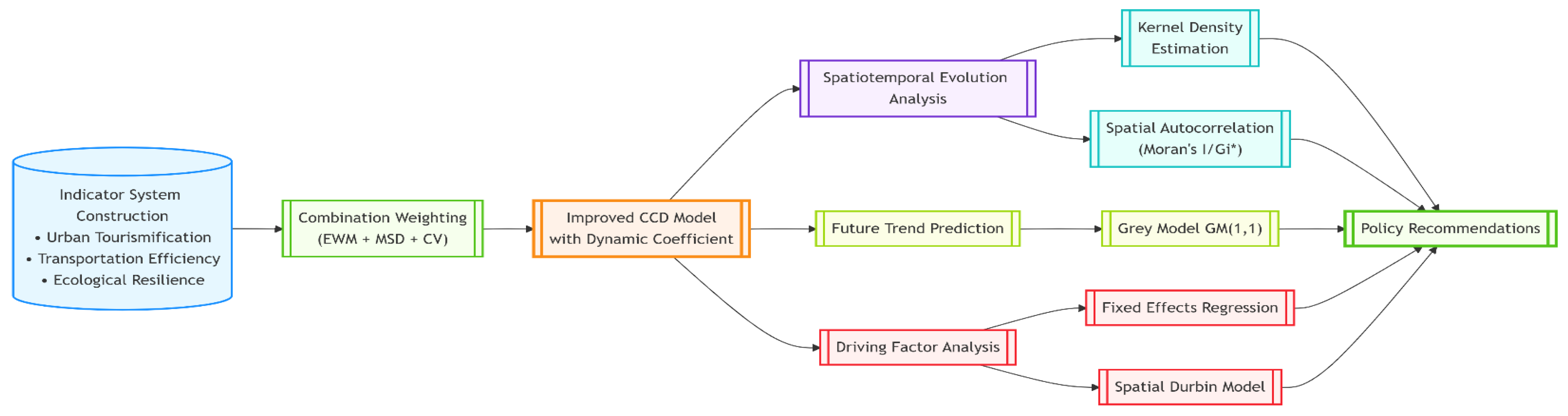
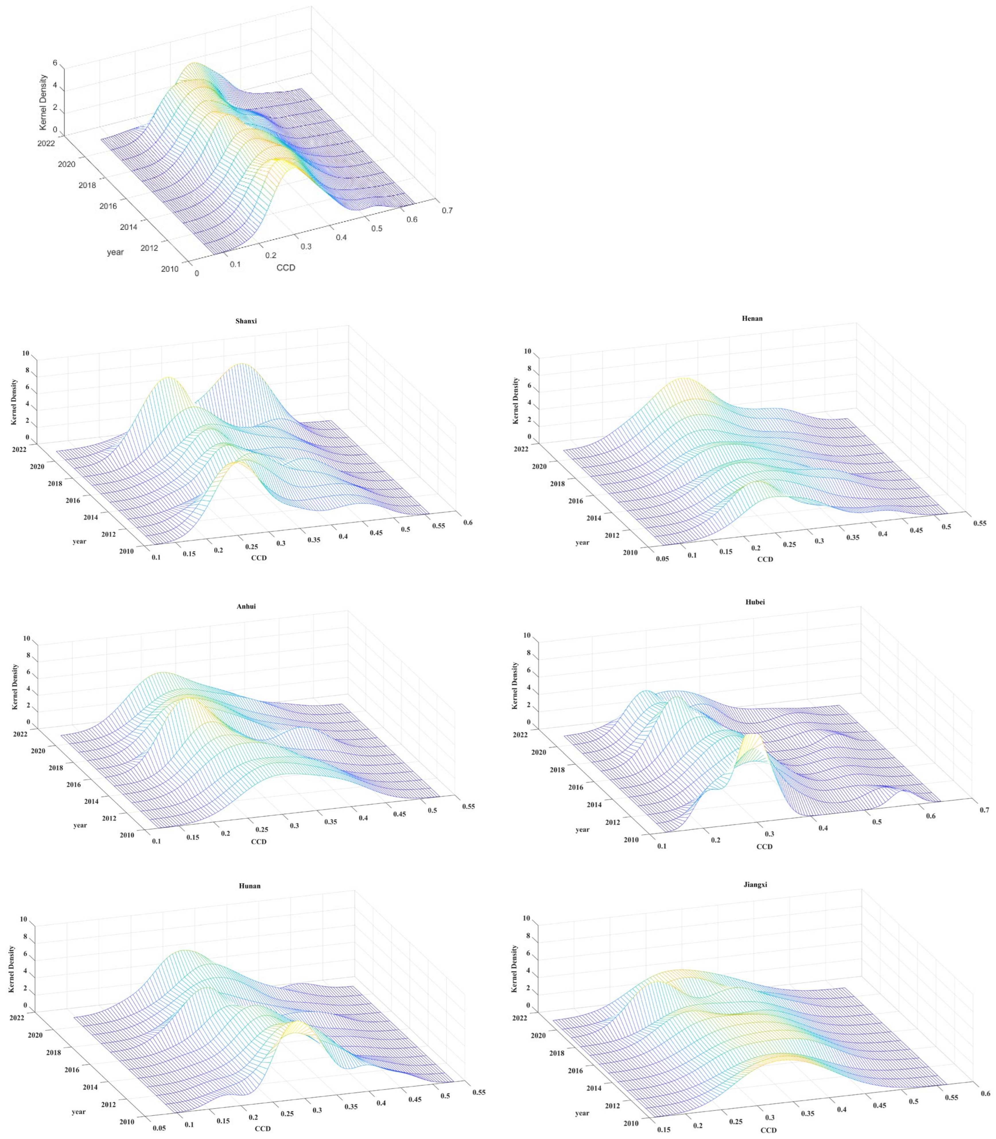
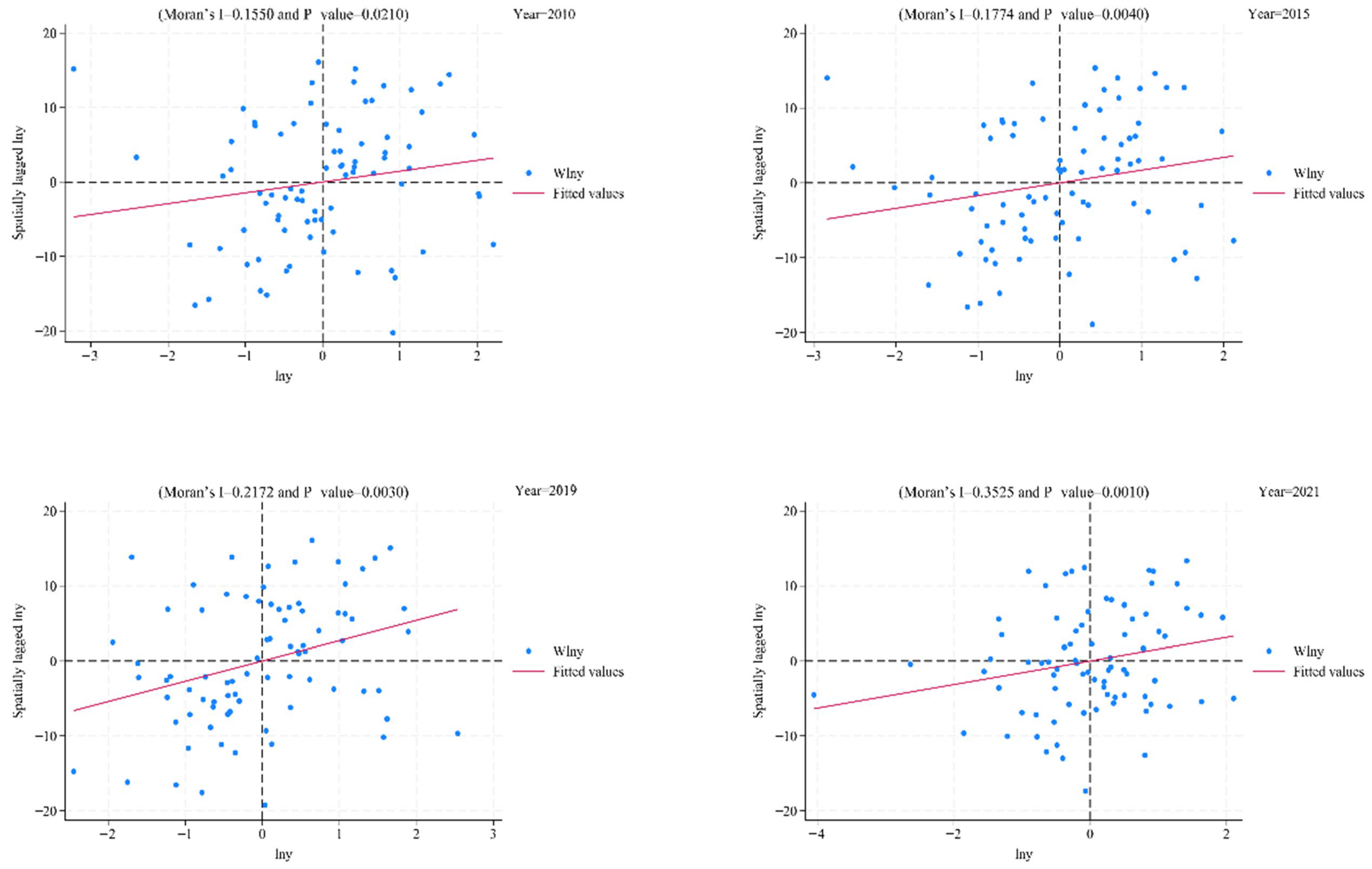
This study utilized an improved CCD model incorporating a time dynamic coefficient for the accurate measurement of the UTTES system. To minimize the influence of subjective bias and extreme values on the dataset, combined weights were calculated using the entropy weight method, mean squared deviation weighting, and coefficient of variation method, resulting in more scientifically robust CCD values. Furthermore, to thoroughly analyze historical development trends and future projections of CCD, kernel density estimation and ArcGIS tools were utilized to explore the overall developmental trajectory and spatiotemporal evolution of UTTES coupling coordination. Additionally, the GM (1,1) method was applied to forecast future CCD trends. Finally, a fixed effects model was employed to analyze the driving factors of UTTES. Following spatial autocorrelation validation, the analysis was extended using a spatial Durbin model to examine the spatial spillover effects of these driving factors. The following key insights were identified.

5.1. Core Patterns of the UTTES System

The spatiotemporal evolution of the UTTES (Urban Tourism and Transportation Economic System) composite level reveals three globally relevant core patterns. First, the coexistence of growth resilience and vulnerability to risks parallels the ‘boom-bust’ cycles observed in Caribbean tourism economies during the COVID-19 pandemic. Second, regional differentiation mirrors the gradient disparities between Barcelona’s urban core and Catalonia’s hinterlands, where tourism revenue concentration exacerbates peripheral marginalization. Third, structural contradictions echo the tension between industrial land use and ecological zoning observed in Brazil’s Amazonian cities.

Growth Resilience vs. Risk Vulnerability: The UTTES in central China exhibited an upward trend (4.27% annual growth) but declined sharply post-2019 due to COVID-19. This highlights the fragility of tourism-dependent economies to exogenous shocks [50], akin to Caribbean Island nations during pandemic lockdowns.

Regional Differentiation: Jiangxi achieved a high growth rate (5.76%), stemming primarily from the digitization of ecological resources, whereas Henan recorded a low average (0.283), reflecting supply-side inefficiencies. Hubei exhibited a pronounced “core-periphery” divide (Wuhan > 0.4 vs. others < 0.4 in UTTES levels), similar to the tourism revenue concentration observed in Barcelona [48].

Structural Contradictions: Cities like Zhengzhou experienced “valley events” (periods of significant decline), indicating that traditional development models heavily reliant on infrastructure investment face dual pressures from ecological capacity limits and rising market demands. These structural contradictions closely mirror the industrial–ecological conflicts documented in Brazil’s Amazonian cities [49].

Practical Relevance to Socioeconomic Well-being: Research findings underscore that balanced UTTES development directly enhances human well-being. For instance,

Cities with high CCD (e.g., Wuhan, Changsha) demonstrated stronger recovery in post-pandemic employment and tourism income, thereby supporting progress towards SDG 8 (decent work) and SDG 11 (sustainable cities).

Lagging transportation efficiency (e.g., in Jiangxi) correlated with reduced accessibility to healthcare and education for rural tourists, exacerbating social inequity. This aligns with studies linking transport poverty to multidimensional deprivation in Global South cities [2].

5.2. Driving Factors and Spatial Spillover Effects

Fixed effects and spatial Durbin models (SDM) were employed in this study to investigate the driving factors of UTTES development and their spatial spillover effects. The results indicate that economic activity levels, social structural transformation, and policy support strength significantly drive the UTTES system. The analysis identified PG, LDF, FC, UL, SSR, TSR, and ER as the key drivers of UTTES coupling coordination. These findings align with the “growth pole” theory, where capital-intensive investments in transportation infrastructure and tourism facilities enhance accessibility and ecological governance through multiplier effects [52,53].

However, SSR exhibits a significant negative impact, revealing a critical contradiction: while industrial agglomeration drives economic growth, it simultaneously exacerbates pollution, encroaches on ecological spaces, and impedes tourism experience quality and ecosystem restoration. This observation supports the Environmental Kuznets Curve (EKC) hypothesis, indicating that central China—as a middle-income region—faces a trade-off between industrialization and sustainable tourismification.

The SDM further highlights asymmetric spatial spillovers. Positive spillovers from PG and LDF suggest economically developed cities (e.g., Wuhan, Zhengzhou) act as growth engines, diffusing capital and green technologies to neighboring areas through industrial linkages and policy imitation. Conversely, negative spillovers from UL, FC, SSR, and TSR indicate a “siphoning effect,” where foreign capital and industrial clusters concentrate in core cities, depleting peripheral resources and widening CCD coordination gaps.

Notably, the SSR-UTTES contradiction is not absolute; it can be mitigated through smart manufacturing, industry–city integration, and ecological compensation strategies to foster composite industrial–tourism growth. This spatial polarization reflects “core-periphery” dynamics in regional economics, underscoring the necessity for cross-administrative governance coordination.

5.3. Policy Implications

Based on the historical–spatiotemporal evolution, projected trends, and identified drivers of the UTTES system, this study proposes policy recommendations across three domains. Institutional–Technological Coordination Mechanism: Post-pandemic governance necessitates a transition from fragmented sectoral management toward a government–industry–academia co-evolution model [65], with emphasis on institutional coordination, technological empowerment, and spatial restructuring. Specific measures include the following: 1. Establishing cross-provincial tourism risk prevention mechanisms for public health emergencies. 2. Piloting blockchain-based big data regulatory systems in central China. 3. Developing cross-regional cultural corridors and tourism enclave economic zones (e.g., in polarized regions like Hubei), supported by fiscal incentives for core-periphery tourism revenue sharing. Differentiated Resilience Strategies for Heterogeneous Regions: Building on spatial Durbin model results, tailored pathways are recommended: 1. Industrial-intensive cities (e.g., Zhengzhou): Analysis suggests prioritizing eco-tourism infrastructure and heritage digitization for surplus fund allocation, strengthening cultural preservation and environmental resilience. 2. Tourism-dependent cities: Seasonal adjustment strategies can be achieved through institutional partnerships (e.g., winter wellness tourism collaborations between destination operators and healthcare providers), mitigating demand volatility and optimizing resource allocation. 3. Transportation hubs: Transit-oriented development principles should integrate low-carbon mobility and the “15-min tourism” framework [66], mandating ≤500 m pedestrian access between 4A-rated attractions and subway hubs with synchronized shuttle services. Digital-Era Tourism Governance System: A tripartite implementation framework is proposed, comprising the following: (1) A spatiotemporal early warning system utilizing machine learning algorithms (e.g., Baidu migration indices, Ctrip booking data) for predictive CCD threshold monitoring. (2) A policy impact simulator employing multi-agent modeling to assess fiscal intervention efficacy. (3) A stakeholder co-creation model leveraging blockchain technology for participatory tourism budgeting and infrastructure financing. The specific implementation pathways are as follows: Green Infrastructure Financing: Introduce public–private partnerships (e.g., EU Connecting Europe Facility model) for rail-electrification in lagging cities (Kaifeng, Anqing) to counter SDM-identified “siphoning effects”. Ecological Compensation: Mandate manufacturing-sector ecological taxes in industrial hubs (e.g., Zhengzhou) to fund urban green corridors (e.g., Wuhan’s “30 km Greenway Initiative”). Global South Adaptations: Scale UTTES via context-sensitive transport solutions: boat transit networks in archipelagic Southeast Asia (Jakarta) and minibus electrification in African cities (Nairobi) to balance cost-emission goals.

5.4. International Applicability of the UTTES Framework

The UTTES framework offers scalable insights beyond China: Latin America: In Medellín, Colombia, cable-car systems enhanced tourism accessibility within mountainous informal settlements yet compromised ecological resilience through induced soil erosion. The UTTES framework provides a mechanism to quantify and optimize such spatial trade-offs via the proposed CCD model. Southeast Asia: Bangkok’s “overtourism” crisis (transport congestion, temple degradation) mirrors Zhengzhou’s pre-2019 peak. Our GM (1,1) projections provide early-warning thresholds for visitor caps. Africa: Rwanda’s Nyungwe National Park exemplifies “eco-driven” coordination high $\left({\mathrm{T}}_{\mathrm{e}\mathrm{c}\mathrm{o}\mathrm{l}\mathrm{o}\mathrm{g}\mathrm{y}}^{\mathrm{*}}\right)$, akin to Huangshan. However, weak spatial spillovers in our SDM suggest cross-border governance (e.g., East African Community) is critical for scaling success. Limitations in data-scarce regions (e.g., Sub-Saharan Africa) can be mitigated by proxy indicators (e.g., mobile data for tourism flows, satellite imagery for green space).

5.5. Limitations

While this study quantifies the Urban Tourismification–Transportation Quality–Ecological Resilience System (UTTES) via an improved coupling coordination degree (CCD) model and analyzes spatiotemporal trends using kernel density estimation and GM (1,1) forecasting, several limitations persist due to the system’s inherent complexity: Temporal Granularity: The reliance on annual data may obscure short-term fluctuations and shocks within the CCD. Uncertainty and Sensitivity in Weighting: The CCD results are acknowledged to be sensitive to the weighting schemes employed. To address this, a Monte Carlo simulation (1000 iterations) was conducted to test the robustness of the combined weighting approach (entropy method + mean squared deviation + coefficient of variation). The simulation demonstrated that CCD values varied within a range of ±0.03 (95% confidence interval), confirming overall stability. However, sensitivity analysis identified transportation efficiency indicators (X₁₂–X₁₉) as exhibiting the highest volatility (±4.7%). This suggests that for cities characterized by underdeveloped transport infrastructure (e.g., Jiangxi), projections would benefit significantly from higher-resolution data to reduce uncertainty. Future research should incorporate stochastic weighting or Bayesian approaches to better capture the inherent dynamics of the system. Indicator Scope: The current urban tourismification metrics lack behavioral dimensions. Future work should integrate sources like mobile GPS data to refine resident mobility measurements. Spatial Mechanism “Black Box”: The drivers underlying observed spatial spillover effects remain inadequately explored. Integrating qualitative methodologies is recommended to elucidate the governance pathways and causal mechanisms involved.

6. Conclusions

This study employed an improved coupling coordination degree (CCD) model, kernel density estimation, GM (1,1) forecasting, fixed effects regression, and spatial Durbin regression models to analyze the spatiotemporal evolution of the Urban Tourism–Transportation–Ecology System (UTTES) across eighty cities in central China. The analysis identified response thresholds and mechanisms of the UTTES to variations in economic activity levels, social structural transformation, and policy support strength.

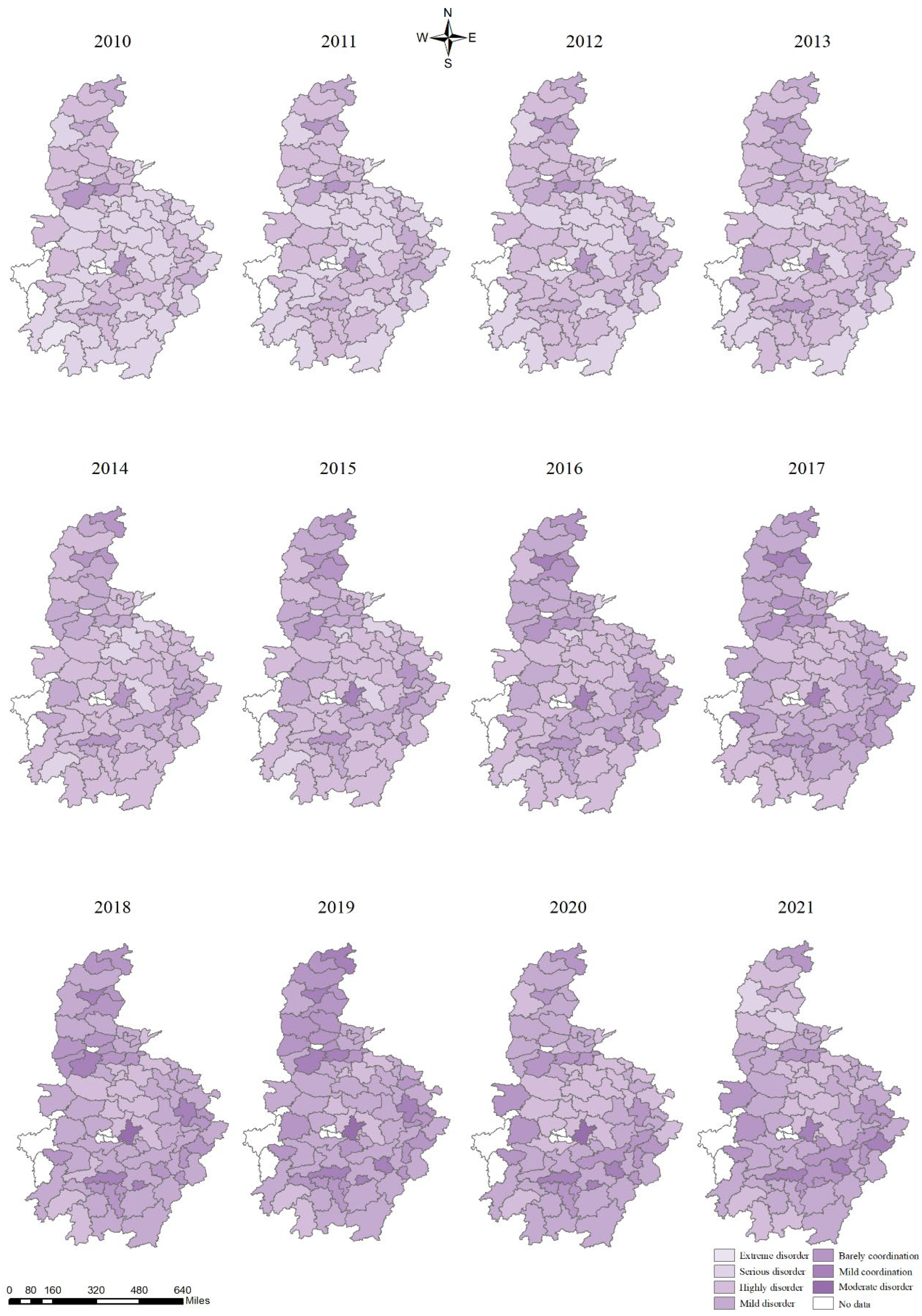
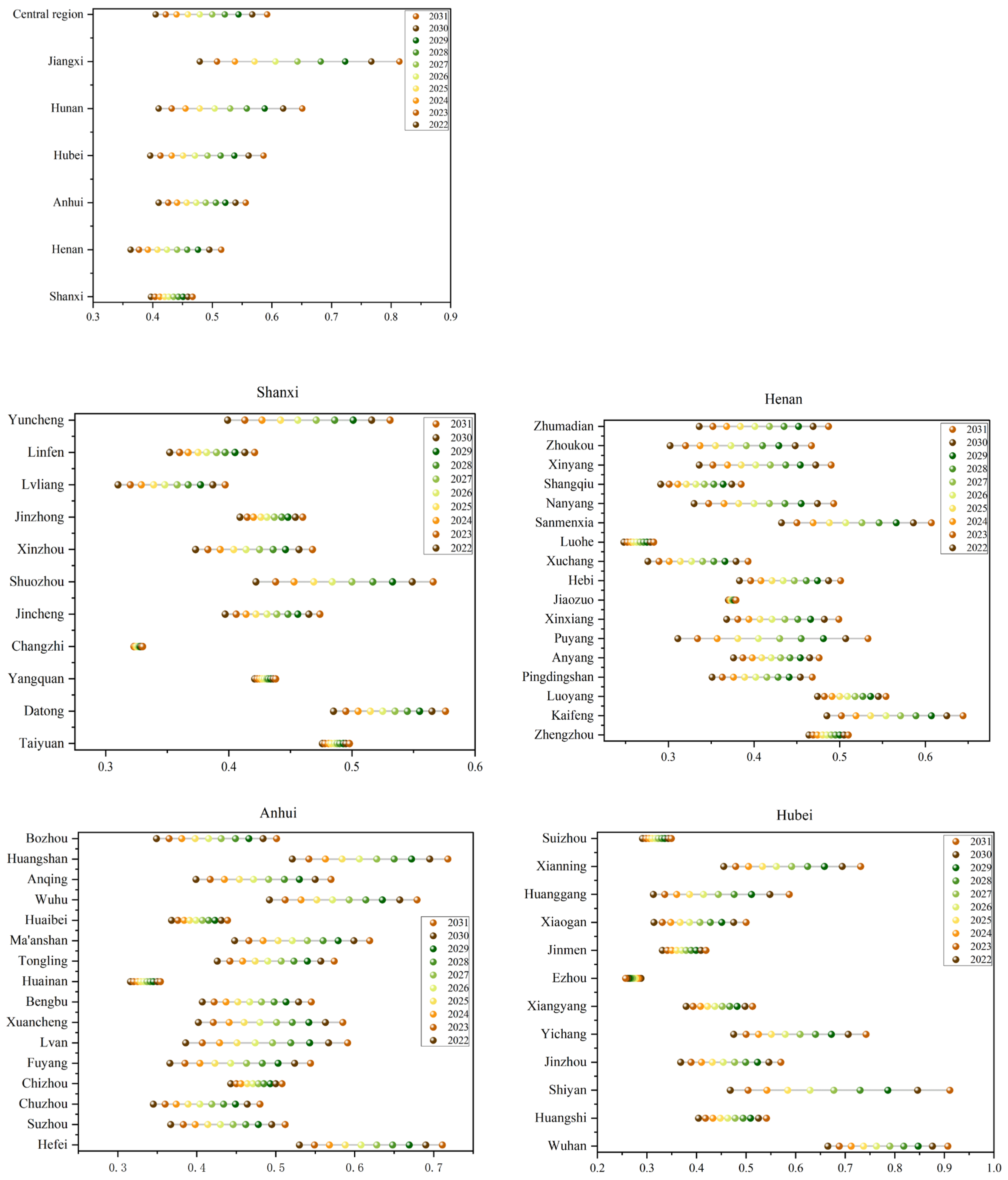
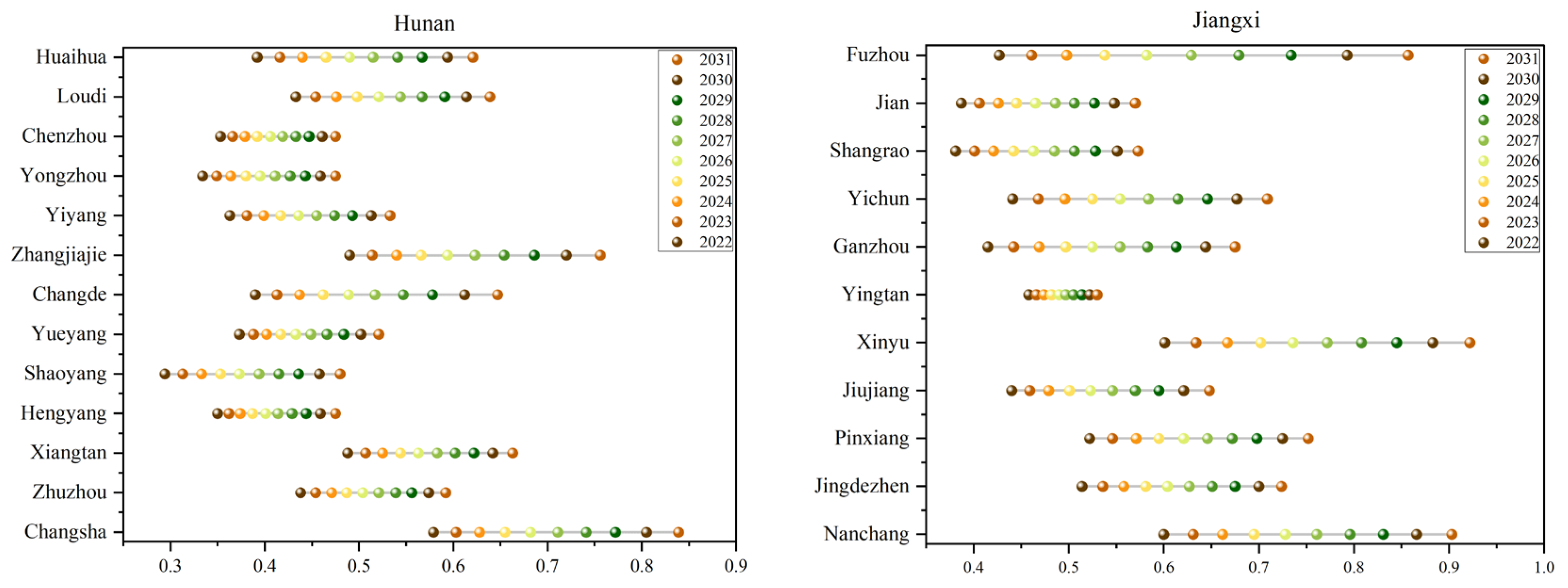
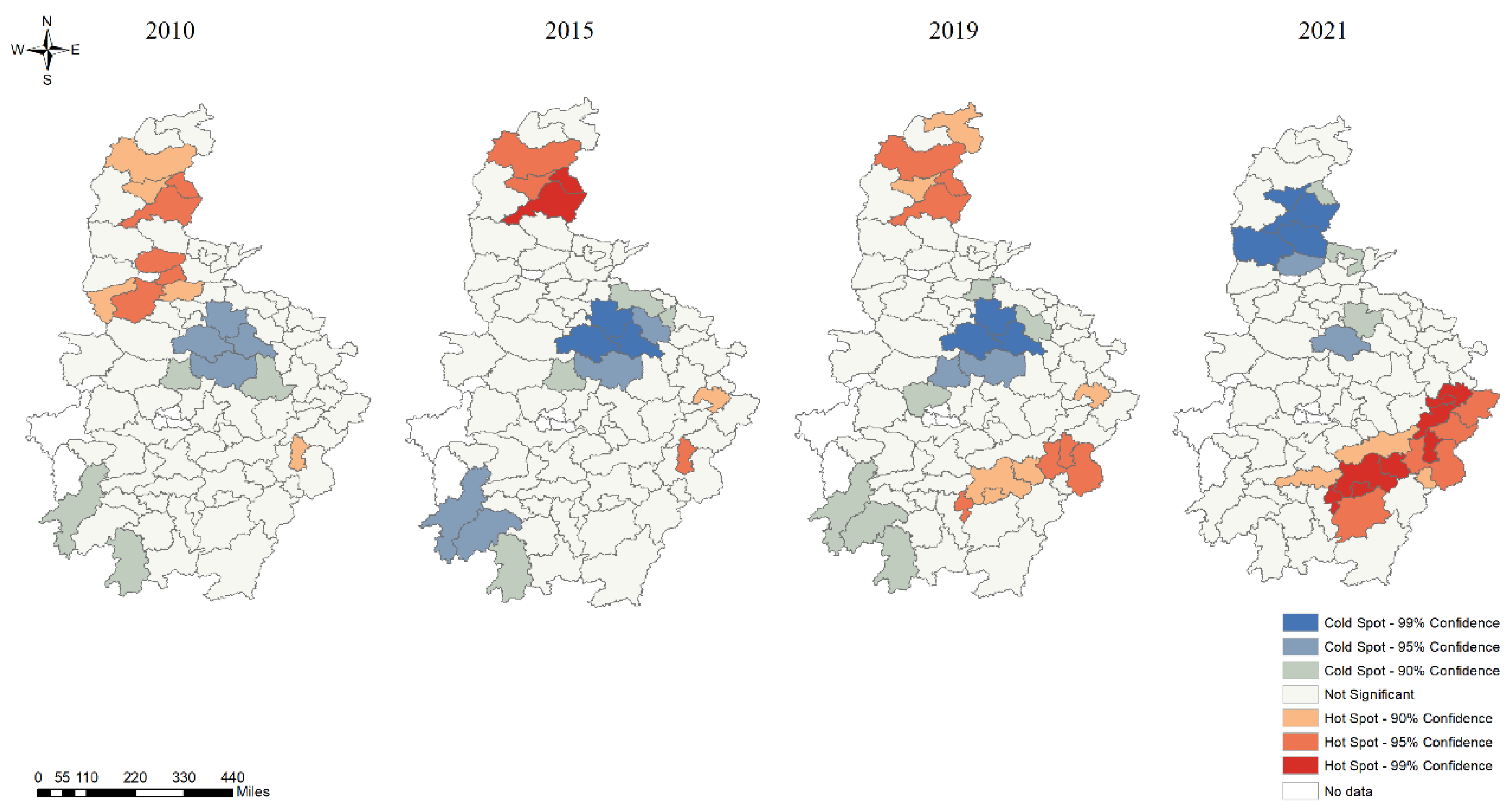
The analysis identified major transportation infrastructure development, ecological tourism transitions, and policy coordination as primary determinants of CCD peak value fluctuations. Subsequent driving factor analysis confirmed these relationships. Spatial diagnostics for the terminal observation year revealed relative equilibrium within the ecological resilience subsystem, with disequilibrium predominantly localized in the tourism–economic and transport–logistical subsystems. Spatial distribution analysis revealed a predominance of tourismification-lagging cities, with most simultaneously exhibiting non-lagged transportation development. Eco-driven development patterns characterized Huangshan, Changsha, and Nanchang, contrasting with Wuhan’s distinct transportation-driven growth paradigm. From 2010 to 2019, the UTTES CCD was classified into seven categories: extreme disorder, serious disorder, highly disordered, mild disorder, barely coordinated, mildly coordinated, and moderately coordinated. Post-2014, the number of cities achieving coordinated development increased. The average CCD value rose from 0.220 in 2010 to 0.349 in 2021, peaking prior to the impact of COVID-19. Shanxi Province recorded the highest average CCD value, followed by Jiangxi, Anhui, Hubei, Hunan, and Henan. Notable disparities in CCD values were observed among cities within Hubei Province. Spatially, the CCD distribution exhibited a “periphery-center” hierarchical structure, with high-value regions concentrated in provincial capitals and tourism cities, while low-value regions were found in eastern Hubei and eastern Henan. Future projections suggest the central region will reach the mild coordination phase by 2031, with Jiangxi Province projected to lead by achieving the good coordination phase in that year. Furthermore, the UTTES operates through a dual-path driving mechanism: economic development and financial growth serve as primary positive drivers while manufacturing intensity and stringent environmental regulations present significant obstacles. The core issue involves spatial spillover effects, whereby core cities exacerbate regional differentiation through processes of technological diffusion and resource siphoning.

Theoretical Contribution: This study makes a significant theoretical contribution by proposing the UTTES framework. This framework transcends fragmented approaches focusing solely on sustainable urban development, tourism-driven gentrification, or ecological urbanism. It explicitly integrates and quantifies the complex, dynamic coupling coordination among three critical urban subsystems: tourism, transportation, and ecology. By employing an improved CCD model incorporating temporal dynamics and robust weighting methods (entropy weight, mean squared deviation, coefficient of variation), the framework provides a novel, holistic lens for assessing urban sustainability. It uniquely captures the tensions and synergies between economic growth imperatives (e.g., tourism revenue, infrastructure investment) and ecological constraints, revealing mechanisms such as the dual-path driving (positive finance/growth versus negative manufacturing/environmental intensity) and spatial spillovers (growth engines versus siphoning effects) that shape regional disparities. This addresses a critical gap in understanding the integrated performance and resilience of cities facing pressures like overtourism and climate change.

International Applicability: The UTTES framework demonstrates the considerable potential for international adaptation. Its core methodology, particularly the improved CCD model and the low-data-demand GM (1,1) forecasting technique, offers a scalable tool for cities across the Global South grappling with similar challenges of balancing tourism growth, transport needs, and ecological preservation. As explored in Section 4.4, the framework provides relevant insights for diverse contexts, such as Medellín (optimizing tourism accessibility versus soil erosion trade-offs), Bangkok (setting visitor cap thresholds using projections to combat overtourism), and Nairobi/Rwanda (implementing context-sensitive transport electrification and evaluating eco-driven coordination). Crucially, the framework can be adapted to data-scarce regions through proxy indicators (e.g., mobile data for tourism flows, satellite imagery for green space). Furthermore, the identified governance challenges, particularly the necessity for cross-administrative coordination highlighted by the spatial spillover effects, resonate strongly with post-industrial cities in advanced economies seeking sustainable transitions and managing regional inequalities.

Practical Implications: The findings yield concrete recommendations for urban planning, sustainable transport, and eco-tourism strategy: Institutional–Technological Coordination: Shift towards government–industry–academia co-evolution models. Establish cross-jurisdictional mechanisms (e.g., tourism risk prevention, blockchain data systems) and develop integrated spatial strategies like cross-regional cultural corridors and tourism enclave economic zones, supported by fiscal incentives for core-periphery revenue sharing. Differentiated Resilience Strategies: Implement tailored approaches: (1) Industrial Hubs (e.g., Zhengzhou): Redirect capital towards eco-tourism and heritage digitization. (2) Tourism-Dependent Cities: Foster seasonal adjustment and wellness tourism partnerships. (3) Transportation Hubs: Integrate low-carbon transport and implement the “15-min tourism city” concept, ensuring scenic spot proximity to transit. Digital-Era Governance: Develop a tripartite system: (1) Spatiotemporal early warning using machine learning (e.g., migration, booking data), (2) Policy impact simulators (multi-agent models), (3) Stakeholder co-creation platforms (e.g., blockchain for participatory budgeting). Green Finance and Compensation: Leverage Public–Private Partnerships (e.g., EU CEF model) for green infrastructure (e.g., rail electrification in lagging cities) and implement ecological taxes in industrial hubs to fund urban green corridors (e.g., greenways). Global South Adaptations: Promote context-sensitive solutions like boat transit networks in archipelagos or minibus electrification in African cities, balancing cost and emissions.

Future studies should integrate climate resilience indicators (e.g., coastal erosion metrics for Small Island Developing States—SIDS) to enhance the framework’s universality. Exploring dynamic feedback mechanisms, such as how eco-tourism revenue can fund transportation upgrades, is also critical. As cities worldwide confront overtourism and the imperative for low-carbon transitions, this study underscores the urgent need to reshape urban development pathways through a lens of fairness and multi-system coordination. The UTTES framework offers a valuable diagnostic and planning tool in this endeavor.

References

1. UNWTO. Tourism and the Sustainable Development Goals—Journey to 2030; UNWTO: Madrid, Spain, 2017; Available online: https://www.e-unwto.org/doi/book/10.18111/9789284419401 (accessed on 1 January 2018).
2. Nag, A.; Sarkar, S. Integrating choice freedom, economic health, and transportation infrastructure to forecast tourism demand: A case study of Bishnupur and its alignment with sustainable development goals. Transp. Policy 2024, 147, 198–214. [Google Scholar] [CrossRef]
3. Zheng, X.; Yang, Z. Coordination or contradiction? The spatiotemporal relationship between ecological environment and tourism development within the tourism ecological security framework in China. Ecol. Indic. 2023, 157, 111247. [Google Scholar] [CrossRef]
4. Klepej, D.; Marot, N. Considering urban tourism in strategic spatial planning. Ann. Tour. Res. Empir. Insights 2024, 5, 100136. [Google Scholar] [CrossRef]
5. Ojeda, A.B.; Kieffer, M. Touristification. Empty concept or element of analysis in tourism geography? Geoforum 2020, 115, 143–145. [Google Scholar] [CrossRef] [PubMed]
6. Pickel-Chevalier, S. Les processus de mise en tourisme d’une ville historique: L’exemple de Rouen. Mondes Du Tour. 2012, 6, 46–60. [Google Scholar] [CrossRef]
7. Zhu, H.; Jia, L. The Form of Urban Tourism Based on the Tourism Urbanization. Econ. Geogr. 2006, 1, 151–155. [Google Scholar] [CrossRef]
8. Jansen-Verbeke, M. Tourismification of historical cities. Ann. Tour. Res. 1998, 25, 739–742. [Google Scholar] [CrossRef]
9. Sequera, J.; Nofre, J. Shaken, not stirred: New debates on touristification and the limits of gentrification. City 2018, 22, 843–855. [Google Scholar] [CrossRef]
10. Kowalczyk-Anioł, J. Rethinking tourism-driven urban transformation and social tourism impact: A scenario from a CEE city. Cities 2023, 134, 104178. [Google Scholar] [CrossRef]
11. Paiva, D. The paradox of atmosphere: Tourism, heritage, and urban liveability. Ann. Tour. Res. 2023, 101, 103600. [Google Scholar] [CrossRef]
12. Khadaroo, J.; Seetanah, B. Transport infrastructure and tourism development. Ann. Tour. Res. 2007, 34, 1021–1032. [Google Scholar] [CrossRef]
13. Nazneen, S.; Xu, H.; Din, N.U. Cross-border infrastructural development and residents’ perceived tourism impacts: A case of China–Pakistan Economic Corridor. Int. J. Tour. Res. 2019, 21, 334–343. [Google Scholar] [CrossRef]
14. Shafique, M.; Iftikhar, G.A. Regional dynamics of China Pakistan economic corridor (CPEC): The case of Gilgit baltistan. J. Hist. Stud. 2017, 3, 15–29. [Google Scholar] [CrossRef]
15. Liu, H.; Zhang, Z.; Cai, X.; Wang, D.; Liu, M. Investigating the driving factors of carbon emissions in China’s transportation industry from a structural adjustment perspective. Atmos. Pollut. Res. 2024, 15, 102224. [Google Scholar] [CrossRef]
16. Walker, B.; Holling, C.S.; Carpenter, S.R.; Kinzig, A. Resilience, adaptability and transformability in social–ecological systems. Ecol. Soc. 2004, 9, 1–9. [Google Scholar] [CrossRef]
17. Croese, S.; Green, C.; Morgan, G. Localizing the sustainable development goals through the lens of urban resilience: Lessons and learnings from 100 resilient cities and cape town. Sustainability 2020, 12, 550. [Google Scholar] [CrossRef]
18. Meerow, S.; Newell, J.P. Urban resilience for whom, what, when, where, and why? Urban Geogr. 2019, 40, 309–329. [Google Scholar] [CrossRef]
19. Holling, C.S. Resilience and stability of ecological systems. Annu. Rev. Ecol. Syst. 1973, 4, 1–23. [Google Scholar] [CrossRef]
20. Kondyli, J. Measurement and evaluation of sustainable development: A composite indicator for the islands of the North Aegean region, Greece. Environ. Impact Assess. Rev. 2010, 30, 347–356. [Google Scholar] [CrossRef]
21. Martin, R.; Sunley, P.; Gardiner, B.; Tyler, P. How regions react to recessions: Resilience and the role of economic structure. Reg. Stud. 2016, 50, 561–585. [Google Scholar] [CrossRef]
22. Li, D.; Yang, W.; Huang, R. The multidimensional differences and driving forces of ecological environment resilience in China. Environ. Impact Assess. Rev. 2023, 98, 106954. [Google Scholar] [CrossRef]
23. Ruiz-Ballesteros, E. Social-ecological resilience and community-based tourism: An approach from Agua Blanca, Ecuador. Tour. Manag. 2011, 32, 655–666. [Google Scholar] [CrossRef]
24. Liu, F.; Zhang, Z.; Shi, L.; Zhao, X.; Xu, J.; Yi, L.; Liu, B.; Wen, Q.; Hu, S.; Wang, X.; et al. Urban expansion in China and its spatial-temporal differences over the past four decades. J. Geogr. Sci. 2016, 26, 1477–1496. [Google Scholar] [CrossRef]
25. Tian, Y.; Zhou, D.; Jiang, G. Conflict or Coordination? Multiscale assessment of the spatio-temporal coupling relationship between urbanization and ecosystem services: The case of the Jingjinji Region, China. Ecol. Indic. 2020, 117, 106543. [Google Scholar] [CrossRef]
26. Cui, X.; Fang, C.; Liu, H.; Liu, X. Assessing sustainability of urbanization by a coordinated development index for an Urbanization-Resources-Environment complex system: A case study of Jing-Jin-Ji region, China. Ecol. Indic. 2019, 96, 383–391. [Google Scholar] [CrossRef]
27. Ma, M.; Tang, J. Interactive coercive relationship and spatio-temporal coupling coordination degree between tourism urbanization and eco-environment: A case study in Western China. Ecol. Indic. 2022, 142, 109149. [Google Scholar] [CrossRef]
28. Han, H.; Guo, L.; Zhang, J.; Zhang, K.; Cui, N. Spatiotemporal analysis of the coordination of economic development, resource utilization, and environmental quality in the Beijing-Tianjin-Hebei urban agglomeration. Ecol. Indic. 2021, 127, 107724. [Google Scholar] [CrossRef]
29. Liu, J.; Tian, Y.; Huang, K.; Yi, T. Spatial-temporal differentiation of the coupling coordinated development of regional energy-economy-ecology system: A case study of the Yangtze River Economic Belt. Ecol. Indic. 2021, 124, 107394. [Google Scholar] [CrossRef]
30. Luo, D.; Liang, L.; Wang, Z.; Chen, L. Zhang Faming. Exploration of coupling effects in the Economy–Society–Environment system in urban areas: Case study of the Yangtze River Delta Urban Agglomeration. Ecol. Indic. 2021, 128, 107858. [Google Scholar] [CrossRef]
31. Zhang, Y.; Zhu, T.; Guo, H.; Yang, X. Analysis of the coupling coordination degree of the Society-Economy-Resource-Environment system in urban areas: Case study of the Jingjinji urban agglomeration, China. Ecol. Indic. 2023, 146, 109851. [Google Scholar] [CrossRef]
32. Cheng, J.; Zhang, X.; Gao, Q. Analysis of the spatio-temporal changes and driving factors of the marine economic–ecological–social coupling coordination: A case study of 11 coastal regions in China. Ecol. Indic. 2023, 153, 110392. [Google Scholar] [CrossRef]
33. Khoshnava, S.M.; Rostami, R.; Zin, R.M.; Štreimikiene, D.; Yousefpour, A.; Mardani, A.; Alrasheedi, M. Contribution of green infrastructure to the implementation of green economy in the context of sustainable development. Sustain. Dev. 2020, 28, 320–342. [Google Scholar] [CrossRef]
34. Qiu, G.; Song, R.; He, S. The aggravation of urban air quality deterioration due to urbanization, transportation, and economic development—Panel models with marginal effect analyses across China. Sci. Total Environ. 2019, 651, 1114–1125. [Google Scholar] [CrossRef]
35. Adams, S.; Boateng, E.; Acheampong, A.O. Transport energy consumption and environmental quality: Does urbanization matter? Sci. Total Environ. 2020, 744, 140617. [Google Scholar] [CrossRef]
36. Zhu, Z.; Lu, C. Life cycle assessment of shared electric bicycle on greenhouse gas emissions in China. Sci. Total Environ. 2023, 860, 160546. [Google Scholar] [CrossRef]
37. Qiu, Y.M. Study on sustainable development pattern of ecotourism in less-development areas. Econ. Geogr. 2010, 30, 334–338. [Google Scholar] [CrossRef]
38. Pettas, D.; AvdiKos, V.; IlIopoulos, E.; Karavasili, I. “Insurrection is not a spectacle”: Experiencing and contesting touristification in Exarcheia, Athens. Urban Geogr. 2022, 43, 984–1006. [Google Scholar] [CrossRef]
39. Han, C.; Liu, X.; Shen, X.; Zhang, L.; Feng, N. Evaluating the spatial deprivation of public transportation resources in areas of rapid urbanization: Accessibility and social equity. Discret. Dyn. Nat. Soc. 2019, 2019, 6890362. [Google Scholar] [CrossRef]
40. Chen, Z.; Antunes, J.; Wanke, P.; Zhou, M. Sustainability drivers in road transportation system: Evidence from China. Sci. Total Environ. 2021, 798, 149259. [Google Scholar] [CrossRef]
41. Wang, F.; Li, J.; Yu, F.; He, H.; Zhen, F. Space, function, and vitality in historic areas: The tourismification process and spatial order of Shichahai in Beijing. Int. J. Tour. Res. 2018, 20, 335–344. [Google Scholar] [CrossRef]
42. Kruszyna, M.; Śleszyński, P.; Rychlewski, J. Dependencies between demographic urbanization and the agglomeration road traffic volumes: Evidence from Poland. Land 2021, 10, 47. [Google Scholar] [CrossRef]
43. Yao, J.; Xu, P.; Huang, Z. Impact of urbanization on ecological efficiency in China: An empirical analysis based on provincial panel data. Ecol. Indic. 2021, 129, 107827. [Google Scholar] [CrossRef]
44. Moll, R.J.; Cepek, J.D.; Lorch, P.D.; Dennis, P.M.; Tans, E.; Robison, T.; Millspaugh, J.J.; Montgomery, R.A. What does urbanization actually mean? A framework for urban metrics in wildlife research. J. Appl. Ecol. 2019, 56, 1289–1300. [Google Scholar] [CrossRef]
45. Zhao, X.; Sun, B. The influence of Chinese environmental regulation on corporation innovation and competitiveness. J. Clean. Prod. 2016, 112, 1528–1536. [Google Scholar] [CrossRef]
46. Li, Y.; Li, Y.; Zhou, Y.; Shi, Y.; Zhu, X. Coupling coordination and spatiotemporal dynamic evolution between social economy and water environmental quality—A case study from Nansi Lake catchment, China. Ecol. Indic. 2022, 135, 108543. [Google Scholar] [CrossRef]
47. Sheller, M. Reconstructing tourism in the Caribbean: Connecting pandemic recovery, climate resilience and sustainable tourism through mobility justice. J. Sustain. Tour. 2021, 29, 1436–1449. [Google Scholar] [CrossRef]
48. Romão, J.; Guerreiro, J.; Rodrigues, P.M. Tourism growth and regional resilience: The ‘beach disease’ and the consequences of the global crisis of 2007. Tour. Econ. 2016, 22, 699–714. [Google Scholar] [CrossRef]
49. Gomes Oliveira, A.; Souza Machado, R.A.; Lois González, R.C. Environmental Zoning in a Context of Strong Pressure from Productivist Agriculture in Brazil’s Northeast: The Case of the Ipojuca River, Pernambuco, Brazil. Land 2022, 11, 611. [Google Scholar] [CrossRef]
50. Wu, T.P.; Wu, H.C.; Liu, S.B.; Wu, C.F. Causality between global economic policy uncertainty and tourism in fragile five countries: A three-dimensional wavelet approach. Tour. Recreat. Res. 2021, 47, 608–622. [Google Scholar] [CrossRef]
51. Almeida-Santana, A.; David-Negre, T.; Moreno-Gil, S. New digital tourism ecosystem: Understanding the relationship between information sources and sharing economy platforms. Int. J. Tour. Cities 2020, 6, 335–345. [Google Scholar] [CrossRef]
52. Zhang, Z.; Li, L.; Guo, Q. The Interactive Relationships between the Tourism-Transportation-Ecological Environment System of Provinces along the ‘Silk Road Economic Belt’ in China. Sustainability 2022, 14, 3050. [Google Scholar] [CrossRef]
53. Feng, X.B. Coupling and coordinated development of traffic accessibility and regional tourism economy. Res. Transp. Bus. Manag. 2023, 49, 101010. [Google Scholar] [CrossRef]
54. Mastercard. Global Destination Cities Index 2019. Available online: https://www.mastercard.com/news/media/wexffu4b/gdci-global-report-final-1.pdf (accessed on 4 September 2019).
55. Wang, C.W.; Guo, M.C. Study on touristzation level measurement based on tourism regional system and GIS. China Popul. Resour. Environ. 2018, 28 (Suppl. 2), 76–81. [Google Scholar]
56. Zhang, Y.; Sun, M.; Yang, R.; Li, X.; Zhang, L.; Li, M. Decoupling water environment pressures from economic growth in the Yangtze River Economic Belt, China. Ecological Indicators. 2021, 122, 107314. [Google Scholar] [CrossRef]
57. Gunderson, L.H.; Holling, C.S. Panarchy: Understanding Transformations in Human and Natural Systems; Island Press: Washington, DC, USA, 2002. [Google Scholar]
58. United Nations Environment Programme (UNEP). Global Environment Outlook 3: Past, Present, and Future Perspectives; United Nations Environment Programme: Nairobi, Kenya, 2002; Available online: https://www.unep.org/resources/global-environment-outlook-3 (accessed on 10 November 2002).
59. Berkes, F.; Colding, J.; Folke, C. Navigating Social-Ecological Systems: Building Resilience for Complexity and Change; Cambridge University Press: Cambridge, UK, 2003. [Google Scholar]
60. Holling, C.S. Adaptive Environmental Assessment and Management; John Wiley & Sons: New York, NY, USA, 1978. [Google Scholar]
61. Scheffer, M.; Carpenter, S.R.; Foley, J.A.; Folke, C.; Walker, B. Catastrophic shifts in ecosystems. Nature 2001, 413, 591–596. [Google Scholar] [CrossRef] [PubMed]
62. Ni, R.; Wang, F.; Yu, J. Spatiotemporal changes in sustainable development and its driving force in the Yangtze River Delta region, China. J. Clean. Prod. 2022, 379, 134751. [Google Scholar] [CrossRef]
63. Jiang, X.; Lu, X.; Liu, Q.; Chang, C.; Qu, L. The effects of land transfer marketization on the urban land use efficiency: An empirical study based on 285 cities in China. Ecol. Indic. 2021, 132, 108296. [Google Scholar] [CrossRef]
64. Li, J.; Lin, B. Does energy and CO2 emissions performance of China benefit from regional integration? Energy Policy 2017, 101, 366–378. [Google Scholar] [CrossRef] [PubMed]
65. Etzkowitz, H.; Leydesdorff, L. The dynamics of innovation: From National Systems and “Mode 2” to a Triple Helix of university–industry–government relations. Res. Policy 2000, 29, 109–123. [Google Scholar] [CrossRef]
66. Moreno, C.; Allam, Z.; Chabaud, D.; Gall, C.; Pratlong, F. Introducing the “15-Minute City”: Sustainability, resilience and place identity in future post-pandemic cities. Smart Cities 2021, 4, 93–111. [Google Scholar] [CrossRef]
Figure 1. Mechanism for coupling coordination of urban tourism, transport, and the environment.
Land 14 01263 g001
Figure 2. Urban Tourismification–Transportation Quality–Ecological Resilience System.
Land 14 01263 g002
Figure 3. Location of the study area.
Land 14 01263 g003
Figure 4. Methodological framework for UTTES analysis.
Land 14 01263 g004
Figure 5. Kernel density estimation plot.
Land 14 01263 g005
Figure 6. CCD levels of the six central provinces.
Land 14 01263 g006
Figure 7. Spatial distribution of CCD types.
Land 14 01263 g007
Figure 8. Distribution of predicted CCD.
Land 14 01263 g008aLand 14 01263 g008b
Figure 9. Global spatial autocorrelation of CCD.
Land 14 01263 g009
Figure 10. Local spatial autocorrelation of CCD.
Land 14 01263 g010