Spatial–Temporal Characteristics and Influencing Factors of Carbon Emission Performance: A Comparative Analysis Between Provincial and Prefectural Levels from Global and Local Perspectives

Abstract

To support China’s “3060” dual carbon targets, this study quantitatively evaluates the spatial–temporal characteristics and influencing factors of carbon emission performance (CEP) across administrative levels. While prior research has examined CEP patterns, a systematic comparison of factor contributions at different levels—particularly from global and local perspectives—is lacking. This study addresses this gap by analyzing CEP in 31 provinces and 333 prefecture-level cities (2003–2020) using a coupling coordination degree model to measure CEP, spatial autocorrelation indices (Moran’s I) to assess global/local dependence, static/dynamic Spatial Durbin model (SDM/DSDM) with two-way fixed effects to compare global impacts, and geographically and temporally weighted regression (GTWR) to quantify spatiotemporal heterogeneity. The results show the following: (1) CEP showed consistent growth at both levels with positive spatial autocorrelation, revealing significantly richer clustering patterns at the prefectural rather than provincial level. (2) From a global perspective, influencing factors’ contributions to CEP vary significantly between levels. Provincially, dominant factors rank as time-lagged CEP(CEP_lag)> proportion of built-up land(P_built) > spatial lag of CEP(W×CEP) > fractional vegetation coverage (lnFVC); while prefecturally, CEP_lag > spatial error coefficient(rho) > W×CEP > P_built, with the proportion of secondary industry in GDP (GDP2)/proportion of tertiary industry in GDP (GDP3) gaining greater significance. (3) Local regression results reveal significant spatiotemporal heterogeneity in CEP influencing factors. lnFVC and W×CEP show the most distinct differences between levels, while land-use factors like P_built and nighttime light index (NTL) exhibit unstable spatiotemporal effects. The study underscores the need for scale-specific policies addressing spatial spillovers and local heterogeneity, providing actionable insights for China’s carbon mitigation strategies.

1. Introduction

With the rapid advancement of global industrialization and urbanization, the combustion of fossil fuels has surged, leading to a significant increase in CO₂ emissions [1]. This trend has profound implications for global climate change and sustainable development, making CO₂ emission reduction a critical global priority [2,3]. As the largest developing country in the 21st century, China faces substantial challenges in mitigating its CO₂ emissions [4]. In response, the Chinese government has integrated CO₂ emission reduction targets into the national “14th Five-Year Plan” and the long-term goals for 2035, underscoring its commitment to addressing this issue [5,6,7]. Achieving these targets requires not only controlling the scale and intensity of carbon emissions but also emphasizing the quality of development and improvements in living standards [8]. Carbon emission performance (CEP), which reflects the input–output relationship of economic activities, is closely tied to the realization of carbon reduction targets and low-carbon economic development [9,10]. Enhancing CEP is thus pivotal to achieving carbon emission reduction goals [11]. Identifying the key factors influencing CEP holds significant practical importance for advancing China’s green and low-carbon transition [12,13,14].

CEP represents the outcome of changes in the relationship between factor inputs and final outputs in socio-economic development and serves as a critical indicator for evaluating green and low-carbon economic development [10]. Current methodologies for measuring CEP can be categorized into single-factor and total-factor approaches [15]. Single-factor CEP measures performance using unit carbon emissions associated with various economic and social phenomena, such as total carbon emissions [16], carbon emissions per unit of energy consumption, carbon productivity (GDP per unit of CO₂ emissions) [17], carbon emission intensity (CO₂ emissions per unit of GDP), and per capita carbon emissions (CO₂ emissions per capita) [18]. For instance, Zheng et al. [19] employed carbon emission intensity as a proxy for CEP to assess the impact of China’s emission trading scheme pilot policy using a Difference-in-Differences (DID) model. In contrast, total-factor CEP incorporates both expected and unexpected outputs into the evaluation system, making it a more comprehensive and widely used approach [20]. Common models for total-factor CEP include the slack-based measure (SBM) model [21], data envelopment analysis (DEA) [2], stochastic frontier analysis (SFA), super-efficiency SBM model [22], Super-EBM model [14,23], Malmquist index decomposition [24], non-radial distance functions, and the Malmquist–Luenberger index model [25]. Single-factor CEP is straightforward to calculate [26], while total-factor CEP considers the relative relationship between actual and expected outputs under specific economic and technological conditions [20,27]. However, both single-factor and total-factor approaches, grounded in neoclassical economics, fail to capture societal non-market welfare outputs. From an ecological economics perspective, the comprehensive CEP assessment framework integrates three dimensions: economic output, population carrying capacity, and living standard [28]. The coupling coordination degree model enables calculation of both individual efficiencies and their systemic coordination [23,29], providing a balanced measure of regional low-carbon performance and supporting differentiated responsibility allocation.

Building on the measurement of CEP, previous studies have extensively explored its spatial–temporal evolution patterns [23] using methods such as regional numerical differences, Theil index, exploratory spatial analysis (ESTDA) [30], kernel density estimation, and the Gini coefficient to study spatial distribution heterogeneity [31,32], spatial autocorrelation (global and local Moran’s I index) [32,33], Markov chain transition matrices [34], and social network analysis [22]. Recently, scholars have increasingly focused on identifying the influencing factors of CEP to promote carbon emission reduction [27,35]. Socio-economic and land-use-related factors affecting CEP are complex and diverse [12,23,32]. Previous studies have qualitatively and quantitatively analyzed factors such as urbanization level, economic development, industrial structure, green finance, energy consumption, technological innovation, energy intensity, and population density [36,37]. Land-use management, as a coupling system linking socio-economic activities and natural ecosystems, plays a critical role in CEP [16]. With the availability of multi-source data, scholars have begun incorporating land-use-related factors, such as land-use intensity, nighttime light index, and urban landscape pattern [38] into CEP analyses [16,17]. Methods for identifying influencing factors include decomposition techniques (e.g., factor decomposition, input–output models, and LMDI) [39,40], coefficient methods (e.g., correlation analysis and grey correlation analysis), equation methods (e.g., panel quantile regression [12], threshold effect models [37], and spatial econometric models [41,42,43]), and causality methods (e.g., Granger causality tests). Geographic weighted regression (GWR) models [44], Geographical detector (GD) [45], and difference-in-differences (DID) models [11,46] have also been widely used. For instance, Liu et al. [47] explored the spatial characteristics of city-level CO₂ emissions and their influencing factors from global and local perspectives using spatial autocorrelation analysis and regression models. While global regression models like the Spatial Durbin model [35,48] are commonly used, dynamic Spatial Durbin models (DSDMs) [49] and local regression models like geographically and temporally weighted regression (GTWR) [50,51] are underutilized. The DSDM serves as a global analytical approach capable of capturing spatiotemporal dependencies and dynamic spillover effects, while GTWR provides an advanced local perspective to address spatial heterogeneity and temporal non-stationarity [52,53]. Their integrated application establishes a robust framework for examining the influencing factors of CEP, as they collectively account for both global interactions and localized dynamics. Notably, few studies have systematically combined the DSDM and GTWR to analyze CEP impacts [47], underscoring the methodological novelty of this approach.

Despite extensive research investigating the measurement, spatiotemporal evolution, and influencing factors of CEP [36], significant variations exist in analytical scales across studies, encompassing national, provincial [27,44], prefecture-level [54,55], economic zones [56,57], and county-level [58,59] analyses. For instance, one study [23] analyzed the evolutionary characteristics and driving factors of urban CEP across 191 prefecture-level cities (1997–2017). Another study, using provincial panel data (30 regions, 1997–2017), integrated environmental production technology and stochastic frontier models to assess the spatiotemporal dynamics of total-factor CEP and evaluate policy effectiveness [27]. These works provide critical insights into the complexity of regional inequalities in socioeconomic development. However, since socioeconomic factors—including CEP and its drivers—exhibit significant scale dependence, findings at one spatial scale cannot be directly extrapolated to another. Growing scholarly consensus emphasizes that comparative analyses of CEP characteristics and determinants across scales are essential for a deeper understanding of geographic phenomena. Prior studies have systematically neglected cross-administrative CEP comparisons. Beyond [60]’s provincial–prefectural CO₂ emission analysis, no research has integrated the coupling coordination degree model with spatial econometric techniques (the DSDM and GTWR) for multi-scale CEP assessment—a critical gap in understanding global and local CEP dynamics across administrative levels.

To address these research gaps, this study conducts a comparative analysis of CEP characteristics and their driving factors across both provincial and prefectural administrative levels (31 provinces and 333 prefecture-level cities from 2003 to 2020) in China from global and local perspectives. The analysis proceeds in four stages: (1) The coupling coordination degree model was used to calculate CEP. (2) Global and local spatial autocorrelation analyses were conducted to examine spatial spillover effects. (3) Both static and dynamic Spatial Durbin models (SDMs/DSDMs) with two-way fixed effects were estimated to compare influencing factors of CEP at provincial and prefectural levels from a global perspective. (4) The GTWR model was used to analyze the spatial heterogeneity of influencing factors from a local perspective. The findings aim to reveal the spatial scale sensitivity and temporal–spatial hierarchy of CEP influencing factors, providing a scientific basis for regional carbon performance policies.

2. Materials and Methods

2.1. Research Methodology

2.1.1. CEP Measurement

Coordinated development in the context of carbon emissions does not focus solely on optimizing individual elements within the complex system but emphasizes the harmony among multiple elements and the overall optimization of system efficiency. Therefore, this study draws on the coordination model to construct a coordination function for CEP, reflecting the balance among the economic output capacity per unit carbon emissions, the population support capacity per unit of carbon emissions, and the welfare improvement capacity per unit of carbon emissions goals. Three sub-indicators are used to measure CEP: (1) GDP output per unit carbon emission (GDP/CO₂): reflects the economic output capacity per unit carbon emissions. (2) Population carrying capacity per unit carbon emission (Pop/CO₂): reflects the population support capacity per unit of carbon emissions. (3) Per capita disposable income per unit carbon emission (Welfare/CO₂): reflects the welfare improvement capacity per unit of carbon emissions.

The construction of the comprehensive CEP index involves the following steps: (1) Normalization: the three sub-indicators are normalized using the maximum value method to eliminate dimensional differences. (2) Coordination degree calculation: the coordination degree among the three sub-indicators is calculated using a revised coupling coordination degree function. (3) Comprehensive index synthesis: the comprehensive CEP index is derived by integrating the coordination degree and the values of the three sub-indicators.

The revised coupling coordination degree model is based on the work of [61]. The formulas are as follows:

$$C=\sqrt{\left[1-{\displaystyle \frac{\sqrt{\left(U_3-U_1\right)2}+\sqrt{\left(U_2-U_1\right)2}+\sqrt{\left(U_3-U_2\right)2}}{3}}\right]\times \sqrt{{\displaystyle \frac{U_1}{U_3}}\times {\displaystyle \frac{U_2}{U_3}}}}$$

(1)

$$T={\displaystyle \frac{U_1+U_2+U_3}{3}}$$

(2)

$$CEP=\sqrt{C\times T}$$

(3)

where $C$ represents the coordination degree among the three sub-indicators. A higher value indicates better coordination. $T$ is the weighted average of the three sub-indicators, reflecting carbon emission performance without considering coordination. $CEP$ is the comprehensive CEP index. $U_1$, $U_2$, $U_3$ are the three sub-indicators (GDP output per unit carbon emission, population carrying capacity per unit carbon emission, and per capita disposable income per unit carbon emission), assuming max $U_1$, $U_2$, $U_3$ is $U_3$.

2.1.2. Spatial Autocorrelation Model

The spatial autocorrelation model is used to analyze the spatial aggregation characteristics of CEP, examining whether adjacent observations exhibit spatial interaction and interdependence. This study employs both global and local spatial autocorrelation analyses.

Global Spatial Autocorrelation (Moran’s $I$ Index):

$$I={\displaystyle \frac{{\displaystyle {\sum }_{\mathrm{i}=1}^n{\displaystyle {\sum }_{j\ne i}^n{W}_{ij}\left(x_i-\overline{x}\right)\left(y_i-\overline{y}\right)}}}{{\displaystyle {\sum }_{\mathrm{i}=1}^n{\left(x_i-\overline{x}\right)}^2{\displaystyle {\sum }_{j=1}^n{\left(y_i-\overline{y}\right)}^2}}}}$$

(4)

Local Spatial Autocorrelation (Local Moran’s I Index):

$$I_i={\displaystyle \frac{n\left(x_i-\overline{x}\right)\left(y_i-\overline{y}\right){\displaystyle {\sum }_{\mathrm{j}=1}^n{W}_{ij}\left(x_j-\overline{x}\right)\left(y_j-\overline{y}\right)}}{{\displaystyle {\sum }_{j=1}^n{\left(x_j-\overline{x}\right)}^2{\displaystyle {\sum }_{j=1}^n{\left(y_j-\overline{y}\right)}^2}}}}$$

(5)

where $x_i$, $y_i$ represent the CEP values of spatial unit i and spatial unit j, respectively, and $\overline{x}$, $\overline{y}$ respectively represent the mean CEP value; n is the total number of spatial units; and $W_{ij}$ is a spatial weight matrix (Queen’s contiguity matrix is used in this study).

Based on the Local Moran’s I index, CEP is classified into four spatial clusters (LISA clusters): High–High (H–H): High CEP surrounded by high CEP. Low–Low (L–L): Low CEP surrounded by low CEP. Low–High (L–H): Low CEP surrounded by high CEP. High–Low (H–L): High CEP surrounded by low CEP.

2.1.3. Static Spatial Durbin Model (SDM) and Dynamic Spatial Durbin Model (DSDM)

Unlike the Ordinary Least Squares (OLS) model, spatial econometric models offer the distinct advantage of effectively accounting for spatial dependence [17]. Based on the type of spatial interaction, spatial econometric models can be categorized into three primary types: the Spatial Error Model (SEM), the Spatial Lag Model (SLM), and the Spatial Durbin Model (SDM) [62,63]. Compared to the static Spatial Durbin Model, the Dynamic Spatial Durbin Model (DSDM) further addresses endogeneity issues, thereby significantly enhancing the model’s applicability and robustness [64].

In theory, CEP should respond instantaneously to its influencing factors. However, in practice, CEP evolution exhibits strong path dependence, where current changes are constrained by prior conditions, leading to a pronounced time lag effect. This hysteresis underscores the importance of studying temporal delays in CEP dynamics. Furthermore, for enhanced analytical tractability, excluding spatially lagged independent variables achieves model simplification while preserving the model’s fundamental ability to identify key influence factors of CEP.

To comprehensively analyze the temporal and spatial dynamics influencing CEP, this study employs two models: the static Spatial Durbin Model and DSDM. The formulations of these models are as follows:

Static Spatial Durbin Model (SDM):

$$CE{P}_{it}=\rho W\times CE{P}_{it}+{\beta }_i{X}_{it}+{\lambda }_i+o_t+{\epsilon }_{it}$$

(6)

Dynamic Spatial Durbin Model (DSDM):

$$CE{P}_{it}=\alpha CE{P}_{it-1}+\rho W\times CE{P}_{it}+{\beta }_i{X}_{it}+{\lambda }_i+o_t+{\epsilon }_{it}$$

(7)

where $CE{P}_{it}$ is the logarithmic value of CEP for spatial unit i in year t; i denotes a spatial unit; t represents the year; $\alpha$ is the time lag coefficient, measuring the intensity of the time lag effect, indicating the influence of CEP in the previous year on the current CEP; $CE{P}_{it-1}$ is the time lag term; $\rho$ is the coefficient of the spatial lag term of the explained variable; $W$ is the spatial weight matrix; $W\times CE{P}_{it}$ represents the spatial lag term, capturing the influence of neighboring locations; ${\beta }_i$ is the coefficient vector of independent variables; $X_{it}$ is a feature vector composed of influencing factors; ${\lambda }_i$ indicates the individual fixed effect; $o_t$ denotes the time fixed effect; and ${\epsilon }_{it}$ is the residual term, which includes the error term of spatial autocorrelation and the random error term of independent and identical distribution.

2.1.4. Spatiotemporal Geographically Weighted Regression (GTWR)

The GTWR model extends the traditional GWR framework by incorporating a time dimension parameter, enabling it to capture both temporal non-stationarity and spatial heterogeneity in the data [65]. This enhancement allows the GTWR model to effectively reduce model errors and parameter estimation errors, providing more robust and accurate results. Like the DSDM, the GTWR model can also incorporate time lag terms and spatial lag terms to account for temporal and spatial dependencies in the data. This makes the GTWR model a powerful tool for analyzing complex spatiotemporal phenomena, such as CEP.

The formulation of the GTWR model with time lag and spatial lag terms can be expressed as follows:

$$CE{P}_{it}={\beta }_0\left({\mu }_i,v_i,t_i\right)+\alpha \left({\mu }_i,v_i,t_i\right)CE{P}_{it-1}+\rho \left({\mu }_i,v_i,t_i\right)W\times CE{P}_{it}+\beta \left({\mu }_i,v_i,t_i\right)X_{it}+{\mu }_{it}$$

(8)

where ${\beta }_0\left({\mu }_i,v_i,t_i\right)$ is the intercept term, varying with spatial coordinates $\left({\mu }_i,v_i\right)$ and time $t_i$; $\alpha \left({\mu }_i,v_i,t_i\right)$ is the time lag coefficient, which measures the influence of the dependent variable at the previous time period $CE{P}_{it-1}$ on the current value; $\rho \left({\mu }_i,v_i,t_i\right)$ is the spatial lag coefficient; and $\beta \left({\mu }_i,v_i,t_i\right)$ denotes the local regression coefficient for the independent variable, varying with spatial coordinates and time. ${\mu }_{it}$ is the error term at location i and time $t$.

In this study, the GTWR model employs the Gaussian function to construct the spatiotemporal weight matrix, utilizing its smooth decay property to capture spatial dependencies and incorporating a time dimension parameter to reflect spatiotemporal heterogeneity.

2.2. Variable Definition

Explained variable: Carbon emission performance (CEP).

Explanatory variables: Based on the research results of scholars on the influencing factors of CEP, the following are selected as explanatory variables: (1) Socio-economic Factors: economic development level (GDPpc), gross fixed assets investment (lnFAI), total energy consumption (lnTEC), proportion of secondary industry in GDP (GDP2), and proportion of tertiary industry in GDP (GDP3). (2) Land-Use Factors: fractional vegetation coverage (lnFVC), nighttime light index (NTL), and proportion of built-up land (P_built).

2.3. Study Area and Data Sources

This study analyzes CEP at China’s provincial and prefectural levels—the core units for both official CEP statistics and policy implementation. The study area excludes the Hong Kong Special Administrative Region, Macao Special Administrative Region, and Taiwan Province (Figure 1). Specifically, the study includes 31 provincial-level units (comprising provinces and autonomous regions) and 333 prefectural-level units (including municipalities directly under the central government, prefecture-level cities, regions, prefectures, autonomous prefectures, and sub-provincial cities). The study period spans 18 years, from 2003 to 2020. Carbon emissions data are sourced from the Emissions Database for Global Atmospheric Research (EDGAR), specifically version 8.0 (available at https://edgar.jrc.ec.europa.eu/dataset_ghg80, accessed on 1 January 2025). EDGAR v8.0 provides carbon emissions data at an original spatial resolution of 0.1 degrees by 0.1 degrees. Economic indicators, including GDP and per capita GDP for each research unit, are obtained from official statistical sources. Additional data on total energy consumption and population are collected from the Environmental Statistics Yearbook, China Ecological Environment Statistics Yearbook, China Statistical Yearbook, and provincial statistical yearbooks. Land-use-related variables, such as lnFVC, NTL, and P_built, are derived from satellite imagery. For cases where data are missing, the linear interpolation method is applied to ensure data completeness. Descriptive statistics for each variable are summarized in

Table 1. Descriptive statistics of variables.

Variable Symbol	Provincial Level					Prefectural Level
	Quantity	Mean	Minimum	Maximum	Standard Deviation	Quantity	Mean	Minimum	Maximum	Standard Deviation
CEP	558	0.259	0.000	0.697	0.102	5997	0.174	0.000	1.000	0.080
GDPpc	558	3.942	0.391	17.509	2.982	5997	3.714	0.069	31.974	3.323
lnFAI	558	3.810	2.127	4.742	0.520	5997	15.406	4.949	18.992	1.409
lnGGI	558	2.737	0.847	3.929	0.553	5997	11.112	5.041	16.028	1.632
lnTEC	558	5.891	4.376	6.621	0.414	5997	11.091	5.749	13.601	1.055
GDP2	558	0.424	0.160	0.620	0.084	5997	0.453	0.000	0.910	0.122
GDP3	558	0.464	0.298	0.837	0.092	5997	0.396	0.000	0.839	0.100
lnFVC	558	1.879	1.252	1.989	0.156	5997	4.345	1.596	4.596	0.449
NTL	558	0.974	0.001	17.104	2.262	5997	0.702	0.000	20.472	1.677
P_build	558	0.061	0.000	0.325	0.078	5997	0.059	0.000	0.441	0.072

.

3. Results

3.1. Comparative Analysis of Spatial–Temporal Characteristics of CEP

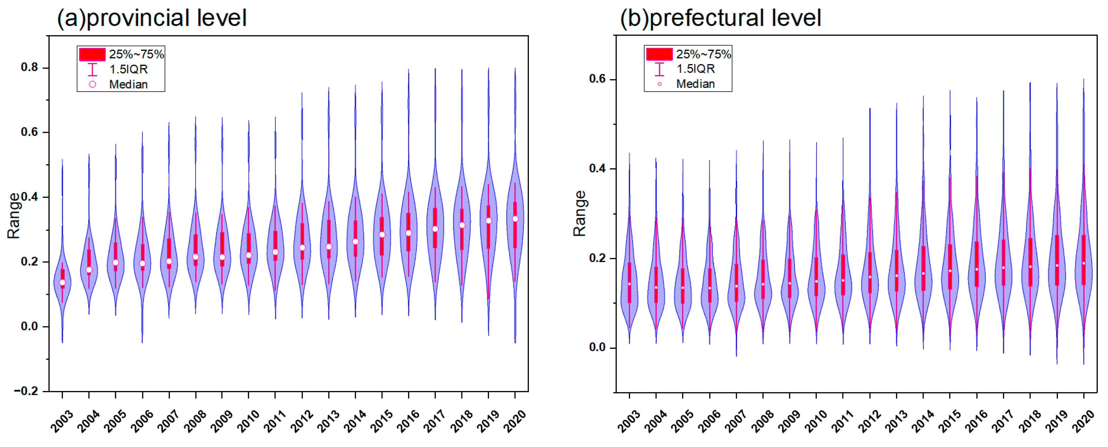
3.1.1. Comparative Analysis of CEP at Two Levels

As shown in Figure 2, CEP at both provincial and prefectural levels exhibited a steady upward trend from 2003 to 2020. Overall, the average CEP at the provincial level was consistently higher than that at the prefectural level, and the rate of increase was also more pronounced at the provincial level. This indicates that spatial scale significantly influences CEP, as evaluations at different administrative levels yield distinct results even when using the same research methods and indicators.

From Figure 3, the spatial differentiation patterns of CEP at both provincial and prefectural levels in 2003, 2012, and 2020 reveal significant variations. The overall spatial pattern indicates higher CEP values in Northeast and Central China, while North and Northwest China exhibit relatively lower CEP. Over the study period, CEP has shown marked improvement, with distinct temporal and spatial variations. For instance, in 2003, provinces such as Heilongjiang, Jilin, and Liaoning in Northeast China recorded lower CEP values. By 2020, these patterns became more pronounced, reflecting significant improvements in CEP across these regions. At the prefectural level, the spatial patterns of CEP exhibit more granular and detailed characteristics compared to the provincial level. Prefectural-level data provide finer insights into regional disparities, revealing localized variations that are often obscured in broader provincial-level analyses.

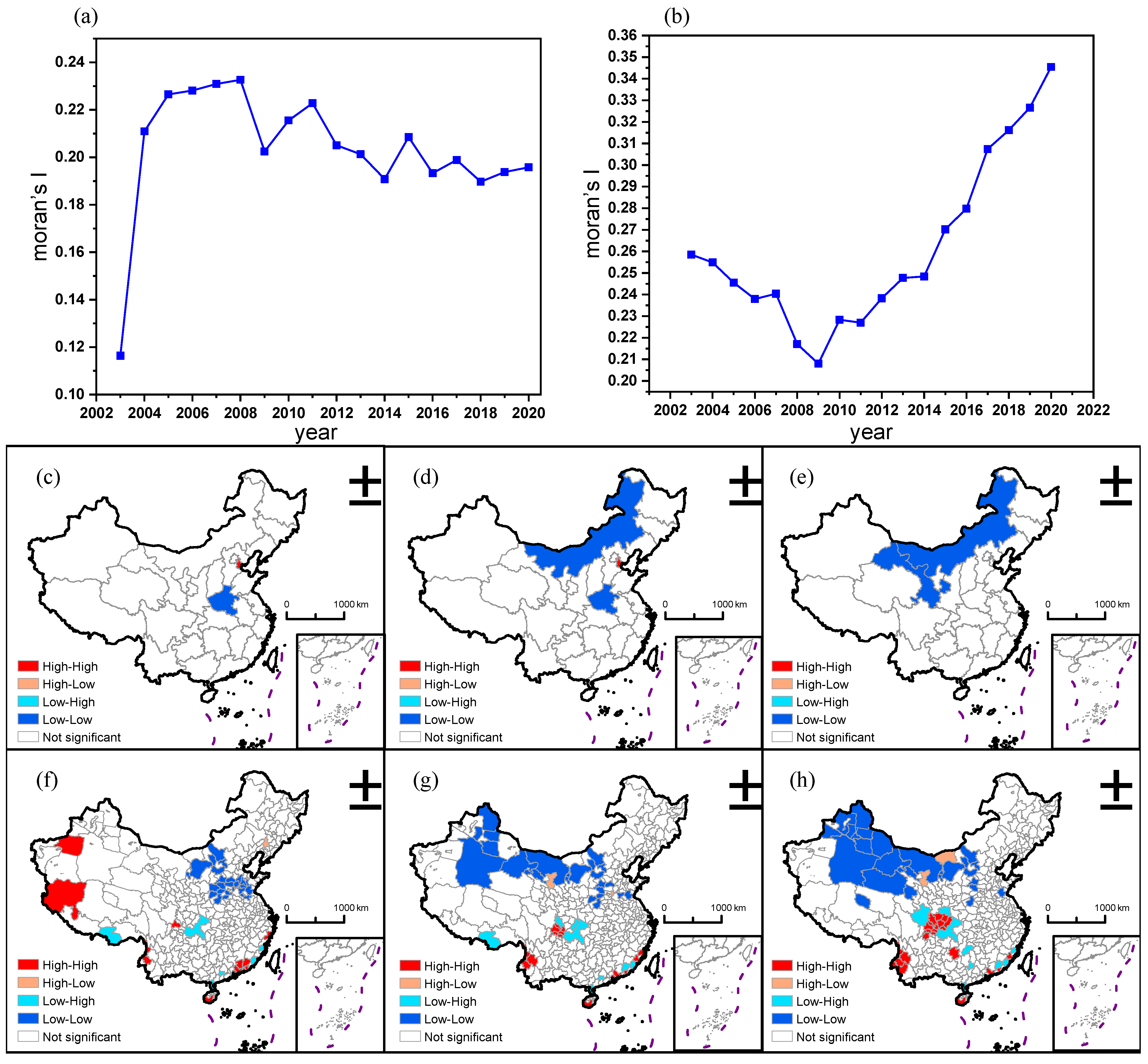
3.1.2. Comparative Spatial Autocorrelation of CEP at Two Levels

Figure 4 illustrates that Moran’s I index for CEP at both provincial and prefectural levels was positive from 2003 to 2020, passing the significance test at the 1% level. This indicates significant spatial positive autocorrelation at both administrative levels. The average Moran’s I index was 0.2035 at the provincial level and 0.2610 at the prefectural level, suggesting stronger spatial autocorrelation at the prefectural level. At the provincial level, Moran’s I increased from 0.1164 in 2003 to 0.2326 in 2008, before gradually declining to 0.1958 in 2020. In contrast, at the prefectural level, Moran’s I initially decreased from 0.2585 in 2003 to 0.2080 in 2009, then rose steadily to 0.3454 in 2020.

Figure 4c–h present the local spatial autocorrelation results for CEP at both levels in 2003, 2012, and 2020. Significant differences in spatial autocorrelation characteristics are observed across levels and years. At the provincial level, spatial clustering was predominantly L–L, concentrated in regions like Inner Mongolia. In 2003, there was 1 H–H cluster and 1 L–L cluster; by 2020, the number of L–L clusters increased to 2, while H–H clusters disappeared. At the prefectural level, clustering types were more diverse, with L–L clusters in Northwest China and H–H clusters in Yunnan and coastal areas. L–H clusters were observed in Fujian, Sichuan, and Chongqing. In 2003, there were 14 H–H, 1 H–L, 7 L–H, and 26 L–L clusters; by 2020, these numbers changed to 23 H–H, 2 H–L, 10 L–H, and 25 L–L clusters. This demonstrates that prefectural-level analysis reveals more detailed spatial patterns, often overlooked in provincial-level studies.

3.2. Comparative Analysis of SDM and DSDM Regression Results

3.2.1. Selection of Model

Given the significant spatial spillover effects of CEP, spatial econometric models were employed. The Lagrange Multiplier (LM) tests confirmed the presence of both spatial lag and spatial error terms at both levels (

Table 2. Spatial econometric model test results for CEP at provincial and prefectural level.

Unit	Test Type	Statistical Value	Unit	Test Type	Statistical Value
Provincial	LM-spatial error	63.936 ***	Prefectural	LM-spatial error	229.24 ***
	Robust-LM-spatial error	42.395 ***		Robust-LM-spatial error	107.18 ***
	LM-spatial lag	23.005 ***		LM-spatial lag	167.2 ***
	Robust-LM-spatial lag	1.4638		Robust-LM-spatial lag	45.136 ***
	Hausman	103.92 ***		Hausman	686.9 ***
	Wald-spatial error	1.143		Wald-spatial error	41.93 ***
	Wald-spatial lag	10.593 **		Wald-spatial lag	63.84 ***

Note: *** means 1% level is significant, ** means 5% level is significant.

). The Hausman test results (103.92 for provincial and 686.9 for prefectural levels) supported the use of fixed effects. The Wald tests indicated that the SDM could not be simplified to SEM or SLM.

3.2.2. Regression Results of SDM and DSDM

Table 3. Regression results of SDM and DSDM of the provincial and prefectural levels.

Variable	Provincial Level				Prefectural Level
	SDM		DSDM		SDM		DSDM
	CEP	Std. Error	CEP	Std. Error	CEP	Std. Error	CEP	Std. Error
CEP_lag			0.8145 ***	0.029			0.8698 ***	0.006
GDPpc	0.003 **	0.001	−0.0009	0.001	0.0001	0.000	0	0.000
lnFAI	−0.0194 **	0.007	−0.0057	0.005	0.0002	0.000	0.0008 **	0.000
lnTEC	−0.0176	0.012	−0.0108	0.010	0.0008	0.001	0.0025 ***	0.001
GDP2	−0.1306 **	0.055	0.0231	0.034	0.0136 **	0.005	0.031 ***	0.005
GDP3	−0.0894	0.066	0.004	0.043	0.0058	0.006	0.0202 ***	0.005
lnFVC	−0.3452 ***	0.049	−0.1506 ***	0.041	0.003	0.003	−0.0025	0.003
NTL	−0.0009	0.001	0.0012	0.001	−0.0008 **	0.000	0.0005	0.000
P_built	−0.4843 ***	0.118	−0.3022 **	0.099	0.0254	0.021	−0.0592 **	0.021
W×CEP	1.1305 ***	0.055	0.1678 **	0.052	1.0834 ***	0.009	0.0831 ***	0.010
rho	−0.7295 ***	0.059	−0.0664	0.062	−1.0594 ***	0.015	0.1283 ***	0.020
R2	0.974		0.988		0.963		0.985
AIC	−966		−1407		2839		−3567
BIC	−924		−1360		2906		−3494

Note: *** means 1% level is significant, ** means 5% level is significant.

presents the regression results of the SDM and DSDM at both provincial and prefectural levels. The SDM reports the regression without incorporating time lag terms, while the DSDM includes time lag terms. The comparison of R², Akaike Information Criterion (AIC) values, and Bayesian Information Criterion (BIC) values indicates that the DSDM, which incorporates time lag terms, provides a better fit. Furthermore, the inclusion of the time lag term (CEP_lag) leads to notable changes in the coefficients of other variables, highlighting the significant influence of temporal dynamics on CEP. Specifically, CEP_lag is statistically significant at both provincial and prefectural levels, exhibiting a positive effect. This suggests that CEP demonstrates strong time-dependent characteristics, with past performance significantly influencing current outcomes.

The spatial interaction term (W×CEP) also shows a positive impact on CEP, passing the 5% significance level test in all cases. This indicates the presence of positive spatial dependence, meaning that CEP in a given region is positively influenced by the CEP of neighboring areas. The stronger spatial spillover effect is observed at the provincial level. This implies that regions with higher CEP levels in their surroundings tend to exhibit higher CEP themselves, reflecting a pattern of regional aggregation in CEP.

The spatial error coefficient (rho) is negative at the provincial level and in the SDM at the prefectural level (−1.0594), while it is positive in the DSDM at the prefectural level (0.1283). Except for the DSDM at the provincial level, all other models pass the 1% significance level test. The results demonstrate that unobserved factors significantly affect CEP in neighboring regions, potentially due to unaccounted spatial spillover effects of key influencing factors.

Regarding specific influencing factors, the impact of GDPpc on CEP is not statistically significant, with relatively low correlation coefficients at both provincial and prefectural levels. LnFAI exhibits a negative effect on CEP at the provincial level but a positive effect at the prefectural level. However, it only passes the 5% significance test in the SDM at the provincial level and in the DSDM at the prefectural level. LnTEC shows a negative effect at the provincial level but a positive effect at the prefectural level, with significance only achieved in the DSDM at the prefectural level (1% significance). GDP2 and GDP3 have a negative effect at the provincial level but exhibit positive effects in other models at both levels. Significance is only achieved at the prefectural level. LnFVC shows significant negative effects at the provincial level but lacks significance at the prefectural level. NTL exhibits significant negative effects at the prefectural level but fails to pass the significance test in other models. P_build demonstrates a significant negative correlation at both provincial and prefectural levels, except for SDM at the prefectural level.

3.3. Comparative Analysis of GTWR Results

3.3.1. Performance of GTWR Results

By constructing the GTWR model at provincial and prefectural levels, this study estimates the spatiotemporal variations in factors influencing CEP. Regression results from OLS and GWR models are also provided, with adjusted R² and AIC used to evaluate model performance (

Table 4. Comparison of model evaluation metrics at provincial and prefectural levels.

Variable	Provincial Level			Prefectural Level
	OLS	GWR	GTWR	OLS	GWR	GTWR
adjusted R2	0.974	0.987	0.986	0.981	0.983	0.983
AIC	−2847	−3269	−3244	−35055	−35862	−35875

). At the provincial level, the GTWR model achieves an adjusted R² of 0.986 and an AIC of −3244, comparable to the GWR model (adjusted R² = 0.987, AIC = −3269). At the provincial level, the GWR model demonstrates slightly better fitting results compared to GTWR, primarily attributable to administrative homogenization effects that attenuate spatiotemporal heterogeneity within provincial boundaries. At the prefectural level, the GTWR model outperforms OLS and GWR, with an adjusted R² of 0.983 and an AIC of −35875, lower than OLS (−35055) and GWR (−35862). The GTWR model better captures the spatiotemporal heterogeneity of CEP influencing factors, making it more suitable for analysis. Therefore, subsequent analyses will use the GTWR model to examine CEP factors at both levels.

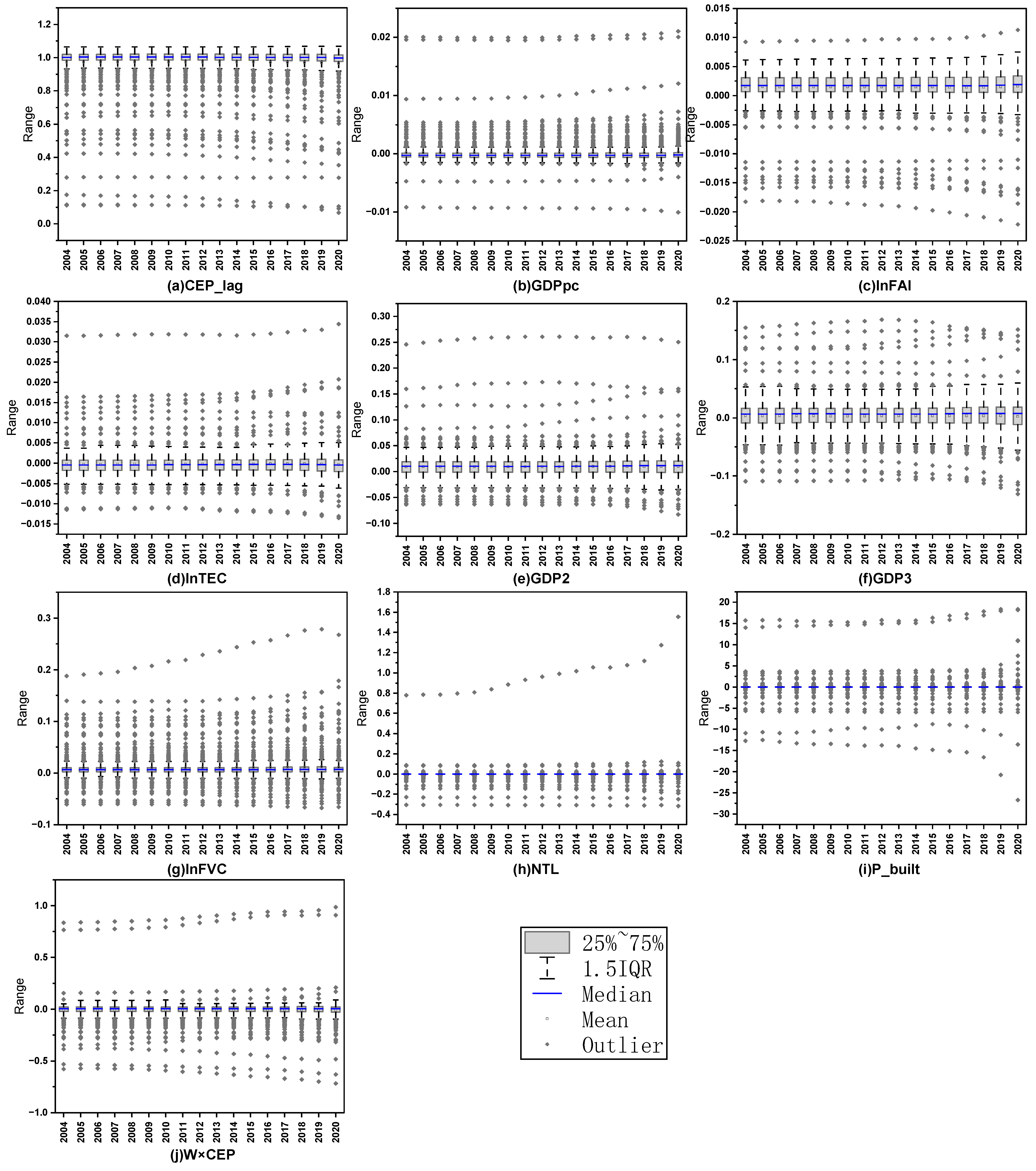
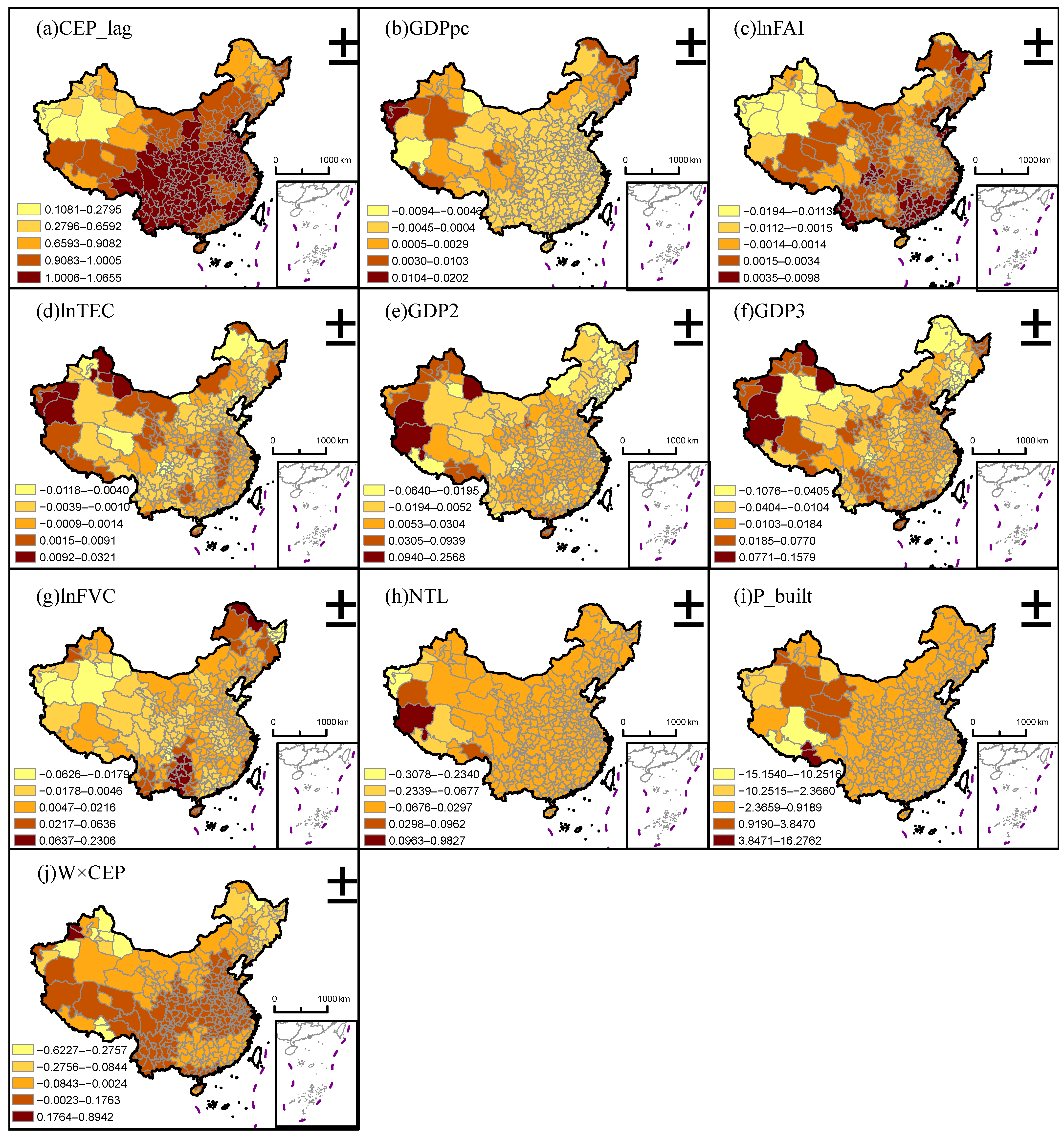
3.3.2. Regression Coefficients of GTWR Model

Table 5. Descriptive statistics of GTWR coefficients.

Scale	Provincial Level					Prefectural Level
Variable	Minimum Value	1/4 Quantile	Median	3/4 Quantile	Maximum Value	Minimum Value	1/4 Quantile	Median	3/4 Quantile	Maximum Value
Intercept	−1.5150	−0.3752	0.0598	0.2092	3.1965	−1.1005	−0.0779	−0.0528	−0.0318	0.5291
CEP_lag	0.1157	0.4241	0.6134	0.7654	1.0173	0.0669	0.9836	1.0024	1.0203	1.0690
GDPpc	−0.0460	−0.0014	0.0012	0.0105	0.0309	−0.0101	−0.0006	−0.0003	0.0001	0.0211
lnFAI	−0.0377	−0.0076	0.0025	0.0198	0.2700	−0.0222	0.0006	0.0018	0.0031	0.0113
lnTEC	−0.3798	−0.0601	−0.0343	−0.0198	0.1300	−0.0135	−0.0018	−0.0004	0.0008	0.0344
GDP2	−0.5380	−0.1279	−0.0052	0.1428	1.0808	−0.0831	−0.0013	0.0103	0.0193	0.2609
GDP3	−0.5312	−0.0376	0.0832	0.1994	1.2186	−0.1309	−0.0096	0.0067	0.0167	0.1686
lnFVC	−1.4613	−0.0462	0.1557	0.3004	0.7783	−0.0677	0.0022	0.0063	0.0110	0.2781
NTL	−3.9850	−0.0272	−0.0024	0.0074	1.2340	−0.3156	−0.0022	−0.0003	0.0003	1.5540
P_built	−628.2600	−0.3580	−0.0744	0.1304	3.6737	−26.6760	−0.0113	0.0025	0.0452	18.4060
W×CEP	−0.4765	−0.0848	0.0539	0.2800	2.0557	−0.7158	−0.0220	0.0047	0.0231	0.9830

presents the descriptive statistics of the regression coefficients derived from GTWR model. The analysis reveals significant variations in the influence of factors such as GDP2, GDP3, and P_built across different administrative levels, with a notably wider distribution range observed at the provincial level compared to the prefectural level. For instance, the coefficient of CEP_lag consistently exhibited positive values, underscoring its strong temporal dependency in affecting CEP. Conversely, GDPpc demonstrated minimal impact at both levels, whereas lnFAI and lnTEC exerted stronger effects at the provincial level.

As illustrated in Figure 5, the temporal variation trends of the GTWR coefficients at the provincial level do not exhibit pronounced time lag differences among the influencing variables. However, notable outliers are observed in GDP2 and GDP3. The CEP_lag coefficient demonstrates an initial increase followed by a decrease, whereas other driving variables maintain relatively stable values over the years. It is noteworthy that the outliers and extreme values of GDPpc, lnFAI, lnTEC, and P_built become increasingly anomalous over time, with NTL and P_built showing particularly drastic fluctuations.

Figure 6 illustrates the temporal variation trends of the GTWR coefficients at the prefectural level. While the values of the driving variables do not exhibit significant annual changes, the degree of data dispersion is more pronounced compared to the provincial level. Notably, the outliers and extreme values of lnFVC and NTL become increasingly anomalous over time.

Figure 7 depicts the spatial variation trends of the GTWR coefficients for provincial units, with the displayed values representing mean coefficient estimates, highlighting distinct spatial differences among the influencing variables. The CEP_lag coefficient is notably higher in Hunan, Hubei, Shanxi, Shaanxi, and Inner Mongolia. GDPpc registers higher values in Yunnan, Tibet, Sichuan, and Heilongjiang. LnFAI is elevated in Ningxia, while lnTEC shows higher values in Tibet and Xinjiang, reflecting a general pattern of higher values in the western regions and lower values in the eastern regions. GDP2 is higher in Jiangsu and Zhejiang but lower in Hubei, Chongqing, and Shanxi. GDP3 is elevated in central Gansu, Shanxi, and Henan. LnFVC is higher in central China, particularly in Hubei and Jiangxi. NTL exhibits higher values in eastern China and lower values in western China. The intense negative effects of P_build are concentrated in Tibet and Qinghai. W×CEP is higher in southwestern and northern China, as well as in Qinghai and Ningxia, but lower in Tibet and Sichuan.

Figure 8 illustrates the spatial variation trends of the GTWR coefficients at the prefectural level, with the displayed values representing mean coefficient estimates, revealing distinct spatial differences among the influencing variables. The CEP_lag coefficient is higher in the central and southwestern regions and lower in the northwestern regions. GDPpc exhibits relatively concentrated values, with minimal spatial differences. LnFAI is higher in Guangdong and lower in western China. The characteristics of lnTEC and GDP2 are somewhat similar, with higher values in Tibet and Xinjiang, reflecting a general pattern of higher values in the west and lower values in the east. GDP3 is higher in Xinjiang and lower in Northeast China. LnFVC is elevated in southwestern China and lower in western China. The spatial variation in NTL is relatively small. P_build exhibits more significant differences in western China and is more concentrated in other regions. W×CEP is higher in central and southwestern China and lower in northern China.

4. Discussion

4.1. Difference in CEP at Two Levels

The analysis of CEP reveals notable differences between provincial and prefectural levels (Figure 3). Over the past 18 years, China’s CEP has consistently exhibited an upward trend at both levels. This study’s findings align with those in study [28], employing the coupling coordination degree model, while diverging from those in study [22], which were obtained through total-factor approaches. The provincial-level CEP is generally higher and demonstrates a larger growth rate compared to the prefectural level. The three sub-indicators of CEP reflect distinct aspects of carbon emissions, and the comprehensive carbon emission performance index not only captures the absolute efficiency of carbon emissions across these dimensions but also evaluates the degree of coordination among them. Consequently, this index provides a more holistic representation of carbon efficiency and the alignment of socio-economic and environmental development.

The global Moran’s I results demonstrate significant spatial autocorrelation in CEP, consistent with the findings of [35], yet reveal distinct local spatial autocorrelation characteristics. Notably, the global Moran’s I results indicate greater significance at the prefectural level compared to the provincial level, although the year of maximum value differs. This implies that spatial scale variations influence Moran’s I of CEP, even when using identical research methods and indicators. Local Moran’s I analysis further highlights that spatial autocorrelation patterns differ significantly across administrative levels, with prefectural-level analyses providing clearer insights into spatial autocorrelation than provincial-level analyses. Thus, while large-scale analyses may neglect small-scale spatial patterns, small-scale analyses are better suited for uncovering regional spatial autocorrelation. By comparing and evaluating the agglomeration patterns of CEP, this study not only offers a foundation for national CEP policy formulation but also provides a scientific reference for local governments to develop differentiated CEP strategies, consistent with conclusions drawn by [60].

4.2. Difference in CEP’s Influencing Factors at Two Levels

From global and local perspectives, this study systematically examines CEP’s influencing factors at both provincial and prefectural levels, demonstrating that while key determinants (GDPpc, lnTEC) maintain statistically significant effects, their spatiotemporal heterogeneity patterns exhibit substantial variations compared to existing research [25,28,35], particularly in the specific characteristics of spatial–temporal consistency.

Global regression results reveal that socioeconomic and land-use factors significantly impact CEP, with CEP exhibiting notable spatial spillover effects. However, not all indicators show significant correlations with CEP at both levels. For instance, lnFVC has a more substantial impact on CEP at the provincial level, while its effect is insignificant at the prefectural level. At the provincial level, the influencing factors are ranked as CEP_lag > P_built > W×CEP > lnFVC, whereas at the prefectural level, the ranking is CEP_lag > rho > W×CEP > P_built. Notably, socioeconomic factors such as GDP2, GDP3, and lnTEC are statistically significant at the prefectural level, indicating that these factors play a more pronounced role at the prefectural level compared to the provincial level.

The local regression results highlight significant temporal and spatial heterogeneity in the impacts of influencing factors on CEP across provincial and prefectural levels. The GTWR model, which integrates temporal and spatial dimensions, proves particularly effective in capturing these variations, aligning with existing research findings [4]. Land-use factors, such as P_built and NTL, exhibit anomalous distributions, indicating unstable spatiotemporal effects on CEP, while socioeconomic factors show more consistent patterns. lnFVC and W×CEP exhibit the most pronounced spatial differences across the two scales. Provincial-level units, with stronger administrative and economic powers, influence CEP through large-scale policies, whereas prefectural-level units focus on localized urban development. This leads to distinct influencing factors at each level. The spatial heterogeneity of CEP also means that the direction and intensity of influencing factors can vary significantly across scales, necessitating multi-scale analyses and tailored policies to address regional disparities effectively.

4.3. Policy Implications

The comprehensive evaluation of CEP can more fairly and objectively reflect a region’s carbon performance and level of low-carbon development, offering a novel approach for determining regional carbon emission reduction responsibilities. The comprehensive carbon emission performance index provides a scientific reference for assigning such responsibilities. Our findings have several implications for policymakers to develop reliable CEP mitigation strategies in China: (1) At both provincial and prefectural scales, CEP exhibits significant spatial spillover effects, indicating a strong interdependence among neighboring regions. Empirical evidence suggests that enhancing CEP in a given region can positively influence CEP improvements in adjacent areas, with particularly pronounced effects observed at the prefectural level. These findings underscore the importance of fostering interjurisdictional collaboration and institutionalizing coordinated governance mechanisms to optimize regional environmental performance. (2) Economic Structure Optimization: The higher correlation between the secondary industry’s proportion and CEP at the provincial level underscores the importance of optimizing economic structures, particularly in provinces reliant on energy-intensive industries. Policymakers should prioritize upgrading traditional industries and supporting low-emission sectors such as services and finance. (3) Land-Use Considerations: Future carbon-related policy formulation should systematically integrate land-use optimization strategies by coordinating lnFVC enhancement, NTL regulation, and P_built control to achieve synergistic carbon emission reduction and sustainable spatial planning outcomes. (4) Differentiated Policies: Given the heterogeneous and multiscale characteristics of CEP, policymakers should adopt a “proceed in light of local conditions” strategy. Tailored policies based on regional differences—such as urban type, development stage, economic scale, and technical level—are more effective than uniform approaches. For cities or factors with high spatial differentiation, flexible and differentiated low-carbon policies are recommended, while regions with low spatial differentiation may benefit from more standardized policies.

5. Conclusions

To support China’s “3060” dual-carbon goals, this study employs a coupling coordination degree model to measure CEP and conducts a systematical comparative analysis of the global and local effects of influencing factors at both provincial and municipal levels using SDM, DSDM, and GTWR models. The results demonstrate that:

(1)

From 2003 to 2020, CEP exhibited a steady upward trend at both levels, with the average CEP at the provincial level consistently higher than that at the prefectural level. Higher CEP values were found in Northeast and Central China, while North and Northwest China exhibited relatively lower CEP. Moran’s I indices of CEP at both levels were positive, and the prefectural-level Moran’s I was higher than the provincial-level Moran’s I. Provincial-level Local Moran’s I identified 1–2 L–L clusters during 2003–2020, while the prefectural-level Local Moran’s I revealed 14–23 H–H(26–25 L–L) clusters during 2003–2020, demonstrating significantly richer spatial patterns at prefectural level.

(2)

The contributions of influencing factors to CEP vary significantly between provinces and prefectural cities. The spatial interaction term (W×CEP) also shows a positive impact on CEP, passing the 5% significance level test in all cases. From a global perspective based on the DSDM, the terms are ranked as CEP_lag > P_built > W×CEP > lnFVC, whereas at the prefectural level, the ranking is CEP_lag > rho > W×CEP > P_built. Notably, socioeconomic factors such as GDP2 and GDP3 are more statistically significant at the prefectural level.

(3)

The local regression results demonstrate substantial spatiotemporal heterogeneity in the factors influencing CEP across both provincial and prefectural levels. The distributions of GDPpc, lnFAI, lnTEC, and P_built exhibit increasingly anomalous outliers and extreme values over time, with NTL and P_built displaying particularly pronounced fluctuations. The GTWR coefficients for CEP_lag, lnFVC, and W×CEP show the most marked scale-dependent variations, with significant differences observed between provincial and prefectural levels. Furthermore, land-use variables (P_built and NTL) manifest irregular spatial patterns, indicating their non-stationary impacts on CEP across space and time.

This study has several limitations. First, although the study covers 18 years, a longer time span could provide more accurate insights into the spatiotemporal characteristics and influencing factors of CEP. Second, some influencing factors, such as energy consumption structure and urbanization, are not fully considered due to limited city-level data. Future research should focus on refining indicator selection to better analyze CEP’s impact mechanisms. Third, the binary weight matrix used in spatial autocorrelation analysis does not fully capture the frictional coefficients of economy, trade, labor, and capital flow, which may influence CEP.

References

1. Joseph, V.R.; Mustaffa, N.K. Carbon emissions management in construction operations: A systematic review. Eng. Constr. Archit. Manag. 2023, 30, 1271–1299. [Google Scholar] [CrossRef]
2. Miao, X.; Feng, E.H.; Siu, Y.L.; Li, S.S.; Wong, C.W.Y. Can China’s carbon intensity constraint policies improve carbon emission performance? Evidence from regional carbon emissions. J. Environ. Manag. 2023, 348, 119268. [Google Scholar] [CrossRef]
3. Lu, H.Y.; Meng, H.L.; Lu, C.Z.; Shang, D.; Wang, D.; Jin, H. The mechanism for selecting low carbon urban experimentation cases in the literature and its impact on carbon emission performance. J. Clean. Prod. 2023, 420, 138191. [Google Scholar] [CrossRef]
4. Li, W.; Ji, Z.; Dong, F. Spatio-temporal evolution relationships between provincial CO2 emissions and driving factors using geographically and temporally weighted regression model. Sustain. Cities Soc. 2022, 81, 103836. [Google Scholar] [CrossRef]
5. Shan, Y.; Guan, Y.; Hang, Y.; Zheng, H.; Li, Y.; Guan, D.; Li, J.; Zhou, Y.; Li, L.; Hubacek, K. City-level emission peak and drivers in China. Sci. Bull. 2022, 67, 1910–1920. [Google Scholar] [CrossRef]
6. Yang, J.; Feng, X.; Li, Y.; He, C.; Wang, S.; Li, F. How Does Urban Scale Influence Carbon Emissions? Land 2024, 13, 1254. [Google Scholar] [CrossRef]
7. Gao, Z.; Xia, E.; Lin, S.; Xu, J.; Tao, C.; Yu, C. Carbon emission efficiency and regional synergistic peaking strategies in Beijing-Tianjin-Hebei region. Carbon Neutrality 2024, 3, 19. [Google Scholar] [CrossRef]
8. Li, J.; Cheng, Z. Study on total-factor carbon emission efficiency of China’s manufacturing industry when considering technology heterogeneity. J. Clean. Prod. 2020, 260, 121021. [Google Scholar] [CrossRef]
9. Wang, S.; Wang, H.; Zhang, L.; Dang, J. Provincial Carbon Emissions Efficiency and Its Influencing Factors in China. Sustainability 2019, 11, 2355. [Google Scholar] [CrossRef]
10. Zhou, Z.; Liu, C.; Zeng, X.; Jiang, Y.; Liu, W. Carbon emission performance evaluation and allocation in Chinese cities. J. Clean. Prod. 2018, 172, 1254–1272. [Google Scholar] [CrossRef]
11. Zhou, A.; Li, J. Impact of policy combinations on carbon emission performance: Evidence from China. Clean Technol. Environ. Policy 2024, 26, 3069–3088. [Google Scholar] [CrossRef]
12. Zhao, Z.Y.; Zhao, Y.H.; Shi, X.P.; Zheng, L.; Fan, S.A.; Zuo, S.M. Green innovation and carbon emission performance: The role of digital economy. Energy Policy 2024, 195, 114344. [Google Scholar] [CrossRef]
13. Zhao, M.; Sun, T.; Feng, Q. A study on evaluation and influencing factors of carbon emission performance in China’s new energy vehicle enterprises. Environ. Sci. Pollut. Res. Int. 2021, 28, 57334–57347. [Google Scholar] [CrossRef] [PubMed]
14. Xiao, Y.; Ma, D.; Zhang, F.; Zhao, N.; Wang, L.; Guo, Z.; Zhang, J.; An, B.; Xiao, Y. Spatiotemporal differentiation of carbon emission efficiency and influencing factors: From the perspective of 136 countries. Sci. Total Environ. 2023, 879, 163032. [Google Scholar] [CrossRef]
15. Li, S.; Diao, H.; Wang, L.; Li, L. A complete total-factor CO2 emissions efficiency measure and “2030•60 CO2 emissions targets” for Shandong Province, China. J. Clean. Prod. 2022, 360, 132230. [Google Scholar] [CrossRef]
16. He, J.; Yang, J. Spatial–Temporal Characteristics and Influencing Factors of Land-Use Carbon Emissions: An Empirical Analysis Based on the GTWR Model. Land 2023, 12, 1506. [Google Scholar] [CrossRef]
17. Gao, Z.; Li, S.; Cao, X.; Li, Y. Carbon Emission Intensity Characteristics and Spatial Spillover Effects in Counties in Northeast China: Based on a Spatial Econometric Model. Land 2022, 11, 753. [Google Scholar] [CrossRef]
18. Wang, S.; Fang, C.; Guan, X.; Pang, B.; Ma, H. Urbanisation, energy consumption, and carbon dioxide emissions in China: A panel data analysis of China’s provinces. Appl. Energy 2014, 136, 738–749. [Google Scholar] [CrossRef]
19. Zheng, Y.; Sun, X.; Zhang, C.; Wang, D.; Mao, J. Can Emission Trading Scheme Improve Carbon Emission Performance? Evidence From China. Front. Energy Res. 2021, 9, 759572. [Google Scholar] [CrossRef]
20. Ma, R.; Zhang, Z.; Lin, B. Evaluating the synergistic effect of digitalization and industrialization on total factor carbon emission performance. J. Environ. Manag. 2023, 348, 119281. [Google Scholar] [CrossRef]
21. Feng, X.H.; Lin, X.L.; Li, Y.; Yang, J.Y.; Yu, E.; Lei, K.G. Spatial association network of carbon emission performance: Formation mechanism and structural characteristics. Socio-Econ. Plan. Sci. 2024, 91, 101792. [Google Scholar] [CrossRef]
22. Zhang, X.; Zhou, J.; Wu, R.; Wang, S. Spatial network analysis and driving forces of urban carbon emission performance: Insights from Guangdong Province. Sci. Total Environ. 2024, 951, 175538. [Google Scholar] [CrossRef]
23. Wang, S.; Wang, Z.; Fang, C. Evolutionary characteristics and driving factors of carbon emission performance at the city level in China. Sci. China Earth Sci. 2022, 65, 1292–1307. [Google Scholar] [CrossRef]
24. Li, Y.; Hou, W.; Zhu, W.; Li, F.; Liang, L. Provincial carbon emission performance analysis in China based on a Malmquist data envelopment analysis approach with fixed-sum undesirable outputs. Ann. Oper. Res. 2021, 304, 233–261. [Google Scholar] [CrossRef]
25. Zhao, Z.; Ren, J.; Liu, Z. How Does Urbanization Affect Carbon Emission Performance? Evidence from 282 Cities in China. Sustainability 2023, 15, 15498. [Google Scholar] [CrossRef]
26. Dong, G.L.; Huang, Y.; Zhang, Y.L.; Zhao, D.Q.; Wang, W.J.; Liao, C.P. Drivers of carbon intensity decline during the new economic normal: A multilevel decomposition of the Guangdong case. J. Clean. Prod. 2024, 437, 140631. [Google Scholar] [CrossRef]
27. Lv, Y.; Liu, J.; Cheng, J.; Andreoni, V. The persistent and transient total factor carbon emission performance and its economic determinants: Evidence from China’s province-level panel data. J. Clean. Prod. 2021, 316, 128198. [Google Scholar] [CrossRef]
28. Guo, Y.; Li, X.; Li, S. Green Technology Innovation and Carbon Emission Performance of the Middle Reaches of the Yangtze River Urban Agglomeration: Mechanism and Spatio-Temporal Evolution. Energies 2024, 17, 5274. [Google Scholar] [CrossRef]
29. Meng, Q.G.; Chen, X.L.; Wang, H.; Shen, W.F.; Duan, P.X.; Liu, X.Y. Spatiotemporal evolution and driving factors of the synergistic effects of pollution control and carbon reduction in China. Ecol. Indic. 2025, 170, 113103. [Google Scholar] [CrossRef]
30. Li, L.; Li, J.; Peng, L.; Wang, X.; Sun, S. Spatiotemporal evolution and influencing factors of land-use emissions in the Guangdong-Hong Kong-Macao Greater Bay Area using integrated nighttime light datasets. Sci. Total Environ. 2023, 893, 164723. [Google Scholar] [CrossRef]
31. Zhao, Z.; Yuan, T.; Shi, X.; Zhao, L. Heterogeneity in the relationship between carbon emission performance and urbanization: Evidence from China. Mitig. Adapt. Strateg. Glob. Change 2020, 25, 1363–1380. [Google Scholar] [CrossRef] [PubMed]
32. Liu, D.; Liu, W.; He, Y. How Does the Intensive Use of Urban Construction Land Improve Carbon Emission Efficiency?—Evidence from the Panel Data of 30 Provinces in China. Land 2024, 13, 2133. [Google Scholar] [CrossRef]
33. Xu, Y.; Liu, Z.; Walker, T.R.; Adams, M.; Dong, H. Spatio-temporal patterns and spillover effects of synergy on carbon dioxide emission and pollution reductions in the Yangtze River Delta region in China. Sustain. Cities Soc. 2024, 107, 105419. [Google Scholar] [CrossRef]
34. Wang, S.; Gao, S.; Huang, Y.; Shi, C. Spatiotemporal evolution of urban carbon emission performance in China and prediction of future trends. J. Geogr. Sci. 2020, 30, 757–774. [Google Scholar] [CrossRef]
35. Zhang, W.; Liu, X.; Zhao, S.; Tang, T. Does green finance agglomeration improve carbon emission performance in China? A perspective of spatial spillover. Appl. Energy 2024, 358, 122561. [Google Scholar] [CrossRef]
36. Qiao, W.; Xie, Y.; Liu, J.; Huang, X. The Impacts of Urbanization on Carbon Emission Performance: New Evidence from the Yangtze River Delta Urban Agglomeration, China. Land 2024, 14, 12. [Google Scholar] [CrossRef]
37. Wen, H.; Yu, H.; Nghiem, X.-H. Impact of urban sprawl on carbon emission efficiency: Evidence from China. Urban Clim. 2024, 55, 101986. [Google Scholar] [CrossRef]
38. Li, S.; Sun, Z.L.; Wen, R.B.; Yang, H.; Li, J.J.; Chen, T.T.; Zheng, Y.S.; Zhu, N. Spatiotemporal patterns and the influence mechanism of urban landscape pattern on carbon emission performance: Evidence from Chinese cities. Sustain. Cities Soc. 2025, 118, 106042. [Google Scholar] [CrossRef]
39. Meng, Q.; Li, B.; Zheng, Y.; Zhu, H.; Xiong, Z.; Li, Y.; Li, Q. Multi-Scenario Prediction Analysis of Carbon Peak Based on STIRPAT Model-Take South-to-North Water Diversion Central Route Provinces and Cities as an Example. Land 2023, 12, 2035. [Google Scholar] [CrossRef]
40. Jiang, P.; Gong, X.; Yang, Y.; Tang, K.; Zhao, Y.; Liu, S.; Liu, L. Research on spatial and temporal differences of carbon emissions and influencing factors in eight economic regions of China based on LMDI model. Sci. Rep. 2023, 13, 7965. [Google Scholar] [CrossRef]
41. Wu, G.; Cui, S.; Wang, Z. The role of renewable energy investment and energy resource endowment in the evolution of carbon emission efficiency: Spatial effect and the mediating effect. Environ. Sci. Pollut. Res. Int. 2023, 30, 84563–84582. [Google Scholar] [CrossRef] [PubMed]
42. Wang, B.; Zhang, C.H. Toward transition and upgrading: Carbon emission performance and its influencing factors in China’s energy-intensive industries. Environ. Dev. Sustain. 2025, 1–29. [Google Scholar] [CrossRef]
43. Liang, X.; Min, F.; Xiao, Y.; Yao, J. Temporal-spatial characteristics of energy-based carbon dioxide emissions and driving factors during 2004–2019, China. Energy 2022, 261, 124965. [Google Scholar] [CrossRef]
44. Wang, Y.; Chen, W.; Kang, Y.; Li, W.; Guo, F. Spatial correlation of factors affecting CO2 emission at provincial level in China: A geographically weighted regression approach. J. Clean. Prod. 2018, 184, 929–937. [Google Scholar] [CrossRef]
45. He, Y.L.; Zhang, X.H.; Pu, N.; Wu, C.Y.; Tang, W. Spatiotemporal pattern and driving factors of atmospheric CO2 concentrations based on satellite remote sensing from 2001 to 2022 in central Yunnan plateau. Ecol. Indic. 2025, 173, 113371. [Google Scholar] [CrossRef]
46. Gao, S.; Sun, D.Q.; Wang, S.J. Do development zones increase carbon emission performance of China’s cities? Sci. Total Environ. 2023, 863, 160784. [Google Scholar] [CrossRef] [PubMed]
47. Liu, Q.; Wu, S.; Lei, Y.; Li, S.; Li, L. Exploring spatial characteristics of city-level CO2 emissions in China and their influencing factors from global and local perspectives. Sci. Total Environ. 2021, 754, 142206. [Google Scholar] [CrossRef]
48. Zhu, K.; Tu, M.; Li, Y. Did Polycentric and Compact Structure Reduce Carbon Emissions? A Spatial Panel Data Analysis of 286 Chinese Cities from 2002 to 2019. Land 2022, 11, 185. [Google Scholar] [CrossRef]
49. Ma, Y.; Zhang, Z.; Yang, Y. Calculation of carbon emission efficiency in China and analysis of influencing factors. Environ. Sci. Pollut. Res. 2023, 30, 111208–111220. [Google Scholar] [CrossRef]
50. Jiang, F.; Chen, B.; Li, P.; Jiang, J.; Zhang, Q.; Wang, J.; Deng, J. Spatio-temporal evolution and influencing factors of synergizing the reduction of pollution and carbon emissions—Utilizing multi-source remote sensing data and GTWR model. Environ. Res. 2023, 229, 115775. [Google Scholar] [CrossRef]
51. Xu, Q.Y.; Yao, L.; Shi, K.F.; Zhou, W.; Tang, X.G. Spatiotemporal analysis of the impact of green finance on carbon dioxide emissions based on panel data of cities in China. Int. J. Digit. Earth 2025, 18, 2457969. [Google Scholar] [CrossRef]
52. Xiang, W.M.; Liu, T.; Gan, L. Spatiotemporal heterogeneity of the influence of industrial linkage on building carbon emission. J. Build. Eng. 2025, 100, 111772. [Google Scholar] [CrossRef]
53. Wang, Z.P.; Li, K.M. Can green finance exorcize the resource curse in China’s resource-based cities? A geographically and temporally weighted regression (GTWR) analysis. J. Environ. Manag. 2025, 375, 124184. [Google Scholar] [CrossRef]
54. Abudureheman, M.; Yiming, A. The impact of energy-saving R&D on urban carbon emission performance: Evidence from 218 prefecture-level cities in China. Front. Environ. Sci. 2024, 12, 1385363. [Google Scholar] [CrossRef]
55. You, X.J.; Chen, Z.Q. Interaction and mediation effects of economic growth and innovation performance on carbon emissions: Insights from 282 Chinese cities. Sci. Total Environ. 2022, 831, 154910. [Google Scholar] [CrossRef] [PubMed]
56. Song, M.; Gao, Y.; Zhang, L.; Dong, F.; Zhao, X.; Wu, J. Spatiotemporal evolution and driving factors of carbon emission efficiency of resource-based cities in the Yellow River Basin of China. Environ. Sci. Pollut. Res. 2023, 30, 96795–96807. [Google Scholar] [CrossRef]
57. Li, J.; Zhou, Y.P.; Chen, H.Y. Measurement, influencing factors and prediction on carbon emission performance of countries along the Belt and Road. Clean Technol. Environ. Policy 2024, 26, 821–838. [Google Scholar] [CrossRef]
58. Wang, X.; Yu, H.; Wu, Y.; Zhou, C.; Li, Y.; Lai, X.; He, J. Spatio-Temporal Dynamics of Carbon Emissions and Their Influencing Factors at the County Scale: A Case Study of Zhejiang Province, China. Land 2024, 13, 381. [Google Scholar] [CrossRef]
59. Liu, Q.; Song, J.; Dai, T.; Shi, A.; Xu, J.; Wang, E. Spatio-temporal dynamic evolution of carbon emission intensity and the effectiveness of carbon emission reduction at county level based on nighttime light data. J. Clean. Prod. 2022, 362, 132301. [Google Scholar] [CrossRef]
60. Shi, K.; Yu, B.; Zhou, Y.; Chen, Y.; Yang, C.; Chen, Z.; Wu, J. Spatiotemporal variations of CO2 emissions and their impact factors in China: A comparative analysis between the provincial and prefectural levels. Appl. Energy 2019, 233–234, 170–181. [Google Scholar] [CrossRef]
61. Dai, B.-t.; Zhi, D.-d.; Ren, L.; Kong, W.; Wang, S.-j. Research on misuses and modification of coupling coordination degree model in China. J. Nat. Resour. 2021, 36, 793–810. [Google Scholar] [CrossRef]
62. Jianmin, Z.; Yang, Y.; Jingyuan, H.; Xiaoxuan, K. Can urbanization improve carbon performance? Front. Environ. Sci. 2024, 12, 1431324. [Google Scholar] [CrossRef]
63. Zhang, H.; Geng, C.; Wei, J. Coordinated development between green finance and environmental performance in China: The spatial-temporal difference and driving factors. J. Clean. Prod. 2022, 346, 131150. [Google Scholar] [CrossRef]
64. Espoir, D.K.; Sunge, R. CO2 emissions and economic development in Africa: Evidence from a dynamic spatial panel model. J. Env. Manag. 2021, 300, 113617. [Google Scholar] [CrossRef]
65. Chen, X.; He, Q.; Ye, T.; Liang, Y.; Li, Y. Decoding spatiotemporal dynamics in atmospheric CO2 in Chinese cities: Insights from satellite remote sensing and geographically and temporally weighted regression analysis. Sci. Total Environ. 2024, 908, 167917. [Google Scholar] [CrossRef]
Figure 1. The study areas of China, showing two administrative levels: provinces and prefectures. Note: The base map was plotted using Standard Map GS (2024) 0650 (http://bzdt.ch.mnr.gov.cn/, accessed on 1 January 2025) approved by China’s Ministry of Natural Resources, with no modifications to the original geographic boundaries, and the same below.
Land 14 01146 g001
Figure 2. Statistical trends of CEP at the provincial and prefectural levels from 2003 to 2020.
Land 14 01146 g002
Figure 3. Spatial distribution of CEP at the provincial and prefectural levels in 2003, 2012, and 2020: (a) provincial level in 2003, (b) provincial level in 2012, (c) provincial level in 2020, (d) prefectural level in 2003, (e) prefectural level in 2012, and (f) prefectural level in 2020.
Land 14 01146 g003
Figure 4. Spatial autocorrelation results of CEP: (a) Global Moran’s I index at the provincial level, (b) Global Moran’s I index at the prefectural level, (ce) LISA clusters at provincial level (2003, 2012, 2020), (fh) LISA clusters at prefectural level (2003, 2012, 2020).
Land 14 01146 g004
Figure 5. Time series variation trend of GTWR coefficient at the provincial level.
Land 14 01146 g005
Figure 6. Time series variation trend of GTWR coefficient at the prefectural level.
Land 14 01146 g006
Figure 7. Spatial variation trend of GTWR coefficient at the provincial level.
Land 14 01146 g007
Figure 8. Spatial variation trend of GTWR coefficient at the prefectural level.
Land 14 01146 g008