Regional Differences in Agricultural Carbon Emissions in China: Measurement, Decomposition, and Influencing Factors

Abstract

As one of the major sources of carbon emissions, the significant spatial disparities in agricultural carbon emissions (ACE) pose a serious challenge to coordinated regional carbon reduction efforts. In order to precisely identify the sources of these ACE differences, this study estimates the ACE of China from 2005 to 2020 across four main emission sources and applies the bidimensional decomposition method of the Gini coefficient to measure and decompose their spatial disparities. Finally, the key factors driving ACE disparities are analyzed using the Quadratic Assignment Procedure (QAP). The results show that China’s total ACE initially declined, followed by an upward trend over the study period. Spatially, emissions were higher in eastern regions compared to western regions, and higher in southern regions compared to northern regions. The differences in paddy field emissions between the central and western regions were identified as the primary contributor to east–west disparities, while differences in agricultural materials emissions between northern and southern regions were the dominant source of north–south disparities. Furthermore, regional differences in agricultural development levels and mechanization capacity were found to be the strongest drivers of spatial ACE disparities. This study provides empirical evidence for formulating region-specific and source-targeted carbon reduction policies. Our findings highlight the importance of addressing regional imbalances, particularly in paddy field management and agricultural material usage, to promote more coordinated and sustainable agricultural carbon reduction across China.

1. Introduction

Human development is threatened by greenhouse gas (GHG) emissions, which lead to global warming [1,2]. Amongst these emissions, the unregulated release of carbon dioxide jeopardizes social health [3]. Governments worldwide have prioritized the reduction in carbon dioxide emissions as a central strategy to combat global warming and mitigate GHG emissions [4]. This commitment was reinforced during the 2015 Paris Climate Conference, where China announced it would decrease its carbon intensity by 60% in 2030. To strengthen its dedication, China introduced a dual carbon goal during the 2020 United Nations Climate Conference [5]. This goal aims to achieve a carbon emission peak by 2030 and attain carbon neutrality by 2060 [6]. However, as one of the largest carbon dioxide emitters [7], China faces the critical challenge of equitably distributing the carbon reduction burden across various regions and sectors [8].

Agricultural carbon emissions (ACE) contribute to 23% of anthropogenic GHG emissions, representing the second largest source worldwide [9]. As an agricultural and carbon-emitting country, China’s agricultural activities emissions contribute to a substantial 11% of the general emissions [10], which is well above the global average. As the abuse of agricultural chemicals and fertilizers continues, carbon emissions from the agricultural sector will increase continuously [11]. Accordingly, the urgency of reducing carbon emissions within the agricultural domain is undeniable.

China has implemented a variety of carbon emission reduction measures aimed at the agricultural sector, thereby producing notable positive results [12]. However, there are obvious differences in planting structures and environmental systems in different regions [13], leading to significant spatial differences in ACE [14]. In this context, accurate assessment of ACE and exploration of the spatial differences, along with identifying key factors, are crucial prerequisites for formulating policies. This will encourage low-carbon and environmentally sustainable agricultural practices, ultimately contributing to carbon neutrality within the agricultural sector. The ACE in this study represents the carbon equivalent converted from three major types of GHG emissions arising directly or indirectly from agricultural activities. These include methane (CH₄) emissions from rice paddy anaerobic fermentation, enteric fermentation in ruminants, and manure management, along with nitrous oxide (N₂O) emissions from fertilizer application, soil tillage, organic fertilizer decomposition, and open-air manure storage.

The contributions of this article are threefold and significantly advance the understanding of ACE spatial differences. First, this study addresses the complexity of ACE spatial variation by categorizing into four major regions along the east–west axis and two regions along the north–south axis. Unlike previous studies that relied on a simple east–west division, this refined classification fills a critical research gap, especially regarding north–south variations. Second, this study employs the Gini ratio bidimensional decomposition method to analyze the sources of ACE differences. This method integrates traditional regional variation sources with endogenous factors, allowing for a more precise identification of these sources. It represents an innovative and practical approach that can be extended to various application scenarios. Third, beyond examining internal factors affecting spatial differences, this study applies the Quadratic Assignment Procedure (QAP) to analyze external influences on ACE disparities. This method provides a novel perspective on addressing spatial differences in ACE and offers empirical support for designing region-specific strategies for agricultural carbon reduction. These contributions collectively provide a new framework for understanding and managing ACE in China.

The remaining content of this study is structured as follows: Section 2 is a literature review. Section 3 introduces the methodology. Section 4 displays the research results and discussion. Section 5 presents the conclusions, policy implications, and limitations.

2. Literature Review

2.1. Measurement of ACE

The complexities and diversities of agricultural production activities result in multiple sources of ACE [15]. Discrepancies amongst the various methods used to estimate carbon emissions can lead to differing outcomes. West and Marland [16] computed carbon cycling emissions in the United States’ agricultural sector by considering four aspects: fertilizers, pesticides, irrigation, and breeding, stressing the significance of CH₄ emissions in agricultural production. Johnson et al. [17] emphasized that livestock emissions, enteric fermentation, and manure management significantly contribute to CH₄ emissions, acknowledging the significance of N₂O as a potent GHG. Based on that, Reay et al. [18] proposed improvements to measurement and estimation methodologies for agricultural N₂O emissions. Guan et al. [19] calculated China’s ACE from two aspects: carbon emissions generated by agricultural material input in the process of agricultural production and carbon emissions caused by farmland change.

2.2. Spatial Differences and Sources of ACE

Diverse regions of China display substantial variations in terms of resource endowments, agricultural structures, economies, and technologies [20,21]. These differences influence the variations in ACE [22]. Measuring, estimating, and reconciling regional ACE differences are critical to driving a sustainable trajectory for China [20].

Zhao et al. [23] identified that the high-ACE regions are mainly concentrated in the northeast and western regions with vast cultivated land. Analyzing spatial differences through the perspective of carbon sources, Liu and Yang [14] observed that eastern China displayed favorable progress in adopting low-carbon agricultural practices, whereas the central region experienced an increase in ACE. He et al. [24] revealed that carbon emissions from crop cultivation were primarily concentrated in the middle Yangtze River, whereas LBE primarily originated from Inner Mongolia. By analyzing the spatial distribution structure of urban carbon emissions, Zhang et al. [25] found that central urban areas and suburban industrial areas are the main sources.

Numerous scholars have used the Theil index for decomposing the spatial differences in ACE and suggested that inter-regional differences predominantly contribute to the overall differences [26,27]. Within the regions, regional differences are most significant in the eastern region [28]. Furthermore, other researchers have chosen the Dagum Gini coefficient to decompose the overall difference, with inter-regional difference still being the main source of overall difference [29]. Han et al. [30] discovered substantial differences amongst provinces in terms of the structure and intensity of ACE, with inter-regional differences consistently emerging as the major source. Qin et al. [31] found that the intra-regional and inter-regional differences were narrowing. Similarly, Cui et al. [32] discovered that despite the trend of narrowing inter-regional differences, they are still the main source of overall difference in ACE per capita.

2.3. Key Factors of ACE

Exploring the key factors of ACE is fundamental for devising strategies to reduce such emissions. Sarkar et al. [33] revealed that driving innovation in energy and biotechnology can reduce ACE in Canada. Similarly, Zhang et al. [34] discovered that agricultural energy consumption negatively affects ACE, whereas agricultural economic growth exerts a positive effect. Wei et al. [35] combined the Tapio decoupling model with the Stochastic Impacts by Regression on Population, Affluence, and Technology model and found that rural urbanization rate and per capita consumption expenditure had a negative impact on carbon emissions. Furthermore, Han et al. [36] identified economic development and the scale of agricultural expansion as primary driving forces of ACE, and agricultural subsidies and technological advancements emerged as key factors that reduce ACE. However, Su et al. [37] found that improvements in agricultural development showed no significant effect on ACE. Given that the influence of each factor varies across regions, considering the spatial characteristics of driving forces is necessary [38].

We reviewed the literature similar to this study (

Table 1. Existing reference ACE measurement dimension and research method.

Main Conclusions	Study Area	Time Span	ACE Measurement Dimension	Research Method	Author
China’s agricultural carbon emission performance (ACEP) increased by 1.5% from 2009 to 2019; Technological progress can improve ACEP; China’s ACEP has exhibited a spatial aggregation effect over the last 10 years.	Provincial data of China	2009–2019	Fertilizer, Pesticide, Agricultural film, Irrigation, Ploughing, Machinery, Diesel	Malmquist–Lemberger strategic balanced index, Spatial Moran’s index, Three convergence indices	Liu and Yang [14]
Agricultural pollution and carbon emissions (PCSRE) exhibits an increasing trend; Inter-regional differences are the main source of the overall differences in agricultural PCSRE.	National level of China	2000–2021	Fertilizer, Pesticides, Agricultural film, Agricultural diesel, Water for irrigation, Loss of agricultural tillage	Dagum Gini coefficient, Geodetector model, Panel geographically temporally weighted regression model	Hou et al. [29]
There are significant interprovincial variations in the total amount, structure, intensity, or per-capita level of agricultural GHG emissions; The magnitude of the effects varies by factor and also by province.	Provincial data of China	1997–2017	Agricultural inputs, Nitrification and de-nitrification of major crops, Rice paddies, Manure management	Geographically weighted regression model	Han et al. [30]
The amount of ACE was 291.1691 million t in 2010; There is an obvious ACE difference among regions; Compared with 1995, efficiency, labor, and structural factors cut carbon emissions by 65.78, 27.51, and 3.19%, respectively.	Provincial data of China	1995–2010	Agricultural materials inputs, Paddy field, Soil and livestock breeding	Logarithmic mean Divisia index model	Tian et al. [39]
The amount of agricultural carbon emissions in China generally increased, while the intensity of agricultural carbon emissions decreased; The amount and intensity of carbon emissions varied greatly among provinces; China’s ACE showed obvious spatial correlation.	Provincial data of China	1997–2016	Agricultural materials, Rice planting, Soil N2O, Livestock and poultry farming, Straw burning	Moran index	Huang et al. [40]
China’s total carbon emission in 2016 was 272.022 million tons; The total ACE of agricultural land use, rice cultivation, and livestock and poultry all increased from 2000 to 2016.	Provincial data of China	2000–2016	Agricultural land use, Rice cultivation, Ruminant animals	Coefficient of variation, Theil index	Wang et al. [41]
Xinjiang’s agricultural carbon emissions mainly come from agricultural land use and livestock farming; Xinjiang’s agriculture belongs to low-emission and high-efficiency agriculture, with a lower agricultural carbon emission intensity.	Data from one province in China	1991–2014	Agricultural land, Paddy field, Livestock farming	Logarithmic mean Divisia index	Xiong et al. [42]
During 1998–2018, the amount of ACE in Jilin Province increased; The characteristics of ACE in Jilin Province during the years is that of the low-intensity, high-density category.	Data from one province in China	1998–2018	Fertilizers, Agricultural diesel fuel, Agricultural plastic films, Pesticides, Land plowing, Irrigation, Paddy rice planting	Kaya identity, Logarithmic mean Divisia index	Guo et al. [43]
Agriculture growth promotes agricultural carbon emissions; There is a negative causal association between agricultural growth and agricultural carbon emissions in Africa.	Data of 34 African countries	1990–2019	Statistics of the Food and Agriculture Organisation and World Bank	Fully modified ordinary least squares model, Econometric model, Panel unit root tests	Zwane et al. [44]
There is bidirectional causality between the real income and carbon emissions; Fertilizers, crop and livestock production, land under cereal production, water access, agricultural value added, and the real income have an increasing effect on carbon emissions over the forecast period.	Annual data of Jordan	1970–2014	Machines, Fertilizers, Cereal land, Crop, Livestock	Cointegration test, Granger causality tests	Ismael et al. [45]

), and based on literature reviews, it appears that despite the research undertaken by numerous scholars on the spatial differences, sources of differences, and driving factors of ACE, certain deficiency still exists. First, the prevailing research predominantly divided China into three major regions, while overlooking the regional differences in ACE in the north–south direction. Second, scholars primarily decomposed the differences in ACE from a regional perspective, while lacking the perspective of carbon sources. Third, the influence of the space factor is ignored when studying the influencing factors of ACE. This study aims to make up for the shortcomings of the existing research.

3. Methodology and Data Measurement

3.1. Research Regional Division

According to the categorization method by the National Bureau of Statistics of China, we divide the study area into the eastern, central, western, and northeastern regions in the east–west direction, and segregate into the southern and northern regions in the north–south direction (Figure 1). Other regions are not included due to the limitation of data, encompassing Hong Kong, Macao, and Taiwan. The eastern region encompasses an area of 915,800 km², spanning 10 provinces. The central region spans 1,027,700 km² across six provinces. Encompassing 6,868,700 km², the western region contains 12 provinces. The northeastern region covers 806,300 km² and incorporates three provinces. The northern region encompasses 701,890 km², with 15 provinces, and the southern region comprises 16 provinces, spanning 260,960 km².

3.2. Gini Coefficient Bidimensional Decomposition

The Gini coefficient serves as a significant method for evaluating regional differences. Compared with the Theil index and Dagum Gini coefficient methods, the bidimensional decomposition method not only breaks down total differences into regional components but also enables source decomposition based on compositional differences [46,47]. Within this framework, this study decomposes the spatial differences in ACE from regional and carbon source perspectives.

The formula for the Gini coefficient of the ACE gap is as follows.

$$G={\displaystyle \frac{{\sum }_{i=1}^n{\sum }_{r=1}^n\left|x_{P,i}-x_{p,r}\right|}{2\mu n^2}}$$

(1)

where $P$ is the sample population, $\mu$ (tons) and $n$ (Pcs) are the mean value and sample size of ACE, respectively. The sample total is divided into $k$ regions, where each region is denoted as $P_j(j=\mathrm{1,2},\dots ,k)$, and the mean value and sample size of regional ACE are denoted as ${\mu }_j$ and $n_j$, respectively. $x_{P,i}$ (tons) and $x_{p,r}$ (tons) in Equation (1) denote the sample total $P$ of the carbon emissions of individuals $i$ and $r(i,r=1,2,\dots ,n)$, respectively.

Dividing the ACE into $q$ sources $x^m(m=\mathrm{1,2}\dots .,q)$, the carbon emission (tons) of each individual in the sample is calculated by

$$x_{P,i}=\sum _{m=1}^q{x}_{P,i}^m$$

(2)

The overall Gini coefficient can be expressed by

$$G={\displaystyle \frac{{\sum }_{i=1}^n{\sum }_{r=1}^n\left(x_{P,i}+x_{p,r}-2min\left\{x_{P,i},x_{p,r}\right\}\right)}{2\mu n^2}}$$

(3)

$$\sum _{m=1}^q{2x}_{P,ir}^{\mathrm{*}m}=2min\left\{x_{P,i},x_{p,r}\right\}$$

(4)

For $2x_{P,i}=2min\left\{x_{P,i},x_{p,r}\right\}$, if $x_{P,i}=x_{P,i}^1+x_{P,i}^2$, then

$$\sum _{m=1}^q{2x}_{P,ir}^{\mathrm{*}m}=2\left(x_{P,i}^1,x_{P,i}^2\right)$$

(5)

Thus, the Gini ratio is calculated according to the source of carbon emissions as follows:

$$G=\sum _{m=1}^q\left[{\displaystyle \frac{{\sum }_{i=1}^n{\sum }_{r=1}^n\left(x_{P,i}^m+x_{P,r}^m-{2x}_{P,ir}^{\mathrm{*}m}\right)}{{2\mu n}^2}}\right]$$

(6)

Equation (7) decomposes the Gini coefficient into $q$ components. Dagum [48] proposed a decomposition of the Gini coefficient according to subgroups.

$$G={\displaystyle \frac{{\sum }_{j=1}^k\left({\sum }_{i=1}^{nj}\left|x_{j,i}-x_{j,r}\right|\right)}{{2\mu n}^2}}+{\displaystyle \frac{2{\sum }_{j=2}^k{\sum }_{h=1}^{j-1}\left({\sum }_{i=1}^{nj}\left|x_{j,i}-x_{h,r}\right|\right)}{{2\mu n}^2}}$$

(7)

where $x_{j,r}$ (tons) are the carbon emissions of the $i$th individual in the $j$th subgroup. Referring to Dagum [48], the Gini coefficient can be decomposed into intra-regional and inter-regional differences, which include net inter-regional differences and intensity of trans-variation. Combining Equations (6) and (7), the bidimensional decomposition of the Gini coefficient is given as follows:

$$\begin{gathered} G=\sum _{m=1}^q\left[{\displaystyle \frac{{\sum }_{j=1}^k\left({\sum }_{i=1}^{nj}{\sum }_{r=1}^{nj}\left(x_{j,i}^m+x_{j,r}^m-2x_{j,ir}^{\mathrm{*}m}\right)\right)}{{2\mu n}^2}}\right] \\ +\sum _{m=1}^q\left[{\displaystyle \frac{2{\sum }_{j=2}^k{\sum }_{h=1}^{j-1}\left({\sum }_{i=1}^{nj}{\sum }_{r=1}^{nh}\left(x_{j,i}^m+x_{h,r}^m-2x_{jh,ir}^{\mathrm{*}m}\right)\right)}{{2\mu n}^2}}\right] \end{gathered}$$

(8)

3.3. Quadratic Assignment Procedure Analysis

QAP is a non-parametric permutation test for exploring relationships within relational data. This method tackles challenges like autocorrelation and multicollinearity that might arise when quantifying models of relational data [49]. When considering each province as an independent entity, the variations in ACE between provinces indicate a type of relationship between two provinces. Interprovincial disparities in ACE generate relational datasets, ultimately forming a dissimilarity matrix.

Constructed upon this relational data and dissimilarity matrix, the following model is formulated:

$$S=f\left(UR,AIS,ADL,RHC,AML\right)$$

(9)

where $S$ denotes the dissimilarity matrix of ACE across Chinese provinces, $UR$ represent the differences in urbanization (%), $AIS$ signifies the differences in agricultural industry structures (%), $ADL$ accounts for differences in agricultural economic development levels (yuan), $RHC$ captures differences in rural human capital (yuan), and $AML$ denotes differences in agricultural mechanization levels (%).

3.4. ACE Measurement

In this study, the ACE under investigation stem from farmers’ engagement in agricultural production activities. Three types of greenhouse gases, namely carbon (C), CH₄, and N₂O, were examined. To streamline the analysis, in the final calculation, CH₄ and N₂O were converted into standard carbon equivalents. This conversion was carried out in accordance with the guidelines provided by the Intergovernmental Panel on Climate Change (IPCC) [50], where 1 kg of CH₄ is equivalent to 6.818 kg of C, and 1 kg of N₂O is equivalent to 81.273 kg of C. This study calculates the ACE in China for the period 2005–2020, encompassing assessments of paddy field carbon emissions (PFE), soil planting carbon emissions (SPE), agricultural material carbon emissions (AME), and livestock breeding carbon emissions (LBE). We focus on measuring the evolution characteristics of ACE, where the IPCC emission coefficients are adopted rather than life cycle assessments.

The sources of ACE exhibit complexity and diversity. This study primarily calculated ACE from four distinct facets. First, PFE encompasses CH₄ emissions during the cultivation of early, late, and mid-season rice. The IPCC defines the default emission factor for continuously flooded paddy fields without organic amendments as 20 g CH₄ m⁻² d⁻¹. However, based on 554 field measurements collected from 53 sites across Asia, Yan et al. [51] considered regional variations in crucial parameters, including preseason drainage conditions, the optimal methane-producing pH interval, and the timing of organic fertilizer application. Their findings indicated that the emission factor was 16.7 g CH₄ m⁻² d⁻¹. Consequently, the calculation coefficient proposed by Yan et al. was adopted in this study. Second, SPE involves carbon emissions resulting from soil layer disruption during the growing of crops, encompassing spring wheat, winter wheat, soybeans, corn, and vegetables, leading to N₂O emissions. The emission coefficients are presented in

Table 2. Nitrous oxide emission coefficient of soil crops.

Crop Variety	N2O Emission Coefficient (kg ha−1)	Reference Source
Spring wheat	0.4	Huang et al. [40]
Winter wheat	2.05	Tian et al. [39]
Soybeans	0.77	Tian et al. [39]
Corn	2.532	Huang et al. [40]
Vegetables	4.21	Huang et al. [40]

. Third, AME comprises fertilizer usage, pesticide application, plastic film usage, agricultural diesel, and efficient irrigation processes. The respective emission coefficients are presented in

Table 3. Carbon emission coefficient of major agricultural sources.

Source	Carbon Emission Factor	Reference Source
Fertilizer	0.8956 kg C·kg−1	West and Marland [16]
Pesticides	4.9341 kg C·kg−1	West and Marland [16]
Agricultural Film	5.18 kg C·kg−1	IPCC [50]
Diesel	0.5927 kg C·kg−1	IPCC [50]
Irrigation	266.48 kg C·hm−2	West and Marland [16]

. Fourth, LBE encompasses CH₄ and N₂O emissions arising from the enteric fermentation and manure emissions during various livestock breeding and poultry species, including horses, donkeys, goats, sheep, water buffalo, cattle, and pigs, where the emission coefficients are provided in

Table 4. Emission factors for CH₄ and N₂O (unit: kg CH₄/head/year).

Source	Enteric Fermentation	Fecal Emissions		Source	Enteric Fermentation	Fecal Emissions
	CH4	CH4	N2O		CH4	CH4	N2O
Cow	61	18.00	1.00	Mule	10	18.00	1.00
Buffalo	55	2.00	1.34	Camel	46	2.00	1.34
Cattle	47	1.00	1.39	Pig	1	1.00	1.39
Horse	18	1.64	1.39	Goat	5	1.64	1.39
Donkey	10	0.90	1.39	Sheep	5	0.90	1.39

.

3.5. Impact Factor Selection and Data Sources

Drawing from the existing research, we selected five influencing factors, urbanization rate (UR) [52,53], agricultural industry structure (AIS) [54,55], agricultural development level (ADL) [56], rural human capital (RHC) [22], and agricultural mechanization level (AML) [57], to construct a difference matrix, as the dependent variables. The data utilized in this paper originate from the China Rural Statistical Yearbook and China Agricultural Yearbook for 2006 to 2021, in addition to the National Bureau of Statistics national database.

3.6. Research Framework

In Figure 2, we can see how this study was conducted. First, ACE was measured from four aspects: PFE, SPE, AME, and LBE. Then, the Gini coefficient bidimensional decomposition method was employed to decompose the overall difference in ACE from source and region perspectives. Finally, the QAP method was chose to detection the correlation and regression relationship among key impact factors and ACE.

4. Results and Discussion

4.1. Spatial and Temporal Characteristics

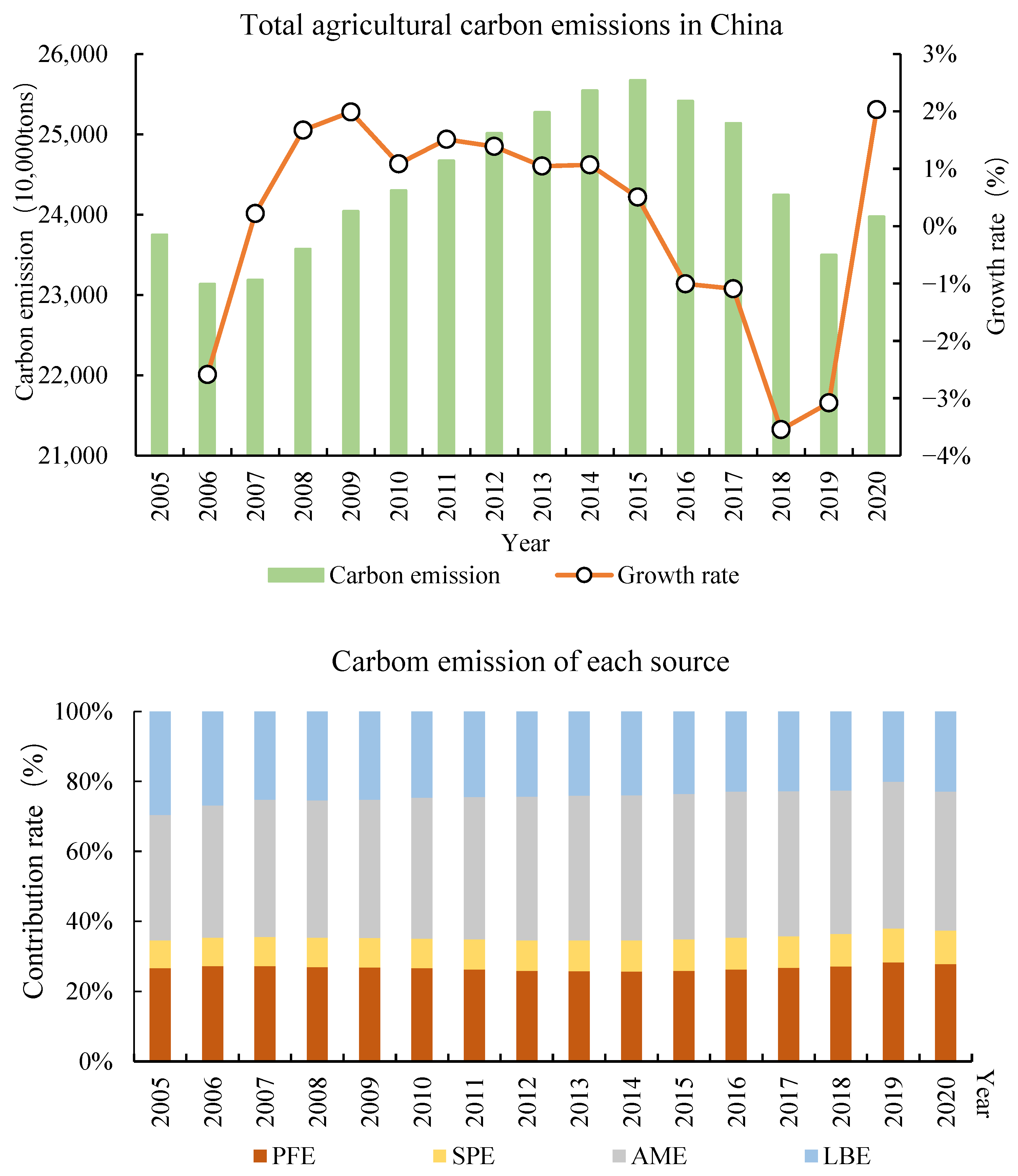
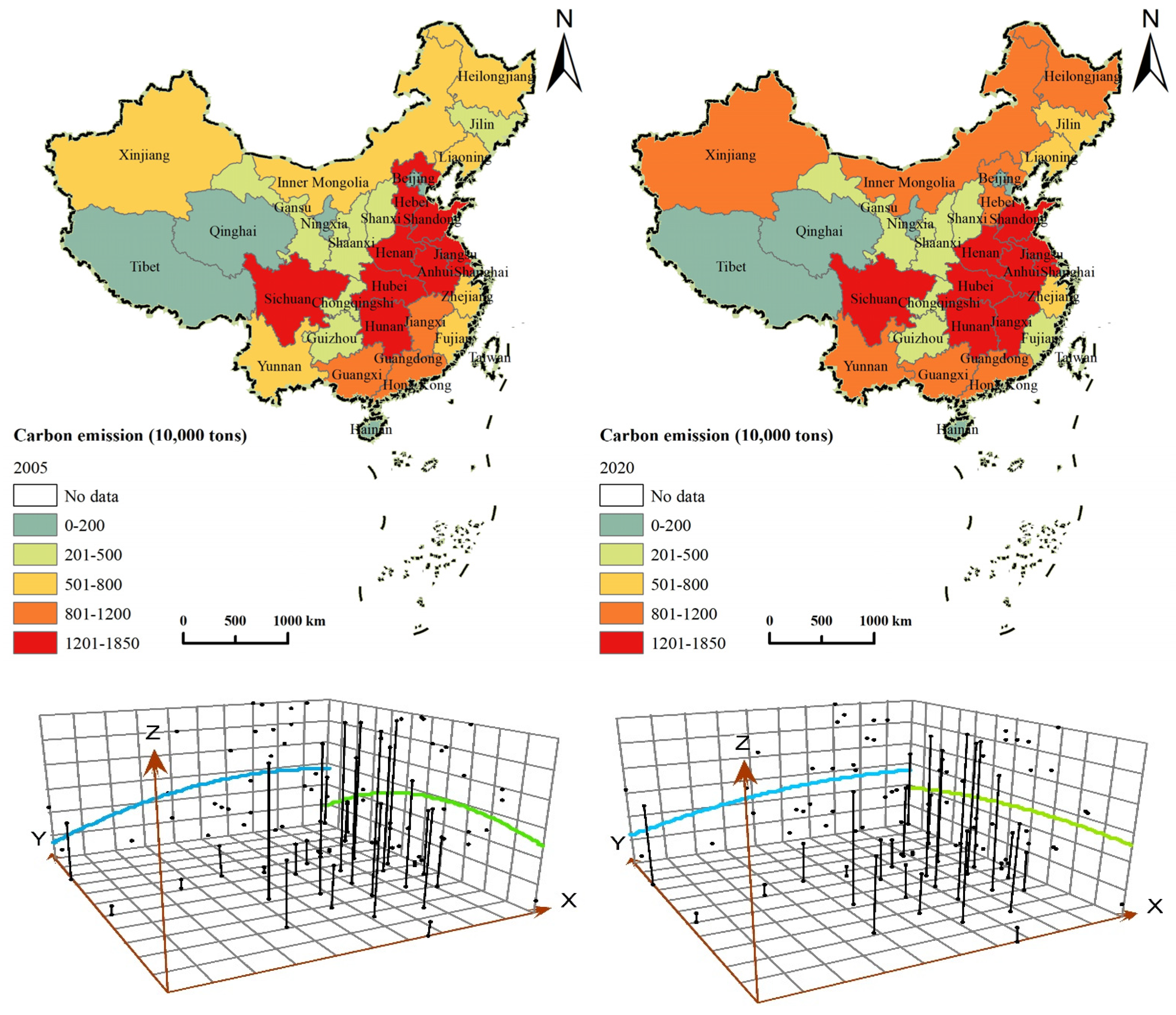
4.1.1. Regional Perspectives

As depicted in Figure 3, the overall ACE of China has undergone a dynamic shift characterized by an initial rise before decline, which is indeed consistent with Zhang et al. [58]. Specifically, it increased from 231 million tons to 257 million tons, subsequently decreasing to 235 million tons. The drivers behind this change are closely intertwined with government policies. Before 2015, the Chinese government directed its focus more towards agricultural output development and less towards ACE [59]. During the 13th Five-Year Plan period (2016–2020), the agricultural sector intensified the implementation of chemical fertilizer and pesticide usage [60], thereby curbing carbon emissions. In terms of ACE sources, AME constitutes the largest proportion, whereas SPE contributes minimally, accounting for only 9%. Regarding the contribution rate evolutionary trend, PFE, SPE, and AME exhibited an upward trajectory, while LBE decreased. Notably, in 2006, PFE surpassed AME, securing its position as the second-largest contributor to ACE.

As illustrated in Figure 4, ACE exhibits distinct imbalances. In 2005, the three provinces with the highest ACE were Hunan (17.02 million tons), Henan (16.79 million tons), and Jiangsu (16.66 million tons), whereas the three provinces with the lowest ACE were Beijing (0.62 million tons), Tianjin (0.86 million tons), and Shanghai (1.03 million tons). Interprovincial disparities primarily stem from variations in agricultural production scales. Major agricultural regions, such as Henan, Hunan and Jiangsu provinces, boast large agricultural production scales, leading to relatively high ACE. By 2020, the three provinces with the highest ACE were Hunan (18.21 million tons), Henan (16.73 million tons), and Anhui (15.91 million tons), whereas ACE in Beijing, Tianjin, and Shanghai decreased to 0.20, 0.56, and 0.76 million tons, respectively. This decline has further intensified the difference in ACE amongst various provinces.

In terms of growth rates, the provinces that witnessed the most rapid increase in ACE from 2005 to 2020 were Heilongjiang, Xinjiang, Jilin, Inner Mongolia, and Ningxia, with respective average annual growth rates of 2.87%, 2.36%, 1.9%, 1.71%, and 1.48%. Notably, these provinces are situated in the northeast and western regions. Conversely, numerous provinces experienced a decrease in ACE. Beijing, Tianjin, Hebei, Tibet, and Zhejiang showed the most significant declines, with average annual reductions of 7.2%, 2.89%, 2.62%, 2.31%, and 2.06%, respectively. Except Tibet, other provinces are located in the eastern region. Amongst the 11 provinces in the eastern region, ACE displayed a decline trend throughout the investigation period, impacting the nationwide decline in ACE. The economic improvement of the eastern region mainly depends on the tertiary industry, and the scale of agriculture continues to decline in the development process, contributing to the rapid decline in the total ACE [61].

In the trend analysis diagram, the X-axis represents the west-to-east direction, the Y-axis signifies the south-to-north direction, and the Z-axis is ACE. From the spatial distribution trends and variations, the ACE exhibited a distinct pattern of more in the east, less in the west; more in the south, less in the north. In 2005, ACE demonstrated an increasing trend along the X-axis and an inverted U-shape distribution along the Y-axis, initially ascending and subsequently descending. In 2020, ACE differences narrowed. Specifically, in the X-axis direction, the rate of upward trajectory slowed, contributing to a narrowing difference between the eastern and western regions. In the Y-axis direction, the U-shape trend considerably attenuated.

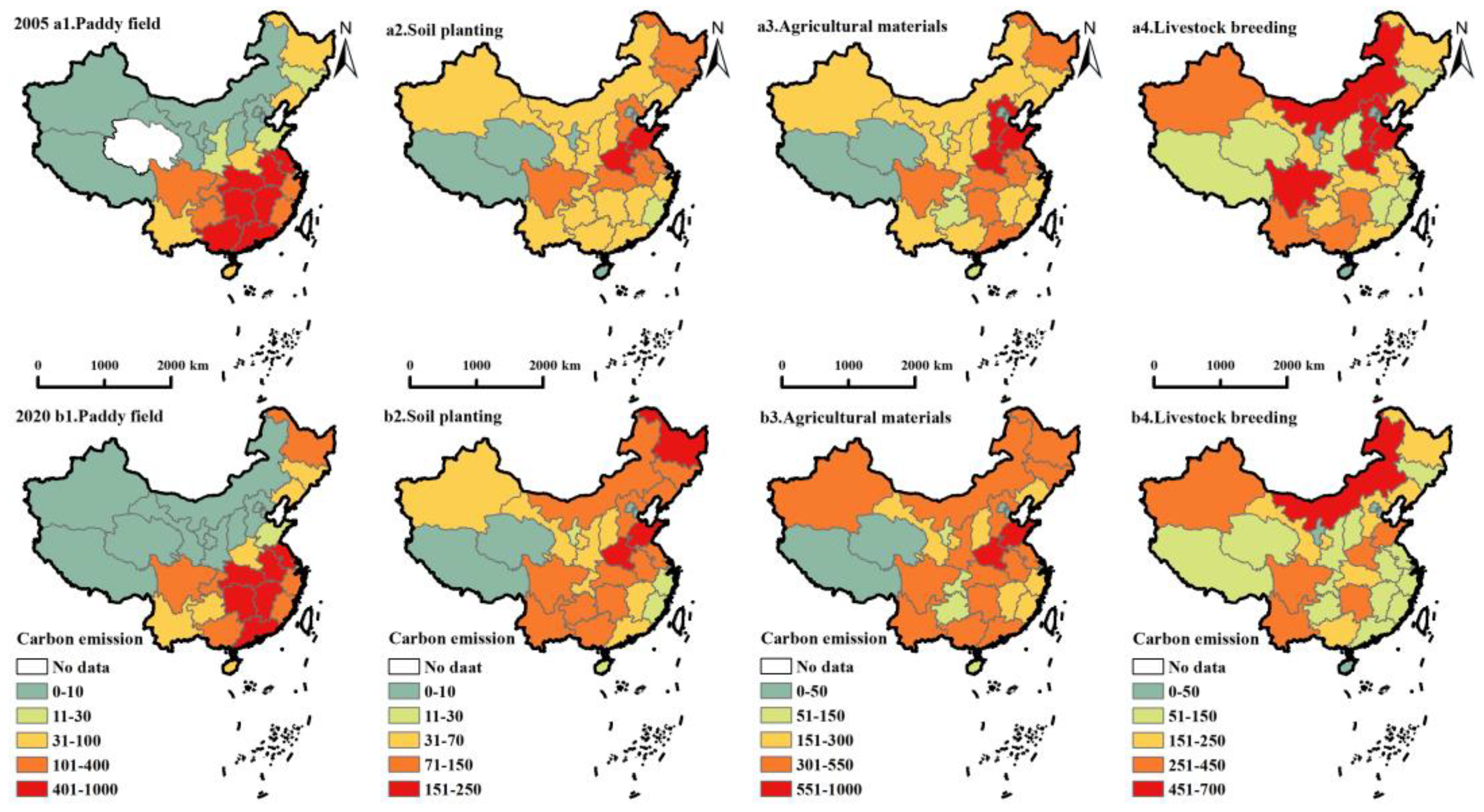
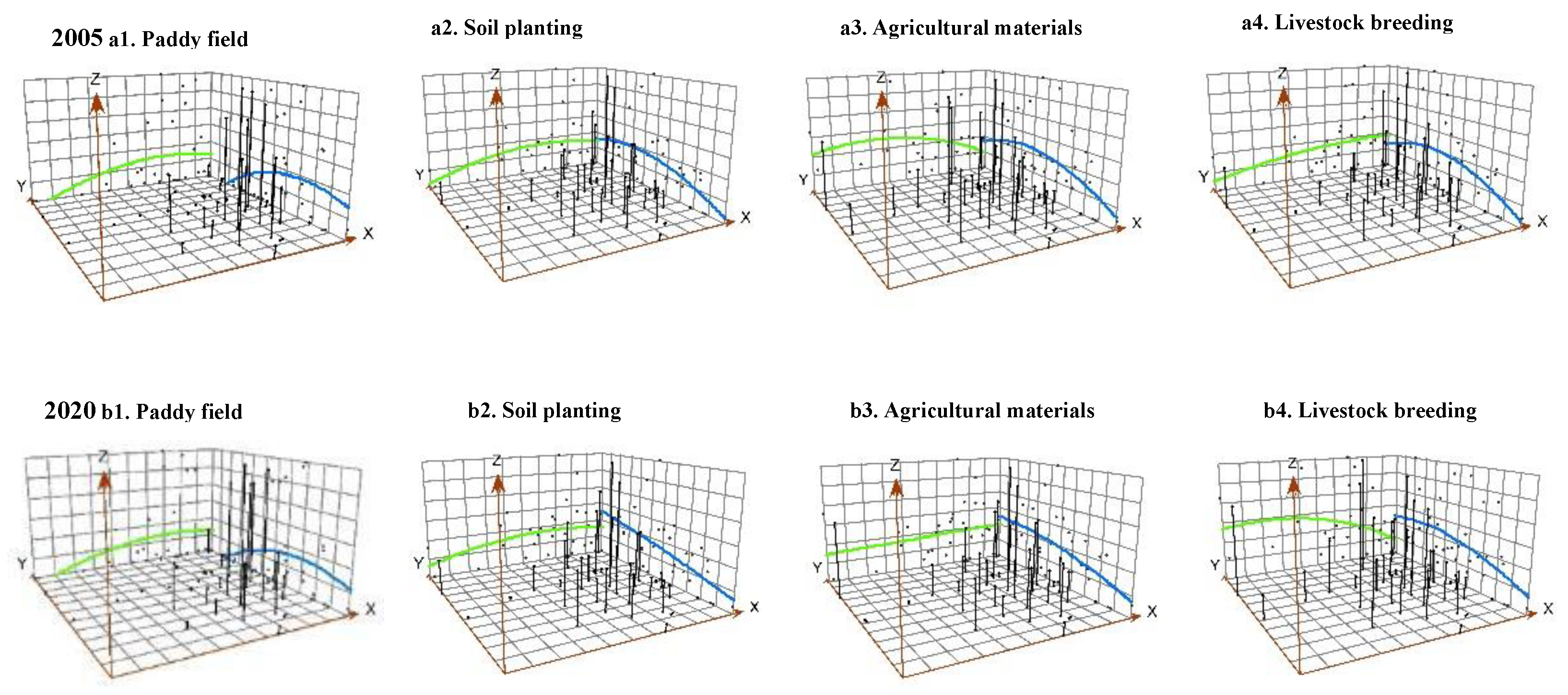
4.1.2. Carbon Source Perspectives

Distinct sources of ACE exhibit diverse spatial distributions (Figure 5), characterized by specific traits as follows. First, PFE is concentrated in the central region because the large number of paddy fields spread across the vast plains, resulting in PFE concentration [62]. Second, SPE emits less than other sources, with the highest areas observed in Henan and Shandong provinces. Third, AME is mainly concentrated in Henan and Shandong provinces. The overall AME of China in 2020 had significantly improved compared with 2005. Fourth, LBE displays notable regional differences, and the high-value area primarily concentrating in Inner Mongolia, Hebei, Shandong, Henan, and Sichuan. Over time, the LBE of most provinces has declined, with Beijing, Hebei, and Shanghai experiencing decline rates exceeding 4%.

The distribution trends and variations in ACE from different sources are illustrated in Figure 6. First, PFE displayed more in the east and less in the west in terms of regional distribution. Along the Y-axis, it exhibited an inverted U shape, initially increasing and then decreasing from north to south. By 2020, regional differences had reduced compared with 2005. Second, SPE and AME shared similar distribution characteristics. Both exhibited a pattern of more in the east, less in the west and more in the north, less in the south in terms of regional distribution. This finding contrasted with the overall ACE distribution along the Y-axis. This phenomenon was primarily caused by the northeastern region, often referred to as the ‘grain basket of China’, characterized by extensive fertile black soil. The prevailing agricultural structure in this area prioritizes cultivation, with large-scale crop farming involving substantial inputs of fertilizers and pesticides, resulting in higher SPE and AME [63]. Third, LBE followed a pattern of more in the west and less in the east, along with more in the north and less in the south in terms of regional distribution. The differences in the X-axis and Y-axis directions increased from 2005 to 2020. A large portion of LBE processes arises from the enteric fermentation and faucal management of large ruminants. In Inner Mongolia and Xinjiang province, livestock predominantly rely on natural feed. The characteristics of pasture-based farming in these regions make centralized waste management challenging, leading to higher LBE [64]. In contrast, the breeding approach in southern provinces primarily involves captive breeding, which facilitates centralized collection and emission management.

4.2. Decomposition of Spatial Differences and Sources of ACE

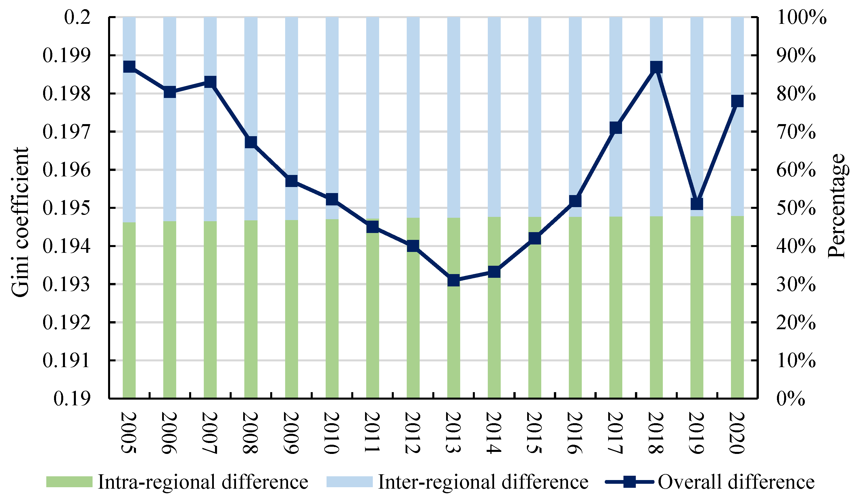
4.2.1. Overall Differences

The overall differences in ACE displayed a U-shaped trend, marked by an initial decrease followed by an increase (Figure 7). From 2005 to 2013, the overall differences in ACE exhibited a fluctuating downward trend, decreasing from 0.1987 in 2005 to 0.1931 in 2013. Subsequently, between 2014 and 2018, the overall differences in ACE underwent a rapid increase from 0.1933 in 2014 to 0.1987 in 2018. However, after 2018, the overall differences began to fluctuate. Before 2014, China’s strategy for boosting agricultural production primarily relied on increased inputs, including feed, fertilizers, and pesticides [65]. In the short term, this approach significantly boosted agricultural yields, particularly in traditional farming regions. However, it also resulted in substantial increases in agricultural pollutants and carbon emissions. Despite the reduction in regional ACE disparities during this period, total pollution and emissions continued to rise. In 2015, the Ministry of Agriculture introduced the “double reduction” policy to curb the misuse of fertilizers and pesticides, which effectively reduced carbon emissions from crop farming but had little impact on livestock-related emissions [66]. It caused an increase in the overall ACE differences. In 2020, the COVID-19 pandemic led China to impose strict restrictions on interregional movement, which also disrupted the flow of agricultural production factors. As a result, it caused fluctuations in ACE differences across regions. In terms of composition, inter-regional difference is the main source of overall difference, but its proportion is gradually decreasing, and the proportion of intra-regional difference is gradually increasing.

4.2.2. Spatial Differences from Regional Perspective

We dissect the spatial differences in ACE in China from the regional dimension (

Table 5. Decomposition of spatial differences: Four regions.

Year		2005	2007	2009	2011	2013	2015	2017	2019	2020
Gini coefficient	E-C	0.031	0.032	0.033	0.034	0.034	0.035	0.036	0.036	0.037
	E-W	0.049	0.048	0.045	0.044	0.044	0.043	0.0429	0.042	0.042
	E-N	0.011	0.011	0.010	0.010	0.010	0.010	0.0102	0.010	0.010
	C-W	0.040	0.041	0.042	0.042	0.041	0.042	0.0427	0.043	0.043
	C-N	0.010	0.009	0.010	0.009	0.009	0.009	0.0094	0.009	0.010
	W-N	0.008	0.008	0.008	0.009	0.009	0.009	0.0093	0.009	0.009
	Inter-region	0.149	0.149	0.148	0.148	0.147	0.148	0.150	0.149	0.151
	Intra-region	0.050	0.049	0.048	0.047	0.046	0.046	0.047	0.046	0.047
Contribution rate(%)	E-C	15.802	16.145	16.863	17.224	17.504	17.859	18.163	18.555	18.595
	E-W	24.811	24.218	23.199	22.776	22.527	22.131	21.766	21.425	21.425
	E-N	5.687	5.500	5.263	5.244	5.231	5.250	5.175	5.126	5.104
	C-W	20.030	20.636	21.308	21.440	21.388	21.462	21.664	21.938	21.829
	C-N	4.882	4.743	4.854	4.730	4.661	4.684	4.769	4.818	4.851
	W-N	3.825	4.137	4.241	4.473	4.661	4.735	4.718	4.716	4.699
	Inter-region	75.038	75.378	75.728	75.887	75.971	76.119	76.256	76.576	76.503
	Intra-region	24.962	24.622	24.272	24.113	24.029	23.881	23.744	23.424	23.497

and

Table 6. Decomposition of spatial differences: Two regions.

Year		2005	2007	2009	2011	2013	2015	2017	2019	2020
Coefficient	North	0.052	0.052	0.051	0.051	0.051	0.052	0.052	0.055	0.052
	South	0.040	0.041	0.040	0.041	0.041	0.041	0.0420	0.041	0.042
	Intra-region	0.092	0.092	0.092	0.092	0.092	0.093	0.094	0.093	0.095
	Inter-region	0.107	0.106	0.104	0.103	0.102	0.102	0.103	0.1020	0.103
Contribution Rate (%)	North	26.271	25.969	25.768	25.717	25.667	25.919	26.271	26.120	26.371
	South	20.030	20.483	20.332	20.483	20.483	20.634	21.087	20.785	21.288
	Intra-region	46.251	46.452	46.150	46.200	46.100	46.603	47.358	46.905	47.660
	Inter-region	53.749	53.347	52.340	51.686	51.082	51.132	51.837	51.283	51.887

) by employing bidimensional decomposition of the Gini coefficient.

Decomposing the overall differences across eastern, central, western, and northeastern regions revealed that inter-regional differences constitute the main source of ACE differences. Temporally, inter-regional differences displayed a decrease before increase, forming an overall ascending trend. The contribution ratio escalated from 75% in 2005 to 76.5% in 2020. Conversely, intra-regional differences exhibited a fluctuating downward trend, with the contribution rate decreasing from 24.96% to 23.50%. This is mainly related to the similar agricultural development structure in different regions.

To delineate the inter-regional differences in detail, we divide it into eastern–central (E-C), eastern–western (E-W), eastern–northeastern (E-N), central–western (C-W), central–northeastern (C-N), and western–northeastern (W-N) regions. In the initial period, the most substantial inter-regional differences were identified between the E-W regions, contributing to 24.8% of the overall differences. However, as time progressed, the inter-regional differences between the C-W regions becoming the primary source. The reduction in agricultural activity in the eastern region has contributed to this shift [67]. Jiangsu and Shandong provinces, characterized by flat terrain suitable for agriculture, have historically been key agricultural areas. However, the strategic advantages of their coastal locations have led to a shift in focus from primary industries to secondary and tertiary industries. From 2010 to 2020, the agricultural land area of Shandong decreased by 45%. In China’s development strategy, the central provinces of Henan and Shanxi serve as a critical line of defense for food security [68]. As a result, agricultural expansion in the central region has consistently increased, which has led to the transfer of the main sources of ACE differences between regions.

Analyzing the overall differences between northern and southern regions reveals that inter-regional differences are the major source (Table 4). Notably, the intra-regional differences increased from 0.092 to 0.095 and the inter-regional differences decreased from 0.107 to 0.103 during the sample period. This indicates that there is convergence of ACE difference between north and south. Temperature variation is the primary difference between northern and southern China [69]. For example, in the warm and humid coastal areas of the southeast, rice can be harvested three times a year, whereas in most northern regions, only two harvests are possible. Recently, global warming has led to a general temperature increase, creating favorable conditions for winter agriculture in the north. This has helped to reduce the ACE difference between regions.

4.2.3. Spatial Differences from Carbon Source Perspective

Within the framework of the Gini coefficient bidimensional decomposition method, the carbon emissions from different sources are further dissected along the carbon source dimension. This approach decomposing the spatial differences in ACE into four distinct components, PFE, SPE, AME, and LBE. The specific measurement values for this decomposition are provided as follows.

By examining the Gini coefficients for different carbon emission sources (Figure 8), we found that PFE differences play the primary role in contributing to the overall differences. Their contribution rate increased from 34.79% to 40.96% between 2005 and 2020. AME differences represent the second-largest source of overall differences, with their coefficient initially increasing and subsequently decreasing. In contrast, SPE differences exhibit an upward trend and contribute the least to the overall differences amongst the four major sources. LBE differences are characterized by a rapid decrease, with their contribution ration declining from 23.41% in 2005 to 16.21% in 2020. The analysis indicates that the spatial differences in ACE, in terms of contribution rates, originate sequentially from PFE, AME, LBE, and SPE. This is consistent with the data statistical characteristics and spatiotemporal distribution results of ACE sources.

4.2.4. Gini Coefficient Bidimensional Decomposition of Spatial Differences

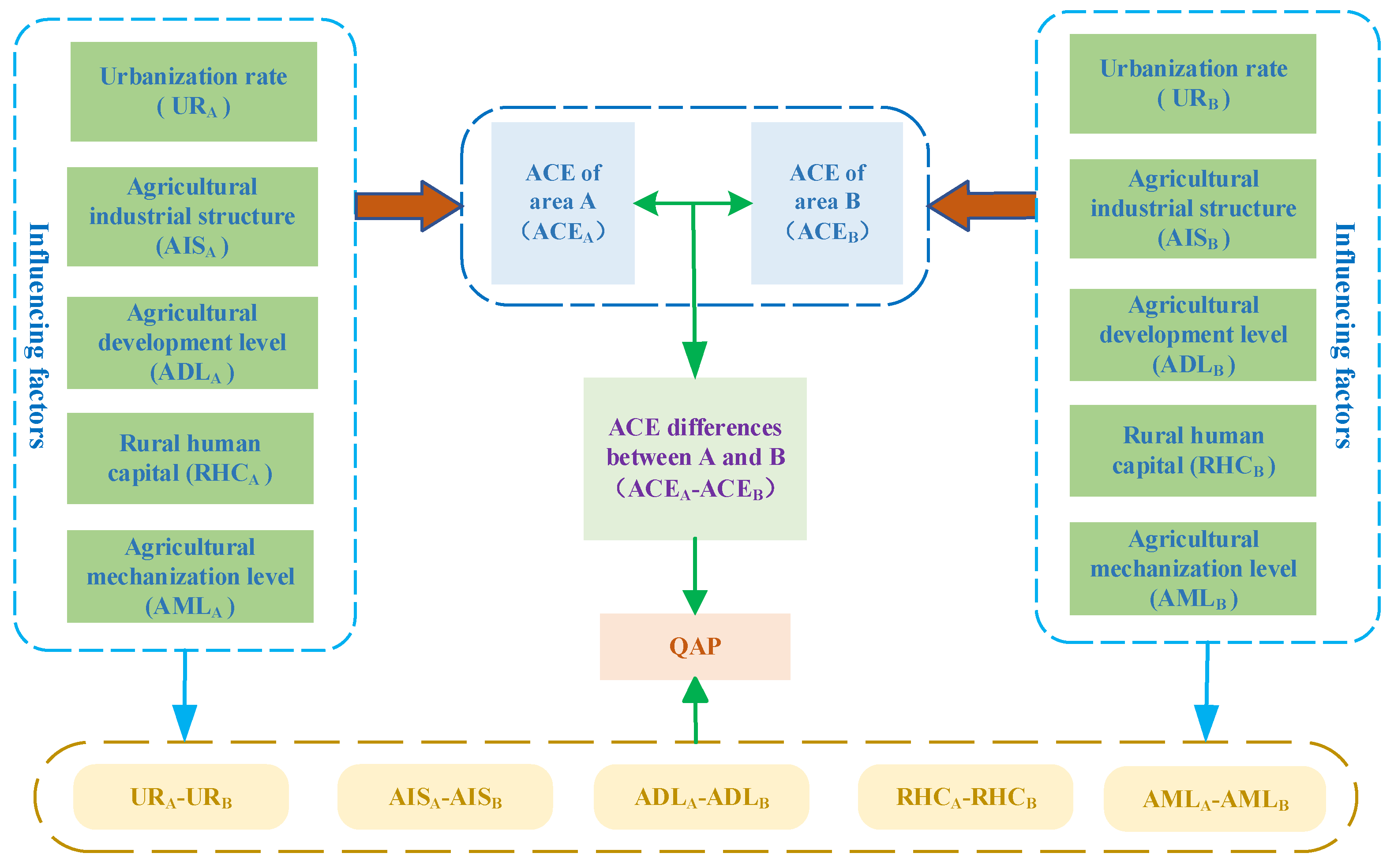
As shown in

Table 7. Gini coefficient bidimensional decomposition: Four regions.

Year	2005					2010
	PFE	SPE	AME	LBE	Total	PFE	SPE	AME	LBE	Total
E-C	5.737	1.208	4.831	4.026	15.806	7.633	1.178	5.174	3.125	17.059
E-W	6.794	1.966	10.367	5.737	24.811	5.994	1.998	10.348	4.559	22.951
E-N	1.611	0.403	2.466	1.208	5.687	1.332	0.512	2.510	0.922	5.277
C-W	10.015	1.208	5.939	2.869	20.030	11.578	1.230	6.814	1.793	21.414
C-N	2.869	0.151	1.057	0.856	4.885	3.026	0.103	1.078	0.615	4.764
W-N	1.007	0.302	1.208	1.309	3.825	1.127	0.512	1.844	0.922	4.355
Inter-region	28.032	5.234	25.818	15.954	75.038	30.635	5.536	27.715	11.937	75.820
Intra-region	6.744	1.912	8.858	7.448	24.962	6.404	2.049	9.631	6.096	24.180
Year	2015					2020
	PFE	SPE	AME	LBE	Total	PFE	SPE	AME	LBE	Total
E-C	8.651	1.184	5.046	2.987	17.868	9.955	1.162	4.649	2.830	18.595
E-W	5.304	2.163	10.093	4.583	22.142	5.609	2.173	9.146	4.497	21.425
E-N	0.978	0.772	2.523	0.978	5.252	1.112	0.707	2.426	0.859	5.104
C-W	12.204	1.236	6.334	1.648	21.473	13.643	1.213	5.761	1.213	21.829
C-N	3.141	0.052	0.927	0.566	4.686	3.335	0.101	0.809	0.556	4.851
W-N	0.978	0.721	2.163	0.875	4.737	1.061	0.657	2.173	0.809	4.699
Inter-region	31.256	6.128	27.086	11.638	76.107	34.765	5.963	24.962	10.864	76.503
Intra-region	5.870	2.214	9.938	5.922	23.893	6.215	2.324	9.601	5.356	23.497

, when decomposing from the perspective of the four major regions and carbon sources, the PFE differences between C-W regions and the AME differences between E-W regions had the largest contributions in 2005, accounting for 10.02% and 10.37% of the overall differences, respectively. However, this pattern had transformed in 2007. The PFE differences between C-W regions exceeded the AME differences between E-W regions, becoming the primary contributor to the overall differences. Moreover, their contribution rate increased over the years, reaching 13.64% in 2020. The PFE differences between E-C regions exhibited a rapid upward trend, surpassing the AME differences between E-W regions in 2020 and becoming the second source of the overall differences. Intra-regional differences played a relatively small role in the overall differences. Therefore, reducing the overall differences involves primarily focusing on narrowing the inter-regional differences in the three major regions, with a specific emphasis on addressing the differences in PFE and AME amongst these regions.

Table 8. Gini coefficient bidimensional decomposition: Two regions.

Year	2005					2010
	PFE	SPE	AME	LBE	Total	PFE	SPE	AME	LBE	Total
North	6.391	2.416	10.770	6.643	26.220	7.889	2.408	11.168	4.764	26.230
South	8.052	1.107	4.932	5.939	20.030	8.248	1.383	6.148	5.072	20.850
Intra-region	14.444	3.523	15.702	12.582	46.251	16.086	3.791	17.316	9.836	47.080
Inter-region	20.332	3.624	18.973	10.820	53.749	20.902	3.791	20.030	8.197	52.920
Year	2015					2020
	PFE	SPE	AME	LBE	Total	PFE	SPE	AME	LBE	Total
North	8.805	2.472	10.711	4.531	26.519	10.313	2.427	9.757	3.994	26.491
South	7.673	1.648	6.900	4.943	21.112	7.937	1.719	7.078	4.651	21.385
Intra-region	16.478	4.120	17.611	9.423	47.683	18.301	4.146	16.785	8.696	47.877
Inter-region	20.597	4.171	19.413	8.136	52.317	22.700	4.146	17.796	7.533	52.123

reveals that, when decomposing from the perspective of the two regions and carbon sources, the inter-regional differences in PFE emerge as the major source. Meanwhile, LBE differences exhibit intra-regional differences surpassing inter-regional ones. For other carbon sources, the distinctions manifest as inter-regional differences exceeding intra-regional ones. Throughout the period from 2015 to 2020, the inter-regional PFE differences are the main source of overall inter-regional differences, with a rising contribution rate. From the intra-regional perspective, the PFE differences in the northern region shift from the third position in 2005 to the first position in 2020 in terms of their contribution to the overall differences. In contrast, SPE differences contribute the least to the overall differences. Trends in AME differences exhibit an increase before decrease, as the contribution ratio shifts from the first to the second position in 2020. In the southern region, PFE differences play the most significant role in the overall differences, whereas SPE differences exert the least influence.

In terms of the four major regions and the north–south perspective, inter-regional differences in PFE and AME consistently emerge as the predominant sources of the overall differences. The drivers behind PFE and AME are closely intertwined with paddy cultivation, wherein the cultivated land area, quality, and irrigation methods assume pivotal roles. Notably, the distribution of cultivated land area of China follows a descending gradient of western > central > eastern regions [70]. This pattern is further exacerbated according to the second national land survey results in China, indicating a rapid reduction in cultivated land area in the east. This exacerbation intensifies the existing differences in cultivated land area amongst regions, directly amplifying the inter-regional differences in ACE [71]. Beyond that, substantial regional differences also exist in cultivated land quality and irrigation methods. The western region holds approximately 80% of low-grade cultivated land with slopes exceeding 25 degrees, which is less conducive to retaining soil and fertilizer nutrients [72]. In contrast, high-quality cultivated land is mainly concentrated in the eastern and northeastern regions. In addition, the proportion of cultivated land equipped with irrigation facilities in the eastern region significantly surpasses that in the west. Coupled with the uneven distribution of accessible irrigation water, this situation necessitates a higher input of production elements in the western region to achieve an equivalent output, subsequently leading to elevated carbon emissions [73].

4.3. QAP Analysis

4.3.1. Theoretical Frameworks

UR has both positive and negative effects on ACE. On the one hand, the rapid increase in urbanization causes the loss of agricultural land, thereby reducing ACE [74]. On the other hand, the application of new agricultural technologies in the urbanization process has improved crop yields and soil fertility mainly by increasing fertilizer use [7]. As a result, ACE is increased. Notably, the development of planting industry is usually accompanied by a large number of agricultural production factors inputting, leading to high ACE per unit of output. Therefore, an increase in the proportion of planting in AIS increases ACE [75]. ADL is one of the most direct influencing factors of ACE. When production efficiency is constant, the increase in ADL leads to a higher ACE [30]. RHC serves as an indicator of labor quality. Households with a relatively high RHC tend to possess great environmental awareness and exhibit a strong inclination towards carbon reduction during the agricultural production process [76], consequently decreasing ACE. Full-scale mechanization has become a new direction of agricultural development in China, and the use of mechanization equipment can reduce the input of human capital. However, mechanized equipment relies on fossil fuels, leading to high ACE [77].

UR, AIS, ADL, RHC, and AML exhibit significant differences amongst various regions. However, the Gini coefficient assesses regional differences from an overall perspective, which can be influenced by individual extreme values, potentially leading to inaccurate assessments of correspondence between samples. At the same time, the magnitude of the differences can only be examined from an internal source perspective, but the influence of external economic and social factors on ACE differences cannot be investigated. Conversely, the QAP analyzes the issue of regional differences by considering sample relationships between different entities. This method is better suited to exploring the factors influencing regional differences. Consequently, in the subsequent section, we use the QAP to delve further into investigating the factors that contribute to ACE differences (Figure 9).

4.3.2. QAP Relevant Analysis

QAP relevant analysis results are presented in

Table 9. QAP relevant analysis results.

Factors	Overall	Eastern Region	Central Region	Western Region	Northeast Region	Northern Region	Southern Region
UR	−0.207 *	−0.458 *	−0.168	−0.082	−0.484	−0.258	−0.158
AIS	−0.035	0.124	−0.774 **	−0.409 **	0.956	0.091	−0.410 *
ADL	0.550 ***	0.886 ***	1.476 **	0.723 *	0.891	0.740 ***	0.176
RHC	0.688 ***	0.848 ***	0.771 ***	0.588 **	0.917	0.769 ***	0.583 ***
AML	0.781 ***	0.789 ***	0.657 **	0.957 ***	0.999	0.913 ***	0.985 ***

Note: *, **, and *** indicate significance at the 10%, 5%, and 1% levels, respectively.

. At the national scale, the correlation coefficients between differences in ACE and in ADL, RHC, and AML are positive and statistically significant at the 1% level. UR demonstrates a negative correlation with ACE, reaching significance at the 10% level. From the regional perspective, the primary factors driving internal differences vary amongst regions. In the eastern and central regions, differences in ADL emerge as the foremost contributors to ACE differences. Conversely, in the western, southern, and northern regions, the influence of AML holds more prominence. All the influencing factors in the northeast region are insignificant; because there are only three provinces in northeast China, the samples are few when constructing the difference matrix. The strength of association between the dependent and explanatory variables does not necessarily equate to the extent of influence. To fully reveal the extent of each factor’s impact on ACE differences, further QAP regression analysis is required.

4.3.3. QAP Regression Analysis

The standardized regression coefficients eliminate the influence of different variable scales, enabling direct comparisons [78]. The regression coefficients and significance test outcomes of the correlation matrix variables are presented in

Table 10. QAP regression analysis results.

Factors	Overall	Eastern Region	Central Region	Western Region	Northeast Region	Northern Region	Southern Region
UR	−0.320	0.268	−0.167	−0.204	−0.009	−0.331 **	−0.209
AIS	−0.325 **	0.243 *	−0.766 **	−0.806 ***	0.808	−0.375 *	−0.419 *
ADL	0.659 ***	1.045 ***	0.944 **	1.093 **	−0.165	0.804 ***	0.249
RHC	0.290 **	0.703 ***	0.156	−0.031	0.393 ***	−0.165 **	−0.067
AML	0.584 ***	−0.231	0.651 *	0.977 ***	0.010 ***	1.058 ***	0.979 ***

Note: *, **, and *** indicate significance at the 10%, 5%, and 1% levels, respectively.

. The differences in AIS exhibit a negative correlation with ACE differences, whereas ADL, RHC, and AML display positive correlations. This implies that the narrowing of the ADL, RHC, and AML differences contributes to the mitigation of ACE differences. In contrast, the narrowing of AIS differences leads to the expansion of ACE differences. This phenomenon is primarily due to the differences in cultivation structure. The distinct provinces in China possess varying cultivation structures influenced by natural factors [79]. Different crops have different carbon emission coefficients and carbon sequestration capacities per unit output value [26]. Therefore, regional differences in cultivated structures lead to differences in ACE. Furthermore, differences in UR had no statistically significant effect on ACE differences.

The determinants of ACE differences within the eastern, central, and western regions are ADL differences. The AML differences are the primary drivers of ACE differences within the southern and northern regions, and the RHC differences are the main drivers in the northeast region. In addition, the effect of AML differences on ACE differences should be emphasized in the central and western regions. RHC differences, ADL differences, AIS differences, and AML differences are the secondary drivers of ACE differences in the eastern, southern, northern, and northeast regions, respectively.

5. Conclusions and Policy Implications

5.1. Conclusions

This study utilizes provincial-level data on PFE, SPE, AME, and LBE in China from 2005 to 2020 to compute the total ACE. Initially, the research delves into the spatiotemporal patterns of ACE variations. Subsequently, the bidimensional decomposition method of the Gini coefficient is used to dissect the specific sources. Finally, we adopt the QAP method to explore the key factors contributing to ACE differences. The primary conclusions drawn from this study are as follows.

First, between 2005 and 2020, the overall ACE of China displayed an increase before decline. The analysis result of the emissions by carbon sources shows that AME constituted the most substantial portion, whereas SPE contributed the least. In terms of spatial distribution, ACE exhibited a consistent pattern of being relatively high in the east and low in the west, as well as high in the south and low in the north. Notably, regions with elevated ACE levels were chiefly concentrated in major agricultural areas such as Henan, Hunan, and Anhui. The trend analysis indicates that ACE in most western provinces is on the rise, while ACE in eastern provinces is on the decline.

Second, the overall differences in ACE demonstrated a pattern of initial decline followed by subsequent increase. Inter-regional differences emerged as the main source of the overall differences. Conversely, differences between the northeastern region and the three other regions were relatively modest. In the context of the north–south perspective, differences between the northern and southern regions are the main source of the overall differences. The gap between inter-regional and intra-regional differences is gradually narrowing.

Third, from the bidimensional decomposition perspective encompassing the four major regions, the PFE differences between C-W regions constituted the major source of the overall differences. In the context of the bidimensional decomposition analysis focused on the northern and southern regions, the AME differences between north and south regions emerge as the key drivers of the overall differences.

Fourth, according to the QAP correlation analysis results, the overall differences in ACE demonstrated a positive correlation with the differences in ADL, RHC, and AML. Conversely, they showed a negative correlation with AIS differences. For the eastern and central regions, the differences in ADL served as the primary influencing factor for ACE differences. However, in the southern and northern regions, AML is the primary influencing factor. The QAP regression analysis outcomes revealed that differences in ADL emerge as the most prominent influence factors for ACE differences in the national sample as well as within the eastern, central, and western regions. AML differences are the main influencing factor of ACE differences within the northern and southern regions. The RHC differences are the main influencing factor in the northeast region.

5.2. Policy Implications

Several suggestions are proposed based on these research findings regarding the spatial differences and inherent structural characteristics of ACE.

First, prioritizing provinces with significant agricultural activities, such as Henan, Hunan, and Jiangsu, is crucial. This aims to unveil the inherent potential for low-carbon development within their agricultural sectors. Concurrently, the focus should be extended to the western regions, where ACE has rapidly increased. This condition entails improving irrigation, planting, and harvesting efficiency. Moreover, promoting the cultivation of superior crop varieties whilst efficiently utilizing local environmental resources can facilitate a low-carbon agricultural development strategy.

Second, addressing the inter-regional differences in PFE and AME is of paramount importance. Whether we categorize regions into the four regions or two regions, inter-regional differences consistently emerge as the predominant drivers of overall differences. When analyzing carbon sources, PFE and AME differences prominently contribute to the total differences. Therefore, a significant reduction in the overall ACE differences can be achieved by addressing inter-regional differences in PFE and AME. Moreover, fostering enhanced communication and collaboration amongst diverse regions is crucial. This approach should promote the transfer of advanced agricultural production techniques to neighboring areas.

Third, enacting differentiated ACE reduction policies adapted to local conditions and key influencing factors is recommended. ADL and AML play pivotal roles in narrowing the gap of ACE differences. On the one hand, support for agricultural innovation during the development process should be strengthened, expediting the innovation and propagation of planting and breeding modes in agriculture, animal husbandry, and fishing industries. On the other hand, an integrated urban–rural planning and industry coordination strategy should be pursued. This method involves maintaining the stability of the existing 1.8 billion mu of arable land whilst ensuring orderly agricultural development under government guidance.

5.3. Limitations

First, this study measures the ACE of China and its regional differences from provincial data given the data limitations. In the future, the study area can be further refined to provide a more precise source measurement analysis of ACE differences. In the ACE measurement, the carbon sequestration capacity of crops is not considered. In the future, the total amount of ACE and its regional differences can be further measured by considering both the carbon emission capacity and carbon absorption capacity.

Second, the Gini coefficient and QAP analysis methods used in this study have limitations in their applicability. The Gini coefficient is most effective with large sample sizes, as it requires sufficient data for accurate calculation, and the quality of the data is crucial for measuring inequality. When regional data are similar, decomposed results show minimal differences. The QAP method, requiring matrix-form data and a large sample for random permutations, may be less accurate with smaller samples or simpler networks due to limited permutations. Therefore, these methods are ideal for analyzing ACE differences in large samples, while future research should explore more appropriate methods for smaller regions.

References

1. Hough, A.M.; Derwent, R.G. Changes in the global concentration of tropospheric ozone due to human activities. Nature 1990, 344, 645–648. [Google Scholar]
2. Meinshausen, M.; Meinshausen, N.; Hare, W.; Raper, S.C.; Frieler, K.; Knutti, R.; Frame, D.J.; Allen, M.R. Greenhouse-gas emission targets for limiting global warming to 2 °C. Nature 2009, 458, 1158–1162. [Google Scholar]
3. Walther, G.; Post, E.; Convey, P.; Menzel, A.; Parmesan, C.; Beebee, T.J.; Fromentin, J.; Hoegh-Guldberg, O.; Bairlein, F. Ecological responses to recent climate change. Nature 2002, 416, 389–395. [Google Scholar] [PubMed]
4. Gilles, E.; Ortiz, M.; Cadarso, M.; Monsalve, F.; Jiang, X. Opportunities for city carbon footprint reductions through imports source shifting: The case of Bogota. Resour. Conserv. Recy 2021, 172, 105684. [Google Scholar]
5. Du, M.; Antunes, J.; Wanke, P.; Chen, Z. Ecological efficiency assessment under the construction of low-carbon city: A perspective of green technology innovation. J. Environ. Plan. Manag. 2022, 65, 1727–1752. [Google Scholar]
6. Du, M.; Zhang, J.; Hou, X. Decarbonization like China: How does green finance reform and innovation enhance carbon emission efficiency? J. Environ. Manag. 2025, 376, 124331. [Google Scholar]
7. Wang, X.; Yan, L. Driving factors and decoupling analysis of fossil fuel related-carbon dioxide emissions in China. Fuel 2022, 314, 122869. [Google Scholar] [CrossRef]
8. Ren, X.; Ni, T. National shared responsibility mechanism for carbon reduction: Addressing resource imbalances from interprovincial flows of virtual water-energy-carbon. Appl. Geogr. 2025, 177, 103576. [Google Scholar]
9. FAO. Agriculture, Forestry and Other Land Use Emissions by Sources and Removals by Sinks: 1990–2011 Analysis; FAO Statistics Division Working Paper Series; UN FAO: Rome, Italy, 2014. [Google Scholar]
10. Nayak, D.; Saetnan, E.; Cheng, K.; Wang, W.; Koslowski, F.; Cheng, Y.; Zhu, W.; Wang, J.; Liu, J.; Moran, D. Management opportunities to mitigate greenhouse gas emissions from Chinese agriculture. Agric. Ecosyst. Environ. 2015, 209, 108–124. [Google Scholar]
11. Tan, S.; Xie, D.; Ni, J.; Chen, F.; Ni, C.; Shao, J.; Zhu, D.; Wang, S.; Lei, P.; Zhao, G. Characteristics and influencing factors of chemical fertilizer and pesticide applications by farmers in hilly and mountainous areas of southwest, China. Ecol. Indic. 2022, 143, 109346. [Google Scholar]
12. Dong, H.; Liu, Y.; Zhao, Z.; Tan, X.; Managi, S. Carbon neutrality commitment for China: From vision to action. Sustain. Sci. 2022, 17, 1741–1755. [Google Scholar]
13. Li, Q.; Chen, W.; Shi, H.; Zhang, S. Assessing the environmental impact of agricultural production structure transformation—Evidence from the non-grain production of cropland in China. Environ. Impact Assess. 2024, 106, 107489. [Google Scholar]
14. Liu, M.; Yang, L. Spatial pattern of China’s agricultural carbon emission performance. Ecol. Indic. 2021, 133, 108345. [Google Scholar]
15. Kennedy, A.C.; Smith, K.L. Soil microbial diversity and the sustainability of agricultural soils. Plant Soil 1995, 170, 75–86. [Google Scholar]
16. West, T.O.; Marland, G. A synthesis of carbon sequestration, carbon emissions, and net carbon flux in agriculture: Comparing tillage practices in the United States. Agric. Ecosyst. Environ. 2002, 91, 217–232. [Google Scholar]
17. Johnson, J.M.; Franzluebbers, A.J.; Weyers, S.L.; Reicosky, D.C. Agricultural opportunities to mitigate greenhouse gas emissions. Environ. Pollut. 2007, 150, 107–124. [Google Scholar] [CrossRef]
18. Reay, D.S.; Davidson, E.A.; Smith, K.A.; Smith, P.; Melillo, J.M.; Dentener, F.; Crutzen, P.J. Global agriculture and nitrous oxide emissions. Nat. Clim. Chang. 2012, 2, 410–416. [Google Scholar]
19. Guan, N.; Liu, L.; Dong, K.; Xie, M.; Du, Y. Agricultural mechanization, large-scale operation and agricultural carbon emissions. Cogent Food. Agric. 2023, 9, 2238430. [Google Scholar]
20. Chen, Z.; Sarkar, A.; Rahman, A.; Li, X.; Xia, X. Exploring the drivers of green agricultural development (gad) in China: A spatial association network structure approaches. Land. Use Policy 2022, 112, 105827. [Google Scholar]
21. Lin, B.; Zhu, J. Impact of China’s new-type urbanization on energy intensity: A city-level analysis. Energy Econ. 2021, 99, 105292. [Google Scholar]
22. Liu, C.; Sun, W.; Li, P.; Zhang, L.; Li, M. Differential characteristics of carbon emission efficiency and coordinated emission reduction pathways under different stages of economic development: Evidence from the Yangtze River delta, China. J. Environ. Manag. 2023, 330, 117018. [Google Scholar] [CrossRef] [PubMed]
23. Zhao, R.; Liu, Y.; Tian, M.; Ding, M.; Cao, L.; Zhang, Z.; Chuai, X.; Xiao, L.; Yao, L. Impacts of water and land resources exploitation on agricultural carbon emissions: The water-land-energy-carbon nexus. Land. Use Policy 2018, 72, 480–492. [Google Scholar] [CrossRef]
24. He, Y.; Cheng, X.; Wang, F.; Cheng, Y. Spatial correlation of China’s agricultural greenhouse gas emissions: A technology spillover perspective. Nat. Hazards 2020, 104, 2561–2590. [Google Scholar] [CrossRef]
25. Zhang, X.; Xie, Y.; Jiao, J.; Zhu, W.; Guo, Z.; Cao, X.; Liu, J.; Wei, W. How to accurately assess the spatial distribution of energy CO2 emissions? Based on POI and NPP-VIIRS comparison. J. Clean. Prod. 2023, 402, 136656. [Google Scholar] [CrossRef]
26. Cui, Y.; Khan, S.U.; Deng, Y.; Zhao, M. Regional difference decomposition and its spatiotemporal dynamic evolution of Chinese agricultural carbon emission: Considering carbon sink effect. Environ. Sci. Pollut. Res. 2021, 28, 38909–38928. [Google Scholar] [CrossRef]
27. Lin, B.; Fei, R. Regional differences of CO2 emissions performance in China’s agricultural sector: A Malmquist index approach. Eur. J. Agron. 2015, 70, 33–40. [Google Scholar] [CrossRef]
28. Pan, X.; Guo, S. Decomposition analysis of regional differences in China’s carbon emissions based on socio-economic factors. Energy 2024, 303, 131932. [Google Scholar] [CrossRef]
29. Hou, M.; Cui, X.; Xie, Y.; Lu, W.; Xi, Z. Synergistic emission reduction effect of pollution and carbon in China’s agricultural sector: Regional differences, dominant factors, and their spatial-temporal heterogeneity. Environ. Impact Assess. 2024, 106, 107543. [Google Scholar] [CrossRef]
30. Han, J.; Qu, J.; Maraseni, T.N.; Xu, L.; Zeng, J.; Li, H. A critical assessment of provincial-level variation in agricultural GHG emissions in China. J. Environ. Manag. 2021, 296, 113190. [Google Scholar] [CrossRef]
31. Qin, Q.; Yan, H.; Liu, J.; Chen, X.; Ye, B. China’s agricultural GHG emission efficiency: Regional disparity and spatial dynamic evolution. Environ. Geochem. Health 2020, 44, 2863–2879. [Google Scholar] [CrossRef]
32. Cui, Y.; Khan, S.U.; Deng, Y.; Zhao, M. Spatiotemporal heterogeneity, convergence and its impact factors: Perspective of carbon emission intensity and carbon emission per capita considering carbon sink effect. Environ. Impact Assess. 2022, 92, 106699. [Google Scholar]
33. Sarkar, S.F.; Poon, J.S.; Lepage, E.; Bilecki, L.; Girard, B. Enabling a sustainable and prosperous future through science and innovation in the bioeconomy at agriculture and agri-food Canada. New Biotechnol. 2018, 40, 70–75. [Google Scholar] [CrossRef] [PubMed]
34. Zhang, L.; Pang, J.; Chen, X.; Lu, Z. Carbon emissions, energy consumption and economic growth: Evidence from the agricultural sector of China’s main grain-producing areas. Sci. Total Environ. 2019, 665, 1017–1025. [Google Scholar] [PubMed]
35. Wei, Z.; Wei, K.; Liu, J.; Zhou, Y. The relationship between agricultural and animal husbandry economic development and carbon emissions in Henan Province, the analysis of factors affecting carbon emissions, and carbon emissions prediction. Mar. Pollut. Bull. 2023, 193, 115134. [Google Scholar]
36. Han, H.; Zhong, Z.; Guo, Y.; Xi, F.; Liu, S. Coupling and decoupling effects of agricultural carbon emissions in China and their driving factors. Environ. Sci. Pollut. Res. 2018, 25, 25280–25293. [Google Scholar]
37. Su, L.; Wang, Y.; Yu, F. Analysis of regional differences and spatial spillover effects of agricultural carbon emissions in China. Heliyon 2023, 9, e16752. [Google Scholar] [CrossRef]
38. Lin, B.; Xu, B. Factors affecting CO2 emissions in China’s agriculture sector: A quantile regression. Renew. Sust. Energy Rev. 2018, 94, 15–27. [Google Scholar]
39. Tian, Y.; Zhang, J.; He, Y. Research on spatial-temporal characteristics and driving factor of agricultural carbon emissions in China. J. Intege Agric. 2014, 13, 1393–1403. [Google Scholar]
40. Huang, X.; Xu, X.; Wang, Q.; Zhang, L.; Gao, X.; Chen, L. Assessment of agricultural carbon emissions and their spatiotemporal changes in China, 1997–2016. Int. J. Env. ReS. Public Health 2019, 16, 3105. [Google Scholar]
41. Wang, G.; Liao, M.; Jiang, J. Research on agricultural carbon emissions and regional carbon emissions reduction strategies in China. Sustainability 2020, 12, 2627. [Google Scholar] [CrossRef]
42. Xiong, C.; Yang, D.; Xia, F.; Huo, J. Changes in agricultural carbon emissions and factors that influence agricultural carbon emissions based on different stages in Xinjiang, China. Sci. Rep. 2016, 6, 36912. [Google Scholar]
43. Guo, H.; Fan, B.; Pan, C. Study on mechanisms underlying changes in agricultural carbon emissions: A case in Jilin Province, China, 1998–2018. Int. J. Environ. Res. Public Heal. 2021, 18, 919. [Google Scholar]
44. Zwane, T.T.; Udimal, T.B.; Pakmoni, L. Examining the drivers of agricultural carbon emissions in Africa: An application of FMOLS and DOLS approaches. Environ. Sci. Pollut. Res. 2023, 30, 56542–56557. [Google Scholar] [CrossRef]
45. Ismael, M.; Srouji, F.; Boutabba, M.A. Agricultural technologies and carbon emissions: Evidence from Jordanian economy. Environ. Sci. Pollut. Res. 2018, 25, 10867–10877. [Google Scholar]
46. Mussard, S. The bidimensional decomposition of the gini ratio. A case study: Italy. Appl. Econ. Lett. 2004, 11, 503–505. [Google Scholar] [CrossRef]
47. Mussini, M. A matrix approach to the Gini index decomposition by subgroup and by income source. Appl. Econ. 2013, 45, 2457–2468. [Google Scholar]
48. Dagum, C. Decomposition and interpretation of Gini and the generalized entropy inequality measures. Statistica 1997, 57, 295–308. [Google Scholar]
49. Fernandes, R.; Simon, H.A. A study of how individuals solve complex and ill-structured problems. Policy Sci. 1999, 32, 225–245. [Google Scholar]
50. IPCC. Intergovernmental Panel on Climate Change (IPCC), IPCC Forth Assessment Report: Climate Change 2007 (ar4). 2007. Available online: www.Ipcc.ch-publications_and_data-publications_and_data_reports.shtml (accessed on 20 March 2025).
51. Yan, X.; Yagi, K.; Akiyama, H.; Akimoto, H. Statistical analysis of the major variables controlling methane emission from rice fields. Glob. Change Biol. 2005, 11, 1131–1141. [Google Scholar]
52. Shahbaz, M.; Loganathan, N.; Muzaffar, A.T.; Ahmed, K.; Jabran, M.A. How urbanization affects Co2 emissions in Malaysia? The application of STIRPAT model. Renew. Sustain. Energy Rev. 2016, 57, 83–93. [Google Scholar] [CrossRef]
53. Xu, B.; Lin, B. Factors affecting co2 emissions in China’s agriculture sector: Evidence from geographically weighted regression model. Energy Policy 2017, 104, 404–414. [Google Scholar] [CrossRef]
54. Dong, B.; Ma, X.; Zhang, Z.; Zhang, H.; Chen, R.; Song, Y.; Shen, M.; Xiang, R. Carbon emissions, the industrial structure and economic growth: Evidence from heterogeneous industries in China. Environ. Pollut. 2020, 262, 114322. [Google Scholar] [PubMed]
55. Yang, H.; Wang, X.; Bin, P. Agriculture carbon-emission reduction and changing factors behind agricultural eco-efficiency growth in China. J. Clean. Prod. 2022, 334, 130193. [Google Scholar]
56. Xiong, C.; Wang, G.; Xu, L. Spatial differentiation identification of influencing factors of agricultural carbon productivity at city level in Taihu lake basin, China. Sci. Total Environ. 2021, 800, 149610. [Google Scholar]
57. Dyer, J.A.; Desjardins, R.L. Carbon dioxide emissions associated with the manufacturing of tractors and farm machinery in Canada. Biosyst. Eng. 2006, 93, 107–118. [Google Scholar] [CrossRef]
58. Zhang, Y.; Yu, Z.; Zhang, J. Research on carbon emission differences decomposition and spatial heterogeneity pattern of China’s eight economic regions. Environ. Sci. Pollut. Res. 2022, 29, 29976–29992. [Google Scholar] [CrossRef] [PubMed]
59. Luo, Y.; Long, X.; Wu, C.; Zhang, J. Decoupling CO2 emissions from economic growth in agricultural sector across 30 Chinese provinces from 1997 to 2014. J. Clean. Prod. 2017, 159, 220–228. [Google Scholar] [CrossRef]
60. Jin, S.; Fang, Z. Zero growth of chemical fertilizer and pesticide use: China’s objectives, progress and challenges. J. Resour. Ecol. 2018, 9, 50–58. [Google Scholar]
61. Long, H.; Zou, J.; Liu, Y. Differentiation of rural development driven by industrialization and urbanization in eastern coastal China. Habitat. Int. 2009, 33, 454–462. [Google Scholar] [CrossRef]
62. Ahmad, S.; Li, C.; Dai, G.; Zhan, M.; Wang, J.; Pan, S.; Cao, C. Greenhouse gas emission from direct seeding paddy field under different rice tillage systems in central China. Soil Tillage Res. 2009, 106, 54–61. [Google Scholar] [CrossRef]
63. Sun, X.; Zhou, Q.; Ren, W.; Li, X.; Ren, L. Spatial and temporal distribution of acetochlor in sediments and riparian soils of the Songhua river basin in northeastern China. J. Environ. Sci. 2011, 23, 1684–1690. [Google Scholar]
64. Hu, R.; Cai, Y.; Chen, K.Z.; Huang, J. Effects of inclusive public agricultural extension service: Results from a policy reform experiment in western China. China Econ. Rev. 2012, 23, 962–974. [Google Scholar]
65. Zheng, W.; Luo, B.; Hu, X. The determinants of farmers’ fertilizers and pesticides use behavior in China: An explanation based on label effect. J. Clean. Prod. 2020, 272, 123054. [Google Scholar]
66. Du, Y.; Liu, H.; Huang, H.; Li, X. The carbon emission reduction effect of agricultural policy-Evidence from China. J. Clean. Prod. 2023, 406, 137005. [Google Scholar]
67. Xiao, W.; Zhao, G. Agricultural land and rural-urban migration in China: A new pattern. Land. Use Policy 2018, 74, 142–150. [Google Scholar]
68. Huang, J.; Yang, G. Understanding recent challenges and new food policy in China. Glob. Food Secur. 2017, 12, 119–126. [Google Scholar]
69. Yan, H.; Liu, Q.; Zhang, H.; Wang, H.; Li, H.; Yang, L. Difference in the thermal response of the occupants living in northern and southern China. Energy Build. 2019, 204, 109475. [Google Scholar]
70. Yang, H.; Li, X. Cultivated land and food supply in China. Land. Use Policy 2000, 17, 73–88. [Google Scholar]
71. Li, Y.; Li, X.; Tan, M.; Wang, X.; Xin, L. The impact of cultivated land spatial shift on food crop production in China, 1990–2010. Land Degrad. Dev. 2018, 29, 1652–1659. [Google Scholar]
72. Fang, H. Effect of soil conservation measures and slope on runoff, soil, TN, and TP losses from cultivated lands in northern China. Ecol. Indic. 2021, 126, 107677. [Google Scholar]
73. Li, X.; Jiang, W.; Duan, D. Spatio-temporal analysis of irrigation water use coefficients in China. J. Environ. Manag. 2020, 262, 110242. [Google Scholar]
74. Pandey, B.; Seto, K.C. Urbanization and agricultural land loss in India: Comparing satellite estimates with census data. J. Environ. Manag. 2015, 148, 53–66. [Google Scholar]
75. Tang, Y.; Luan, X.; Sun, J.; Zhao, J.; Yin, Y.; Wang, Y.; Sun, S. Impact assessment of climate change and human activities on GHG emissions and agricultural water use. Agric. For. Meteorol. 2021, 296, 108218. [Google Scholar]
76. Jiang, L.; Zhang, J.; Wang, H.H.; Zhang, L.; He, K. The impact of psychological factors on farmers’ intentions to reuse agricultural biomass waste for carbon emission abatement. J. Clean. Prod. 2018, 189, 797–804. [Google Scholar]
77. Wang, R.; Zhang, Y.; Zou, C. How does agricultural specialization affect carbon emissions in China? J. Clean. Prod. 2022, 370, 133463. [Google Scholar]
78. Borgatti, S.P.; Everett, M.G.; Freeman, L.C. Ucinet for windows: Software for social network analysis. Anal. Technol. 2002, 6, 12–15. [Google Scholar]
79. Li, N.; Li, Y.; Biswas, A.; Wang, J.; Dong, H.; Chen, J.; Liu, C.; Fan, X. Impact of climate change and crop management on cotton phenology based on statistical analysis in the main-cotton-planting areas of China. J. Clean. Prod. 2021, 298, 126750. [Google Scholar]
Figure 1. Regional division of study areas.
Land 14 00682 g001
Figure 2. Research framework.
Land 14 00682 g002
Figure 3. Trends and composition of ACE.
Land 14 00682 g003
Figure 4. Spatial distribution of ACE and trends in distribution.
Land 14 00682 g004
Figure 5. Spatial distribution of ACE from carbon source perspective.
Land 14 00682 g005
Figure 6. Trends in the spatial distribution of ACE from carbon source perspective.
Land 14 00682 g006
Figure 7. Overall difference composition and trend.
Land 14 00682 g007
Figure 8. Decomposition of spatial differences: Carbon sources.
Land 14 00682 g008
Figure 9. Mechanism of QAP.
Land 14 00682 g009