Article

Assessing Fine-Scale Urban Green and Blue Infrastructure Change in Manchester, UK: A Spatiotemporal Analysis Framework to Support Environmental Land Use Management

Department of Natural Sciences, Manchester Metropolitan University, Manchester M15 6BH, UK
*
Authors to whom correspondence should be addressed.
Land 2025, 14(5), 1077; https://doi.org/10.3390/land14051077
Submission received: 4 April 2025 / Revised: 2 May 2025 / Accepted: 13 May 2025 / Published: 15 May 2025
(This article belongs to the Special Issue Sustainable Urban Greenspace Planning, Design and Management)

Abstract

:
Understanding changes in urban green and blue infrastructure (UGBI) associated with land use management can inform planners on trends in environmental change that may impact urban resilience. While UGBI change resulting from land use conversion has received significant research interest, UGBI change within otherwise consistent land uses has received scant attention. This study developed a high-resolution spatiotemporal analysis framework to map fine-scale UGBI change across all land use classes in Manchester, UK, over a period (2000–2017) of significant population growth. The study found that UGBI declined in 17 out of 29 land use classes, with an overall city-wide UGBI loss of 11.9%, compared to UGBI gains for 6.4% of the city. Declines were most concerning in residential areas, which cover 33.6% of Manchester, as UGBI in these areas is important for delivering ecosystem services to citizens. Extrapolation of change rates indicate that two-thirds of future UGBI loss could occur in residential areas. These results provide insights into socio-economic processes which are likely to have similar implications for UGBI trends in other urban areas. Such knowledge is critical to inform land use planning and management to identify where UGBI is at risk and implement appropriate policies to reverse or minimise losses.

1. Introduction

Environmental features such as woodlands, street trees, rivers, ponds, wetlands, parks, shrubs, and hedges serve as a vital network of natural and semi-natural spaces, providing a wide range of recreational, cultural, and provisioning benefits to urban residents. As climate change is projected to exacerbate extreme weather events in the coming decades, this network of environmental features, or urban green–blue infrastructure (UGBI), will serve as an increasingly important resource in bolstering urban climate resilience [1,2]. Vital functions, such as stormwater absorption in canopy leaves and soils, and temperature cooling through evapotranspiration in vegetation and waterbodies regulate environmental hazards such as surface flooding and the urban heat island effect [3]. The quantification of such benefits, as ecosystem services with value to people [2], enables stakeholders to consider and contrast the relative advantages of UGBI to grey infrastructure adaptations for resident well-being [4].
Whilst many cities have adopted extensive greening programs in recent years, numerous studies suggest an overall decline in the extent and quality of UGBI in many urban centres around the world [5,6]. UGBI degradation typically occurs from infill development, whereby existing UGBI resources are replaced with impervious surfaces, or through the expansion of built infrastructure into habitats on the urban periphery [7]. As the pressure for economic development and housing continues, towns and cities become increasingly built-up, resulting in a growing population with diminishing access to ecosystem services [8].
Countering such degradation is therefore a key concern amongst many urban planning stakeholders, that benefit from the knowledge on the magnitude of UGBI change in relation to the management decisions and drivers behind it [9,10]. However, this is often difficult to measure as urban development is heterogeneous, occurring over varying spatial and temporal scales and affected by the local planning, socio-economic, infrastructure, and environmental context [11]. Complexity in urban development is typically organised through the concept of land use systems, whereby geographic extents of land are categorised according to the associated human activities and supporting land covers [12]. As a planning tool, the application of land use systems can ensure that the distribution of human activities is adequate to support economic and environmental policy goals [13].
Change in UGBI resources is therefore often approximated in land use change information, through association of an assumed proportion, configuration, or amount of UGBI per land use category [14]. For example, loss of UGBI may be assumed when converting from recreation areas, typically associated with high UGBI cover, to more built-up industrial or residential land uses. Land use therefore provides a conceptual framework to quantify structural change in an urban area and model impacts upon ecosystem services (e.g., urban cooling) and access to nature [15]. Comparison between land use, or more accurately land use land cover (LULC) map products at different time points, also provides indication of localised UGBI change according to socio-economic development pressures [14]. For example, the conversion of parkland to commercial land use may be quantified across a city, thus informing stakeholders on the environmental consequences of this change in relation to economic benefits from converting a public liability to a source of tax revenue [16].
Whilst the concept of land use is useful to investigate the effects of land conversion, consideration of UGBI change within otherwise static land use areas is also vital to understand the impacts of longer-term land management [17]. For example, numerous studies highlight increasing tendencies to convert garden UGBI (e.g., lawns, planters) to land cover types that are easier to manage and are more appropriate to support other household functions (e.g., tarmac driveways, house extensions) [18]. Land use management, described within land ownership boundaries or land use parcels [19], is often difficult to monitor due to small scales and limited planning control. Therefore, the process of UGBI removal may not be noticed by planning authorities. As demonstrated by studies of private garden land cover change, UGBI loss aggregated across numerous individual and small parcels can produce a significant overall environmental impact, such as increasing stormwater runoff rates and flood risks for the wider neighbourhood [20]. Uncontrolled loss in UGBI resources may indirectly degrade the impact of any adaptation strategy, increasing vulnerability amongst urban residents as a result.
Given recognised monitoring difficulties, UGBI changes in consistent land use parcels have received limited research attention. Since rates of land cover change can vary substantially depending on land use management [21,22], this is an important issue. For example, a study of temporal UGBI change in Berlin over a 30-year period found that greening policies in brownfields and street sides resulted in UGBI enhancement, whereas residential and parking areas suffered UGBI declines [22]. Whilst UGBI change may vary across individual land parcels, overall trends per land use can help to develop a broader understanding of the impact of specific land use pressures upon future UGBI resources and associated ecosystem services [23]. Trends considered across a wide range of land use classes can in turn aid spatial prediction of future UGBI change and therefore indicate hotspots of future UGBI decline to support the development of local UGBI strategies [24,25].
With the expansion of high-resolution digital geo-spatial data in recent years, a wide range of GIS and image analysis methods have been developed to investigate land use and land cover change in urban areas [26]. The application of advanced machine learning methods with very high resolution (<2 m pixels) multi-spectral imagery has been successfully applied to map land cover types at an appropriate patch-level scale and to improve analyses such as urban habitat connectivity modelling [27], urban heat island monitoring [28], and fine-scale land cover change detection [29]. Increasing availability of accessible datasets from public bodies and national/international mapping agencies enables consideration of broad-scale land use change [30,31], whilst also supporting finer-scale remote sensing analysis, providing ancillary data to enhance patch-level object-based land cover change comparisons [32,33].
Whilst spatial urban change analysis is an important and developing research activity, most studies focus on land cover change only or consider the concept of land use within hybrid land use land cover (LULC) categorisation systems. This study therefore attempts to address a current research gap by presenting a framework to map changes in individual UGBI patches (e.g., tree removal, grass lawn to paving) to consistent land use parcels across a city. In line with the previous discussion, this study therefore aims to develop useful urban planning information by demonstrating application of the framework to:
i.
Quantify and visualise spatial dynamics (loss and gain) in UGBI parcels at high resolution across an entire urban area.
ii.
Calculate UGBI loss/gain within each land use and extrapolate future UGBI change trends to understand risks to future urban environmental conditions.
iii.
Link vulnerability in UGBI resources (where UGBI has suffered losses) to land management practices and wider socio-economic trends.
The approach is applied to a post-industrial city (Manchester, UK) during a period of historic urban renewal and associated population growth (2000–2017). Given the similarities in socio-economic circumstances and urban configuration of Manchester to other post-industrial cities in the UK and Europe, the approach here also aims to provide comparative evidence of pan-urban trends to contribute to a growing evidence base on UGBI losses resulting from urban development.

2. Materials and Methods
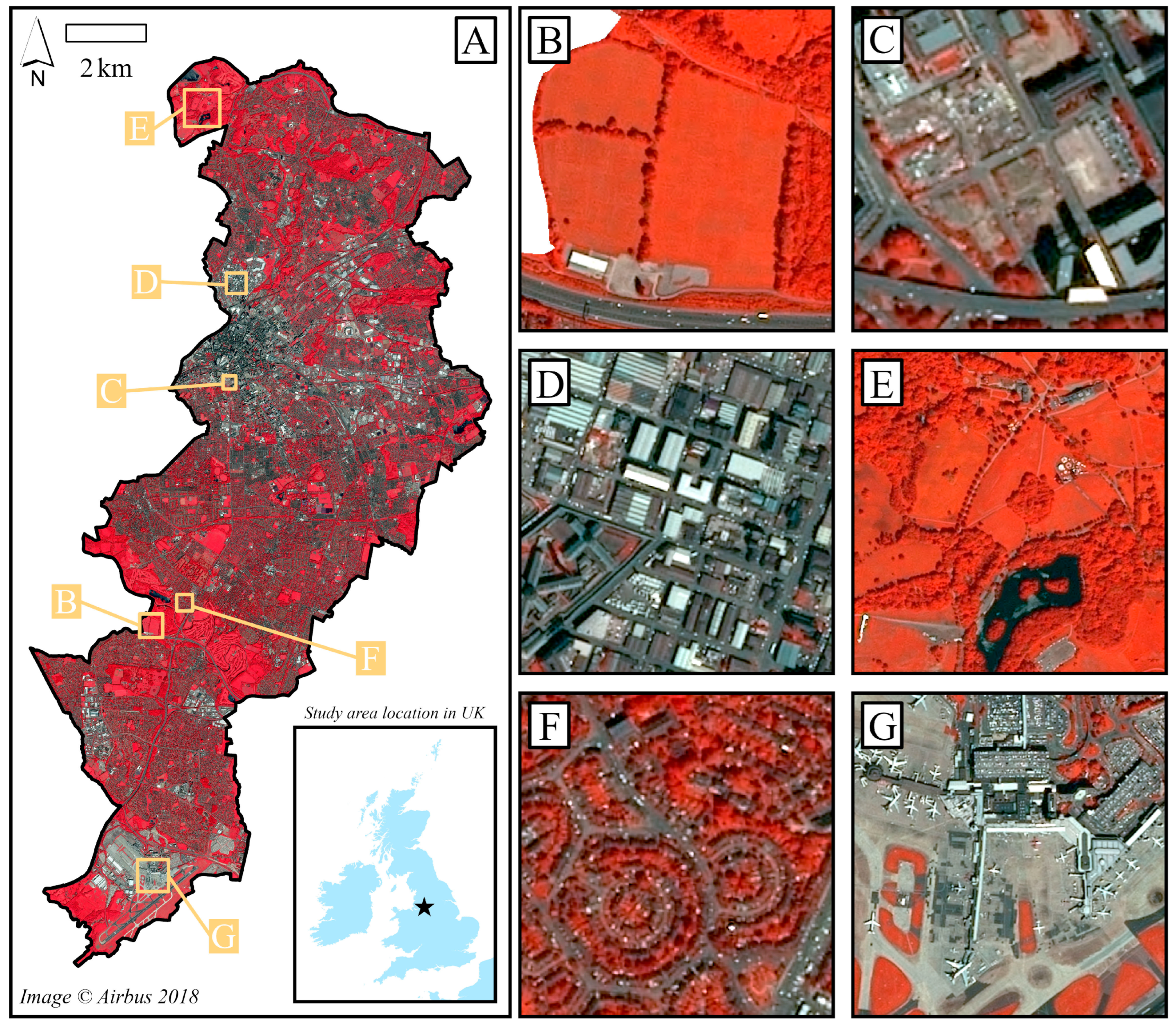
2.1. Study Area

Manchester (NW England, UK) has a population of 550,000 [34]. Patterns of land use and UGBI reflect its former industrial heritage and several phases of growth and decline since the late 1700s (Figure 1). While the city is served by a network of open (e.g., parks, nature reserves) and private (e.g., gardens) green/blue space areas, evidence suggests that UGBI cover across the city may be in decline [6]. The city population has grown rapidly since 2000 (when pop. was approximately 400,000), with many former industrial brownfield areas converted to high-density residential developments and infill development of existing UGBI patches (e.g., garden paving, building extensions). Manchester therefore provides a useful case study of UGBI change which will identify linkages between socio-economic development and land use management. Manchester City Council has recently revised its Green and Blue Infrastructure Strategy and is actively seeking to improve knowledge on UGBI to achieve climate resilience goals [35]. Furthermore, the time period of recent population growth coincides with the ready availability of very high-resolution spatial data making it suitable for GIS analysis.

2.2. Overview of Methods

The approach follows three key stages:
  • Object-based image classification, and subsequent validation, to produce a very high-resolution map of UGBI change patches.
  • Semi-automated land use mapping to identify topographic parcels and sub-parcel features that have remained consistent in land use over the study period.
  • Integration of stages (1) and (2) to identify UGBI change trends across the city, and for individual land use types, using error-adjustment methods. Visualisation of predicted future change in UGBI across the city.
Key components of the approach are summarised in the following sub-sections, with detailed notes on method processes provided in the appendices.

2.3. Mapping UGBI Change Patches

Image classification was undertaken to categorise UGBI change patches at high resolution to assess the impact of small-scale land use management processes (i.e., garden paving, re-greening of derelict buildings). For analysis purposes UGBI was defined as all identifiable vegetation features (e.g., tree canopies, grassland, planted shrubs/crops, natural shrubs) and all identifiable water features (including rivers, canals, ponds) in the imagery, irrespective of the associated land use. In this definition all sources of vegetation (green) and water (blue) serve as infrastructure, as opposed solely to explicitly planned natural resources, to provide ecosystem service benefits [37,38]. The removal of any patch of vegetation or water may have a detrimental effect on ecosystem services and local climate resilience, and therefore the same patch or water retained will continue to provide benefits as infrastructure.
Cloud-free very high-resolution (≤2 m pixel size) imagery was obtained for the years 2000 and 2017. For the year 2000, a true colour three-band (RGB) aerial image composite (0.25 m pixel size; acquired in the month of June) was purchased from commercial vendors [39]. Multi-spectral (RGB and near infrared) images were acquired from the Spot-7 (1.5 m pixel size) and Pleiades-1A (0.5 m pixel size) satellite sensors [36], respectively, for May and October 2017. Multi-date image composites are advantageous since they provide additional temporal difference information enabling enhanced vegetation classification [40]. High-resolution multi-spectral imagery was not available for the year 2000, therefore the true colour imagery was identified as the most suitable data source.
Object-based post-classification change detection was used to map UGBI change. This method compares outputs of independent classifications and is suitable for information derived from different sensors [41]. A limitation of this approach is that errors in either input classification dataset will compound within the final change detection layer [42]. A simple two-class (UGBI and non-UGBI) scheme was therefore used to generate an overall four-class (UGBI stasis, UGBI gain, UGBI loss, non-UGBI stasis) change detection map. This approach constricted error that can arise from the multiplication of unique change detection instances [43]. A rigorous manual geo-rectification process was applied to implement image co-registration to the recommended level of accuracy to minimise error from spatial mis-registration. Images were respectively cross-examined to concurrent UK Ordnance Survey MasterMapTM topographic features [44] to ensure registration of both images to a consistent spatial model. The year 2000 imagery was then downscaled to match the resolution and alignment of year 2017 image pixels to enable consistent comparison of classification outputs.
A general framework was applied to ensure similar outputs for the 2000 and 2017 land cover classification exercises. Appendix A provides a detailed overview of methods for each image date. Overall accuracy was >94% for each classified map, which enabled intersection to generate the four change detection classes (Figure 2). A separate test sample dataset was used to assess the accuracy of this output and generate final rules to clean spurious change detection patches [45], which resulted in the removal of 4.6% of the total change detection area. The final error matrix (see Appendix A) informed statistical error adjustment of change detection rates in the final stage.

2.4. Consistent Urban Land Use (ULU) Features

For the 2000–2017 study period there are no existing map products that offer consistent fine-scale land use information. Whilst the Urban Atlas [46] provides an invaluable product to analyse urban land use, the earliest version of this product is for the year 2006. Other available land use products typically amalgamate different urban land uses into a small number of categories and are more suitable for regional-scale analyses. A bespoke land use product was therefore defined, using the UK National Land Use Database (NLUD v2006; [47]) as a framework to categorise land use information from selected map layers from the UK Ordnance Survey [44]. The NLUD infers urban land use types that are recognised internationally. The urban land use (ULU) hierarchy defined in this study was based upon NLUD categories that could be feasibly identified through processing of Ordnance survey layers (see Table 1).
Mapping of study area ULU group and class categories for the year 2017 followed a semi-automated mapping approach, involving data integration, model prediction, and manual digitisation. The whole process is detailed in Appendix B and produced a vector ULU map product with a minimum mapping unit of <50 m2 (Figure 3) and overall estimated thematic accuracy of 97%. The 2017 ULU map provided a reference model to back-date consistent land use features to the year 2000.
ULU mapping at the same resolution for the year 2000 was not possible due to limitations in OS data for this period. The legacy land-line dataset for the year 2000 [48], however, maps topographic features to the same spatial model as the 2017 OS data. Polygon-to-polygon comparison between OS datasets over time enables the identification of ULU sub-parcel features that remain consistent in shape and spatial position [49], indicating consistency in underlying land use type. An automated polygon comparison algorithm was developed in R [50] to identify consistent ULU sample features (see Appendix C). The process was successful in identifying 60.2% of candidate 2017 features as samples for further analysis, which compares favourably to estimates of 76.7–85.2% for actual consistent 2017 ULU areas over the study period. UGBI change classes were clipped to each feature to aggregate UGBI change rates for ULU classes and groups.

2.5. Mapping UGBI Change

UGBI change between 2000 and 2017 was analysed for: (a) city extent, (b) individual ULU classes and class groups, (c) 100m grid cells to visualise neighbourhood trends in UGBI change (see earlier study [51] for demonstration of this grid-based approach). To account for classification error in the UGBI change detection layer, the error adjustment method described by [52] was used to estimate net UGBI change for each analysis (see Appendix D). Total error net change rates with upper (upper UGBI gain—lower UGBI loss) and lower (lower UGBI gain—upper UGBI loss) bounds of change confidence levels were calculated according to total change class composition for each analysis area. UGBI stasis was therefore determined for the respective analysis component where upper net UGBI change ≥ 0 ≥ lower net UGBI change. Net area change estimates were used to back-date estimates of UGBI levels for the year 2000. Non-stasis UGBI change trends per ULU class were used to linearly extrapolate UGBI levels approximately 17 years into the future (i.e., 2034) by applying change rates to UGBI proportions recorded for current 2017 ULU class parcels.

3. Results

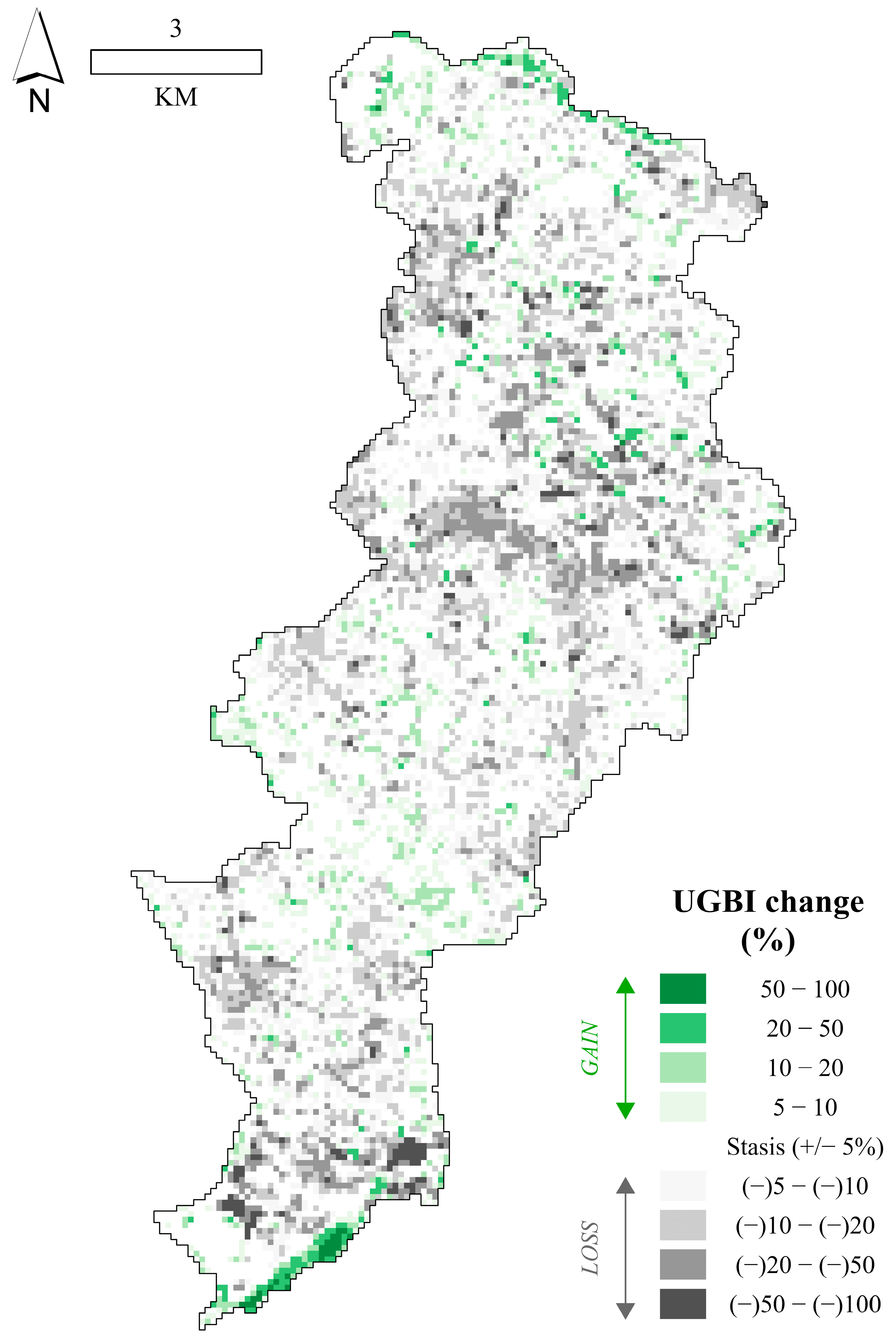
3.1. Overall UGBI Change
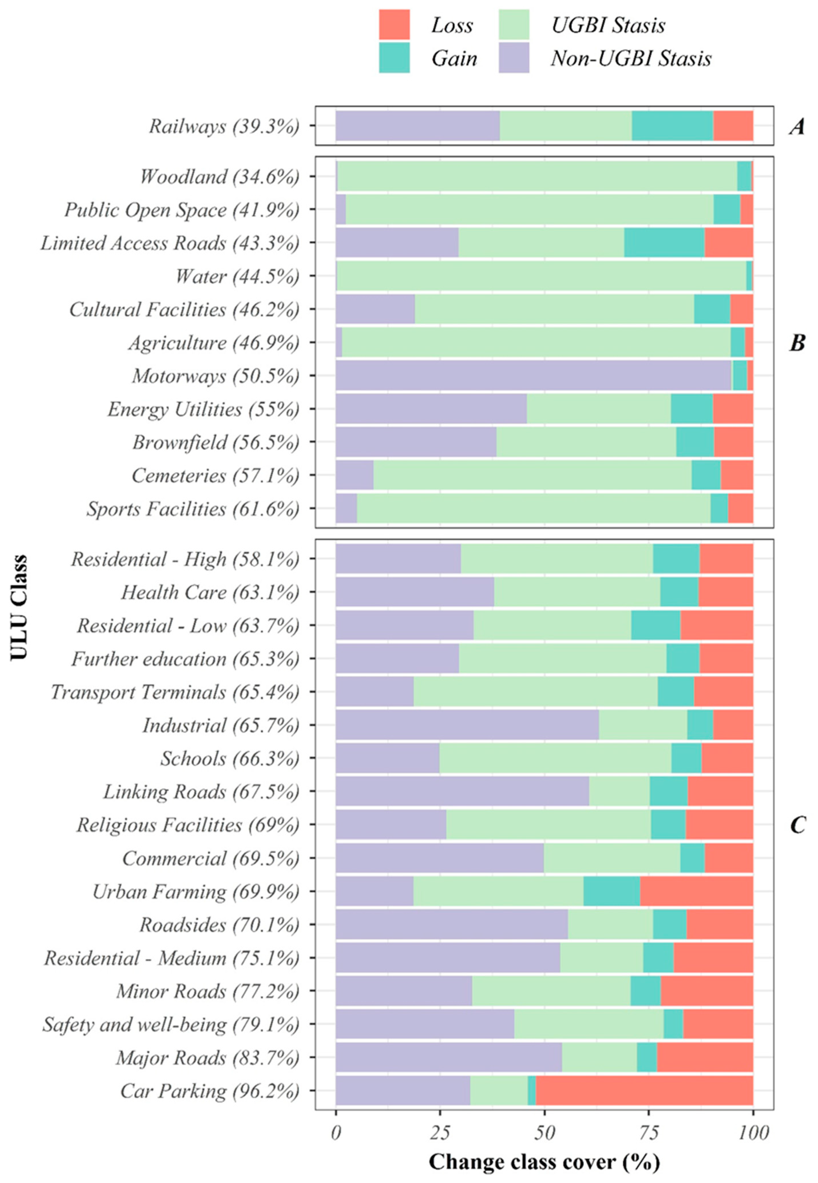
Total UGBI cover for the study area in 2000 was estimated at 50.2% (±2.6%; 95% CI), in comparison to 44.7% in 2017. This change converts to 5.5% net UGBI loss (±2.6%; 95% CI) of the total study area, or 10.9% net UGBI loss (low estimate = 6.0%, high estimate = 15.3%; 95% CI) as a percentage of the estimated UGBI in 2000. Approximate UGBI cover per resident in 2000 was 128.1 m2 compared to 99.8 m2 in 2017—a 22.1% reduction in existing UGBI per resident. However, despite the overall trend of UGBI loss, UGBI change varies across the study area. For example, 6.4% (±1.4%; 95% CI) of the study area recorded UGBI gain, in comparison to UGBI loss for 11.9% (±1.2%; 95% CI).
At the analysis cell level, net gains are recorded for 25.7% of cells in comparison to net losses recorded for 55% of cells. Figure 4 visualises this dynamism in UGBI gain and loss: existing built infrastructure has been removed and replaced with UGBI (gain), however, car-parking facilities now replace UGBI (loss). Overall, 42.7% of analysis cells showed relatively minor UGBI change (±5%; 95% CI), whilst the maximum recorded UGBI change was 77.9% and 92.2% for gain and loss cells, respectively (Figure 5). Patterns in analysis cell UGBI change exhibit a high degree of spatial autocorrelation as evidenced by the Moran’s I test (I = 0.55, p < 0.001).

3.2. Urban Land Use

Overall trends for ULU classes are largely negative; 17 out of 29 ULU classes experience statistically significant loss of UGBI (Figure 6). In comparison, Railways is the only class with net gain in UGBI, with stasis recorded for all other classes. Rates of UGBI change (as a percentage of estimated year 2000 sample UGBI cover) vary considerably between classes (Figure 7). Large losses in UGBI are apparent for Car parking (74.2%) and Major roads (41.7%). Declines in UGBI in Low-, Medium-, and High-density residential classes are 11.9%, 28.3%, and 5.7%, respectively. This indicates considerable loss in UGBI from 2000–2017 for residential areas (e.g., gardens), particularly for Medium-density residential areas characterised by terraced housing.
Change in UGBI is dynamic across ULU classes, with areas of loss and gain recorded for all classes (Figure 8). Overall UGBI change trends are determined by the balance between loss and gain UGBI cover, referred to here as the loss area dominance. Whilst the Woodland ULU class exhibits a lower loss area dominance than Railways, the overall UGBI gain trend is not significant, as the confidence intervals are neither wholly positive nor negative (Figure 5). ULU classes which have experienced overall losses in UGBI exhibit large variation in UGBI gain areas (as a percentage of total sample area) between 1.9% (Car parking) and 10.4% (Urban farming). ULU classes with stasis in UGBI exhibit ranges of 2.5–14.6% and 2.1–11.2% for gain and loss area coverage, respectively. The degree of overall UGBI change rates’ aggregate dynamism between gains and losses in UGBI thus varies between ULU classes.
Comparing overall UGBI change rates reveals similar values for a number of classes, therefore, in terms of explaining varying rates of UGBI change, some redundancy in class categorisation may be apparent. To statistically test whether differences in the distribution of estimated UGBI change rates exist, distributions of class UGBI change rates were created from exclusive random sample sub-sets. As ULU no-change sample areas vary considerably in size, thus having variable influence upon overall estimates of class UGBI change, equal size pixel groupings representing the ULU minimum mapping unit area (45 m2 = 20 pixels) were used as analysis units. The number of groups selected per class (n = 219) was determined from the number of units contained within the smallest ULU class sample pixel area (Linking roads; n = 4402 pixels/20 ≈ 219 sub-sets). UGBI change (as a percentage of existing UGBI) was then calculated for each sub-set.
As the Kruskal–Wallis test (χ2 = 2492, p < 0.001) provided strong evidence of inter-class differences in the distribution of UGBI change rates, a pairwise Wilcoxon–Mann–Whitney U test with Bonferroni correction (Base package, R Statistical Programming language; [50]) was used to test for differences between ULU classes. In all, 321 out of a total of 406 (79.1%) of class pairings displayed significant differences in estimated UGBI change rates, with the majority of non-significant differences (70 out of 85) recorded between classes of different ULU groups and the remaining non-significant differences among similar land uses within ULU groups (Appendix E). Insignificant pairings recorded for Community services (n = 5), Non-recreational open space (n = 2), and Transport (n = 8) ULU groups evidence similar development patterns and redundancy between some sub-ULU group classes. In contrast, Commercial and Industrial ULU classes represent similar land uses for private enterprise but exhibit significant differences in UGBI changes rates. Significant differences between the majority of ULU sub-group classes indicate that the current ULU class categorisation scheme provides an approximation of varying UGBI change rates within most ULU groups.

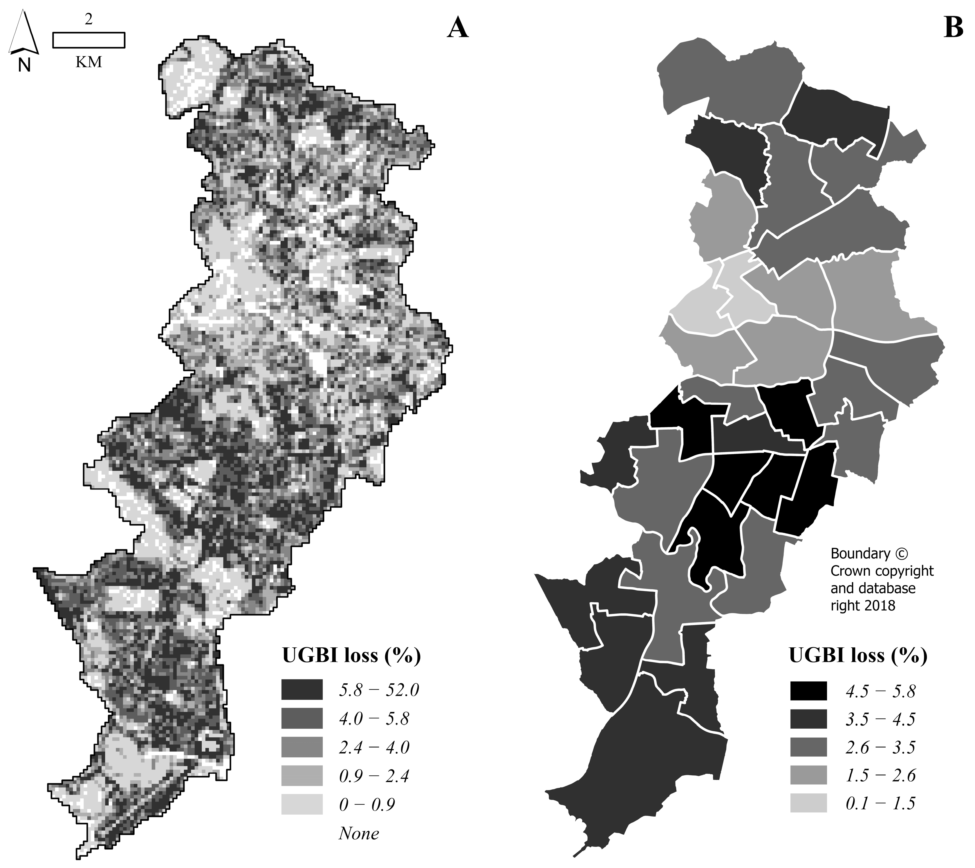
3.3. Extrapolation of Change Rates

Linear extrapolation of change rates to levels of UGBI in 2017 provides a simple method to indicate future levels of UGBI across the study area. Following this method, the majority of loss in UGBI is expected to occur within the Roadsides, Medium-density residential, and Low-density residential classes (Figure 9). Whilst rates of net UGBI change for the Low-density residential class are relatively low (−11.9%), this class contains over 20% of all 2017 UGBI. As such, assuming land use areas remain relatively static approximately 17 years into the future, current trends indicate 45% of total UGBI loss will occur within this class (Figure 9). In contrast, expected losses for Roadsides and Medium-density residential are also relatively high, with 13.5% and 19.8% total losses, respectively. All other classes record below 4% in total share of predicted loss. Relatively higher rates of UGBI loss for Car parking and the Major roads class have lower implications for future UGBI levels due to respective study area coverage of just 0.6% and 1.5% for these classes.
The implications may be examined on a spatial level at both the analysis cell and administrative ward level (Figure 10). As evidenced, high estimates of potential UGBI loss are prevalent within sub-urban residential areas south of the city centre, which contain large areas of Low-density residential areas. In contrast, when considering the study area as a whole, future UGBI cover estimates depend upon the calculation method used. When considering statistically significant UGBI change for ULU classes, UGBI cover in the 2030s is estimated to decrease by 3.1% (±1.0%; 95% C.I.). In comparison, using study area baseline change estimates for all UGBI resources, future UGBI cover is expected to decrease by a total of 4.9% (+1.9%/−2.2%; 95% C.I.). The difference between the two central estimates (1.8%) provides a basic indication of the level of UGBI change due to land use conversion. Raw neighbourhood level estimates for UGBI decline do not consider UGBI change from this process, nor additional influencing factors, and therefore currently provide an indication only of the magnitude of future UGBI decline.

4. Discussion

4.1. UGBI Change Trends

An approximate 3% decline in greenspace was measured in the city of Manchester’s urban core between 1991 and 2006 [6]. This earlier study was not representative of the city as a whole but indicates that UGBI degradation recorded here is part of an ongoing process of decline. Efforts to re-build Manchester’s post-industrial economy began in the 1980s with regeneration of the city centre and have continued apace with substantial re-development since the year 2000 [53]. Notable developments between 2000 and 2017, such as Manchester Sportcity [54] and the New Islington district close to central Manchester [55], are representative of overall economic and population growth during this period. UGBI degradation has occurred due to densification in built infrastructure [7], through land use conversion and infill development. The analysis cell (100 m) maps developed in this study therefore provide a beneficial visual guide at the neighbourhood scale where this change has occurred in the past and therefore may impact residents further in the future.
For the ULU Transport group, losses or gains in vegetation canopy will impact both Roadsides (where vegetation is likely to be planted) and adjoining road areas (where tree canopy may overhang). UGBI losses in Transport road classes are not unexpected given that countrywide urban street tree losses have been documented in the UK national press [56]. However, to the best of the authors’ knowledge, this process has not been previously quantified. Rates of UGBI decline are high for Linking, Minor, and Major roads but do not represent a significant loss of UGBI when considering total UGBI coverage within the study area. If the rates of UGBI losses in Roadsides are to remain consistent over time, then this presents a concern given that such resources are accessible to pedestrians and provide additional ecosystem services, including particulate capture and noise buffering [57].
UGBI decline recorded for Residential ULU group classes coincide with temporal declines in garden green infrastructure and pervious surface area identified in other studies [18,58,59]. For Medium-density residential areas, estimated year 2000 UGBI levels (27.3%) were already relatively low in comparison to Low-density (46.3%) and High-density (37.7%) residential classes; existing low levels of ecosystem service provision may therefore have degraded significantly further over the study period in these ULU class areas [58,60]. UGBI losses in low-density housing are less severe, but if the change rates recorded here remain consistent over time, they represent a serious concern for future ecosystem service management, given that this class covers over a fifth of the study area. Evidence from other studies indicates that population growth may influence conversion of single dwellings into multi-occupancy units, where garden paving occurs to provide car parking space for tenants [58,61]. In addition, population pressures on households may also influence decisions to extend existing housing units or sub-divide existing garden areas for new housing, in turn pressurising existing UGBI in residential areas [62,63].
The socio-economic status of home-owners may also influence management of private UGBI. For example, refs. [21,64] found differing levels of UGBI decline associated with the general affluence of districts, with higher levels of disposable income to invest in garden development. Certainly, changing lifestyles may also explain an apparent rise in “plastic lawns” in recent years, which simulate the appearance and texture of grass and are easier to manage but as a manmade surface may increase surface runoff and add unwanted plastic debris to the general environment [65]. In comparison, UGBI change rates for the High-density residential class (e.g., apartment blocks or flats) are significantly lower than those of other residential classes, as these areas are not subject to the “tyranny of small decisions” from private garden owners [66,67]. General declines in residential classes mirror UGBI declines in public (Community Services: Schools, Further education, Health care, Safety and well-being) and commercial sector (Commercial and Industrial groups) management, indicating various development pressures to do more with less land [68,69].
Whilst residential UGBI has declined, recent public surveys find that urban residents generally have positive attitudes towards urban green–blue space [70,71,72]. There is further scope in local and national policies to guide urban residents to adopt garden management practices that enhance nature conservation and climate resilience [20]. Greening efforts by environmental non-governmental organisations in Manchester [73,74] have undoubtedly contributed to the UGBI gains measured in this investigation, as evidenced by the expansion of tree canopies and tree lines (e.g., street trees, edge of woodland, or tree clusters) in many areas of the city. Indeed, a surprising finding from this investigation is the amount of dynamism between UGBI gain and loss within the study area. Net gains were recorded for Railways, whilst overall UGBI stasis was recorded for all ULU Non-recreational Open Space group classes, in addition to Public open space, and Sports facilities, indicating that consistent open space land uses over the study period witnessed limited grey development.

4.2. Limitations of the Framework and Future Research Directions

As indicated in similar remote sensing studies, change in urban landcover is typically non-linear over time [22]. Models predicting land cover change require consideration of a wide range of climatological, environmental, physical, socio-economic, demographic, and policy-level factors [30,75]. The simple extrapolation method used in this study provides a limited indication of UGBI cover into the future. To improve the analysis here, future research should take advantage of developments in accessible remote sensing imagery to repeat the process at various time points and examine the linearity of UGBI change under varying political and socio-economic conditions [76]. For example, this could be used in Manchester to examine the impact of various green strategies from the local government since 2015 [35,77] or even further into the future, consider the impacts on UGBI resources of recently adopted (February 2024) nationwide (in England) Biodiversity Net Gain legislation [78].
The information gained from this research may serve to validate the effectiveness of different UGBI protection policies and thus evidence whether direct intervention mechanisms, such as financial incentives for garden de-paving [79] or more restrictive urban planning regimes [80], could benefit conservation of UGBI and urban ecosystem services. In addition, as the GIS data used for urban land use mapping have remained consistent since 2017, the approach could be repeated to coincide with UGBI change detection exercises to consider interactions between the processes of land use and land cover development. UGBI change, resulting from conversions between distinct land use classes, could further inform research into cellular automata and machine learning approaches to improve prediction of urban environmental conditions from various development and policy scenarios [75].
Another limitation of the methodology is the use of the binary classification system that considers various vegetation and water features, with differing levels of ecosystem service benefits, as a uniform block of land cover. Whilst change detection in multiple land cover classes remains a challenge in remote sensing applications [29], future research should attempt to consider additional stratification of the UGBI class to examine changes in distinct UGBI components, such as trees, grasses, wetlands, and water, to measure change in both the quantity and quality of UGBI across the urban area [32,33]. The current framework could be used to achieve this, as incorporation of the error adjustment method enables consideration of higher rates of misclassification, which are likely to arise when incorporating additional classes into change detection processes [45]. Alternative classification approaches (e.g., direct change classification, neural networks) could also be explored as a method to ensure the retention, or even improvement of, accuracy levels in any change detection layer [29,81].
Information on the change in quality of UGBI, incorporated with improvements to the temporal resolution of land cover to land use change analysis, and improvements in change modelling, could enhance the level of projected information on future ecosystem services available to urban planning stakeholders. Given the risks posed by climate change, further research to improve methods and outcomes for UGBI change detection will become increasingly vital to support policy decisions to protect urban resident health and well-being.

5. Conclusions

This study provided a novel examination of urban green and blue infrastructure (UGBI) change within 29 urban land use classes for the case study city of Manchester, UK between the years 2000 and 2017. The main findings for Manchester include:
  • 11% of existing UGBI in 2000 was lost by 2017.
  • Dynamic change in UGBI, with 6.4% of the study area recording gains in UGBI compared to 11.9% of the study area recording losses in UGBI.
  • All urban land use classes (n = 29) record areas of UGBI gain and loss; however, overall rates, considering the balance between gains and losses, are negative for the majority (58%) of classes.
  • Projecting rates of change into the future indicates that nearly two-thirds (64%) of future UGBI loss could occur within existing Low- and Medium-density residential areas in the city.
Overall, Manchester has experienced a decline in the extent of UGBI, whilst its resident population increased in the early part of the 21st century. Local access to associated ecosystem services for the average resident over this time period is likely to have been impacted. Whilst the extrapolation methods here can only provide an indication of future UGBI provision, the overall decline in UGBI across the city is expected to persist as the population and economy of the city continue to develop (as they have done since the end of the study). This is a concern given that the ecosystem services provided by local UGBI support resident well-being and regulate the impacts of extreme weather events, which are likely to increase in severity and frequency in future with climate change.
The findings here have implications more widely across the UK and further afield in providing proxy indications of environmental change in cities that share similar socio-economic and structural characteristics. The framework offers a suitable approach adopting readily available methods and data, which may be adapted in other urban areas. To the best of our knowledge, no other study has attempted to measure this process for such a wide range of land use classes across an entire an urban area. The UGBI to land use change rates contribute novel information for further research, to improve land cover/land use change prediction, and support scenario-based policy development for effective environmental land use management.

Author Contributions

Conceptualization and methodology, F.B., G.C., G.S. and S.M.; formal analysis, F.B.; writing—original draft preparation, F.B.; writing—review and editing, G.C., G.S. and S.M.; supervision, G.C., G.S. and S.M.; project administration, G.C.; funding acquisition, G.C. and G.S. All authors have read and agreed to the published version of the manuscript.

Funding

This research was funded by Manchester Metropolitan University and UNIGIS UK.

Data Availability Statement

The datasets presented in this article have not been made publicly available due to some licensing constrictions. Requests to access the datasets should be directed to Fraser Baker (f.baker@mmu.ac.uk) who will be able to advise on a case-by-case basis.

Acknowledgments

We kindly thank the European Space Agency for supplying multi-spectral imagery for our research. We also kindly thank the independent reviewers for the time and effort for the invaluable comments regarding the manuscript.

Conflicts of Interest

The authors declare no conflicts of interest. The funders had no role in the design of the study; in the collection, analyses, or interpretation of data; in the writing of the manuscript; or in the decision to publish the results.

Appendix A

Appendix A.1. Image Classification for 2017

Appendix A.1.1. Pre-Processing

For this exercise, access to a repository of very high spatial resolution (≤5 m pixel size) multi-spectral imagery was obtained from the European Space Agency [36]. Images were acquired from the Spot-7 (1.5 m pixel size) and Pleiades-1A (0.5 m pixel size) sensors [36] for 26 May and 29 October 2017. All images were geo-referenced to the British National Grid by the vendor and pre-processed to surface reflectance. As cloud cover was evident in the October Spot-7 imagery, the affected region was replaced by October Pleiades-1A imagery downscaled to the Spot-7 resolution using nearest neighbour resampling (Raster package version 3.3-13 [82], R programming language version 3.6 [50]). Both Pleiades-1A and Spot-7 sensors share virtually identical spectral characteristics and are processed using the same radiometric correction methods [83]. In addition, both images were acquired within a thirty-minute window on the same date, therefore further pre-processing was considered unnecessary to create a composite October image.
Table A1. Sensor characteristics for Spot-7 and Pleiades-1A imagery.
SensorSpectral BandBandwidthSpatial Resolution
Spot-7 1Panchromatic0.45–0.745 μm1.5 m
Blue0.45–0.52 μm6 m
Green0.53–0.59 μm
Red0.625–0.695 μm
Near Infrared (NIR)0.76–0.89 μm
Pleiades-1A 2Panchromatic0.47–0.83 μm0.5 m
Blue0.43–0.55 μm2 m
Green0.5–0.62 μm
Red0.59–0.71 μm
Near Infrared (NIR)0.74–0.94 μm
1 ASTRIUM (October 2012). Pleiades Imagery User Guide. Retrieved from https://www.intelligence-airbusds.com/en/8289-imagery-services (accessed 5 January 2019). 2 ASTRIUM (July 2013). SPOT 6 & SPOT 7 Imagery User Guide. Retrieved from https://www.intelligence-airbusds.com/en/8289-imagery-services (accessed 5 January 2019).

Appendix A.1.2. Classification Features

Additional image feature layers were created prior to classification to enhance information in the multi-temporal image data (Table A2). Ancillary spatial data were processed using the UK Ordnance Survey (OS) MasterMap topography layer [44] to provide contextual OS landcover data for topological classification purposes (Table A3). As the datasets originate from different sources, it was important to check the degree of spatial co-registration to ensure relevant objects (e.g., buildings, roadways) in both datasets overlap the same spatial location. Root mean square spatial alignment error (tested using n = 210 random check points) [84,85] was less than one (single) pixel. Therefore, geo-rectification was not required for any input data layers.
Table A2. Image features for 2017 classification.
Image FeaturesDescriptionCalculation Method
R e d Original image layersNo processing required
G r e e n
B l u e
N I R
N D V I Normalized difference vegetation index—measure of pixel biomass photosynthetic production [86] N D V I = N I R R e d N I R + R e d
N D W I Normalized difference water index—measure of water content in water bodies [86] N D W I = G r e e n N I R G r e e n + N I R
M e a n R G B Measure of brightness of visible radiation layers—useful for determining dark pixels [87] M e a n R G B = R e d + G r e e n + B l u e 3
S d R G B Measure of pixel saturation or greyness [87] S d R G B = i = 1 n x i M e a n R G B 2 n 1
Where   n = 3 for red, green, and blue layers; x is pixel value for red, green or blue layer
R e d C H R Chromatic values for red, green, and blue layers; reduces variance in pixel illumination in image and useful for other vegetation indices [88] L y r C H R O M A T I C = L y r R e d + G r e e n + B l u e
Where   L y r represents the relevant layer for chromatic value calculation
G r e e n C H R
B l u e C H R
G R V I Green red vegetation index—measure of pixel greenness [89] G R V I = G r e e n C H R R e d C H R G r e e n C H R + R e d C H R
E X G Excess green vegetation index—measure of pixel greenness [88] E X G = 2 G r e e n C H R R e d C H R B l u e C H R
E X G E X R Excess green minus excess red index—alternative greenness index to the above [90] E X G E X R = E X G ( 1.4 R e d C H R G r e e n C H R )
P C A 1 4 x principal component layers calculated from the red, green, blue, and NIR layersCalculated using principal component function in ArcMap (version 10.5)
P C A 2
P C A 3
P C A 4
NDVIRATRatio NDVI feature between May and October images to create single index for seasonal NDVI variation N D V I R A T = o c N D V I N D V I
NDWIRATRatio NDWI feature between May and October images to create single index for seasonal NDWI variation
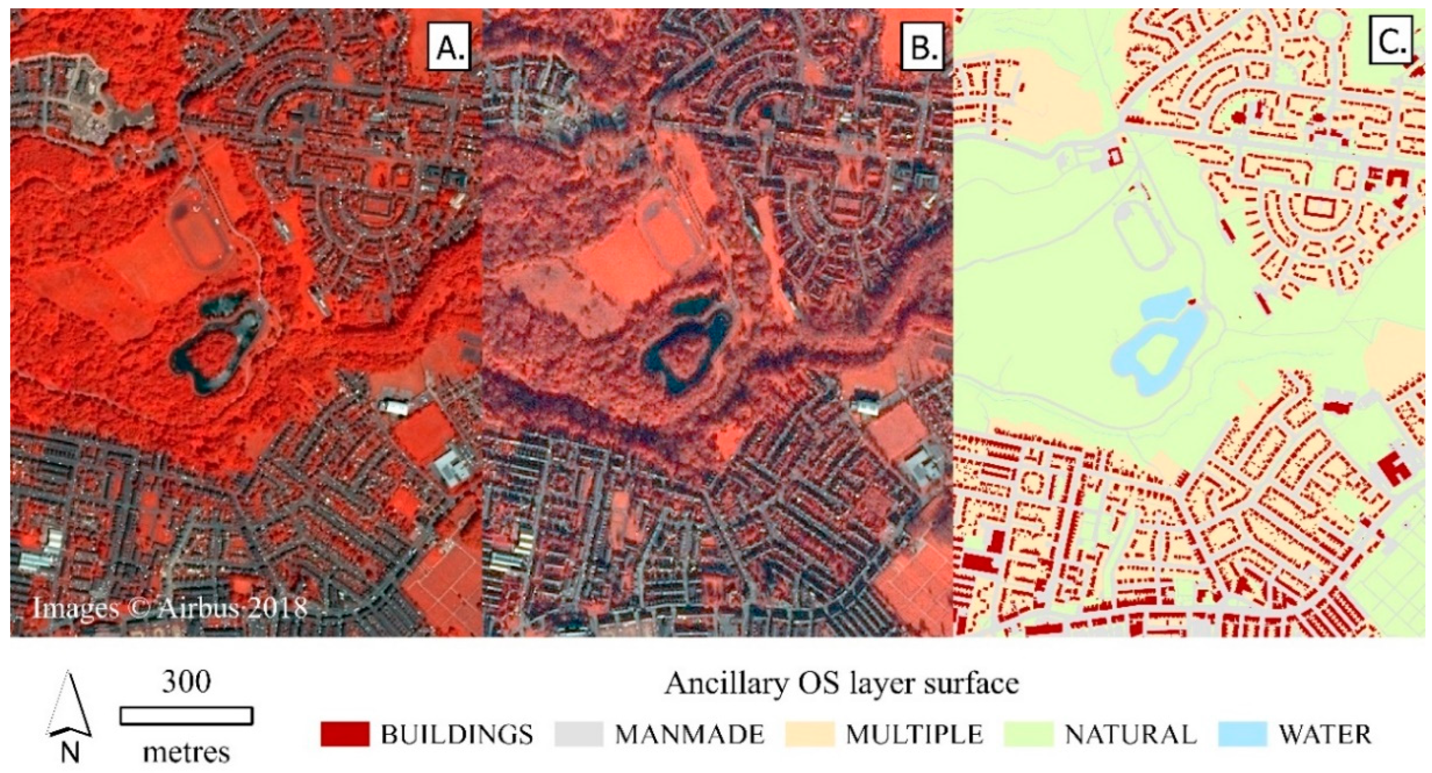
 N D W I R A T = N D V I R A T N D W I
Note: Image features were calculated for both May and October images; for May image features the layer name acronym remains the same as in the table above, for October image features the prefix oc is added to the relevant acronym. For example, Mean_RGB is referenced as ocMean_RGB when calculated for October image data only.
Table A3. Processing steps for OS ancillary dataset.
Surface Class (in Order of Processing)DescriptionClassification Ruleset (Terms in Italics Represent OSMT Attribute Field)
WATERExposed water, i.e., water channels, reservoirs, pondsdescriptiveGroup IS Inland Water, Natural Environment OR Inland Water, Structure OR Inland Water
BUILDINGSVertical standing built structuresTheme IS Buildings OR Buildings, Roads Tracks and Paths OR Buildings, Rail
NATURALNatural non-water surface such as bare earth, grass, and other vegetative surfacesMake IS Natural OR descriptiveGroup IS Landform OR Landform, Road Or Track OR Landform, Rail OR Landform, Historic Interest OR Landform, Inland Water
MANMADENon-natural surfaces, e.g., asphalt, concreteMake IS Manmade
MULTIPLEMixed NATURAL and MANMADE surfaceAll remaining records
Figure A1. Example of image and ancillary OS classification features: (A) Spot-7 May 2017 imagery (near infrared false colour) [36]; (B) Spot-7 October 2017 imagery (near infrared false colour) [36]; (C) Reclassified ancillary OS classification feature.
Land 14 01077 g0a1

Appendix A.1.3. Image Samples for Classification

Classification followed a bottom-up process whereby sub-categories of the UGBI and non-UGBI classes were first categorised using random forest models with image segmentation. The sub-categories were then processed using topological classification rules in conjunction with the OS ancillary feature dataset. A total of 2178 initial sample points were determined using multi-nomial law [91]. Multinomial law provides a method to calculate the total number of validation samples in a remote sensing classification exercise for a given number of classes (7 sub-categories here) and set confidence level (α = 0.05). The total number of initial validation samples was calculated as 726, which was then doubled to find the number of training samples based upon a 70:30 training:validation sample split [92]. This process ensured that the total number of training samples exceeded 1000 which has been found to provide a useful minimum sample number for classification in other studies [93,94] and ensured that greater than 30 samples would be available for final validation of the UGBI and non-UGBI classes [95].
Equal area reference zones (n = 33) were generated to guide the stratification of sample points across the study area with approximately 9 category samples distributed in each zone. Labels were assigned according to the sub-category class represented by the corresponding pixel in both images, and points were adjusted manually in some instances to ensure a relatively even distribution of sub-category samples across the study area. Additional points (n = 102) representing evergreen vegetation were added to the Canopy class to ensure the capture of seasonal variation in conditions in the Canopy sample (sample sizes and descriptions per sub-category are provided in Table A4). Due to difficulties in identifying the minimum number of sub-category samples in some areas of the imagery, a reduced total of 2077 samples, including 647 samples for validation, were identified following this process. Validation samples were sampled within the reference zones to ensure samples were distributed across the study area and to ensure a ≥ 30% split in the whole sample.
Table A4. Sub-category scheme and sample sizes.
Sub-CategoryDescriptionTotal No. of SamplesProportion of Total Samples (%)No. of Training SamplesNo. of Validation Samples
Artificial *Manmade non-vegetative ground surface, e.g., asphalt, concrete, paved materials28013.819783
Bare earth *Non-vegetative ground surface28413.919886
Canopy **Bole and branch canopy (shrubs/trees) vegetation38318.3261122
Grass **Ground surface herbaceous vegetation28713.719691
Water **Exposed water, i.e., water channels, reservoirs, ponds26912.818485
Shaded non-vegetation *Non-vegetation surfaces completely obscured by shadow28513.719788
Shaded vegetation **Vegetation surfaces completely obscured by shadow28913.819792
Total 20771001430647
* Non-UGBI category; ** UGBI category.

Appendix A.1.4. Classification Process

All random forest models were implemented using the random forest package in R [96] with iterative model tuning to optimise the mtry and ntree parameters. The VSURF package in R [97] was used to identify the best image features for segmentation and classification (see Table A5). Segmentation was conducted using Trimble eCognition software version 9.5.
  • Random forest classification (Initial sub-set; Table A5) to assign image pixels as either Non-Vegetation, Vegetation, Shaded non-vegetation, or Shaded vegetation.
  • Segmentation of non-vegetation pixels into objects and random forest classification (Artificial sub-set; Table A5) to assign objects as either Artificial or Bare earth.
  • Segmentation of vegetation pixels into objects and random forest classification (Canopy sub-set; Table A5) to assign objects as either Canopy or Grass.
  • All non-Canopy pixels that overlap OS ancillary water areas, re-assign to the water class.
  • All Artificial and shaded pixels that overlap OS ancillary building areas, re-assign to the Artificial class.
  • Grass and Bare earth pixels within OS ancillary manmade and building areas, re-assign to the Artificial class.
  • Manually check classified pixels against imagery for areas of misclassification and rectify.
  • Group shadow pixels into objects representing the respective shadow class and assign to respective non-vegetation or vegetation classes, according to the longest shared border to respective class objects.
  • Re-assign remaining shaded class pixels according to respective majority non-UGBI or UGBI candidate class within a 100 m circular buffer around the pixel object centroid.
  • Assign all Grass, Canopy, and Water pixels to UGBI class and Artificial and Bare earth pixels to non-UGBI class.
  • Assess accuracy using error matrix with validation samples (see Table A6).
Table A5. Segmentation and Random Forest parameters for each classification sub-set.
Sub-setInput ClassesOutput ClassesMethodSegmentation * and Classification LayersRF Settings
MtryNtree
InitialUnclassifiedNon-vegetation class, Vegetation class, Shaded vegetation, and Shaded non-vegetationPixelBlue, Red, PCA1, GreenCHR, EXGEXR350
ArtificialNon-vegetationArtificial and Bare earthObjectBlueCHR, NDWI, PCA3, RedCHR, NDVI, PCA4, SdRGB, ocNDVI, SDEV_BlueCHR, ocBlueCHR31000
CanopyVegetationGrass and Canopy (combines Deciduous and Evergreen)ObjectGreenCHR, SdRGB, BlueCHR, Red, EXGEXR, PCA3, MeanRGB, NDWI, NDVI, PCA1, PCA4, ocPCA2, SDEV_BlueCHR, Blue51000
* Segmentation (multi-resolution algorithm) parameters in eCognition (scale factor = 50, shape = 0.1 and compactness = 0.1) remained consistent for each sub-set.
Table A6. Error matrix for 2017 classification.
Non-GBIGBIUser (%)
Non-UGBI2481295.4
UGBI937897.7
Producer (%)96.596.9
Overall accuracy (%)96.8
Kappa0.93

Appendix A.2. Classification of Year 2000 Imagery

Appendix A.2.1. Pre-Processing

The year 2000 true colour aerial image (0.25 m resolution) was downscaled using nearest neighbour resampling (Raster package version 3.3-13 [82], R programming language version 3.6 [50]) to the grid resolution (1.5 m) of the 2017 classification layer. The image was then geo-referenced to within the root mean squared error (RMSE) of a single pixel, using OS land-line data from the year 2000 as a reference [98]. OS land-line data were used due to (a) < 1 pixel RMSE between 2017 OS MasterMap topography layer and year 2017 imagery, and (b) difficulty in identifying a suitable number of reference points between the year 2017 and year 2000 images. Using a spatial reference grid (n = 42 cells) as a stratification layer, reference OS land-line building polygons were randomly selected and then manually shifted to overlap the boundaries of the respective building feature in the image to create shift polygons. The centroids of original and shift polygons thus provided the reference points to calculate the appropriate rubber sheeting transformation (using ERDAS Imagine version 2019). Independent polygons for rubber sheeting translation and validation purposes [99] (approximately 30% of reference sample number) increased incrementally from 172 and 38 to 504 and 187 polygons, respectively, until <1 pixel RMSE was achieved.

Appendix A.2.2. Classification Features

Additional image feature layers were created to enhance the limited spectral information in the geo-rectified true colour imagery and thus improve the accuracy of classification (see Table A7). In addition, ancillary spatial data were processed using the year 2000 land-line data to provide contextual OS landcover data for topological classification purposes (see Table A8).
Table A7. Image feature 2000 classification.
Image FeaturesDescriptionCalculation Method
R e d Default image layersNo further processing required
G r e e n
B l u e
M e a n R G B Measure of brightness of visible radiation layers—useful for determining dark pixels [87] M e a n R G B = R e d + G r e e n + B l u e 3
S d R G B Measure of pixel saturation or greyness [87] S d R G B = i = 1 n x i M e a n R G B 2 n 1  
  where n = 3 for red, green, and blue layers; x is pixel value for red, green, or blue layer
R e d C H R Chromatic values for red, green, and blue layers; reduces variance in pixel illumination in image and useful for other vegetation indices [88] L y r C H R O M A T I C = L y r R e d + G r e e n + B l u e  
where L y r represents the relevant layer for chromatic value calculation
G r e e n C H R
B l u e C H R
G R V I Green red vegetation index—measure of pixel greenness [89] G R V I = G r e e n R e d G r e e n + R e d
E X G Excess green vegetation index—measure of pixel greenness [88] E X G = 2 G r e e n C H R R e d C H R B l u e C H R
E X R Excess green vegetation index—measure of pixel redness [88] E X G = 1.4 R e d C H R G r e e n C H R
E X G E X R Excess green minus excess red index—alternative greenness index to the above [90] E X G E X R = E X G E X R
Table A8. Ancillary OS (Land-line) classification feature.
Ancillary FeatureDescriptionMethod
BUILDINGSExtents of building features within land-line dataLand-line polygons containing land-line points representing building features *
ROADSExtents of road features within land-line dataPolygon created using a 2.5 m buffer around land-line polylines representing road centre lines
WATERExtents of water features and channels within land-line dataLand-line polygons identified with maximum shared border to land-line polyline features representing water *
* = Some manual processing required to correct misidentified features where appropriate.

Appendix A.2.3. Image Samples for Classification

Classification followed a bottom-up process whereby temporary categories were first categorised using a random forest model with image segmentation. The temporary categories were then processed using topological classification rules in conjunction with the OS land-line ancillary feature dataset. A total of 2010 initial sample points were determined using multinomial law [91]. Multinomial law provides a method to calculate the total number of validation samples in a remote sensing classification exercise for a given number of classes (initially 5 temporary categories here) and set confidence level (α = 0.05). The total number of initial validation samples was calculated as 670, which was then doubled to find the number of training samples based upon a 70:30 training:validation sample split [92]. This process ensured that the total number of training samples exceeded 1000 which has been found to provide a useful minimum sample number for classification in other studies [93,94] and ensured that greater than 30 samples would be available for final validation of the UGBI and non-UGBI classes [95].
Prior information from the 2017 classification determined the stratification of validation samples according to class coverage, which were distributed evenly across the study area using equal area reference grid zones (n = 33) as a guide. Labels were assigned according to the sub-category class represented by the corresponding pixel in both images, and points were adjusted manually in some instances to ensure a relatively even distribution of sub-category samples across the study area (sample sizes and descriptions per sub-category are provided in Table A9). Due to difficulties in identifying the minimum number of sub-category samples in some areas of the imagery, a reduced total of 1900 samples, including 670 samples for validation, were identified following this process. Validation samples were sampled within the reference zones to ensure samples were distributed across the study area and to ensure a ≥30% split in the whole sample.
Table A9. Temporary category scheme and sample sizes.
ClassTotal No. of SamplesProportion of Total Samples (%)No. of Training SamplesNo. of Validation Samples
Non-vegetation ◊69336.47462231
Shaded non-vegetation *,21011.0514070
Shaded vegetation *,ˠ24012.6316080
Vegetation ˠ70236.95468234
Water **,ˠ552.89055
Total19001001230670
* Categories merged into single shadow class for training purposes due to lack of spectral separability but retained in separate categories for UGBI and Non-UGBI validation; ** due to lack of spectral separability between water and other categories, this category was classified using topological processes only and therefore the training samples for this category were removed, the validation samples, however, were retained; ◊ Non-UGBI category; ˠ UGBI category.

Appendix A.2.4. Classification Process

All random forest models were implemented using the random forest package in R [96] with model tuning to optimise the mtry and ntree parameters. The VSURF package in R [97] was used to identify the best image features for segmentation and classification. Segmentation was conducted using Trimble eCognition software. The first step used random forest classification to assign image pixels to either the Vegetation, Non-vegetation, or shadow class, with optimal parameters: mtry = 1, ntree = 500; and classification features: Blue, Red, GreenCHR. The classified pixels were then converted to polygons to enable object-based classification with the ancillary OS (land-line) features using the rules in Table A10.
Table A10. Ruleset for object-based classification.
Candidate ClassRules for Shadow classes
Non-vegetationRelative border to Non-vegetation = 1
VegetationRelative border to Vegetation = 1
Merge all objects and intersect with WATER and BUILDINGS layer polygons
Candidate classRules for Shadow class
Non-vegetationMinimum overlap with BUILDINGS > 0
WaterMinimum overlap with WATER > 0
Non-vegetationRelative border to Non-vegetation = 1
Non-vegetationRelative border to Water AND Non-vegetation = 1
VegetationRelative border to Water AND Vegetation = 1
Merge all objects and intersect with WATER layer polygons
Candidate classRules for Non-vegetation class
WaterMinimum overlap with WATER > 0
Merge all objects
Candidate classRules for Vegetation class
Non-vegetationMinimum overlap with ROAD ≥ 0.8
Non-vegetationMinimum overlap with BUILDINGS ≥ 0.8
Re-classify non-shadow classes to either GBI or non-GBI; Segment shadow class into pixel objects
The remaining shadow pixels are re-assigned using an iterative topological process. The process iterates through individual shadow class areas in the current classification dataset by de-constructing them into pixel objects, identifying which pixel objects have non-shadow neighbours, and then iterating through the candidate pixel objects, re-classifying where appropriate to the majority neighbouring non-shadow class. If no majority class is discovered then the neighbourhood area is iteratively expanded by 1× pixel width to incorporate additional pixels until a majority non-shadow class is identified. After this stage, accuracy assessment is performed using an error matrix with the validation samples (see Table A11).
Table A11. Error matrix for 2000 GBI classification.
Non-GBIGBIUser (%)
Non-UGBI293897.3
UGBI3133891.6
Producer (%)90.497.6
Overall accuracy (%)94.2
Kappa0.93

Appendix A.3. UGBI Change Layer (2000–2017)

UGBI and non-UGBI classes for the years 2000 and 2017 were intersected to form an initial post-classification change detection layer with four change classes: UGBI loss, UGBI stasis, UGBI gain and non-UGBI stasis. Potential errors in this layer were examined in relation to both spatial misregistration and patterns of misclassification between corresponding classification layers. Object-based adjustment was implemented in a number of steps to void spurious change detection class areas [45].
First slither polygons of 1-pixel width for all change detection classes were voided from further analysis, as such areas may occur due to misregistration between the classification datasets. In addition, UGBI loss or UGBI gain classes within BUILDINGS polygons were re-classified as non-UGBI stasis. UGBI loss and gain class areas that were misclassified due to particular vegetation conditions at the time of image capture (e.g., dry canopied vegetation at the time of image collection) were examined and manually re-classified into the appropriate UGBI stasis class where identified.
Validation class sample numbers, randomly selected within stratifications according to total class area, were determined using multi-nomial law (n = 618 for 4 classes) [91]. Validation point locations were then examined in relation to both the year 2000 and year 2017 imagery to assign an appropriate change class label. Some points were voided during this process (approximately 5%) where it was difficult to ascertain the exact change class. All classes retained >30 samples for validation [95]. Validation points then populated an error matrix with the kappa statistic (see Table A12) to estimate the overall effectiveness of the change detection process.
Table A12. Error matrix UGBI change detection layer.
UGBI LossUGBI GainUGBI StasisNon-UGBI StasisUsers (%)
UGBI loss6004192.3
UGBI gain0358277.8
UGBI stasis43209196.3
Non-UGBI stasis62025196.9
Producers (%)85.787.594.698.4
Overall accuracy (%)94.7 Kappa0.92

Appendix B

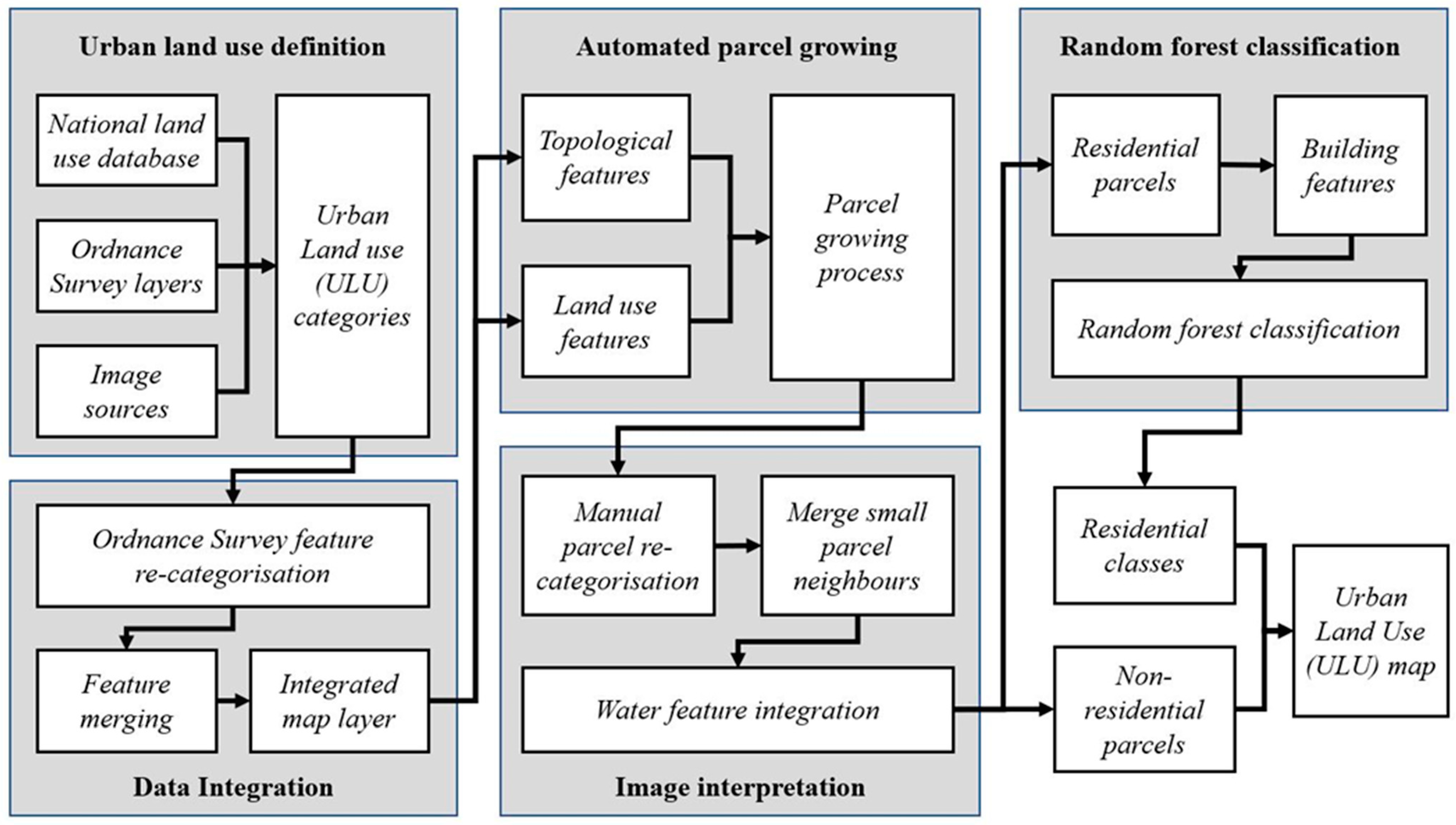
Appendix B.1. Method Overview

Methods were developed to maximise the information from all available layers to map urban land use (ULU) efficiently and accurately across the study area (see Figure A2). The main stages are as follows:
  • ULU categories were defined using the UK NLUD [47] as a framework (see main article, Section 2.4).
  • Integration of existing data in Ordnance Survey data layers (Table A13) to directly categorise urban land use (ULU) for as much of the study area as possible.
  • Automated parcel growing after initial ULU categorisation to group remaining non-assigned topographic features (such as buildings, access paths, and general enclosures) into parcels that adequately represent a single land use [100].
  • Assignment of ULU labels to non-assigned parcels through manual image interpretation in conjunction with the Spot-7 and Google Earth imagery.
  • Random forest classification to classify initial ULU residential group areas into either Low-, Medium-, or High-density residential ULU classes.
  • Validation of final ULU map dataset.
Table A13. Ordnance Survey (OS) data layers required for urban land use categorisation.
Product *VersionDescription
MasterMap Sites LayerOctober 2017Spatial extents of important locations such as airports, schools, hospitals, utility and infrastructure sites
MasterMap Greenspace LayerJuly 2017Spatial extents of publicly accessible and non-accessible greenspace areas within urban areas
MasterMap Topography LayerMay 2017Detailed spatial data representing physical (e.g., surface extents, physical boundaries, buildings, paths) and non-physical (e.g., administrative and electoral boundaries, cartographic text, symbols) features
Open Map Local (Vector)October 2017Open access street-level mapping vector data product containing additional extents of useful urban sites not defined within the above layers
MasterMap Highways NetworkOctober 2017Route lines for highways (roads and paths) network for geo-spatial network analysis
Building Heights (Alpha)October 2017Consisting of a number of different height attributes for each building in the MasterMap Topography Layer
* = all Ordnance Survey products licenced from Edina Digimap AC0000851941 (see https://digimap.edina.ac.uk/ accessed on 9 December 2019); technical information for each layer (see www.ordnancesurvey.co.uk; accessed on 18 January 2020).
Figure A2. Method workflow to map the Urban land use (ULU) data layer.
Land 14 01077 g0a2

Appendix B.2. Urban Land Use (ULU) Definition

Relationships between the National Land Use database (version 2006) and urban land use (ULU) 2017 classification, varying from one ULU class to one NLUD class, one ULU class to many NLUD groups, or many ULU classes to one NLUD group, were found. Mapping methods trialled with OS data layers indicated achievable levels in ULU thematic resolution relative to existing UK NLUD categories.
Table A14. Relationships between NLUD 2006 and ULU.
NLUD 2006ULU 2017
ORDERGROUPCLASSGROUP
AGRICULTURE & FISHERIESAgriculture5.1 AgricultureNon-recreational Open Space
Fisheries
FORESTRYManaged forest5.4 Woodland
Un-managed forest
MINERALSMineral workings & quarriesNot identifiableNot identifiable
RECREATION & LEISUREOutdoor amenity & open spaces6.1 Public open spacePublic Recreation
Amusement & show placesNot identifiableNot identifiable
Libraries, museums & galleries3.2 Cultural facilitiesCommunity Services
Sports Facilities & grounds6.2 Sports facilitiesPublic Recreation
Holiday parks & camps7.1 Low-density residentialResidential
Allotments & city farms6.3 Urban farmingPublic Recreation
TRANSPORTTransport tracks & ways8.6 MotorwaysTransport
8.4 Major roads
8.3 Linking roads
8.5 Minor roads
8.2 Limited access roads
8.8 Roadsides
8.7 Railways
Transport terminals & interchanges8.9 Transport terminals
Car parks8.1 Car parking
Other Vehicle storage
Goods & freight handling4.1 IndustrialIndustrial
Waterways5.3 WaterNon-recreational Open Space
NLUD 2006ULU 2017
ORDERGROUPCLASSGROUP
UTILITIES & INFRASTRUCTUREEnergy production & distribution4.2 Energy utilitiesIndustrial
Water storage & treatment5.3 WaterNon-recreational Open Space
Refuse disposal4.1 IndustrialIndustrial
Cemeteries & crematoria5.2 CemeteriesNon-recreational Open Space
Post & telecommunications2.1 Commercial
Commercial
RESIDENTIALDwellings7.1 Low-density residentialResidential
Dwellings7.2 Medium-density residential
Dwellings7.3 High-density residential
Hotels, boarding & guest houses
Residential institutions
COMMUNITY SERVICESMedical & health care services3.3 Health careCommunity Services
Places of worship3.5 Religious facilities
Education3.6 Schools
Education3.4 Higher education
Community services3.1 Safety and well-being
RETAILShops2.1 CommercialCommercial
Shops
Financial & professional services
Restaurants & cafes
Public houses, bars & nightclubs
INDUSTRY & BUSINESSManufacturing4.1 IndustrialIndustrial
Offices2.1 CommercialCommercial
Storage4.1 IndustrialIndustrial
Wholesale distribution
VACANT & DERELICTVacant1.1 BrownfieldBrownfield
Derelict
DEFENCEDefenceSafety and well-beingCommunity Services
UNUSED LANDUnused land1.1 BrownfieldBrownfield

Appendix B.3. Process Steps to Create the Urban Land Use (ULU) Layer

The steps listed below (Table A15) relate to the various stages of the method overview diagram (Appendix B.1). Steps 1–11 relate to the hierarchical integration of OS data to produce the initial ULU class and group areas. Steps 12–15 relate to automated parcel growing routine. Steps 16–20 relate to manual image interpretation. Steps 21–23 relate to random forest classification of residential ULU areas and final rectification of the ULU layer.
Table A15. Step by step process to create the Urban land use (ULU) layer.
StepDescription
1Select and extract OS MasterMap Topography Layer (OSMT): Polyline features representing obstructing features to create Obstructing polylines data. Obstructing polylines represent above-ground features such as fences, walls, hedges etc. that prevent pedestrian access to enclosed areas. Obstructing polylines represent features that define distinct land parcel areas within the OS Topography dataset.
2Intersect Obstructing polylines with study area boundary to create set of polygon areas (BASE OS) with unique ID reference and all with MERGE label pOSMT.
3Re-classify OSMT: Polygons with MERGE labels where the following attribute conditions are met:
MERGE label *THEME containsTHEME excludesDESCRIPTION contains
pBUILDINGSBuildingsRail OR Roads Tracks and Paths OR Watern.a.
pPATHRoads Tracks And PathsRail OR WaterPath
pROADRoads Tracks And PathsRail OR WaterRoad Or Track
pWATERWaterRail OR Roads Tracks and Pathsn.a.
RailwaysRailn.a.n.a.
RoadsidesRoads Tracks And PathsRail OR WaterRoadside
* Labels beginning with a lower case p represent preliminary class polygons to be categorised into final ULU classes in subsequent steps. Other labels represent final ULU classes. Extract re-class label polygons only from the OSMT: Polygons data to create PRLM ULU.
4Erase BASE OS polygons using the extents of PRLM ULU, and then merge to form PRLM OS dataset.
5Re-classify OS Open Map local (OPMP: Important building points) points with MERGE labels where the following conditions are met:
MERGE labelCLASSIFICATION contains
Community servicesFire station OR Police station
Cultural facilitiesArt Gallery OR Library OR Museum OR Tourist information
Health careHospice OR Hospital OR Medical care accommodation
Higher educationFurther education OR Higher or university education
Religious facilitiesPlace of worship
SchoolsNon-state primary education OR Non-state secondary education OR Primary education OR Secondary education OR Special needs education
Sports facilitiesSports and leisure centre
Transport terminalsAirport OR Bus station OR Coach station
6Re-classify PRLM OS buildings containing re-classified OPMP building points with appropriate MERGE label.
7Re-classify Highways—All: MasterMap Highways Network (NTWK) polylines where the following conditions are met:
MERGE labelrouteHierarchy attributes
MotorwaysMotorway
Major roadsA road primary, A road
Linking roadsB road, B road primary
Minor roadsMinor road, Local road, Local access road
Limited access roadsRestricted local access road, Restricted secondary access road, Secondary access road
8Re-classify PRLM OS pROADs polygons with MERGE label from contained NTWK polyline.
9Re-classify OS MasterMap Sites Layer (SITES) polygons where the following conditions are met:
MERGE labelSite Layer attribute: Function
Energy utilitiesGas Distribution or Storage OR Electricity distribution
Health careHospice OR Hospital OR Medical care accommodation
Higher educationFurther education OR Further education, Higher or university education OR Higher or university education
RailwaysRailway station
SchoolsFurther education, Non-state primary education OR Further education, Non-state secondary education OR Further education, Secondary education OR Non-state primary education OR Non-state primary education, Non-state secondary education OR Primary education OR Primary education, secondary education OR Secondary education OR Special needs education OR Non-state secondary education
Transport terminalsAirport or Bus station or Coach station
10Re-classify and retain OS MasterMap Greenspace (GRNS) layer polygons where the following conditions are met:
MERGE labelGreenspace Layer: Primary Function (priFunc)
BrownfieldNon-functioning
CemeteriesCemetery
Public open spacePublic park Or Garden
Religious facilitiesReligious grounds
ResidentialCamping Or Caravan park OR Private gardens
Sports facilitiesBowling green OR Golf course OR Play space OR Playing field OR Tennis court OR Other sports facility OR Formal recreation
Urban farmingAllotments or community growing spaces
11Erase GRNS polygons using SITES polygons and then erase PRLM OS using GRNS and SITES layers in turn. Merge GRNS, SITES, and PRLM OS polygons to form ULU MERGE dataset.
12Re-classify ULU MERGE pBUILDINGS and pOSMT labels where polygons are surrounded by polygons with single ULU (excludes Roadsides) class label. Re-classify pPATH polygons that border pBUILDINGS and either any pOSMT, ULU Group Road, or Roadsides polygons as pBUILDINGS.
13Re-classify pOSMT polygons into PRLM OS classes; enables iterative grouping of non-ULU class polygons into self-contained parcels based upon observations of topological relationships in the OS data. Re-classify as follows:
Topological rulePRLM OS *Class hierarchy
Polygon shares common boundary with pBUILDINGS polygon AND ULU Group Road polygonOS_Access_Build1
Polygon shares common boundary with pBUILDINGS polygon AND NOT ULU Group Road polygonOS_Build2
Polygon shares common boundary with ULU Group Road polygon and NOT pBUILDINGS polygonOS_Access3
Polygon shares no common boundary with ULU Group Road polygon OR pBUILDINGS polygonOS_Island4
* Topological class definition: OS_Access_Build: Polygon links pBUILDINGS that supports a particular land use to an access road, enabling land use to function self-sufficiently; OS_Build: Polygon is attached and thus supports a building area supporting a particular land use; OS_Access: Polygon acts as link between access road to larger land use parcel but is not directly associated with a building area; OS_Island: Polygon does not satisfy any of the above conditions.
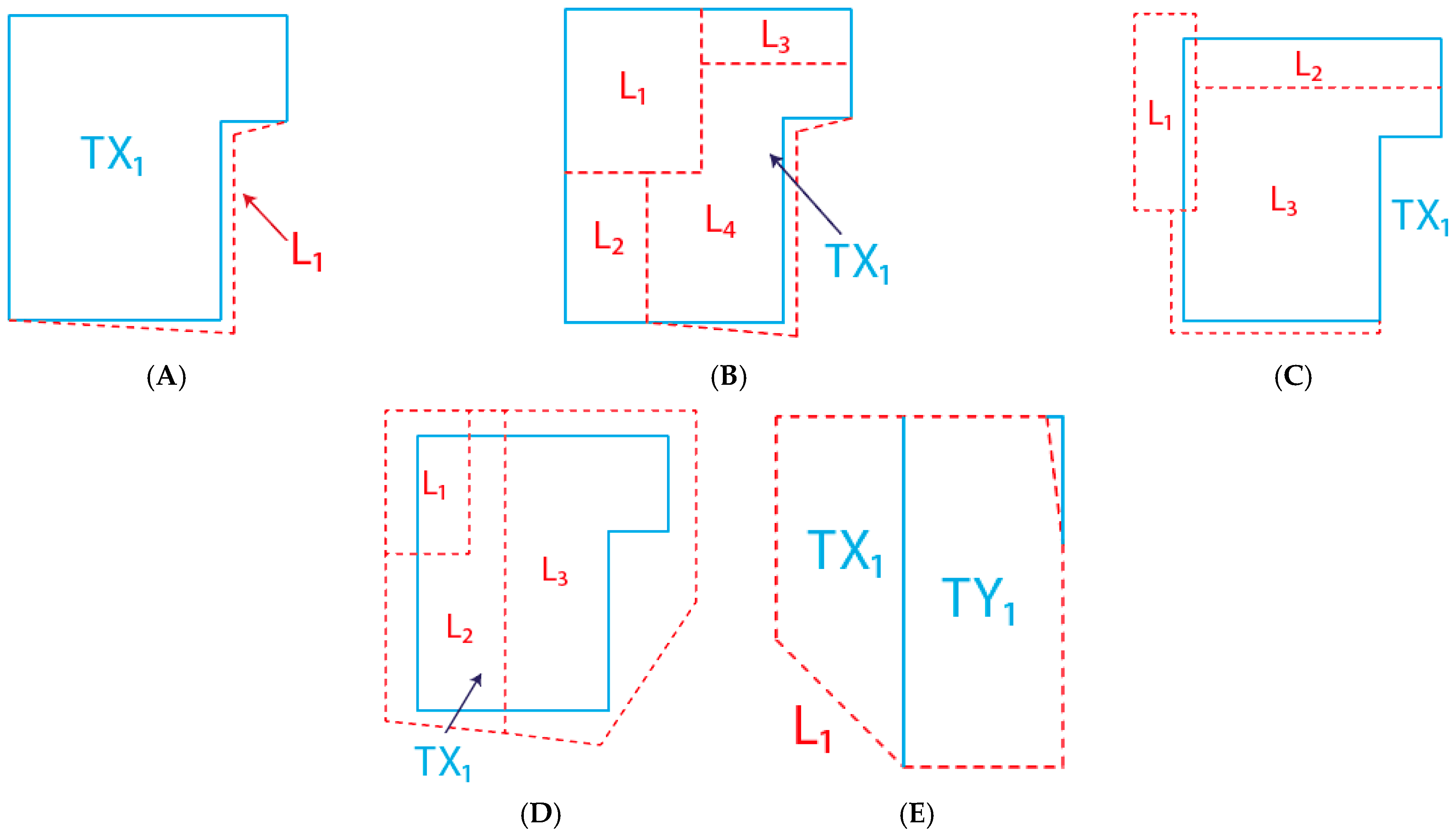
14Topologically class polygons into single parcel areas following the processes described below:
ProcessMethod
1Re-assign unique IDs of OS_Build and OS_Access_Build polygons according to neighbouring pBUILDINGS polygon with largest area
2Find pBUILDINGS objects with IDs different to IDs of neighbouring topological class polygons
3Use neighbouring IDs to link areas together; assign new ID to all polygons with any of the neighbouring IDs; iterate this process until no further polygon IDs can be re-assigned; re-assign topological class labels to OS_Access_Build if any polygons with new ID is this class, else re-assign class labels as OS_Build
4Assign IDs of OS_Build polygons to OS_Access polygons based upon majority shared border, and reclassify combined area as OS_Access_Build
5Merge remaining OS_Build polygons to OS_Access_Build polygons based upon majority shared border
6Re-classify remaining OS_Build polygons neighbouring Roadsides AND OS_Access_Build polygons as OS_Land_Parcels
7Re-classify remaining OS_Build polygons as OS_Islands
15Merge OS_Islands with neighbouring class polygons (excluding pWATER, pPATH, and Brownfield) based upon majority shared border; re-classify remaining OS as OS PARCELS if this condition is not satisfied; dissolve all polygons according to updated classification.
16Manually inspect OS PARCELS polygons in conjunction with May 2017 and Google Earth street-view imagery to assign appropriate ULU class labels; if OS PARCELS do not represent homogenous ULU class parcel area then re-classify as error parcels.
17Rectify error parcels by using polygons to select original contained OS MasterMap polygon areas; group error parcels into homogenous land parcel areas and assign appropriate class label.
18Merge remaining non-ULU class polygons (excluding pWATER) into neighbouring ULU polygons according to majority border relationship.
19Identify polygons below the minimum mapping unit of 45 m2 and merge with neighbouring class areas according to majority shared neighbouring border. The minimum mapping unit area (45 m2) was determined by a general observation that polygons of this size would contain 20 complete classification pixels and thus maintain the expected change detection accuracy of 85% when considering whole pixel numbers (85% of 20 is thus 17).
20Manually select pWATER areas that are neither water channels, canals, rivers, nor reservoirs (shared water utilities) and merge into neighbouring class polygons based upon majority shared boundary.
21Create parcel based building info features (see Table A16) for Residential polygons using Building Heights polygons by extracting building polygons with area ≥ 30 m2 (representing actual dwelling areas) contained inside Residential polygon areas.
22Classify ULU Residential polygons as follows:
ProcessMethod
1Select classification samples for Low-, Medium-, and High-density residential classes (using ancillary imagery and MasterMap polygons as a guide) and split into training and validation samples
2Use the random forest algorithm (see Table A17) to re-classify residential polygons ensuring overall classification accuracy ≥85%
3Manually re-classify (using ancillary imagery and OS MasterMap polygons as a guide) any residential polygons that do not contain Building Heights data
23Create final ULU class layer by ensuring topological errors are corrected, with updated ID values, polygon area, and length data attached.
Table A16. Parcel-based building info features for random forest classification.
FeatureMethod
MIN_HTMinimum dwelling building height
MAX_HTMaximum dwelling building height
AVE_HTAverage dwelling building height
RAN_HTDifference between MIN_HT and MAX_HT
MIN_ARMinimum dwelling building area
MAX_ARMaximum dwelling building area
AVE_ARAverage dwelling building area
RAN_ARDifference between MIN_AR and MAX_AR
MIN_VLMinimum dwelling building volume
MAX_VLMaximum dwelling building volume
AVE_VLAverage dwelling building volume
RAN_VLDifference between MIN_VL and MAX_VL
LOG_RATIO_AREALog of [parcel polygon area/Total residential dwelling area]
LOG_RATIO_VOLUMELog of [parcel polygon area/Total residential dwelling volume]
B_AVE_NBAverage number of dwellings per block
B_AVE_ARAverage area of block
B_MIN_ARMinimum residential block area
B_MAX_ARMaximum residential block area
B_RAN_ARDifference between B_MIN_AR and B_MAX_AR
B_AVE_HTAverage residential block height
B_MIN_HTMinimum residential block height
B_MAX_HTMaximum residential block height
B_RAN_HTDifference between B_MIN_HT and B_MAX_HT
B_AVE_VLAverage residential block volume
B_MIN_VLMinimum residential block volume
B_MAX_VLMaximum residential block volume
B_RAN_VLDifference between B_MIN_VL and B_MAX_VL
Table A17. Application of Random Forest to re-classify ULU Residential group parcel polygons.
StepDescription
1An initial 300 residential polygons were chosen using random selection (within quantiles for polygon areas) with class labels manually assigned. Due to the limited number of Residential—High (n = 26) samples obtained through this process, additional samples (n = 54; total of 80) were obtained for this class. Sample numbers for Residential—Sub-urban (n = 134) and Residential—Urban (n = 140) remained relatively even. A reasonable number of polygons for training the data were randomly split (within quantiles for polygon areas), ensuring a 75/25% split for training and validation polygons, respectively.
2The final random forest model was tuned with features (B_AVE_AR, AVE_VL, B_AVE_NB, AVE_AR, MAX_VL, and MAX_AR) selected using the VSURF() algorithm in addition to parameters: mtry = 1 and ntree = 1000. Overall accuracy on validation samples = 85.1% (kappa = 0.767).
3Residential polygons lacking appropriate classification feature data (186 out of 5867) were manually re-classified.

Appendix B.4. Validation of Urban Land Use Layer

As potential error may have occurred from the various methods used, final map accuracy was assessed using MasterMap topography layer sample polygons contained within ULU class areas as reference samples. The minimum number of validation samples was determined as n = 870 (30 per ULU class × 29 classes in total) based upon the minimum per class sample number rule to validate overall classification accuracy. Polygon samples were stratified within areal quintiles to ensure even distribution of polygon area sizes across ULU classes and were then compared to year 2017 multi-spectral imagery to assign a suitable ULU validation class label. Accuracy was then assessed using the error matrix method (see Table A18)
Table A18. Error matrix from ULU layer validation.
ULU GroupULU ClassUser Accuracy (%)Producer Accuracy (%)Class Confusion (Row-wise) Counts
BrownfieldBrownfield10097.1
CommercialCommercial93.993.9Public open space × 1|Residential—Low × 1
Community ServicesReligious facilities100100
Cultural facilities100100
Health care10097.1
Safety and well-being10097.1
Further education100100
Schools100100
IndustrialEnergy utilities90.9100Railways × 2|Woodland × 1
Industrial93.996.9Residential—Low × 2
Non-recreational Open SpaceAgriculture93.9100Health care × 1|Residential—Low × 1
Cemeteries100100
Water100100
Woodland90.9100Major roads × 1|Public open space × 1|Residential—Low × 1
Recreational Open SpacePublic open space93.993.9Residential—Low × 1|Roadside × 1
Sports facilities10097.1
Urban farming97.0100Sports facilities × 1
ResidentialResidential—Low84.471.1Residential—Medium × 5
Residential—Medium10080.5
Residential—High78.8100Residential—Low × 4|Residential—Medium × 3
TransportRailways87.993.5Commercial × 2|Brownfield × 1|Residential—Low × 1
Roadsides97.097.0Minor roads × 1
Limited access roads100100
Minor roads10097.1
Linking roads100100
Major roads10097.1
Motorways100100
Transport terminals100100
Car parking97.0100Industrial × 1
Overall accuracy = 96.6%; kappa = 0.96.

Appendix C

Appendix C.1. Polygon Overlap Comparison Process

OS land-line data [48] for the year 2000 provide the reference spatial data to backdate 2017 ULU information using polygon overlap methods. As real-world topographic features remain in position over time (e.g., parcel fence-line, road edge), the representative polyline or polygon line detail should also remain consistent between the OS land-line and MasterMap products [44]. Polygon-to-polygon comparison between OS datasets enables the identification of sub-ULU features that remain consistent in shape and spatial position over time [49].
Visual comparison of sub-2017 ULU OS MasterMap features (MM17) and LL00 polygons revealed both consistencies and inconsistencies in mapping detail between the datasets. As such, an automatic polygon comparison algorithm was developed to allow some degree of variance when assessing varying topological circumstances between corresponding polygon sets (Figure A3).
Figure A3. Topological circumstances when comparing overlapping polygon features. (A) High degree of overlap between TX1 (MM17) and L1 (LL00) polygons; (B) High degree of overlap between TX1 (MM17) and multiple L1-4 (LL00) polygons; (C) Varying degrees (low to high) of overlap between TX1 (MM17) and multiple L1-3 (LL00) polygons; (D) Low degree of overlap between TX1 (MM17) and multiple L1-3 (LL00) polygons; (E) High degree of overlap between multiple TX1, TY1 (MM17) and L1 (LL00) polygons.
Land 14 01077 g0a3
The polygon comparison algorithm works as follows. As shown in Figure A3A, the boundaries of Polygon TX1 (MM17 polygon of ULU class XULU) and L1 (LL00 polygon) mostly coincide, indicating a consistent land use feature over time. The degree of overlap is calculated as:
O v e r l a p = a r e a ( T X 1 ) a r e a ( L 1 )
In this instance, where O v e r l a p > C . T . (where C . T . = user-defined conditional parameter defining the proportion of overlap required between comparative polygons), this is classified as a no-change ULU sample area. Figure A3B describes a more complex topological arrangement, as TX1 coincides with combined boundaries of LL00 polygons {L1, L2, L3, L4}. This could indicate land use change as year 2000 features of different land use have been combined into a single 2017 ULU area or that consistent land use features have not been digitised in the 2017 MasterMap layer. Examination of both datasets indicated that the second condition prevails in most circumstances, therefore the degree of overlap between polygons A and {B1, B2, B3, B4} in this instance is calculated as:
O v e r l a p = a r e a ( L 1 , L 2 , L 3 , L 4 ) a r e a ( T X 1 )
Therefore, if O v e r l a p > C . T . , then polygons {B1, B2, B3, B4} are classified as consistent ULU sample areas. In instances where comparison polygons share similar areas but have different shapes, and do not consistently overlap, use of the Overlap function as defined in A and B may incorrectly indicate a no-change ULU sample area (Figure A3C). This is controlled in the process as follows:
(i)
Sub-set LL00 polygons that intersect T X 1 :
L L 00 = { L 1 , L 2 , L m a x }
L L _ i n t = { L L 00   : L L 00 T X 1 }
(ii.)
Select LL00 polygons if ratio of intersected area to LL00 polygon area is >C.T.
L L _ t e s t = L L _ i n t   : a r e a L L _ i n t T X 1 a r e a L L _ i n t > C . T .
(iii.)
Calculate Overlap:
O v e r l a p = a r e a ( L L _ t e s t ) a r e a ( T X 1 )
In this instance, the conditional process removes L1 from the Overlap comparison, which overlaps TX1 slightly due to a slight change in boundary position. The remaining L2 and L3 polygons are relatively contiguous with the TX1 polygon and are thus selected as consistent ULU sample areas. In Figure A3D it appears that there has been significant change for the representative polygon area. This may not indicate land use change in itself as neighbouring MM17 features may have been simply re-arranged to define the same land use, i.e., reconfiguration of buildings on an existing school site. However, establishing different orders of polygon neighbours (i.e., identifying which set of multiple polygons overlaps with another set of multiple polygons) requires significant additional computation using the algorithmic process. Thus O v e r l a p is simply calculated for either a ONE reference polygon to ONE test polygon or a ONE reference polygon to MANY test polygons relationship. In this case, reasoning would suggest that no LL00 polygon should be selected as a no-change ULU sample. However, this is dependent on how lenient the conditional overlap threshold ( C . T . ) is. In Figure A3E, the roles of MM17 and LL00 polygons are reversed, therefore O v e r l a p is calculated by reversing the numerator and denominator references in Equation (A1). However, L 1 may not be considered a no-change sample area in this instance as:
  U L U   o f   T X 1   U L U   o f   T Y 1     o r   [   X Y   ]
L1 is assumed to be a single land use feature comprising different 2017 ULU classes, as such it appears that this area in 2000 has now been sub-divided for different ULU purposes in 2017 and has thus changed ULU categorisation over the study period. This process was implemented using programming language version 3.6 [50], with the code provided in Appendix C.2 with definition of the C.T. value in Appendix C.3.

Appendix C.2. Polygon Overlap Comparison Algorithm

The following code can be copied as R script. No libraries are required for the algorithm to function.
  • # ~~~~~~~~~~~~~~~~~~~~~~~~~~~~~~~~~~~~~~~~~~~~~~~~~~~~~~~~~~~~~~
  • # Overlap algorithm—function code with instructions (lines starting with ‘#’ are comments
  • # and not functioning script)
  • # Author: Fraser Baker; Date: 7th February 2020
  • # ~~~~~~~~~~~~~~~~~~~~~~~~~~~~~~~~~~~~~~~~~~~~~~~~~~~~~~~~~~~~~~
  • # Pre-processing—requires input data as follows:
  • #
  • # -> REFERENCE POLYGONS: THESE ARE POLYGONS WITH LAND-USE CLASS
  • # LABELS; MUST CONTAIN UNIQUE POLYGON ID REFERENCE (REF.ID),
  • # POLYGON AREA (AREA.REF) AND LAND-USE CLASS LABEL (CLASS)
  • #
  • # -> TEST POLYGONS: THESE ARE POLYGONS WITHOUT LAND-USE CLASS
  • # LABELS; MUST CONTAIN UNIQUE POLYGON ID REFERENCE (TES.ID)
  • # AND POLYGON AREA (AREA.TES)
  • #
  • # Intersect REFFERENCE and TEST POLYGONS to create new dataset
  • # with the required fields below:
  • #
  • # REF.ID = ID OF INTERSECTED REFERENCE POLYGON
  • # TES.ID = ID OF INTERSECTED TEST POLYGON
  • # AREA.INT = AREA OF POLYGON INTERSECTION
  • # AREA.REF = ORIGINAL AREA OF INTERSECTED REFERENCE POLYGON
  • # AREA.TES = ORIGINAL AREA OF INTERSECTED TEST POLYGON
  • # RATIO.TES = AREA.INT/AREA.TES
  • # RATIO.REF = AREA.INT/AREA.REF
  • # CLASS = LAND-USE CLASS ASSIGNED TO REFERENCE POLYGON
  • #
  • # data.frame (DF) required from this dataset only
  • # ~~~~~~~~~~~~~~~~~~~~~~~~~~~~~~~~~~~~~~~~~~~~~~~~
  • # overlap() function defined below—requires following inputs from user:
  • #
  • # DF = data.frame of REFERENCE to TEST polygon intersection
  • # ID = unique ID of REFERENCE polygon under investigation
  • # c.t = conditional threshold to assess polygon overlap
  • #
  • # all other variables in function call should be assigned NULL
  • #
  • overlap <- function(DF,ID,c.t,rel.REF.2.TES = NULL,TES.sub.of.RES = NULL,
  • a = NULL,a.TES.ov.REF = NULL,a.REF.ov.TES = NULL){
  • #
  • a <- DF[DF$REF.ID%in%ID,] #subset main dataframe according to ID of
  • # REFERENCE polygon under investigation
  • #
  • if(length(a$TES.ID)>1){
  • # If a has multiple records then REFERENCE polygon is subdivided by
  • # multiple TEST polygons
  • #
  • a.REF.ov.TES <- a[a$RATIO.REF>c.t,] # subset all records where RATIO.TES > c.t
  • #
  • if(length(a.TES.ov.REF$TES.ID) > 0){ # assess if any records for TEST polygons remain
  • rel.REF.2.TES <- ifelse((sum(a.TES.ov.REF$AREA.TES)/unique(a.TES.ov.REF$AREA.REF))>c.t,1,0)
  • # If TRUE TEST polygons form part of group that sub-divides and overlaps a REFERENCE
  • # polygon within threshold tolerance; CON = 1 in this case
  • #
  • TES.sub.of.REF <- unique(a.REF.ov.TES$TES.ID) # store ID’s of TEST polygons intersected
  • # with the REFERENCE polygon
  • }
  • } else {
  • # If a has single record then this this suggests REFERENCE may be matched to a single
  • # TEST polygon or forms a group of REFERENCE polygons that sub-divides a single TEST
  • # polygon
  • a.TES.ov.REF <- DF[DF$TES.ID%in%a$TES.ID,] # subset all records from main dataframe by
  • # TEST.ID in a
  • #
  • a.TES.ov.REF <- a.TES.ov.REF[a.REF.ov.TES$RATIO.REF > c.t,] # subset all records where
  • # RATIO.REF > c.t.
  • #
  • if(length(a.TES.ov.REF$REF.ID) > 0){ #
  • if((sum(a.TES.ov.REF$AREA.REF)/unique(a.TES.ov.REF$AREA.REF)) > c.t){
  • # If TRUE REFERENCE polygons form part of group that sub-divides and
  • # overlaps a TEST polygon within threshold tolerance
  • if(length(unique(a.TES.ov.REF$CLASS))==1){ # multiple land-use classes are not acceptable
  • #
  • rel.REF.2.TES <- ifelse(length(a.TES.ov.REF$REF.ID)>1,2,1)
  • # If TRUE TEST polygon is part of group that sub-divides
  • # and overlaps REFERENCE polygon within threshold tolerance: CON = 2;
  • # ELSE REFERENCE polygon overlaps single TEST polygon only: CON = 1
  • }
  • #
  • TES.sub.of.REF <- unique(a.TES.ov.REF$TES.ID) # store relevant ID values for TEST polygons
  • #
  • }
  • }
  • }
  • #
  • return(list(REF.ID=ID,CLASS=unique(a$CLASS),RL.CON=rel.REF.2.TES,
  • TES.ID=TES.sub.of.REF))
  • # function returns list for input REFERENCE polygon with: REF.ID;
  • # CLASS (Class of REFERENCE polygon);RL.CON (relative condition of overlap);
  • # TES.ID (IDs of TEST polygons intersected to REFERENCE polygons)
  • }
  • #
  • # Note: for large datasets that parrallel processing may be required to loop through all
  • # unique REFERENCE polygon IDs

Appendix C.3. Definition of the C.T. Parameter in the Polygon Algorithm

Sensitivity analysis was conducted to identify an optimal C . T . value that produced a reasonable trade-off between sample error rate and total number of correctly identified ULU class polygons. For this, 300 ULU polygons were randomly selected as validation areas and were classed as either no change (n = 242), partially changed (n = 18), or fully changed (n = 40) when comparing changes in features between overlapping 2000 and 2017 imagery. The overlap algorithm was then run for no-change and full-change MM17 polygons, using a sequence of test C . T . values defined as:
a 1 = 85 100 ;   a n = a n 1 + 1 1,000,000 ; f o r   n   100
The correct polygon recall rate was therefore calculated as the percentage of actual no-change polygons identified by the algorithm for each test C . T . value. The process was also run on the full dataset for C . T . values 0.85, 0.90, and 0.999999. This examined how the proportion of identified no-change MM17 polygons varies according to stringency in C . T . value. Three values were tested due to the computational time required to implement this process for full polygon datasets. Comparison between the error and no-change percentage determined a suitable C . T . value for final sample calculation. The final LL00 sample dataset was then validated using an independent sample of ULU class MM17 polygons (n = 384). Actual ULU class labels were recorded for sample polygons in order to populate an error matrix with kappa statistics [91,101] and determine overall accuracy of the chosen O v e r l a p   C . T . value.
The estimated recall accuracy of the C.T. threshold of the Overlap algorithm is above 98% for all threshold settings (Figure A4). Totals of 63.5%, 60.2%, and 38% of total MM17 candidate sample polygons (n = 662,828) were identified as no-change areas for C.T. threshold values 0.85, 0.9, and >0.999, respectively. The first two values return a considerable sample area when considering that the estimated percentage of actual no-change ULU areas is 80.7%.
Figure A4. Impact of Overlap threshold upon Overlap algorithm recall accuracy.
Land 14 01077 g0a4

Appendix D

Implementation of Error Adjustment Method to Estimate Net UGBI Change

Theory and development of the error adjustment method are provided by [52]. The following practical example demonstrates how this method was implemented in this investigation. The first stage of the method requires an independent accuracy assessment of the change layer using an error matrix. Final class area estimates are also required to calculate proportional class coverage for the area under investigation. Dummy information is demonstrated in Table A19 for the change detection classes used in this investigation.
Table A19. Example error matrix for error adjustment method.
LossGainUGBI StasisNon-UGBI StasisTotalClass Area (m2)Proportion of Total Area
Loss115082125767,9930.13
Gain097226125432,5670.08
GBI stasis5324112502,007,9210.35
Non-GBI stasis6202422502,505,4410.44
Totals5,713,9221
The second stage thus requires this information to calculate error-adjusted class proportions of total area per class:
p . j = i W i n i j n i
where p . j is the error-adjusted proportion per column-wise class j; W i is the proportion of total area for row-wise class i; n i j is error matrix count for row-wise class i and column-wise class j; n i is total row cell count for row-wise class i. Using this equation an adjusted error matrix is calculated (see below). For each cell the proportion of total area is calculated according to appropriate error count, with column sums per class providing the total error-adjusted area proportion per class (Table A20).
Table A20. Example error-adjusted proportion of total class area for change classes.
LossGainGBI StasisNon-GBI Stasis
Loss0.1240.0000.0090.002
Gain0.0000.0590.0130.004
GBI stasis0.0060.0050.3380.002
Non-GBI stasis0.0100.0030.0000.425
Error-adjusted proportion of total area0.140.070.360.43
Error-adjusted area (m2)801,607.0382,778.32,059,179.62,470,357.1
As shown above the error-adjusted areas per class (rows) are calculated by multiplying the error-adjusted proportions per respective reference class (columns) by the total class area. To calculate confidence interval estimates, first the standard error of the error-adjusted proportion is found using the following equation:
S ( p . j ) = i = 1 q W i 2 n i j n i 1 n i j n i n i 1
where q is the total number of classes. For example, the standard error of the error-adjusted proportion for the loss class is calculated as follows:
S L o s s = 0.13 2 115 125   1 115 125 125 1 + 0.08 2 0 125   1 0 125 125 1 + 0.35 2 5 250   1 5 250 250 1 + 0.44 2 6 250   1 6 250 250 1 1 2 = 0.0075
Confidence interval estimates of error-adjusted area are calculated by converting the standard error proportion into an areal figure and multiplying this figure by the z-score for the required confidence level (e.g., 95% here)—see below:
A r e a S L o s s = z · A r e a t o t · S L o s s = 1.96 · 5713922 · 0.0075 = ± 83991.7 m 2
Error-adjusted area estimates are thus required for loss and gain classes only. The total change area is calculated using the high and low class estimates for both classes. Central, upper, and lower net change are calculated as follows:
 N e t =  G a i n  L o s s = 382778.3 801607.0 = 418828.7 m 2
 U p p e r N e t =  G a i n + A r e a S G a i n  L o s s A r e a S L o s s = 382778.3 + 58402.7 801607.0 83991.7 = 276434 m 2
 L o w e r N e t =  N e t +  N e t  U p p e r N e t = 418828.7 + 418828.7 276434 = 561223.1 m 2
This process is calculated for all areas of analysis: (i) study area; (ii) analysis cells; (iii) ULU class samples. Error matrix values remain consistent in all cases, whilst change class and total area values vary between analysis areas. Upper and lower net change values thus confine the boundaries of potential UGBI change. If lower net change ≤ 0 ≤ upper net change for the analysis area then a no-change (stasis) condition is recorded.

Appendix E

Insignificant Differences Between Urban Land Use Classes Within Urban Land Use Groups

Insignificant differences between ULU classes within ULU groups may indicate some redundancy in using multiple sub-ULU group classes, where two or more ULU classes could be merged to identify a consistent sub-group UGBI change.
ULU Class 1ULU Class 2p-ValuesULU Group
AgricultureWater1Non-public open space
AgricultureWoodland0.1Non-public open space
Further educationHealth care1Community services
Further educationReligious facilities1Community services
Further educationSchools1Community services
Health careReligious facilities1Community services
Health careSchools1Community services
Limited access roadsRailways1Transport
Linking roadsMinor roads1Transport
Linking roadsMotorways1Transport
Linking roadsRoadsides1Transport
Major roadsMotorways1Transport
Minor roadsMotorways0.8Transport
Minor roadsRoadsides1Transport
MotorwaysRoadsides1Transport
Note: Insignificant differences detected using Pairwise Wilcoxon–Mann–Whitney U test; R programming language version 3.6 [50].

References

  1. Carter, J.G.; Cavan, G.; Connelly, A.; Guy, S.; Handley, J.; Kazmierczak, A. Climate change and the city: Building capacity for urban adaptation. Prog. Plan. 2015, 95, 1–66. [Google Scholar] [CrossRef]
  2. Andreucci, M.B. Progressing green infrastructure in Europe. WIT Trans. Ecol. Environ. 2013, 179, 413–422. [Google Scholar]
  3. Evans, D.L.; Falagán, N.; Hardman, C.A.; Kourmpetli, S.; Liu, L.; Mead, B.R.; Davies, J.A.C. Ecosystem service delivery by urban agriculture and green infrastructure–a systematic review. Ecosyst. Serv. 2022, 54, 101405. [Google Scholar] [CrossRef]
  4. Farina, G.; Le Coent, P.; Hérivaux, C. Do urban environmental inequalities influence demand for nature based solutions? Ecol. Econ. 2024, 224, 108298. [Google Scholar] [CrossRef]
  5. Chen, B.; Nie, Z.; Chen, Z.; Xu, B. Quantitative estimation of 21st-century urban greenspace changes in Chinese populous cities. Sci. Total Environ. 2017, 609, 956–965. [Google Scholar] [CrossRef] [PubMed]
  6. Dallimer, M.; Tang, Z.; Bibby, P.R.; Brindley, P.; Gaston, K.J.; Davies, Z.G. Temporal changes in greenspace in a highly urbanized region. Biol. Lett. 2011, 7, 763–766. [Google Scholar] [CrossRef]
  7. Haaland, C.; van Den Bosch, C.K. Challenges and strategies for urban green-space planning in cities undergoing densification: A review. Urban For. Urban Green. 2015, 14, 760–771. [Google Scholar] [CrossRef]
  8. Richards, D.R.; Passy, P.; Oh, R.R. Impacts of population density and wealth on the quantity and structure of urban green space in tropical Southeast Asia. Landsc. Urban Plan. 2017, 157, 553–560. [Google Scholar] [CrossRef]
  9. Rodríguez, J.P.; Beard, T.D., Jr.; Bennett, E.M.; Cumming, G.S.; Cork, S.J.; Agard, J.; Dobson, A.P.; Peterson, G.D. Trade-offs across space, time, and ecosystem services. Ecol. Soc. 2006, 11, 28. [Google Scholar] [CrossRef]
  10. De Groot, R.S.; Alkemade, R.; Braat, L.; Hein, L.; Willemen, L. Challenges in integrating the concept of ecosystem services and values in landscape planning, management and decision making. Ecol. Complex. 2010, 7, 260–272. [Google Scholar] [CrossRef]
  11. Mell, I.; Clement, S. Progressing green infrastructure planning: Understanding its scalar, temporal, geo-spatial and disciplinary evolution. Impact Assess. Proj. Apprais. 2020, 38, 449–463. [Google Scholar] [CrossRef]
  12. Fisher, P.F.; Comber, A.J.; Wadsworth, R. Land use and land cover: Contradiction or complement. In Re-Presenting GIS; John Wiley and Sons Ltd.: Hoboken, NJ, USA, 2005; pp. 85–98. [Google Scholar]
  13. Barker, K. Barker Review of Land Use Planning: Final Report, Recommendations; The Stationery Office: Norwich, UK, 2006. [Google Scholar]
  14. Burkhard, B.; Kroll, F.; Nedkov, S.; Müller, F. Mapping ecosystem service supply, demand and budgets. Ecol. Indic. 2012, 21, 17–29. [Google Scholar] [CrossRef]
  15. Hasan, S.; Shi, W.; Zhu, X. Impact of land use land cover changes on ecosystem service value–A case study of Guangdong, Hong Kong, and Macao in South China. PLoS ONE 2020, 15, e0231259. [Google Scholar] [CrossRef] [PubMed]
  16. Sutton, P.C.; Anderson, S.J. Holistic valuation of urban ecosystem services in New York City’s Central Park. Ecosyst. Serv. 2016, 19, 87–91. [Google Scholar] [CrossRef]
  17. Preston, P.D.; Dunk, R.M.; Smith, G.R.; Cavan, G. Not all brownfields are equal: A typological assessment reveals hidden green space in the city. Landsc. Urban Plan. 2023, 229, 104590. [Google Scholar] [CrossRef]
  18. Warhurst, J.R.; Parks, K.E.; McCulloch, L.; Hudson, M.D. Front gardens to car parks: Changes in garden permeability and effects on flood regulation. Sci. Total Environ. 2014, 485, 329–339. [Google Scholar] [CrossRef]
  19. Lin, L.; Zhang, C. Land parcel identification. In Agro-Geoinformatics: Theory and Practice; Springer: Cham, Switzerland, 2021; pp. 163–174. [Google Scholar]
  20. Cavan, G.; Baker, F.; Tzoulas, K.; Smith, C.L. Manchester: The role of urban domestic gardens in climate adaptation and resilience. In Urban Climate Science for Planning Healthy Cities; Springer: Cham, Switzerland, 2021; pp. 99–118. [Google Scholar]
  21. Pauleit, S.; Ennos, R.; Golding, Y. Modeling the environmental impacts of urban land use and land cover change—A study in Merseyside, UK. Landsc. Urban Plan. 2005, 71, 295–310. [Google Scholar] [CrossRef]
  22. Wellmann, T.; Schug, F.; Haase, D.; Pflugmacher, D.; van der Linden, S. Green growth? On the relation between population density, land use and vegetation cover fractions in a city using a 30-years Landsat time series. Landsc. Urban Plan. 2020, 202, 103857. [Google Scholar] [CrossRef]
  23. Dobbs, C.; Hernández-Moreno, Á.; Reyes-Paecke, S.; Miranda, M.D. Exploring temporal dynamics of urban ecosystem services in Latin America: The case of Bogota (Colombia) and Santiago (Chile). Ecol. Indic. 2018, 85, 1068–1080. [Google Scholar] [CrossRef]
  24. Cortinovis, C.; Geneletti, D. Ecosystem services in urban plans: What is there, and what is still needed for better decisions. Land Use Policy 2018, 70, 298–312. [Google Scholar] [CrossRef]
  25. Lam, S.T.; Conway, T.M. Ecosystem services in urban land use planning policies: A case study of Ontario municipalities. Land Use Policy 2018, 77, 641–651. [Google Scholar] [CrossRef]
  26. Reba, M.; Seto, K.C. A systematic review and assessment of algorithms to detect, characterize, and monitor urban land change. Remote Sens. Environ. 2020, 242, 111739. [Google Scholar] [CrossRef]
  27. Morin, E.; Herrault, P.A.; Guinard, Y.; Grandjean, F.; Bech, N. The promising combination of a remote sensing approach and landscape connectivity modelling at a fine scale in urban planning. Ecol. Indic. 2022, 139, 108930. [Google Scholar] [CrossRef]
  28. Almeida, C.R.D.; Teodoro, A.C.; Gonçalves, A. Study of the urban heat island (UHI) using remote sensing data/techniques: A systematic review. Environments 2021, 8, 105. [Google Scholar] [CrossRef]
  29. Zhu, Q.; Guo, X.; Li, Z.; Li, D. A review of multi-class change detection for satellite remote sensing imagery. Geo-Spat. Inf. Sci. 2024, 27, 1–15. [Google Scholar] [CrossRef]
  30. Domingo, D.; Palka, G.; Hersperger, A.M. Effect of zoning plans on urban land-use change: A multi-scenario simulation for supporting sustainable urban growth. Sustain. Cities Soc. 2021, 69, 102833. [Google Scholar] [CrossRef]
  31. Kudas, D.; Wnęk, A.; Hudecová, Ľ.; Fencik, R. Spatial Diversity Changes in Land Use and Land Cover Mix in Central European Capitals and Their Commuting Zones from 2006 to 2018. Sustainability 2024, 16, 2224. [Google Scholar] [CrossRef]
  32. Huang, H.; Chen, Y.; Clinton, N.; Wang, J.; Wang, X.; Liu, C.; Gong, P.; Yang, J.; Bai, Y.; Zheng, Y.; et al. Mapping major landcover dynamics in Beijing using all Landsat images in Google Earth Engine. Remote Sens. Environ. 2017, 202, 166–176. [Google Scholar] [CrossRef]
  33. Liu, S.; Marinelli, D.; Bruzzone, L.; Bovolo, F. A review of change detection in multitemporal hyperspectral images: Current techniques, applications, and challenges. IEEE Geosci. Remote Sens. Mag. 2019, 7, 140–158. [Google Scholar] [CrossRef]
  34. ONS (Office for National Statistics). How the Population Changed in Manchester: Census 2021. 28 June 2022. Available online: https://www.ons.gov.uk/visualisations/censuspopulationchange/E08000003/ (accessed on 23 March 2025).
  35. Manchester City Council. Manchester Green and Blue Infrastructure Strategy: Implementation Plan Refresh 2021–25. 2022. Available online: https://www.manchester.gov.uk/downloads/download/7456/2022_green_and_blue_infrastructure_refresh (accessed on 23 March 2025).
  36. Airbus. Spot 7 imagery [Data Download]. 2018. Adapted with Permission from © Airbus DS (2018). Licenced from ESA [European Space Agency]. 2018. Available online: http://open.esa.int/ (accessed on 12 March 2018).
  37. McDonald, R.I. Conservation for Cities: How to Plan & Build Natural Infrastructure; Island Press: Washington, DC, USA, 2015. [Google Scholar]
  38. Da Silva, J.M.C.; Wheeler, E. Ecosystems as infrastructure. Perspect. Ecol. Conserv. 2017, 15, 32–35. [Google Scholar] [CrossRef]
  39. Getmapping. Aerial Data—High Resolution Imagery [Data Download]. Adapted with permission from © Getmapping (2019). 2019. Available online: https://www.getmapping.co.uk/aerial-content/ (accessed on 29 May 2019).
  40. Persson, M.; Lindberg, E.; Reese, H. Tree species classification with multi-temporal Sentinel-2 data. Remote Sens. 2018, 10, 1794. [Google Scholar] [CrossRef]
  41. Peiman, R. Pre-classification and post-classification change-detection techniques to monitor land cover and land-use change using multi-temporal Landsat imagery: A case study on Pisa Province in Italy. Int. J. Remote Sens. 2011, 32, 4365–4381. [Google Scholar] [CrossRef]
  42. Jensen, J.R. Digital Image Processing: A Remote Sensing Perspective; Prentice Hall: Upper Saddle River, NJ, USA, 2005. [Google Scholar]
  43. Fuller, R.M.; Smith, G.M.; Devereux, B.J. The characterisation and measurement of land cover change through remote sensing: Problems in operational applications? Int. J. Appl. Earth Obs. Geoinf. 2003, 4, 243–253. [Google Scholar] [CrossRef]
  44. OS [Ordnance Survey]. OS MasterMap Topography Layer [Data Download]. 2017. Adapted with Permission from © Ordnance Survey (2020). Licenced from Edina Digimap AC0000851941. 2020. Available online: https://digimap.edina.ac.uk/ (accessed on 18 January 2020).
  45. Serra, P.; Pons, X.; Sauri, D. Post-classification change detection with data from different sensors: Some accuracy considerations. Int. J. Remote Sens. 2003, 24, 3311–3340. [Google Scholar] [CrossRef]
  46. Copernicus Land Monitoring Service. Urban Atlas. 2020. Available online: https://land.copernicus.eu/local/urban-atlas (accessed on 22 June 2020).
  47. Harrison, A.R. National Land Use Database: Land Use and Land Cover Classification; LandInform Ltd: Bristol, UK, 2006. [Google Scholar]
  48. OS [Ordnance Survey]. Land-Line [Data Download]. 2000. Adapted with Permission from © Ordnance Survey (2020). Licenced from Edina Digimap AC0000851941. 2020. Available online: https://digimap.edina.ac.uk/ (accessed on 18 January 2020).
  49. Aspinall, R.J.; Hill, M. Land cover change: A method for assessing the reliability of land cover changes measured from remotely-sensed data. In Proceedings of the IGARSS’97. 1997 IEEE International Geoscience and Remote Sensing Symposium Proceedings. Remote Sensing-A Scientific Vision for Sustainable Development, Singapore, 3–8 August 1997; Volume 1, pp. 269–271. [Google Scholar]
  50. R Core Team. R: A Language and Environment for Statistical Computing; R Foundation for Statistical Computing: Vienna, Austria, 2022; Available online: https://www.r-project.org/ (accessed on 12 May 2025).
  51. Baker, F.; Smith, G.R.; Marsden, S.J.; Cavan, G. Mapping regulating ecosystem service deprivation in urban areas: A transferable high-spatial resolution uncertainty aware approach. Ecol. Indic. 2021, 121, 107058. [Google Scholar] [CrossRef]
  52. Olofsson, P.; Foody, G.M.; Stehman, S.V.; Woodcock, C.E. Making better use of accuracy data in land change studies: Estimating accuracy and area and quantifying uncertainty using stratified estimation. Remote Sens. Environ. 2013, 129, 122–131. [Google Scholar] [CrossRef]
  53. Swinney, P.; Thomas, E. A Century of Change in Manchester. 2015. Available online: https://www.centreforcities.org/reader/a-century-of-cities/3-are-cities-bound-by-these-pathways/1-a-century-of-change-in-manchester/ (accessed on 2 May 2020).
  54. Smith, A. The development of “sports-city” zones and their potential value as tourism resources for urban areas. Eur. Plan. Stud. 2010, 18, 385–410. [Google Scholar] [CrossRef]
  55. Urban Splash. New Islington, Manchester. 2020. Available online: https://www.urbansplash.co.uk/regeneration/projects/new-islington (accessed on 15 May 2020).
  56. Kirby, D. Revealed: The trees on our streets are being felled at a rate of 58 a day. I-News, 31 March 2017. Available online: https://inews.co.uk/news/environment/revealed-suburban-trees-felled-rate-58-day-527251 (accessed on 2 February 2020).
  57. Salmond, J.A.; Tadaki, M.; Vardoulakis, S.; Arbuthnott, K.; Coutts, A.; Demuzere, M.; Dirks, K.N.; Heaviside, C.; Lim, S.; Macintyre, H.; et al. Health and climate related ecosystem services provided by street trees in the urban environment. Environ. Health 2016, 15, 95–111. [Google Scholar] [CrossRef]
  58. Perry, T.; Nawaz, R. An investigation into the extent and impacts of hard surfacing of domestic gardens in an area of Leeds, United Kingdom. Landsc. Urban Plan. 2008, 86, 1–13. [Google Scholar] [CrossRef]
  59. Verbeeck, K.; Van Orshoven, J.; Hermy, M. Measuring extent, location and change of imperviousness in urban domestic gardens in collective housing projects. Landsc. Urban Plan. 2011, 100, 57–66. [Google Scholar] [CrossRef]
  60. Whitford, V.; Ennos, A.R.; Handley, J.F. “City form and natural process”—Indicators for the ecological performance of urban areas and their application to Merseyside, UK. Landsc. Urban Plan. 2001, 57, 91–103. [Google Scholar] [CrossRef]
  61. Bibby, P.; Henneberry, J.; Halleux, J.M. Under the radar? ‘Soft’ residential densification in England, 2001–2011. Environ. Plan. B Urban Anal. City Sci. 2020, 47, 102–118. [Google Scholar] [CrossRef]
  62. Sayce, S.; Walford, N.; Garside, P. Residential development on gardens in England: Their role in providing sustainable housing supply. Land Use Policy 2012, 29, 771–780. [Google Scholar] [CrossRef]
  63. Osborne, L.P.; Cushing, D.F.; Washington, T.L. Where have all the backyards gone? The decline of usable residential greenspace in Brisbane, Australia. Aust. Plan. 2021, 57, 100–113. [Google Scholar] [CrossRef]
  64. Sainsbury, L.B.; Slater, D. Changes in paved space, green infrastructure and tree canopy cover in front gardens: A case study of two contrasting housing estates in Liverpool, England. Arboric. J. 2023, 45, 152–172. [Google Scholar] [CrossRef]
  65. Simpson, T.J.; Francis, R.A. Artificial lawns exhibit increased runoff and decreased water retention compared to living lawns following controlled rainfall experiments. Urban For. Urban Green. 2021, 63, 127232. [Google Scholar] [CrossRef]
  66. Dewaelheyns, V.; Kerselaers, E.; Rogge, E. A toolbox for garden governance. Land Use Policy 2016, 51, 191–205. [Google Scholar] [CrossRef]
  67. Goddard, M.A.; Dougill, A.J.; Benton, T.G. Scaling up from gardens: Biodiversity conservation in urban environments. Trends Ecol. Evol. 2010, 25, 90–98. [Google Scholar] [CrossRef]
  68. Kabisch, N. Ecosystem service implementation and governance challenges in urban green space planning—The case of Berlin, Germany. Land Use Policy 2015, 42, 557–567. [Google Scholar] [CrossRef]
  69. Whitten, M. Blame it on austerity? Examining the impetus behind London’s changing green space governance. People Place Policy 2019, 12, 204–224. [Google Scholar] [CrossRef]
  70. De Bell, S.; White, M.; Griffiths, A.; Darlow, A.; Taylor, T.; Wheeler, B.; Lovell, R. Spending time in the garden is positively associated with health and wellbeing: Results from a national survey in England. Landsc. Urban Plan. 2020, 200, 103836. [Google Scholar] [CrossRef]
  71. Amegah, A.K.; Yeboah, K.; Owusu, V.; Afriyie, L.; Kyere-Gyeabour, E.; Appiah, D.C.; Osei-Kufuor, P.; Annim, S.K.; Agyei-Mensah, S.; Mudu, P. Socio-demographic and neighbourhood factors influencing urban green space use and development at home: A population-based survey in Accra, Ghana. PLoS ONE 2023, 18, e0286332. [Google Scholar] [CrossRef]
  72. Haase, D.; Gaeva, D. Allotments for all? Social–environmental values of urban gardens for gardeners and the public in cities: The example of Berlin, Germany. People Nat. 2023, 5, 1207–1219. [Google Scholar] [CrossRef]
  73. Groundwork. Ignition: Nature Based Solutions for Greater Manchester. 2020. Available online: https://www.groundwork.org.uk/greatermanchester/gm-about/our-impact-gm/ (accessed on 14 May 2020).
  74. City of Trees. About City of Trees. 2025. Available online: https://www.cityoftrees.org.uk/about (accessed on 23 March 2025).
  75. Wang, J.; Bretz, M.; Dewan, M.A.A.; Delavar, M.A. Machine learning in modelling land-use and land cover-change (LULCC): Current status, challenges and prospects. Sci. Total Environ. 2022, 822, 153559. [Google Scholar] [CrossRef]
  76. Chaturvedi, V.; de Vries, W.T. Machine learning algorithms for urban land use planning: A review. Urban Sci. 2021, 5, 68. [Google Scholar] [CrossRef]
  77. GMCA (Greater Manchester Combined Authority). Greater Manchester Five-Year Environment Plan 2025–2030. 2024. Available online: https://www.greatermanchester-ca.gov.uk/media/alnl0fsy/gmca_5-year-plan_final_digital_v3-ua.pdf (accessed on 30 April 2025).
  78. DEFRA (Department for Environment, Food & Rural Affairs). Understanding Biodiversity Net Gain. 21 February 2023. Available online: https://www.gov.uk/guidance/understanding-biodiversity-net-gain (accessed on 30 April 2025).
  79. Boyd, E.H.; Leigh, G.; Sutton, J. The London Climate Resilience Review; Mayor of London Office: London, UK, 2024.
  80. Cameron, R. “Do we need to see gardens in a new light?” Recommendations for policy and practice to improve the ecosystem services derived from domestic gardens. Urban For. Urban Green. 2023, 80, 127820. [Google Scholar] [CrossRef]
  81. Gu, Z.; Zeng, M. The use of artificial intelligence and satellite remote sensing in land cover change detection: Review and perspectives. Sustainability 2024, 16, 274. [Google Scholar] [CrossRef]
  82. Hijmans, R.J. raster: Geographic Data Analysis and Modeling. R Package Version 3.3-13. 2020. Available online: https://CRAN.R-project.org/package=raster (accessed on 18 January 2020).
  83. Airbus. Pléiades User Guide & SPOT 6/7 User Guide. 2020. Available online: https://www.intelligence-airbusds.com/docs/9326-resource-centre#section-3672 (accessed on 9 August 2020).
  84. Aguilar, M.A.; Saldaña, M.M.; Aguilar, F.J. GeoEye-1 and WorldView-2 pan-sharpened imagery for object-based classification in urban environments. Int. J. Remote Sens. 2013, 34, 2583–2606. [Google Scholar] [CrossRef]
  85. Topan, H.; Kutoglu, H.S. Georeferencing accuracy assessment of high-resolution satellite images using figure condition method. IEEE Trans. Geosci. Remote Sens. 2009, 47, 1256–1261. [Google Scholar] [CrossRef]
  86. Chuvieco, E. Fundamentals of Satellite Remote Sensing: An Environmental Approach; CRC Press: Boca Raton, FL, USA, 2020. [Google Scholar]
  87. Baker, F.; Smith, C.L.; Cavan, G. A combined approach to classifying land surface cover of urban domestic gardens using citizen science data and high resolution image analysis. Remote Sens. 2018, 10, 537. [Google Scholar] [CrossRef]
  88. Meyer, G.E.; Neto, J.C. Verification of color vegetation indices for automated crop imaging applications. Comput. Electron. Agric. 2008, 63, 282–293. [Google Scholar] [CrossRef]
  89. Motohka, T.; Nasahara, K.N.; Oguma, H.; Tsuchida, S. Applicability of green-red vegetation index for remote sensing of vegetation phenology. Remote Sens. 2010, 2, 2369–2387. [Google Scholar] [CrossRef]
  90. Huang, X.; Zhang, L. An SVM ensemble approach combining spectral, structural, and semantic features for the classification of high-resolution remotely sensed imagery. IEEE Trans. Geosci. Remote Sens. 2012, 51, 257–272. [Google Scholar] [CrossRef]
  91. Congalton, R.G.; Green, K. Assessing the Accuracy of Remotely Sensed Data: Principles and Practices; CRC Press: Baton Rouge, LA, USA, 2008. [Google Scholar]
  92. Uçar, M.K.; Nour, M.; Sindi, H.; Polat, K. The effect of training and testing process on machine learning in biomedical datasets. Math. Probl. Eng. 2020, 2020, 2836236. [Google Scholar] [CrossRef]
  93. Jin, H.; Mountrakis, G. Integration of urban growth modelling products with image-based urban change analysis. Int. J. Remote Sens. 2013, 34, 5468–5486. [Google Scholar] [CrossRef]
  94. Jin, H.; Stehman, S.V.; Mountrakis, G. Assessing the impact of training sample selection on accuracy of an urban classification: A case study in Denver, Colorado. Int. J. Remote Sens. 2014, 35, 2067–2081. [Google Scholar] [CrossRef]
  95. Warner, T.A.; Foody, G.M.; Nellis, M.D. The SAGE Handbook of Remote Sensing; SAGE Publications Inc: Thousand Oaks, CA, USA, 2009. [Google Scholar]
  96. Liaw, A.; Wiener, M. Classification and regression by randomForest. R News 2002, 2, 18–22. [Google Scholar]
  97. Genuer, R.; Poggi, J.M.; Tuleau-Malot, C. VSURF: An R Package for Variable Selection Using Random Forests. 2018. Available online: https://journal.r-project.org/archive/2015-2/genuer-poggi-tuleaumalot.pdf (accessed on 18 January 2020).
  98. Townshend, J.R.; Justice, C.O.; Gurney, C.; McManus, J. The impact of misregistration on change detection. IEEE Trans. Geosci. Remote Sens. 1992, 30, 1054–1060. [Google Scholar] [CrossRef]
  99. Aguilar, M.A.; Agüera, F.; Aguilar, F.J.; Carvajal, F. Geometric accuracy assessment of the orthorectification process from very high resolution satellite imagery for Common Agricultural Policy purposes. Int. J. Remote Sens. 2008, 29, 7181–7197. [Google Scholar] [CrossRef]
  100. Bauer, T.; Steinnocher, K. Per-parcel land use classification in urban areas applying a rule-based technique. GeoBIT/GIS 2001, 6, 24–27. [Google Scholar]
  101. Viera, A.J.; Garrett, J.M. Understanding interobserver agreement: The kappa statistic. Fam. Med. 2005, 37, 360–363. [Google Scholar] [PubMed]
Figure 1. (A) Reference false colour image (Spot-7, May 2017, B, G, NIR [36]) of study area and location of Manchester within UK, with land use examples in the city: (B) agriculture, (C) brownfield, (D) commercial and industrial, (E) recreational open space, (F) low-density residential, (G) transport terminal.
Land 14 01077 g001
Figure 2. Visualisation of UGBI loss and UGBI gains from the change detection layer: (A,B) represent areas of UGBI lost to development of built infrastructure on undeveloped plots of land; (C,D) represent areas of UGBI gain from grass development on previously stripped land.
Land 14 01077 g002
Figure 3. Example of mapped ULU (NLUD v2006) group (A) and a sub-set of ULU class (B) areas for the year 2017.
Land 14 01077 g003
Figure 4. Image comparison for analysis cells (100 m) recording net UGBI Loss and Gain between 2000 (A) and 2017 (B).
Land 14 01077 g004
Figure 5. UGBI change (%) per analysis cell area.
Land 14 01077 g005
Figure 6. UGBI change area as percentage (±95% CI) of total urban land use sample area. Statistically significant trends identified where confidence intervals are entirely positive (UGBI gain) or entirely negative (UGBI loss).
Land 14 01077 g006
Figure 7. UGBI change as percentage of 2000 green–blue infrastructure per urban land use class.
Land 14 01077 g007
Figure 8. ULU class sample change class cover (%) by UGBI change states (A = Gain, B = Stasis, C = Loss). Bracketed figures represent Loss area dominance [ = (Loss area/(Loss area + Gain area)) × 100].
Land 14 01077 g008
Figure 9. Percentage of all future predicted UGBI losses per urban land use class.
Land 14 01077 g009
Figure 10. Extracted UGBI loss per analysis cell (A) and administrative ward (B) assuming 2000–2017 rates of UGBI change remain linearly consistent up to 2034.
Land 14 01077 g010
Table 1. Description of urban land use (ULU) Group and Class categories with mapped extent as a percentage of the study area.
ULU Group/ClassDescription% of Study Area
1. BrownfieldLand without current purpose1.72
1.1 BrownfieldBrownfield areas, developmental land, and construction sites1.72
2. CommercialAreas primarily providing commercial and retail services4.75
2.1 CommercialRetail and professional services4.75
3. Community ServicesGovernment and public community welfare services6.62
3.1 Safety and well-beingPublic safety (e.g., police, fire, social support)0.34
3.2 Cultural facilitiesServices supporting cultural recreation0.17
3.3 Health careHealth care services1.00
3.4 Higher educationNon-compulsory adult education services1.14
3.5 Religious facilitiesReligious worship in any denomination0.53
3.6 SchoolsCompulsory non-adult education services3.44
4. IndustrialManufacturing, engineering, construction, and energy distribution services4.84
4.1 IndustrialManufacturing, warehousing, and distribution sites4.51
4.2 Energy utilitiesGeneration and distribution of energy supplies0.33
5. Non-recreational Open SpacePredominantly open-space not supporting recreation7.72
5.1 AgricultureCommercial farming3.55
5.2 CemeteriesProcessing and storage of human remains0.99
5.3 WaterNatural and purpose built water bodies and channels1.22
5.4 WoodlandContinuous tree cover separate to other land uses1.96
6. Public RecreationOutdoor and indoor facilities supporting physical/social recreation17.92
6.1 Public open spaceGeneral outdoor amenities and open spaces11.10
6.2 Sports facilitiesLand and facilities designated for sporting activities6.31
6.3 Urban farmingNon-commercial urban farming0.51
7. ResidentialPrimarily residential housing of varying dwelling density33.30
7.1 Low-density residentialMajority of dwellings are semi-detached and detached housing22.45
7.2 Medium-density residential Majority of dwellings are terraced housing7.61
7.3 High-density residentialMajority of dwellings are former buildings converted into flats or purpose-built multi-dwelling apartment housing3.24
8. TransportInfrastructure supporting the transport of people and goods23.13
8.1 Car parkingCar parking areas not associated with other land uses 0.55
8.2 Limited access roadsPrivate roads connecting addresses to higher functioning roads0.48
8.3 Linking roadsB roads connecting significant destinations and feeding A roads0.35
8.4 Major roadsA roads and dual carriageways1.50
8.5 Minor roadsRoads connecting addresses to higher functioning roads7.11
8.6 MotorwaysMotorway roads—as defined in the OS highways dataset0.69
8.7 RailwaysLand and infrastructure supporting rail and tram travel1.94
8.8 RoadsidesAccess routes between areas for non-vehicular travel6.56
8.9 Transport terminalsNon-rail mass transit travel, e.g., bus and tram stations, airports3.95
Disclaimer/Publisher’s Note: The statements, opinions and data contained in all publications are solely those of the individual author(s) and contributor(s) and not of MDPI and/or the editor(s). MDPI and/or the editor(s) disclaim responsibility for any injury to people or property resulting from any ideas, methods, instructions or products referred to in the content.

