
How Compositions of Landscape Elements Affect Outdoor Thermal Environments: Quantitative Study Along the Urban Riverside


Abstract
1. Introduction
2. Methodology
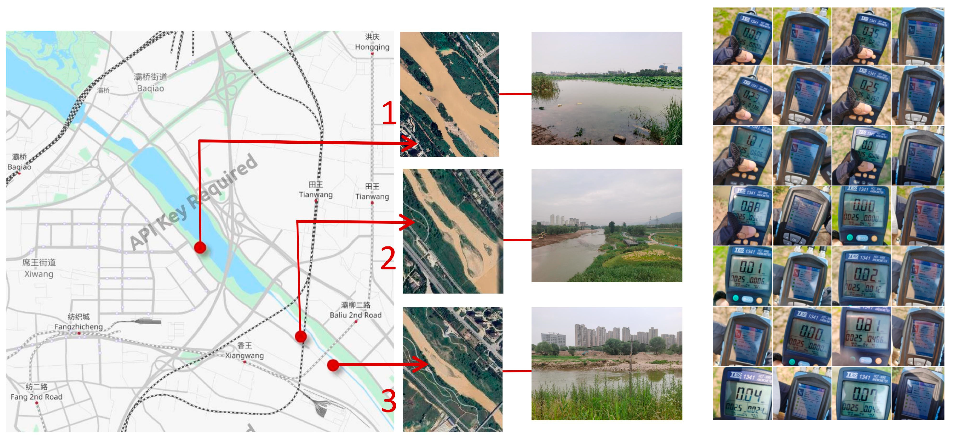
2.1. Study Area
2.2. Field Measurement
2.3. Numerical Simulation
2.3.1. Model Setup
2.3.2. Ideal Scenarios
2.3.3. Outdoor Thermal Comfort
2.4. Verification Analysis
3. Results
3.1. ENVI-Met Verification
3.2. Impact of Landscape Configuration on the Thermal Environment
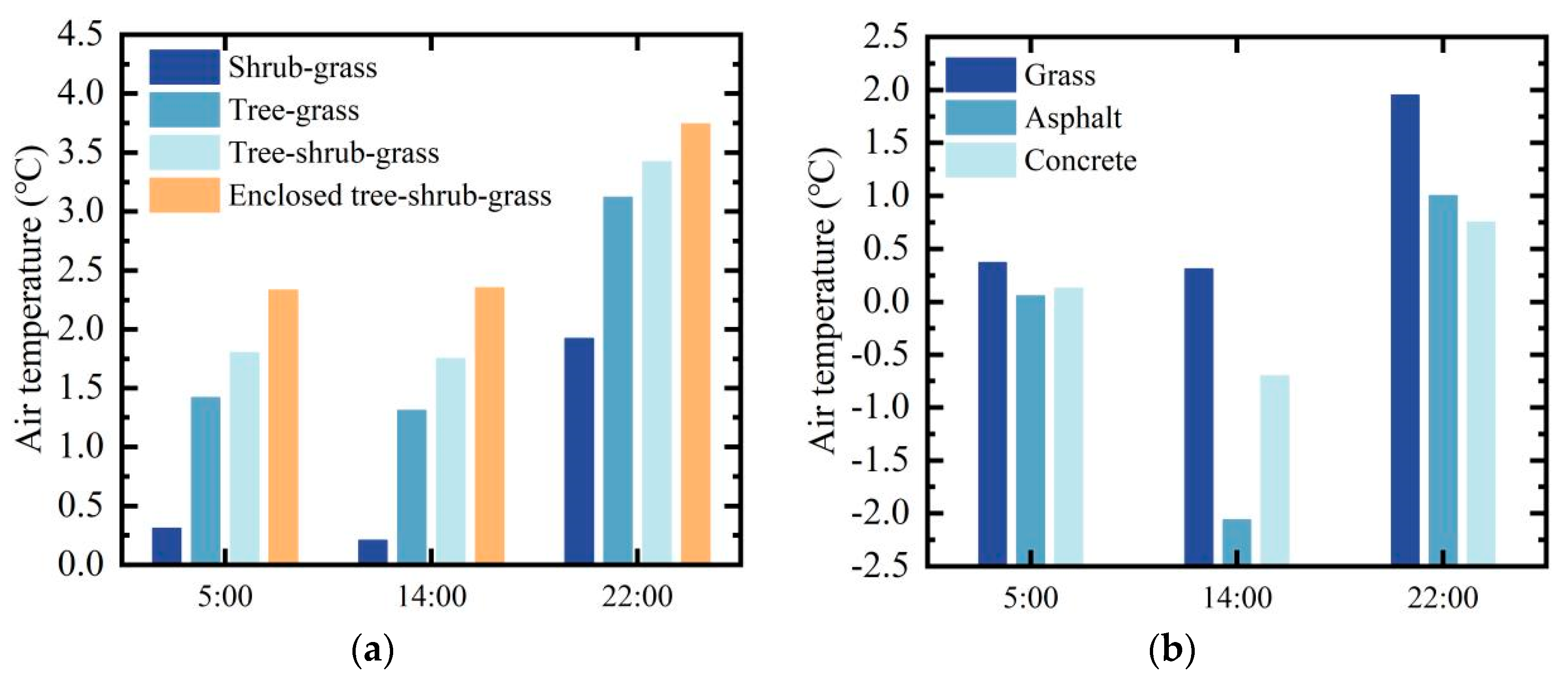
3.2.1. Relationship Between Landscape and the Thermal Environment on River Width of 350 m
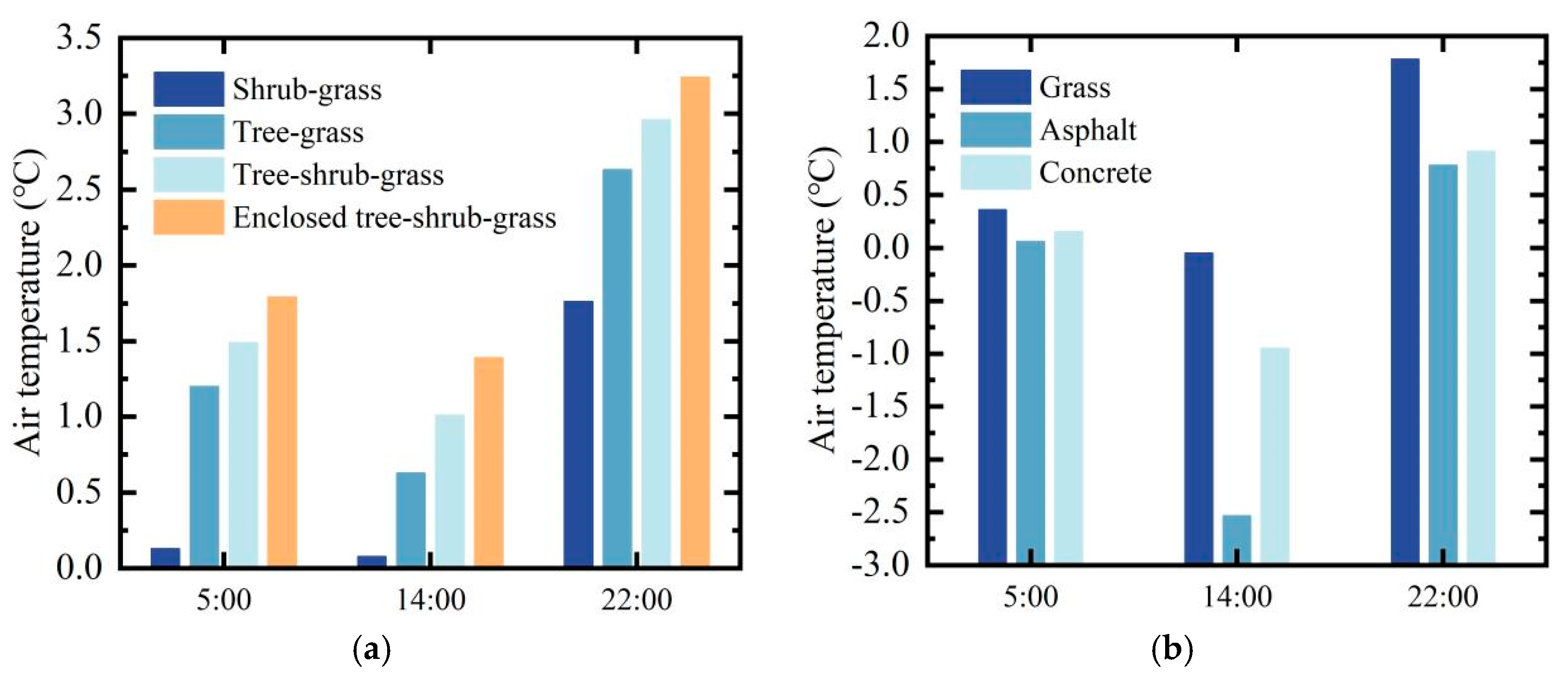
3.2.2. Relationship Between Landscape and the Thermal Environment on River Width of 40 m
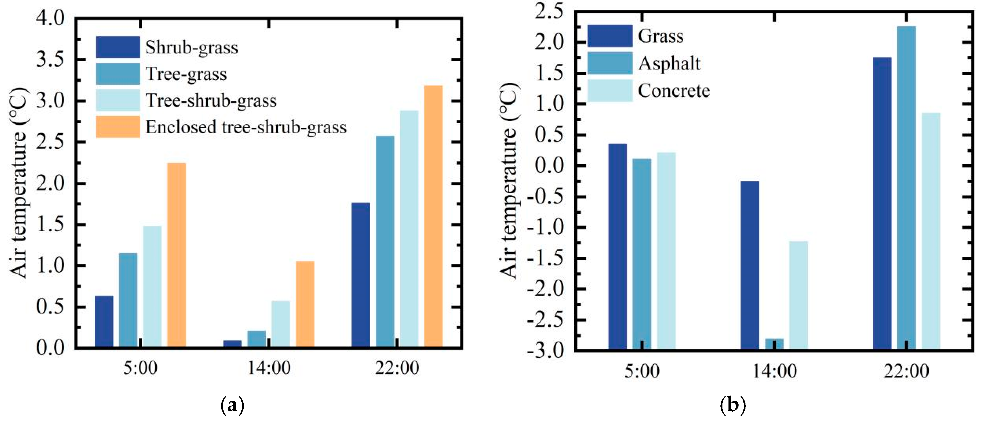
3.2.3. Relationship Between Landscape and the Thermal Environment on River Width of 8 m
3.3. Human Thermal Comfort
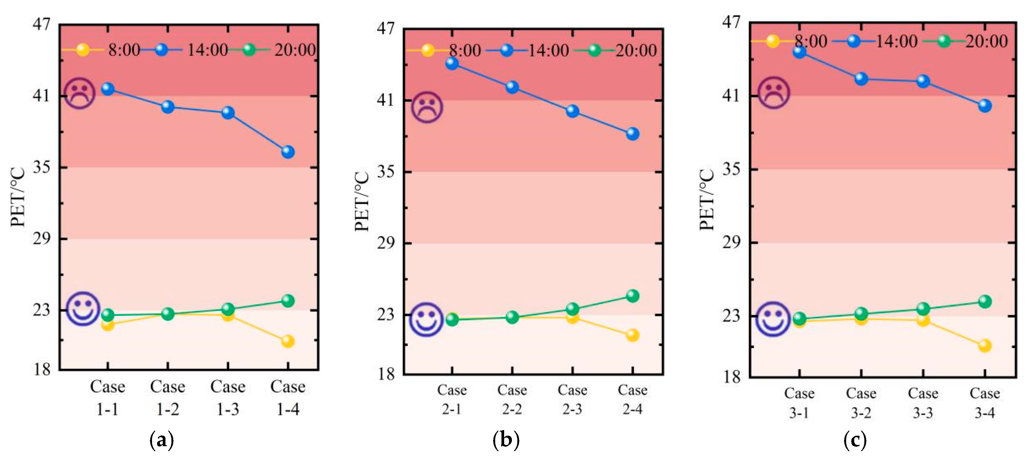
3.3.1. Vegetation Configuration
3.3.2. Underlying Surface
4. Discussion
4.1. Thermal Environment and River-Width
4.2. Thermal Environment and Plant Configurations
4.3. Thermal Environment and Underlying Surface
4.4. Limitations and Future Directions
5. Conclusions
- (1)
- ENVI-met reliability in predicting the local thermal environment of riverside landscape zones is confirmed, with maximum RMSE and d values of 1.10 °C and 0.98, respectively, within an acceptable error range.
- (2)
- Wider rivers show more significant cooling effects. The enclosed tree–shrub–grass configuration is optimal for enhancing riverside thermal environments, with grass being the most effective underlying surface, especially for nighttime cooling, providing a theoretical basis for riverside landscape planning.
- (3)
- PET results indicate that enclosed tree–shrub–grass spaces offer the highest comfort in riverside zones during morning and midday, while shrub–grass areas are more suitable at night, which offers spatial guidance for riverside residents.
Author Contributions
Funding
Data Availability Statement
Conflicts of Interest
References
- Xin, K.; Zhao, J.; Li, Z.; Yang, Y.; Wang, T.; Gao, W. Providing support for urban planning through investigating the cooling influence of park in Northern China: A case study of Xi’an. Urban Clim. 2024, 58, 102221. [Google Scholar] [CrossRef]
- Liang, Z.; Huang, J.; Wang, Y.; Wei, F.; Wu, S.; Jiang, H.; Zhang, X.; Li, S. The mediating effect of air pollution in the impacts of urban form on nighttime urban heat island intensity. Sustain. Cities Soc. 2021, 74, 102985. [Google Scholar] [CrossRef]
- Massetti, L.; Petralli, M.; Brandani, G.; Napoli, M.; Ferrini, F.; Fini, A.; Pearlmutter, D.; Orlandini, S.; Giuntoli, A. Modelling the effect of urban design on thermal comfort and air quality: The SMARTUrban Project. Build. Simul. 2019, 12, 169–175. [Google Scholar] [CrossRef]
- Yang, S.; Wang, L.; Stathopoulos, T.; Marey, A.M. Urban microclimate and its impact on built environment—A review. Build. Environ. 2023, 283, 110334. [Google Scholar] [CrossRef]
- Habibi, A.; Kahe, N. Evaluating the Role of Green Infrastructure in Microclimate and Building Energy Efficiency. Buildings 2024, 14, 825. [Google Scholar] [CrossRef]
- Wang, X.; Fang, Y.; Cai, W.; Ding, C.; Xie, Y. Heating demand with heterogeneity in residential households in the hot summer and cold winter climate zone in China—A quantile regression approach. Energy 2022, 247, 123462. [Google Scholar] [CrossRef]
- Hao, T.; Zhao, Q.; Huang, J. Optimization of tree locations to reduce human heat stress in an urban park. Urban For. Urban Green. 2023, 86, 128017. [Google Scholar] [CrossRef]
- Jiang, Y.; Li, C.; Li, X.; Li, X.; Song, T.; Liu, Y. Exploring the adaptive spatial patterns and impact factors for the cooling effect of park green spaces in riverfront area. Urban Clim. 2024, 55, 101900. [Google Scholar] [CrossRef]
- Sun, B.; Zhang, H.; Zhao, L.; Qu, K.; Liu, W.; Zhuang, Z.; Ye, H. Microclimate Optimization of School Campus Landscape Based on Comfort Assessment. Buildings 2022, 12, 1375. [Google Scholar] [CrossRef]
- Xiao, J.; Yuizono, T.; Li, R. Synergistic Landscape Design Strategies to Renew Thermal Environment: A Case Study of a Cfa-Climate Urban Community in Central Komatsu City, Japan. Sustainability 2024, 16, 5582. [Google Scholar] [CrossRef]
- Srivanit, M.; Hokao, K. Evaluating the cooling effects of greening for improving the outdoor thermal environment at an institutional campus in the summer. Build. Environ. 2013, 66, 158–172. [Google Scholar] [CrossRef]
- Gal, C.V.Z. Revisiting the Urban Block in the Light of Climate Change a Case Study of Budapest. Ph.D. Thesis, Illinois Institute of Technology, Chicago, IL, USA, 2014. [Google Scholar]
- Moss, J.L.; Doick, K.J.; Smith, S.; Shahrestani, M. Influence of evaporative cooling by urban forests on cooling demand in cities. Urban For. Urban Green. 2019, 37, 65–73. [Google Scholar] [CrossRef]
- Gao, Z.; Zaitchik, B.F.; Hou, Y.; Chen, W. Toward park design optimization to mitigate the urban heat Island: Assessment of the cooling effect in five US cities. Sustain. Cities Soc. 2022, 81, 103870. [Google Scholar] [CrossRef]
- Xiao, Y.; Piao, Y.; Wei, W.; Pan, C.; Lee, D.; Zhao, B. A comprehensive framework of cooling effect-accessibility-urban development to assessing and planning park cooling services. Sustain. Cities Soc. 2023, 98, 104817. [Google Scholar] [CrossRef]
- Dong, J.; Chen, J.; Brosofske, K.D.; Naiman, R.J. Modelling air temperature gradients across managed small streams in western Washington. J. Environ. Manag. 1998, 53, 309–321. [Google Scholar] [CrossRef]
- Hathway, E.A.; Sharples, S. The interaction of rivers and urban form in mitigating the Urban Heat Island effect: A UK case study. Build. Environ. 2012, 58, 14–22. [Google Scholar] [CrossRef]
- Coates, M.J.; Folkard, A.M. The effects of littoral zone vegetation on turbulent mixing in lakes. Ecol. Model. 2009, 220, 2714–2726. [Google Scholar] [CrossRef]
- Yang, J.; Su, J.; Xia, J.; Jin, C.; Li, X.; Ge, Q. The impact of spatial form of urban architecture on the urban thermal environment: A case study of the Zhongshan District, Dalian, China. IEEE J. Sel. Top. Appl. Earth Obs. Remote Sens. 2018, 11, 2709–2716. [Google Scholar] [CrossRef]
- Cilek, M.U.; Cilek, A. Analyses of land surface temperature (LST) variability among local climate zones (LCZs) comparing Landsat-8 and ENVI-met model data. Sustain. Cities Soc. 2021, 69, 102877. [Google Scholar] [CrossRef]
- Liu, S.; Middel, A.; Fang, X.; Wu, R. ENVI-met model performance evaluation for courtyard simulations in hot-humid climates. Urban Clim. 2024, 55, 101909. [Google Scholar] [CrossRef]
- Liu, Z.; Cheng, K.Y.; Sinsel, T.; Simon, H.; Jim, C.Y.; Morakinyo, T.E.; He, Y.; Yin, S.; Ouyang, W.; Shi, Y.; et al. Modeling microclimatic effects of trees and green roofs/façades in ENVI-met: Sensitivity tests and proposed model library. Build. Environ. 2023, 244, 110759. [Google Scholar] [CrossRef]
- Du, M.; Hong, B.; Gu, C.J.; Li, Y.C.; Wang, Y.Y. Multiple effects of visual-acoustic-thermal perceptions on the overall comfort of elderly adults in residential outdoor environments. Energy Build. 2023, 283, 112813. [Google Scholar] [CrossRef]
- Zhang, T.; Hong, B.; Su, X.J.; Li, Y.J.; Song, L. Effects of tree seasonal characteristics on thermal-visual perception and thermal comfort. Build. Environ. 2022, 212, 108793. [Google Scholar] [CrossRef]
- Qin, H.Q.; Hong, B.; Huang, B.Z.; Cui, X.; Zhang, T. How dynamic growth of avenue trees affects particulate matter dispersion: CFD simulations in street canyons. Sustain. Cities Soc. 2020, 61, 102331. [Google Scholar] [CrossRef]
- Han, Q.; Nan, X.; Wang, H.; Hu, Y.; Bao, Z.; Yan, H. Optimizing the Surrounding Building Configuration to Improve the Cooling Ability of Urban Parks on Surrounding Neighborhoods. Atmosphere 2023, 14, 914. [Google Scholar] [CrossRef]
- Kim, E.J.; Lee, D.H.; Kang, Y. Explorations on cooling effect of small urban linear park design in low-rise, high-density district: The case of Gyeongui line forest park in Seoul. Urban For. Urban Green. 2024, 100, 128461. [Google Scholar] [CrossRef]
- Zhang, J.; Li, Z.; Hu, D. Effects of urban morphology on thermal comfort at the micro-scale. Sustain. Cities Soc. 2022, 86, 104150. [Google Scholar] [CrossRef]
- Zhang, J.; Li, Z.; Wei, Y.; Hu, D. The impact of the building morphology on microclimate and thermal comfort—A case study in Beijing. Build. Environ. 2022, 223, 109469. [Google Scholar] [CrossRef]
- Xi, T.Y.; Li, Q.; Mochida, A.; Meng, Q.L. Study on the outdoor thermal environment and thermal comfort around campus clusters in subtropical urban areas. Build. Environ. 2012, 52, 162–170. [Google Scholar] [CrossRef]
- Feng, W.; Jing, W.; Zhen, M.; Zhang, J.; Luo, W.; Qin, Z. The difference in thermal comfort between southern and northern Chinese living in the Xi’an cold climate region. Environ. Sci. Pollut. Res. 2023, 30, 48062–48077. [Google Scholar] [CrossRef]
- Xu, M.; Hong, B.; Jiang, R.; An, L.; Zhang, T. Outdoor thermal comfort of shaded spaces in an urban park in the cold region of China. Build. Environ. 2019, 155, 408–420. [Google Scholar] [CrossRef]
- Zheng, W.; Shao, T.; Lin, Y.; Wang, Y.; Dong, C.; Liu, J. A field study on seasonal adaptive thermal comfort of the elderly in nursing homes in Xi’an, China. Build. Environ. 2022, 208, 108623. [Google Scholar] [CrossRef]
- Xin, K.; Zhao, J.Y.; Ma, X.; Han, L.; Liu, Y.Y.; Zhang, J.X.; Gao, Y.J. Effect of urban underlying surface on PM2.5 vertical distribution based on UAV in Xi’an, China. Environ. Monit. Assess. 2021, 193, 312. [Google Scholar] [CrossRef] [PubMed]
- Xin, K.; Zhao, J.; Wang, T.; Gao, W.; Zhang, Q. Architectural Simulations on Spatio-Temporal Changes of Settlement Outdoor Thermal Environment in Guanzhong Area, China. Buildings 2022, 12, 345. [Google Scholar] [CrossRef]
- Ouyang, W.; Sinsel, T.; Simon, H.; Morakinyo, T.E.; Liu, H.; Ng, E. Evaluating the thermal-radiative performance of ENVI-met model for green infrastructure typologies: Experience from a subtropical climate. Build. Environ. 2022, 207, 108427. [Google Scholar] [CrossRef]
- Wang, T.H.; Liu, Y.F.; Wang, D.J.; Gao, W.J. Experimental evaluation on asymmetrical thermal sensation in modular radiant heating system. Build. Environ. 2022, 222, 109433. [Google Scholar] [CrossRef]
- Hegazy, I.R.; Qurnfulah, E.M. Thermal comfort of urban spaces using simulation tools exploring street orientation influence of on the outdoor thermal comfort: A case study of Jeddah, Saudi Arabia. Int. J. Low-Carbon Technol. 2020, 15, 594–606. [Google Scholar] [CrossRef]
- Zhang, Y.; Liu, J.; Zheng, Z.; Fang, Z.; Zhang, X.; Gao, Y.; Xie, Y. Analysis of thermal comfort during movement in a semi-open transition space. Energy Build. 2020, 225, 110312. [Google Scholar] [CrossRef]
- Elnabawi, M.H.; Hamza, N. Outdoor Thermal Comfort: Coupling Microclimatic Parameters with Subjective Thermal Assessment to Design Urban Performative Spaces. Buildings 2020, 10, 238. [Google Scholar] [CrossRef]
- Wai, K.-M.; Yuan, C.; Lai, A.; Yu, P.K.N. Relationship between pedestrian-level outdoor thermal comfort and building morphology in a high-density city. Sci. Total Environ. 2020, 708, 134516. [Google Scholar] [CrossRef]
- Vasilikou, C.; Nikolopoulou, M. Outdoor thermal comfort for pedestrians in movement: Thermal walks in complex urban morphology. Int. J. Biometeorol. 2020, 64, 277–291. [Google Scholar] [CrossRef] [PubMed]
- Fahed, J.; Kinab, E.; Ginestet, S.; Adolphe, L. Impact of urban heat island mitigation measures on microclimate and pedestrian comfort in a dense urban district of Lebanon. Sustain. Cities Soc. 2020, 61, 102375. [Google Scholar] [CrossRef]
- Huang, B.Z.; Hong, B.; Tian, Y.; Yuan, T.T.; Su, M.F. Outdoor thermal benchmarks and thermal safety for children: A study in China’s cold region. Sci. Total Environ. 2021, 787, 147603. [Google Scholar] [CrossRef]
- Mi, J.Y.; Hong, B.; Zhang, T.; Huang, B.Z.; Niu, J.Q. Outdoor thermal benchmarks and their application to climate-responsive designs of residential open spaces in a cold region of China. Build. Environ. 2020, 169, 106592. [Google Scholar] [CrossRef]
- Jeong, C.W.; In, Y. A Study on the Observation of an Urban Climatic Distribution in Pohang City on Summer. Archit. Inst. Korea Plan. Des. 2003, 19, 193–199. [Google Scholar]
- Zhou, Y.; Lu, Y.; Zhou, X.; An, J.; Yan, D. Numerical study on the coupling effect of river attributes and riverside building forms on the urban microclimate: A case study in Nanjing, China. Sustain. Cities Soc. 2024, 107, 105459. [Google Scholar] [CrossRef]
- Qi, X.J.; Zhao, X.; Fu, B.; Xu, L.J.; Yu, H.B.; Tao, S.Y. Numerical Study on the Influence of Rivers on the Urban Microclimate: A Case Study in Chengdu, China. Water 2023, 15, 1408. [Google Scholar] [CrossRef]
- Liu, L.; Wu, J.; Liang, Z.; Gao, J.; Hang, J.; Liu, J.; Liu, L. Spatio-temporal analysis of local thermal environment in waterfront blocks along the both sides of pearl river in Guangzhou, China. Case Stud. Therm. Eng. 2024, 53, 103875. [Google Scholar] [CrossRef]
- Wang, H.; Chen, C. Quantifying the contributions of urban spatial morphology on the river cold island effect: Taking Changsha, China, as an example. Sustain. Cities Soc. 2025, 122, 106256. [Google Scholar] [CrossRef]
- Jiang, L.; Liu, S.; Liu, L.; Liu, C. Revealing the spatiotemporal characteristics and drivers of the block-scale thermal environment near a large river: Evidences from Shanghai, China. Build. Environ. 2022, 226, 109728. [Google Scholar] [CrossRef]
- Jiang, L.; Du, S.S.; Liu, S.; Dong, Y.X.; Yang, Y. Effects of Morphological Factors on Thermal Environment and Thermal Comfort in Riverside Open Spaces of Shanghai, China. Land 2025, 14, 433. [Google Scholar] [CrossRef]
- Deng, Q.L.; Zhou, Z.; Li, C.C.; Yang, G. Influence of a railway station and the Yangtze River on the local urban thermal environment of a subtropical city. J. Asian Archit. Build. Eng. 2022, 21, 589–604. [Google Scholar] [CrossRef]
- Feng, X.G.; Li, M.; Zhou, Z.H.; Li, F.X.; Wang, Y. Quantifying the cooling effect of river and its surrounding land use on local land surface temperature: A case study of Bahe River in Xi’an, China. Egypt. J. Remote Sens. Space Sci. 2023, 26, 975–988. [Google Scholar] [CrossRef]
- Chen, J.K.; Zhan, W.F.; Jin, S.G.; Han, W.Q.; Du, P.J.; Xia, J.S.; Lai, J.M.; Li, J.F.; Liu, Z.H.; Li, L.; et al. Separate and combined impacts of building and tree on urban thermal environment from two- and three-dimensional perspectives. Build. Environ. 2021, 194, 107650. [Google Scholar] [CrossRef]
- Xiao, J.; Yuizono, T. Climate-adaptive landscape design: Microclimate and thermal comfort regulation of station square in the Hokuriku Region, Japan. Build. Environ. 2022, 212, 108813. [Google Scholar] [CrossRef]
- Liu, S.; Zhao, J.; Xu, M.F.; Ahmadian, E. Effects of landscape patterns on the summer microclimate and human comfort in urban squares in China. Sustain. Cities Soc. 2021, 73, 103099. [Google Scholar] [CrossRef]
- Morakinyo, T.E.; Kong, L.; Lau, K.K.L.; Yuan, C.; Ng, E. A study on the impact of shadow-cast and tree species on in-canyon and neighborhood’s thermal comfort. Build. Environ. 2017, 115, 1–17. [Google Scholar] [CrossRef]
- Sodoudi, S.; Zhang, H.W.; Chi, X.L.; Müller, F.; Li, H.D. The influence of spatial configuration of green areas on microclimate and thermal comfort. Urban For. Urban Green. 2018, 34, 85–96. [Google Scholar] [CrossRef]
- Chen, J.K.; Jin, S.G.; Du, P.J. Roles of horizontal and vertical tree canopy structure in mitigating daytime and nighttime urban heat island effects. Int. J. Appl. Earth Obs. Geoinf. 2020, 89, 102060. [Google Scholar] [CrossRef]
- Manavvi, S.; Milosevic, D. Chasing cool: Unveiling the influence of green-blue features on outdoor thermal environment in Roorkee (India). Build. Environ. 2025, 267, 112238. [Google Scholar] [CrossRef]


| Name | Photograph | Type | Measurement Element | Resolution | Range | Precision |
|---|---|---|---|---|---|---|
| Multifunction tester |  | JT2020 | Air temperature | 0.1 °C | −2–120 °C | ±0.2 °C |
| Air humidity | 0.1% | 0–100% | ±2% | |||
| Relative humidity | 0.1% | 0–100% | ±2% | |||
| Black ball temperature | 0.1 °C | 0–50 °C | ±0.2 °C |
| Type | Parameter | Settings |
|---|---|---|
| Location | City | Xi’an |
| Coordinate | 34°32′ N 108°55′ E | |
| Boundary conditions | Turbulence model | Standard TKE model [1] |
| Total simulation time | 24 h | |
| Simulation time | Output interval | 60 min |
| Simulation start time | 5:00 |
| Model Parameter Setting | |||
| River width | 350 m | 40 m | 8 m |
| Number of grids | 150 × 150 | 100 × 100 | 100 × 100 |
| Horizontal resolution | 2 m × 2 m | 2 m × 2 m | 2 m × 2 m |
| Vertical resolution | 1 m × 30 m | 1 m × 30 m | 1 m × 30 m |
| Simulation region | 300 m × 300 m × 5 m | 200 m × 200 m × 5 m | 200 m × 200 m × 5 m |
| Plant configuration ENVI-met data parameter table | |||
| Plant name | Database ID | ||
| Grass | [LG] Luzerne 18 cm | ||
| Shrub | [S1] Scrub 1 m | ||
| Tree | [L1] Privet | ||
| Water | [WW] Deep water | ||
| Underlying surface ENVI-met data parameter table | |||
| Name | Database ID | ||
| Grass | [G1] Grass 10 cm | ||
| Asphalt | [ST] Asphalt | ||
| Concrete | [PP] Pavement (concrete) | ||
| Water | [WW] Deep water | ||
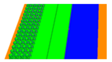
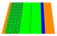
| Different plant configurations | |||
| river width of 350 m | river width of 40 m | river width of 8 m | |
 |  |  | |
| CASE 1-1 Shrub–grass (1:1) | CASE 2-1 Shrub–grass (1:1) | CASE 3-1 Shrub–grass (1:1) | |
 |  | 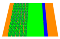 | |
| CASE 1-2 Tree–grass (1:1) | CASE 2-2 Tree–grass (1:1) | CASE 3-2 Tree–grass (1:1) | |
 |  |  | |
| CASE 1-3 Tree–shrub–grass (1:1:1) | CASE 2-3 Tree–shrub–grass (1:1:1) | CASE 3-3 Tree–shrub–grass (1:1:1) | |
 |  | 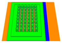 | |
| CASE 1-4 Enclosed tree–shrub–grass (1:1:1) | CASE 2-4 Enclosed tree–shrub–grass (1:1:1) | CASE 3-4 Enclosed tree-–shrub–grass (1:1:1) | |
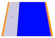
| Different underlying surfaces | |||
| river width of 350 m | river width of 40 m | river width of 8 m | |
 |  |  | |
| CASE 1-5 Grass | CASE 2-5 Grass | CASE 3-5 Grass | |
 |  |  | |
| CASE 1-6 Asphalt | CASE 2-6 Asphalt | CASE 3-6 Asphalt | |
 |  |  | |
| CASE 1-7 Concrete | CASE 2-7 Concrete | CASE 3-7 Concrete | |
| Thermal Sensation | Thermal Stress | PET Range (C) |
|---|---|---|
| Very cold | Extreme cold stress | <13.1 |
| Cold | Strong cold stress | −13.1 to 7.6 |
| Cool | Moderate cold stress | −7.6 to 0.8 |
| Slightly cool | Slight cold stress | −0.8 to 9.8 |
| Neutral | No thermal stress | 9.8 to 30.7 |
| Slightly warm | Slight heat stress | 30.7 to 41.3 |
| Warm | Moderate heat stress | 41.3 to 48.2 |
| Hot | Strong heat stress | 48.2 to 53.6 |
| Very hot | Extreme heat stress | >53.6 |
| Time | Parameter | SITE 1 | SITE 2 | SITE 3 |
|---|---|---|---|---|
| 8:00 | RMSE | 0.22 °C | 0.25 °C | 0.31 °C |
| d | 0.98 | 0.91 | 0.92 | |
| 14:00 | RMSE | 0.81 °C | 0.79 °C | 0.82 °C |
| d | 0.90 | 0.92 | 0.96 | |
| 20:00 | RMSE | 1.10 °C | 1.09 °C | 1.02 °C |
| d | 0.86 | 0.87 | 0.82 |
Disclaimer/Publisher’s Note: The statements, opinions and data contained in all publications are solely those of the individual author(s) and contributor(s) and not of MDPI and/or the editor(s). MDPI and/or the editor(s) disclaim responsibility for any injury to people or property resulting from any ideas, methods, instructions or products referred to in the content. |
© 2025 by the authors. Licensee MDPI, Basel, Switzerland. This article is an open access article distributed under the terms and conditions of the Creative Commons Attribution (CC BY) license (https://creativecommons.org/licenses/by/4.0/).
Share and Cite
Li, Z.; Zhao, J.; Zhang, L.; Xia, B.; Wang, T.; Lu, Y. How Compositions of Landscape Elements Affect Outdoor Thermal Environments: Quantitative Study Along the Urban Riverside. Land 2025, 14, 687. https://doi.org/10.3390/land14040687
Li Z, Zhao J, Zhang L, Xia B, Wang T, Lu Y. How Compositions of Landscape Elements Affect Outdoor Thermal Environments: Quantitative Study Along the Urban Riverside. Land. 2025; 14(4):687. https://doi.org/10.3390/land14040687
Chicago/Turabian StyleLi, Zhaoxin, Jingyuan Zhao, Linrui Zhang, Bo Xia, Tianhui Wang, and Ye Lu. 2025. "How Compositions of Landscape Elements Affect Outdoor Thermal Environments: Quantitative Study Along the Urban Riverside" Land 14, no. 4: 687. https://doi.org/10.3390/land14040687
APA StyleLi, Z., Zhao, J., Zhang, L., Xia, B., Wang, T., & Lu, Y. (2025). How Compositions of Landscape Elements Affect Outdoor Thermal Environments: Quantitative Study Along the Urban Riverside. Land, 14(4), 687. https://doi.org/10.3390/land14040687