Abstract
Urban heat islands (UHIs) constitute one of the most conspicuous anthropogenic impacts on local climates, characterized by elevated land surface temperatures in urban areas compared to surrounding rural regions. This study represents a novel and comprehensive effort to characterize the spectral signature of SUHI through the lens of the two-dimensional (2D) turbulence theory, with a particular focus on identifying energy cascade regimes and their climatic modulation. The theory of two-dimensional (2D) turbulence, first described by Kraichnan and Batchelor, predicts two distinct energy cascade regimes: an inverse energy cascade at larger scales (low wavenumbers) and a direct enstrophy cascade at smaller scales (high wavenumbers). These cascades can be detected and characterized through spatial power spectra analysis, offering a scale-dependent understanding of the SUHI phenomenon. Despite the theoretical appeal, empirical validation of the 2D turbulence hypothesis in urban thermal landscapes remains scarce. This study aims to fill this gap by analyzing the spatial power spectra of land surface temperatures across 14 cities representing diverse climatic zones, capturing varied urban morphologies, structures, and materials. We analyzed multi-decadal LST datasets to compute spatial power spectra across summer and winter seasons, identifying spectral breakpoints that separate large-scale energy retention from small-scale dissipative processes. The findings reveal systematic deviations from classical turbulence scaling laws, with spectral slopes before the breakpoint ranging from ~K−1.6 to ~K−2.7 in winter and ~K−1.5 to ~K−2.4 in summer, while post-breakpoint slopes steepened significantly to ~K−3.5 to ~K−4.6 in winter and ~K−3.3 to ~K−4.3 in summer. These deviations suggest that urban heat turbulence is modulated by anisotropic surface heterogeneities, mesoscale instabilities, and seasonally dependent energy dissipation mechanisms. Notably, desert and Mediterranean climates exhibited the most pronounced small-scale dissipation, whereas oceanic and humid subtropical cities showed more gradual spectral transitions, likely due to differences in moisture availability and convective mixing. These results underscore the necessity of incorporating turbulence theory into urban climate models to better capture the scale-dependent nature of urban heat exchange. The observed spectral breakpoints offer a diagnostic tool for identifying critical scales at which urban heat mitigation strategies—such as green infrastructure, optimized urban ventilation, and reflective materials—can be most effective. Furthermore, our findings highlight the importance of regional climatic context in shaping urban spectral energy distributions, necessitating climate-specific urban design interventions. By advancing our understanding of urban thermal turbulence, this research contributes to the broader discourse on sustainable urban development and resilience in a warming world.
1. Introduction
The rapid urbanization of the 21st century has led to profound transformations in land use and surface energy dynamics [1,2,3], giving rise to the well-documented phenomenon of the Surface Urban Heat Island (SUHI) [4,5,6,7], with a large number of phenomenological studies [8,9,10]. Characterized by elevated surface temperatures in urban areas relative to their rural surroundings [11], SUHI significantly influences the urban boundary layer [12], with cascading effects on energy budgets [13,14], thermal comfort [15], and air quality [16]. Urban areas are complex systems where spatial heterogeneity, anthropogenic activity, and energy exchanges create unique thermal dynamics. Among the emergent phenomena, the SUHI effect has garnered significant scientific attention due to its implications for urban livability [17], energy consumption [18], and public health [19].
Despite extensive research into SUHI and urban boundary layer dynamics, a critical gap remains in understanding how turbulent energy cascades manifest in the complex thermal landscapes of urban environments [20,21]. The recognition of turbulence as a fundamental descriptor of SUHI dynamics shifts the research lens toward understanding the mechanisms of energy distribution and scale-dependent variability. This study ventures into largely uncharted territory, examining SUHI through the framework of turbulence theory—a paradigm that not only complements traditional methodologies but also introduces a dynamic, scale-resolved perspective to urban climatology. Classical turbulence theories, including those of Kolmogorov [22], Batchelor [23], and Kraichnan [24], assume local isotropy and homogeneity within the inertial range at certain scales. Kolmogorov’s theory applies to 3D turbulence, while Batchelor and Kraichnan established the dual cascade framework in 2D turbulence, with energy cascading to larger scales and enstrophy to smaller scales, allowing for anisotropic deviations depending on external forcing and boundary conditions. Urban climates exhibit complex, multi-scale turbulence characteristics influenced by both natural atmospheric processes and modifications due to urbanization. A fundamental question in urban climatology and fluid dynamics concerns how energy is transferred across scales in urban boundary layers, particularly how urban morphology alters classical turbulence theory predictions. Observational studies suggest that urban environments modify this idealized scaling behavior due to heterogeneity in building geometry, land cover, and anthropogenic heat sources. This has been acknowledged by meteorological observational studies, where turbulence spectra and co-spectra have been employed to analyze anisotropy within the urban boundary layer, revealing significant directional dependencies in energy distribution and turbulence structure [25,26]. Spectral analysis has been instrumental in identifying variations in turbulent kinetic energy and heat flux across urban terrains, where distinct anisotropic characteristics emerge due to surface heterogeneities such as urban canopies and thermally contrasting materials [27,28]. For instance, an analysis of turbulence spectra and co-spectra derived from extensive eddy-covariance and other meteorological measurements has highlighted deviations from classical spectral characteristics in urban settings [25,29,30]. These deviations indicate that urban surface roughness and thermal inhomogeneities play a critical role in shaping the distribution of turbulent energy, often leading to an anisotropic structure that differs from the assumptions of classical homogeneous turbulence. Studies have consistently shown that wind turbulence spectra in urban settings differ from those observed in rural environments, and co-spectral analysis of momentum and heat fluxes suggests that these variations are heavily dependent on the local urban morphology and thermal surface properties [11,31,32]. It has also been demonstrated that surface-layer turbulence is directly linked to temperature fluctuations, with surface-temperature structures evolving dynamically as imprints of turbulent coherent structures [33]. These findings further highlight the need to investigate temperature-driven turbulence in urban environments, where additional surface heterogeneities further modulate energy distribution and spectral scaling. Studies using large-eddy simulations (LES) and observational data have consistently demonstrated that urban turbulence deviates from classical homogeneous and isotropic turbulence theories due to the complex interactions between buildings, streets, and atmospheric flow [34,35,36,37]. Furthermore, research has acknowledged the effects of thermally inhomogeneous surfaces in the scaling of turbulent flux co-spectra, showing that temperature fluctuations and associated heat fluxes introduce additional complexity into the turbulent energy transfer process [38,39]. These findings suggest that deviations from classical turbulence theory are not solely a result of mechanical influences but are also driven by urban-induced thermal gradients that modify the spectral characteristics of both velocity and temperature fields [40]. However, most of these studies focus on momentum-based turbulence in wind fields, while temperature-driven turbulence remains largely unexplored in urban environments. While the surface energy balance approach has been extensively applied to urban heat islands [41,42,43,44], these studies primarily quantify sensible and latent heat fluxes at the bulk scale. They do not systematically examine how small-scale turbulent structures mediate spectral energy transfer in temperature fields or how urban form alters these energy cascades. Several studies have investigated turbulence anisotropy and coherent structures in urban areas, demonstrating how built environments alter turbulence characteristics [45,46,47]. However, these studies primarily focus on microscale turbulence structures and do not establish direct connections between spectral energy transfers and large-scale urban heat island (UHI) effects. While anisotropy in urban turbulence has been studied through spectral decomposition, the direct impact of temperature fluctuations on energy cascades and heat flux variability in urban climate dynamics remains underexplored.
Despite these insights, a systematic comparison of spectral slopes over time across multiple climatic zones has yet to be conducted. Urban areas with varying thermal characteristics may show distinct turbulence spectra and co-spectra, impacting energy transfer mechanisms governing urban heat island intensity and atmospheric stability. This study fills this gap by quantifying spectral slope variations across cities in diverse climates, revealing whether deviations are climate-dependent and consistent across urban forms and materials. Integrating a spectral analysis of temperature fields with turbulence theory, we provide a framework for understanding the chaotic, nonlinear nature of urban climate dynamics. Emphasizing temperature-driven turbulence, this research deepens the understanding of how urban forms, materials, and climate interact to modulate energy transfer. Using a spatial power spectral analysis of remotely sensed thermal data (e.g., Landsat, ASTER, ECOSTRESS, MODIS), we captured energy distributions and thus can offer insights into urban thermal processes and the spatial distribution of surface temperatures. This enables an analysis of SUHI spectral signatures and deviations from classical turbulence theory, bridging the theoretical divide and informing urban climate mitigation. By examining cities across five climatic zones, we provide a comparative perspective on turbulent SUHI dynamics and seasonal variations, offering actionable insights into energy retention, dissipation, and heat mitigation strategies. Our research advances urban spectral dynamics, proposing a climate-specific framework for urban energy dissipation modeling and sustainable planning.
1.1. General Framework
1.1.1. Energy Cascades and Thermal Dynamics in Urban Environments
Turbulence describes the irregular and chaotic variations of energy distributions across spatial scales [48]. In urban landscapes, turbulence can be caused by a combination of natural processes (e.g., wind circulation, heat diffusion) and human activity (e.g., transportation, industrial emissions) [49,50]. Thermal turbulence, as measured by LST variance, represents the heterogeneity of thermal characteristics in urban environments. This physical phenomenon is caused by changes in the heat capacity, albedo, and radiative qualities of urban materials (for example, concrete, vegetation, and water bodies) [51,52,53]. Turbulence impacts heat and moisture transfer, hence underlying processes that contribute to the establishment of urban microclimates. It emerges from the complex interplay of urban morphology, material properties, and atmospheric processes, characterized by energy cascades, anisotropy, and heterogeneity. Energy cascade refers to the transfer of energy between different spatial scales, where large-scale fluctuations transfer energy to smaller scales (forward cascade) or small-scale fluctuations contribute to larger-scale patterns (inverse cascade). To quantify these dynamics, energy is conceptualized as the magnitude of thermal variability observed in LSTs, reflecting the intensity of temperature fluctuations across scales, where energy (E) at a given spatial scale is defined as the contribution of variance:
where Ti is the LSTs value at pixel i, is the mean LST, and N is the total number of pixels. This quantification of energy as a function of thermal variability provides a robust framework for analyzing urban turbulence. The spectral analysis of energy distributions across scales reveals how thermal fluctuations are distributed spatially and how they interact with the underlying urban structure. Larger-scale fluctuations, often associated with macro-level urban features such as districts or neighborhoods, dominate the inverse energy cascade regime, where energy flows from smaller to larger scales. Conversely, smaller-scale fluctuations, tied to micro-level features like individual buildings, green spaces, or street canyons, characterize the direct enstrophy cascade, where energy dissipates from larger to smaller scales [54]. In urban LST fields, thermal gradients, surface heterogeneity, and mesoscale processes drive energy transfer and mixing [55]. Energy production occurs at large scales due to solar radiation, urban heat island effects, and anthropogenic heat fluxes, with urban structures and land-use patterns acting as anisotropic forcing mechanisms [56]. Energy transfer within these fields is driven by spatial temperature gradients and thermal diffusion, corresponding to neighborhood-level heat redistribution influenced by vegetation, building density, and material thermal properties [57,58]. At smaller scales, energy dissipation occurs through radiative cooling, conduction, and small-scale atmospheric mixing, dominated by surface roughness and microclimates [59,60,61]. The forward cascade in urban LST fields refers to energy transfer from larger scales (regional temperature gradients or UHI effects) to smaller scales (localized microclimates). This process occurs under three primary conditions: (1) strong thermal gradients generated by solar radiation between different urban surfaces (buildings, roads, vegetation, and water bodies), (2) the UHI effect, where regional-scale temperature differences cascade to smaller scales, and (3) medium-scale heat diffusion between hot surfaces (e.g., asphalt) and cooler areas (e.g., vegetation or water), amplified by local wind patterns and turbulent eddies. The inverse cascade involves smaller-scale energy (arising from microclimates) being transferred to larger scales, reinforcing broader temperature patterns. This occurs through (1) destabilization of the surrounding air mass due to small-scale thermal differences, (2) upward thermal plumes from heated urban surfaces contributing to convection cells, and (3) urban planning features such as tall buildings or expansive parking lots that redirect heat to larger atmospheric structures, intensifying the UHI effect.
1.1.2. Eddies and Instabilities in Urban LST Fields
Eddies in urban LST fields represent vortex-like movements driven by thermal gradients, surface roughness, and wind interactions. These eddies facilitate heat redistribution, impacting the spatial and temporal dynamics of LST. They form due to differential heating between urban surfaces (e.g., asphalt, buildings) and cooler regions, generating vertical and horizontal air circulation. Vertical transport occurs as warm air rises from heated surfaces, while horizontal mixing circulates air between hotter and cooler regions, smoothing temperature variations. The resulting energy cascade transfers heat across multiple spatial scales, reinforcing localized thermal hotspots and microclimates, which exacerbate the UHI effect. Eddies contribute to fluctuating temporal LST patterns, with their dynamics further amplifying urban warming via interaction with the UHI feedback loop.
Thermal instabilities emerge as disturbances in the LST distribution driven by uneven surface heating and interactions between the land and atmosphere. These processes are influenced by urban heterogeneity, such as diverse material properties and geometries. Land-atmosphere coupling amplifies these instabilities, fostering complex energy transfer dynamics that reshape urban heat fields. The interplay between surface processes (e.g., absorption and emission of heat) and atmospheric dynamics (e.g., convection and wind patterns) underscores the significance of feedback mechanisms in urban thermal variability.
1.1.3. Energy Spectrum in LST Fields
The energy-containing range corresponds to large-scale phenomena such as UHIs, influenced by city morphology and land-use patterns. The inertial subrange reflects neighborhood-level gradients and diffusion-dominated energy transfer. Finally, the dissipation range captures fine-scale heterogeneity caused by individual buildings, vegetation, or pavement materials. Strong anisotropy in urban LST fields arises from directional influences like street orientation, building geometries, and vegetation distributions. These elements constrain thermal gradients and energy transfer, with external drivers such as solar radiation and anthropogenic heat further shaping the patterns. In UHIs, mesoscale processes drive regional energy redistribution via large-scale temperature gradients. Furthermore, boundary-layer dynamics between the urban surface and the atmosphere create mesoscale thermal circulations that modulate the LST field and contribute to complex heat dynamics at these intermediate scales. The spatial power spectrum of urban LST fields elucidates the distribution of energy across scales. Peaks at large scales represent UHIs, medium scales highlight neighborhood-level gradients, and small scales capture localized variability. This spectral analysis provides a comprehensive understanding of energy dynamics in urban environments, emphasizing the intricate interplay between large-scale forcings and small-scale processes.
1.1.4. Surface Temperature as a Result of Energy Balance Components
Surface temperature (LST) in urban areas is primarily governed by the surface energy balance model (SEB) [43], expressed as:
where Rn is net radiation, determined by solar and longwave radiation; H is sensible heat flux, representing turbulent heat exchange with the atmosphere; LE is latent heat flux, controlled by evapotranspiration; G is ground heat flux, representing energy storage in urban materials; and QA is anthropogenic heat flux, influenced by human activity (e.g., transportation, industry). Our study focuses on how turbulent energy exchange (H, LE) manifests in the spectral characteristics of LST fields, capturing deviations from classical turbulence theory. The presence of breakpoints in the LST spectra reflects shifts in dominant energy transfer processes, distinguishing large-scale thermal retention from small-scale dissipative mechanisms.
Rn = H + LE + G + QA
The introduction of spectral analysis to urban SUHI studies addresses these gaps, offering a quantitative lens to dissect the intricate interplay of energy transfer mechanisms. The central hypothesis of this study posits the existence of a spectral breakpoint, indicative of a transition between large-scale thermal anomalies and small-scale dissipative processes. By analyzing energy spectra, we can identify critical transition points where energy shifts from large-scale organization to small-scale dissipation—a hallmark of turbulence. These transitions provide insights into the processes governing heat and moisture transport in urban areas, with implications for the understanding of urban energy budgets and boundary layer behavior. Furthermore, the spectral framework enables a robust comparison across diverse urban typologies, facilitating the development of generalized theories that account for climatic and morphological variability. By integrating atmospheric science, urban climatology, and turbulence theory, it presents a new theoretical framework that complements traditional paradigms and emphasizes the role of scale-dependent processes in shaping urban thermal landscapes. The findings contribute to sustainable urban development by revealing the turbulent dynamics of SUHI across different climatic zones.
2. Materials and Methods
2.1. Data Collection and Preprocessing
2.1.1. Selection of Study Areas
This study analyzed the land surface temperature (LST) and urban heat island (UHI) effects for 14 cities located in diverse climatic zones (Figure 1). Cities were selected based on the Köppen–Geiger climate classification [62] to ensure representation across various climatic conditions, including arid, temperate, subtropical, oceanic, desert, and Mediterranean zones. The cities analyzed in this study were Santiago (Chile), Córdoba (Argentina), Chandigarh (India), Skopje (North Macedonia), Tirana (Albania), Madrid (Spain), Paris (France), Tbilisi (Georgia), Ankara (Turkey), Amman (Jordan), Las Vegas (Nevada, USA), Nashville (Tennessee, USA), Wuhan (China), and Belo Horizonte (Brazil). This selection ensures that the study captures a range of urban morphologies, climates, and thermal dynamics. While these cities differ in area, terrain, population density, and economic activity, our study focuses on thermal turbulence and spectral energy transfer, which are largely determined by (a) urban morphology (building density, land cover heterogeneity), (b) surface material properties (albedo, heat capacity, roughness effects), and (c) regional climatic forcing (solar radiation, atmospheric stability, precipitation). These fundamental drivers of urban heat turbulence operate independently of economic and demographic factors, ensuring that our spectral analysis remains physically robust across different urban contexts. Furthermore, previous studies on urban climate turbulence [11,32,41] have demonstrated that the scaling behavior of urban heat transfer follows universal principles, despite variations in socioeconomic characteristics. Additionally, our selection method ensures statistical consistency across climatic zones, reducing the influence of potential outliers. The observed spectral breakpoints and slope deviations were consistent across cities within the same climatic zone, reinforcing the reliability of our conclusions. The systematic differences in spectral characteristics between climatic zones confirm that our findings are climate-dependent rather than city-dependent. By integrating multiple cities within each climate type, we capture a broader and more generalizable understanding of how climate modulates urban thermal turbulence. This selection approach aligns with previous research on urban spectral scaling [28,30], which has demonstrated that fundamental turbulence scaling behaviors persist across different urban environments. Consequently, our results are not biased by individual city characteristics but instead reflect broader climate-driven mechanisms of energy transfer in urban heat island dynamics. By justifying city selection through climatic classification while acknowledging urban morphological differences, we ensure that our study provides a robust framework for understanding climate-specific thermal turbulence across urban environments.
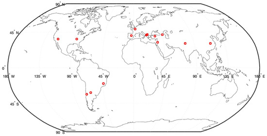
Figure 1.
Spatial distribution of cities/locations under study. The red squares represent the cities/locations under study.
2.1.2. Satellite Image Selection
LST series data were derived from Landsat 5, 8, and 9 imagery, which was originally collected at 100 m and resampled to 30 m with an orbital frequency of 16 days (Figure 2 and Figure 3). The gathered dataset covers a temporal range from the 2000s to the present with the following selection criteria. For each decade, a typical summer and winter day was selected, defining a total sample of six images per city/location of study. Images were selected aiming at minimizing cloud cover. A low cloud cover maximizes data reliability and minimizes errors introduced by cloud contamination and pixel removal by cloud masking. Additionally, Landsat scenes that provide full coverage of the urbanized area, as well as sufficient surrounding space in the scene to include a buffer zone of non-urban pixels for integrating UHI effects and geographic background, were selected, preserving uniformity in the spatial extent across regions. Given the sampling requirements for an appropriate further estimation of the power spectra of cities/locations, we avoided using scare buffering space in the Landsat scene as well as sea/coastal cities.
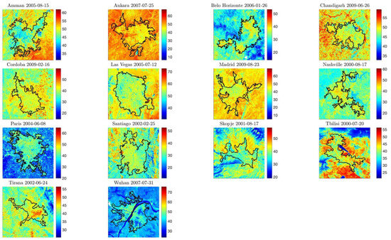
Figure 2.
Sample of land surface temperature images corresponding to Landsat 5 for the summer season of the decadal period of the 2000s. The black shape corresponds to the metropolitan area of each city under study.
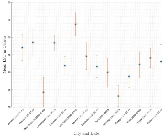
Figure 3.
Mean LST values for the urbanized areas (black shape) of the 14 cities sampled in Figure 2; error bars correspond to standard deviation.
Landsat satellites maintain a synchronous orbit with the sun with a consistent overpass time, ensuring that all images are acquired within a narrow time window around 10:00 AM local solar time. This minimizes potential biases in LST comparisons across cities. As the satellite captures LST during the morning heating phase, before peak urban heating, it provides a stable basis for analyzing spatial energy distributions. While minor variations in overpass time (typically within 30 to 90 min) exist due to orbital and geographic factors, they do not significantly impact spectral comparisons. The methodology focuses on relative energy distributions across spatial scales, making it robust to temporal discrepancies in absolute LST values. By emphasizing urban morphology, surface properties, and climatic influences, rather than diurnal fluctuations, the approach ensures a meaningful spectral analysis across diverse urban environments.
2.1.3. Generation of Square Images for Power Spectrum Estimation
To standardize the analysis and enable power spectrum estimation, this study adopted a structured approach to generate square images of the urbanized areas and their surroundings. For each city/location under study, a bounding box was created based on the shapefile of the urbanized area. To obtain the footprint of urbanized areas, the Global Urban Areas dataset available from Daylight was employed [63], the selection of the urban footprint shapefile was done using QGIS software (v.3.34) [64]. The bounding box was extended outward to the nearest integer dimension, ensuring a square image format. This approach encapsulated the urban core, its periphery, and a buffer zone of non-urban pixels. The resulting square images captured the transition from the urbanized area to its borders and extended into surrounding non-urban pixels. This configuration mimics the radial structure of urban areas and their influence on the surrounding landscape, facilitating comprehensive UHI analysis. The square images ensured uniformity across cities, allowing for consistent spectral and spatial analysis.
2.1.4. Climatic and Geographic Diversity
The selected cities span a wide range of climatic and geographic conditions. By including cities from multiple continents and climate zones, this study provides insights into how urban morphology and climatic conditions influence LST and UHI characteristics. A summary of the selected cities and their corresponding Köppen–Geiger climate classifications is provided in Table 1.

Table 1.
Climatic zones of the locations under study according to Köppen–Geiger classification.
2.1.5. Justification for Methodology
The use of square bounding boxes was crucial to standardizing spatial analysis and facilitating the spectral analysis of urbanized areas. By extending the bounding boxes to include non-urban pixels, the method captures the full extent of the urban thermal signature while providing a buffer for the better characterization of UHI effects. This approach allows for consistent power spectrum estimation and meaningful cross-city comparisons.
2.2. Generating the Power Spectrum from LST Images
The data analysis starts with the generation of the power spectrum from the LST images. The LST data for each location of the study were selected, cloud and snow-maked employing GEE. Afterwards, were downloaded in GeoTIFF format. To ensure the quality of the dataset, the presence of missing values due to the marking process was filled using nearest-neighbor interpolation to minimize the distortion of the Fourier Transform caused by missing values. The codes were written in MATLAB Ver. 2024a [65], although the approach employed was partly inspired by the implementation of the Python (v.3.11.5) statistical analysis package TURBUSTAT [66,67]. The Fourier Transform is computed to shift the image from the spatial domain to the frequency domain. This is performed using the discrete Fourier Transform (DFT) of a 2D signal f(x,y); the following equation transforms spatial data (x,y) into the frequency domain (u,v):
where f(x,y) is the spatial domain representation of the image (intensity at pixel (x,y)); F(u,v) is the frequency domain representation of the image, indicating the amplitude and phase of spatial frequency components. Nx, Ny are the total number of pixels along the x- and y-axes, respectively. The spatial frequency components in the horizontal (x) and vertical (y) directions are represented by u and v. The complex exponential function representing the Fourier basis is represented by . The power spectrum, which measures the strength (magnitude) of the frequency components in the transformed domain, is visualized to study the distribution of frequencies in an image. It is derived as the squared magnitude of the Fourier Transform and can be described as:
where P(u,v) is the squared magnitude, representing the power or energy contained at each frequency (u,v), with u as the frequency in the horizontal direction (e.g., cycles per unit length along x) and v as the frequency in the vertical direction (e.g., cycles per unit length along y). The term ∣F(u,v)∣ corresponds to the magnitude of the Fourier Transform at frequency (u,v), computed as:
This coefficient encodes both the amplitude and phase of the frequency component. The real part of F(u,v), denoted as Re(F(u,v)), corresponds to the contribution of cosine waves to the frequency component, and it can be interpreted as the x-coordinate of the complex number in the complex plane. Conversely, the imaginary part, Im(F(u,v)), represents the contribution of sine waves and is the y-coordinate of the same complex number. Together, these components provide a complete description of the frequency’s behavior within the system. The radial spatial frequency, which is the Euclidean distance from the origin (center of the frequency domain) to the frequency component at (u,v), is represented as:
where the square route is used to compute the radial distance, combining as the normalized frequency component along the x-axis and as the normalized frequency in the y-axis. The radius is used for radial averaging in power spectrum analysis, where frequencies are grouped and averaged by their distance from the center of the frequency domain. To analyze the power spectrum as a function of spatial frequency, the data are binned into intervals based on Scott’s rule for optimal bin width following the equation:
where h is the bin width, σ is the standard deviation, and n is the number of data points. A logarithmic binning strategy is used to better capture the behavior of the power spectrum at lower frequencies. The power spectrum is further averaged within each bin to calculate the radial power spectrum. Invalid bins (empty or missing values) are excluded.
2.3. Detecting the Optimal Breakpoint in a Power Spectrum of a Signal
2.3.1. Breakpoint Identification
The process of detecting the optimal breakpoint in a power spectrum, where distinct scaling behaviors occur, was implemented by minimizing the residual error between data and two-segment linear fits. The code was written in MATLAB [65]. The raw data, consisting of spatial frequency f and power spectrum P, are initially processed to exclude any non-positive and missing values or NaN values. This step ensures that the analysis focuses solely on valid data points. The remaining data are subjected to a log–log transformation, converting the frequency and power values to their base-10 logarithms. This log–log transformation enhances the linearity of power-law distributions, facilitating the identification of different scaling regimes. The breakpoint is identified by testing multiple candidate points within the data. These candidate breakpoints are chosen between the second and penultimate data points to avoid edge effects. For each candidate breakpoint, a two-segment linear fit is applied to the data before and after the candidate point. For the first segment (before the breakpoint), the linear fit is represented as follows:
For the second segment (after the breakpoint), the linear fit is represented as:
where and denote the slopes and b1 and b2 represent the intercepts of the respective fits. The quality of each breakpoint candidate is evaluated by calculating the residual error, defined as the sum of squared differences between the actual and predicted values of power in both segments:
where (i) and (i) are the values predicted by the linear fits of the first and second segments, respectively. The residual error E captures the discrepancy between the observed data and the two linear models. The breakpoint with the minimum residual error is selected as the optimal breakpoint. Once the residual errors for all candidate breakpoints are computed, the optimal breakpoint is chosen as the point that yields the minimum residual error. This breakpoint represents the location where the power spectrum undergoes a significant change in scaling behavior.
2.3.2. Model Fitting and Evaluation
After selecting the optimal breakpoint, two linear models are fitted to the data: one for the segment before the breakpoint and another for the segment after the breakpoint. The goodness of fit for each model is assessed using the coefficient of determination, or R-squared (R2):
where SSres is the residual sum of squares and SStot is the total sum of squares:
where is the mean of the observed power values for the segment. The R-squared values for the first and second segments are calculated separately, reflecting the fit quality of each segment. These metrics quantify the fit quality of each segment and are used to evaluate the performance of the two-segment model. This method allows for the identification of a clear breakpoint in the power spectrum, marking the transition between different scaling regimes, and provides a robust way to characterize the scaling behavior of the data.
A generalized schematic diagram of the methodological workflow describing the different stages in the process of obtaining the spectral slope is proposed below (Figure 4).
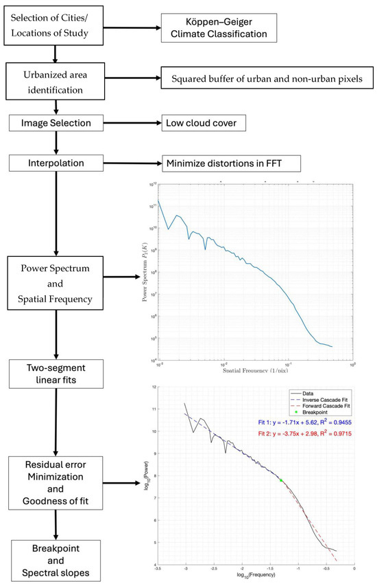
Figure 4.
General scheme of the methodological process performed for obtaining the spectral slopes.
3. Results and Discussion
The results corresponding to the spatial power spectrum for the 14 cities/locations under study, spanning from the 2000s to the present, with two representative spectra (summer and winter) selected per decade (Figure 5) are presented. Each spectrum captures variations in spatial frequency (log10) against the log-transformed power spectrum, revealing the multi-scale thermal structure of UHI phenomena. Each city’s average spectral breakpoint (marked by the dashed line) demarcates the transition from large-scale to small-scale thermal processes, offering a quantitative metric for urban thermal structure. The spectra’s slopes and breakpoints highlight deviations from the classical 2D turbulence hypothesis as proposed by Kraichnan and Batchelor. These deviations are explored quantitatively, providing insight into urban thermal dynamics and their divergence from theoretical expectations. The spectral breakpoints highlight the scale of dominant thermal processes in each city. These values vary across the cities, with Tirana (−1.53) exhibiting the smallest breakpoint (indicating the dominance of finer-scale processes) and Nashville (−1.12) showing the largest (suggesting the dominance of coarser-scale thermal patterns). Cities with breakpoints closer to −1.5 (e.g., Santiago, Wuhan) tend to exhibit sharper gradients in temperature, indicative of heterogeneous urban morphology and material composition. The consistent positioning of spectral curves across decades reflects temporal stability in thermal processes within each city. Seasonal differences between the summer and winter spectra are evident, particularly in cities with pronounced climatic variations (e.g., Belo Horizonte, Paris). Cities with dense, compact urban centers (e.g., Paris, Cordoba) show distinct spectral curves, indicative of strong anisotropy in thermal energy distribution. In contrast, sprawling cities (e.g., Las Vegas, Nashville) display smoother transitions, suggesting more homogeneous energy dynamics. Breakpoints provide a quantifiable measure to compare urban morphologies. For example, Tirana and Santiago, with more negative breakpoints, may exhibit higher thermal heterogeneity, while Nashville and Tbilisi show smoother energy transitions. These variations can be linked to differences in urban planning, green space integration, and building material properties. The gradual convergence or divergence of spectral curves within each city provides insights into the evolving nature of urban heat islands (UHI). For instance, the spectral alignment across decades in Wuhan and Madrid suggests persistent UHI effects. The differences between spectral breakpoints across cities underscore the role of urban geometry and material properties in modulating thermal energy transfer.
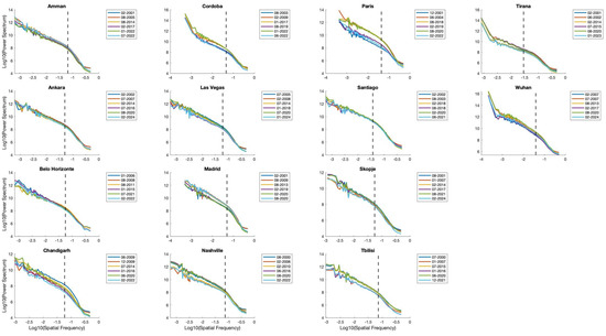
Figure 5.
Spatial power spectrum for the 14 cities/locations under study. One spectrum for summer and one for winter per decade from the 2000s to the present are presented. The black dashed line indicates the optimal spectral breakpoint location obtained by minimizing the residual error method.
The spectral analysis underscores the importance of scale in understanding urban heat dynamics. The breakpoint serves as a critical threshold separating large-scale processes (e.g., solar heating, urban heat islands) from small-scale processes (e.g., vegetation cooling, building heat retention). The variability in spectral curves reflects the interplay of urban morphology, climate, and human activity. These insights are crucial for tailoring urban planning and mitigation strategies to specific cities. The average spectral breakpoint provides a new metric for assessing thermal heterogeneity and urban sustainability, particularly in the context of climate change adaptation.
3.1. Observed Spectral Regimes
The observed energy spectra in urban environments, particularly in UHIs, are influenced by thermal instabilities driven by seasonal variations in surface temperature gradients, urban boundary layer dynamics, and spatial heterogeneities caused by urban morphology. Unlike the theoretical 2D turbulence theory, these instabilities drive energy transfer across scales in a non-uniform and seasonally modulated manner, leading to deviations from the classical forward cascade ~K−5/3 and inverse cascade ~K−3 slope. The spectral analysis reveals distinct deviations from the classical 2D turbulence hypothesis, highlighting transitions at spectral breakpoints that delineate scale-dependent thermal dynamics. The slopes are presented in two regimes: before the spectral breakpoint, with observed slopes across all 14 cities ranging from ~K−1.6 to ~K−2.7 during winter and ~K−1.5 to ~K−2.4 during summer. The median slope values were K−2.13 (summer) and K−1.91 (winter), with interquartile ranges (IQRs) highlighting consistent patterns of variability. Notably, the range of deviations exceeded theoretical expectations (e.g., ~K−5/3 slope for inverse energy cascade), while after the spectral breakpoint, the slopes ranged from ~K−3.5 to ~K−4.6 in winter and ~K−3.3 to ~K−4.3 in summer. The median slope values were K−4.10 (summer) and
K−3.84 (winter), with significant variability reflecting dissipative processes at smaller scales also deviating from the theoretical expected ~K−3. These deviations suggest that the urban thermal environment exhibits a steeper dissipation rate at smaller scales compared to natural turbulence. Seasonal differences further modulate the spectral slopes, with summer exhibiting relatively flatter slopes before the breakpoint compared to winter, indicative of enhanced thermal mixing during warmer months (Figure 6).
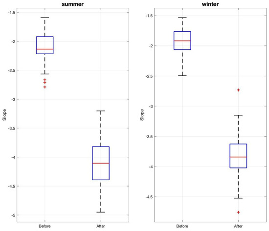
Figure 6.
Seasonal distribution of slopes before and after spectral breakpoint.
Four key mechanisms underly such deviation: First, seasonal surface temperature gradients and their effect on turbulence and energy transfer. The seasonal surface temperature gradients imply that the summer’s higher surface temperatures intensify the vertical and horizontal thermal gradients, enhancing buoyancy-driven turbulence and creating more chaotic and intermittent energy transfer across scales, while winter reduced thermal gradients together with a more stable boundary layer, allowing for longer persistence of the mesoscale structures and smoother energy cascades [68,69]. Second, urban surface heterogeneities derived from urban landscape morphology introduce localized heat sources and sinks (e.g., asphalt, green spaces, and water bodies) that create spatial variability in mixed-layer turbulence [70]. These variations prevent the formation of a uniform energy cascade and instead produce localized energy bottlenecks and intermittent bursts of energy transfer. Third, coherent thermal and aerodynamic mesoscale structures dominate energy transfer. At larger spatial scales, there exist coherent thermal and aerodynamic mesoscale structures (e.g., heat plumes, wake turbulence, and horizontal rolls) that dominate energy transfer [71], aligning more with mixed-layer instability mechanisms than with homogeneous 2D turbulence. Fourth, the seasonal modulation of energy transfer mechanisms across spatial scales. In the energy transfer mechanism across spatial scales during summer, increased vertical mixing disrupts the smooth horizontal energy cascade, introducing anisotropy in the energy transfer, while during winter, the reduced vertical mixing allows for horizontal energy cascades to dominate, possibly aligning more closely with traditional turbulence spectra [72,73]. The spectral characteristics under study comprise seasonal urban boundary layer-mixed instabilities. The summer season enhances the urban boundary layer, with mixed instabilities deviating significantly from K−5/3 steeper spectral slopes after the breakpoint, reflecting increased vertical mixing, buoyancy-driven convection, and wake turbulence, while the winter season stabilizes the boundary layer, partially aligning with the K−5/3 slope at larger scales and less steep slopes after the breakpoint due to horizontal energy cascades and reduced vertical mixing.
3.2. Summer Season: Enhanced Mixed-Layer Instabilities
At small scales during summer, enhanced thermal instabilities dominate the urban boundary layer driven by intense solar radiation, strong surface heating, and the heterogeneity of urban morphology, which results in vertical mixing, buoyancy-driven convection, and wake turbulence around urban structures, influencing the spectral energy distribution across spatial scales. At such small spatial scales, the turbulence becomes highly chaotic, and energy dissipation dominates (e.g., spectral slopes near ~K−4.5 to ~K−5.0 in Amman and Las Vegas). At larger spatial scales, buoyancy-driven convection organizes mesoscale structures, with energy cascading less chaotically (e.g., spectral slopes near ~K−2.0 to ~K−2.4 in Tbilisi). Tall buildings and complex urban geometries also create wake turbulence and shear instabilities as wind flows around obstacles. These wakes interact with thermal plumes, adding mechanical turbulence to the buoyancy-driven turbulence. Wind shear at the building level amplifies localized eddies, further enhancing energy dissipation at smaller scales. Cities with dense high-rise areas (e.g., Santiago, K−4.52 in 2020) show steep spectral slopes at smaller scales due to enhanced turbulence from wake effects and strong surface heating. This leads to two convection regimes. A free convection regime occurs in areas with weak wind speeds and strong heating, where turbulence is dominated by vertical thermal plumes. A forced convection regime happens at a location with moderate-to-high wind speeds, where turbulence is mechanically driven, creating horizontal eddies and interacting with rising heat plumes. In summer, urban boundary layers tend to be turbulent and chaotic at smaller scales, while organized energy structures dominate at larger scales. Enhanced instabilities emerge from the interaction between thermal plumes, wake turbulence, and urban morphology (Table 2).
Table 2.
Seasonal comparison showing contrasts between enhanced instabilities in summer against stabilized layers in winter.
3.3. Winter Season: Stabilized Boundary Layers
During winter, stabilized boundary layers dominate the urban atmosphere, characterized by weaker surface heating, reduced buoyancy-driven convection, and more stratified air masses. These factors suppress vertical mixing and reduce turbulence intensity at smaller scales. At smaller spatial scales, turbulence is less intense, and spectral slopes are less steep (e.g., around ~K−4.0 in Ankara and Santiago). At larger spatial scales, energy transfer aligns more with horizontal advection and mesoscale circulations (e.g., spectral slopes near ~K−1.7 to ~K−2.0 in Ankara). With suppressed vertical mixing, horizontal energy transport becomes the dominant mechanism. Wind-driven advection and large-scale flow patterns play a greater role in distributing energy across the urban boundary layer. Larger-scale mesoscale structures dominate energy cascades, creating smoother spectral transitions between scales. Cities in more stable winter conditions (e.g., Madrid, Ankara) exhibit spectral breakpoints, reflecting the dominance of mesoscale advection and reduced vertical exchange. Urban morphology (e.g., building clusters, narrow streets) still generates localized turbulence pockets through mechanical wind shear and wake effects. The thermal inertia of building materials can create small-scale temperature gradients, generating localized mixing zones. In winter, urban boundary layers are stratified and less turbulent at smaller scales, with horizontal energy transport dominating at larger scales. Energy transfer becomes smoother and more predictable, aligning better with theoretical turbulence models. In colder seasons, smaller-scale turbulence is reduced due to stabilized atmospheric conditions, although residual heterogeneities in urban structures and heat retention from the built environment still generate localized instabilities (Table 2).
In summer, energy cascades transition sharply at the spectral breakpoint, with steep slopes reflecting chaotic turbulence, while in winter, energy cascades are smoother, with energy being more horizontally distributed across mesoscale structures. Urban morphology and local wind patterns interact with these seasonal dynamics, modulating the spectral energy distribution. In both winter and summer, increased energy dissipation and smaller-scale turbulence are shown. At large scales, which correspond to more organized energy cascades and coherent mesoscale structures shown during summer, strong vertical convection and surface heating heterogeneities dominate mesoscale dynamics. This analysis underscores how seasonal atmospheric conditions fundamentally alter turbulence and energy transfer across spatial scales in urban environments.
3.4. Spatial Scale Dependence Across Cities and Seasonal Trends
The spectral slope values also provide key insights into the spatial scale dependence of energy distribution and turbulence in urban boundary layers across seasons. In both summer and winter, the slopes after the spectral breakpoint (steeper negative slopes, e.g., ~K−4.0 to ~K−5.0) indicate increased energy dissipation and smaller-scale turbulence. During summer, cities such as Amman (K−4.95 in 2014) and Las Vegas (K−4.48 in 2020) exhibit more pronounced energy dissipation at smaller scales, likely due to enhanced vertical mixing, buoyancy-driven convection, and wake turbulence around urban structures. During winter, while smaller-scale turbulence is reduced due to stabilized atmospheric conditions, residual heterogeneities in urban structures and heat retention from the built environment still generate localized instabilities (e.g., Santiago, ~K−4.02 in 2018). Larger scales (shallower slopes closer to ~K−1.5 to ~K−2.0) correspond to more organized energy cascades and coherent mesoscale structures. During summer, larger-scale slopes (e.g., ~K−2.0 to ~K−2.4) suggest that strong vertical convection and surface heating heterogeneities dominate mesoscale dynamics (e.g., Tbilisi, ~K−2.46 in 2015), while during winter, the larger-scale energy cascade aligns more closely with theoretical turbulence models, with slopes around ~K−1.7 to ~K−2.0 (e.g., Ankara, ~K−1.7 in 2002). This reflects horizontal energy transport and mesoscale circulation patterns under stable atmospheric conditions. Spectral breakpoints highlight critical scales or transition space between scales where turbulence characteristics shift from organized large-scale flows to chaotic small-scale dissipation. Cities like Madrid and Santiago show spectral breakpoints near ~K−1.3, suggesting distinct transitions between mesoscale energy cascades and small-scale dissipation patterns. The spectral slope values show that during summer, smaller scales are dominated by chaotic turbulence and localized energy dissipation, while larger scales reflect buoyancy-driven convection, whereas in the winter, smaller scales exhibit more residual heterogeneities and larger scales align more with mesoscale transport.
3.5. City-Level Analysis of Aggregated Patterns
Average spectral slopes are consistent with this trend (Figure 7). Before the spectral breakpoint (left panel), the slopes ranged between ~K−1.6 and ~K−2.7 during winter and between ~K−1.5 and ~K−2.4 during summer, while post-breakpoint slopes were steeper, ranging between ~K−3.5 and ~K−4.6 during winter and between ~K−3.3 and ~K−4.3 during summer. The average slope values before the breakpoint show a decrease in spectral energy with an increasing wavenumber. Seasonal variation is evident, with winter generally exhibiting steeper slopes (lower values) compared to summer. This suggests a more pronounced energy dissipation during winter. Variability, as indicated by the error bars, is larger for certain cities (e.g., Skopje and Belo Horizonte), which may hint at site-specific physical processes or heterogeneities in data quality or underlying dynamics. The slopes before the breakpoint deviate from the classical K−5/3 scaling predicted by Kraichnan–Batchelor theory. Winter values exhibit steeper slopes, reflecting the enhanced dissipation of energy in the lower wavenumber range, possibly due to increased thermal stratification and reduced vertical mixing in colder conditions. The relatively flatter slopes during summer suggest enhanced energy transfer across scales, likely driven by increased turbulence and vertical convection due to thermal forcing. The average slope values after the breakpoint (right panel) are more negative, reflecting a sharper decline in spectral energy. This is consistent across all cities. Seasonal differences remain but are less pronounced compared to the pre-breakpoint slopes. This could indicate that the processes governing the spectral decay in this regime are less sensitive to seasonal influences. The relative uniformity in slope values post-breakpoint, despite variability in climate and geography, suggests a potential convergence to generalized scaling laws. Post-breakpoint slopes far exceed the classical predictions of K−3 in the enstrophy-dominated inertial range. This steepening suggests that additional dissipative mechanisms, such as surface friction, anisotropic forcing, or urban boundary-layer effects, may dominate in this spectral range. The relative uniformity of slopes across seasons after the breakpoint indicates that these mechanisms are less sensitive to seasonal variability compared to the pre-breakpoint processes.
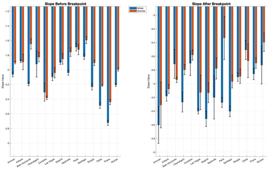
Figure 7.
Seasonal comparison of slopes before and after spectral breakpoint by city across diverse climatic and geographical contexts. Each bar represents the mean slope value for a given city, while error bars indicate the standard error of the mean (SEM) as a measure of uncertainty, reflecting variability within the dataset. The left panel focuses on slope values before the breakpoint, while the right panel illustrates slope values after the breakpoint.
3.6. Climatic Zone-Level Analysis Aggregated Patterns
The analysis of average spectral slopes for cities grouped by climatic zones (Figure 8) offers a nuanced understanding of deviations from the classical 2D turbulence hypothesis described by Kraichnan and Batchelor. By grouping cities into desert, humid continental, humid subtropical, Mediterranean, and oceanic climatic zones, the variations in spectral energy cascades before and after the breakpoint reveal how climatic factors modulate urban atmospheric turbulence.
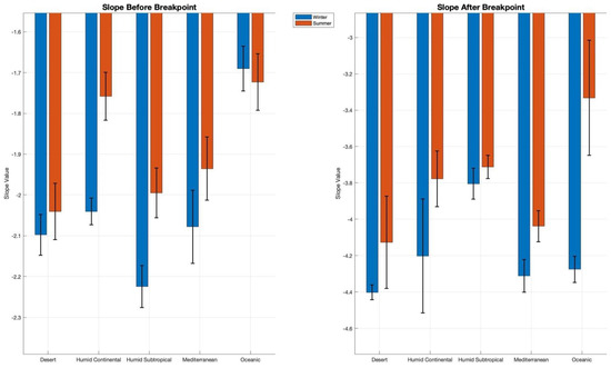
Figure 8.
Seasonal comparison of slopes before and after spectral breakpoint of the cities/locations under study grouped by climatic zone. Each bar represents the mean slope value for a given climatic zone, while error bars indicate the standard error of the mean (SEM) as a measure of uncertainty, reflecting variability within the dataset. The left panel depicts slope values before the breakpoint, while the right panel shows slope values after the breakpoint.
The slopes before the breakpoint highlight significant inter-climatic variation. The desert and humid subtropical zones exhibit steeper slopes (e.g., winter desert: K−2.09; humid subtropical: K−2.22), indicating less efficient energy transfer at larger scales, likely driven by limited vertical mixing due to thermal inversions in desert zones and enhanced heat and moisture fluxes in humid subtropical zones. Conversely, the oceanic zone shows the flattest slopes (winter: K−1.69; summer: K−1.72), reflecting relatively well-mixed conditions due to the moderating influence of maritime air masses. Seasonal variations are also evident. Winter generally features steeper slopes across all climatic zones, with values nearing the upper bound of the classical inverse energy cascade (K−3), reflecting the effects of increased stratification and reduced turbulence in colder months. Summer slopes are flatter, indicative of greater turbulence driven by solar heating and stronger vertical convection. Post-breakpoint slopes reveal significantly steeper dissipation patterns compared to the classical prediction of K−3, with notable differences between climatic zones. In winter, the desert and Mediterranean zones exhibit the steepest slopes (e.g., desert: K−4.49; Mediterranean: K−4.31), suggesting enhanced energy dissipation at smaller scales, possibly due to increased surface roughness and thermal stratification in these regions. Conversely, the humid subtropical zone has the flattest slopes (e.g., winter: K−3.80), reflecting weaker dissipation dynamics, possibly due to the higher moisture content and associated damping of small-scale turbulence. During summer, the oceanic zone consistently exhibits the flattest slopes (e.g., summer: K−3.33), indicating reduced dissipation compared to other climatic zones. This could be attributed to the oceanic climate’s characteristic smooth energy transfer facilitated by maritime influences and a lack of extreme thermal contrasts. Meanwhile, the desert zone (e.g., summer: K−4.21) maintains steep slopes, driven by persistent temperature extremes and limited vegetation cover, which enhance surface energy dissipation. The observed deviations from Kraichnan’s K−5/3 and K−3 scaling laws reveal distinct turbulence dynamics across climatic zones. Pre-breakpoint steeper slopes are observed in desert and humid subtropical zones, suggesting inefficient energy transfer at larger scales, linked to thermal stratification and urban heat flux variations. Flatter slopes in oceanic zones reflect well-mixed conditions facilitated by the moderating influence of maritime air, while post-breakpoint enhanced energy dissipation in desert and Mediterranean zones suggests strong thermal gradients and roughness effects. Reduced dissipation in humid subtropical and oceanic zones highlights the role of moisture and smoother surface conditions in moderating small-scale turbulence. These results underscore the influence of regional climatic conditions on urban turbulence. Desert zones are characterized by steeper slopes and enhanced dissipation across scales, reflecting the combined effects of extreme thermal contrasts and limited vegetation. Oceanic zones, in contrast, exhibit flatter slopes and smoother energy transfer due to the moderating influence of maritime air masses. The deviation from classical turbulence scaling laws across climatic zones highlights the need for localized parameterizations in urban thermal models. These findings can inform policies for urban planning and heat mitigation, particularly in desert and humid subtropical regions, where turbulence dynamics deviate significantly from classical predictions.
3.7. Linking Energy Processes to Spectral Characteristics
Our spectral analysis captures distinct energy transfer regimes, which correspond to the known SEB components and turbulence processes:
- Inverse energy cascade (large scales): At larger spatial scales (low wavenumbers), solar radiation, urban heat island (UHI) effects, and anthropogenic heat sources generate broad, persistent thermal structures. These large-scale anomalies retain energy due to the thermal inertia of urban materials, creating an inverse cascade, where energy accumulates rather than dissipates immediately. The spectral slopes before the breakpoint (~K−1.6 to ~K−2.7 in winter and ~K−1.5 to ~K−2.4 in summer) indicate sustained energy at these larger scales.
- Spectral breakpoint and transition to direct cascade: The breakpoint represents the scale at which energy transitions from retention to dissipation, marking the point where convective turbulence begins to break down large-scale thermal structures. This shift corresponds to the onset of vertical mixing, where sensible heat flux (H) plays a dominant role in transferring heat into the urban boundary layer.
- Direct energy cascade (small scales): At smaller spatial scales (high wavenumbers), energy is transferred into fine-scale turbulent eddies, where it is dissipated through radiative cooling, conduction, and small-scale convective mixing. The steeper spectral slopes post-breakpoint (~K−3.5 to ~K−4.6 in winter and ~K−3.3 to ~K−4.3 in summer) indicate an increased rate of energy loss, confirming that heat dissipation dominates at these finer spatial scales.
- Seasonal and climatic modulation of energy transfer: The spectral differences between summer and winter align with the expected seasonal variations in SEB components. In summer, higher solar radiation and stronger convective mixing lead to more gradual energy dissipation, sustaining larger-scale temperature structures. In winter, weaker solar forcing and stable atmospheric conditions suppress vertical mixing, increasing energy loss at small scales. Similarly, climatic zone differences (e.g., steeper post-breakpoint slopes in desert and Mediterranean cities) reflect how regional climate influences heat dissipation efficiency.
4. Conclusions
This study provides a novel spectral analysis of urban heat island (UHI) dynamics across 14 cities in different climatic zones, revealing systematic deviations from the classical two-dimensional (2D) turbulence hypothesis. By examining the spatial power spectra of land surface temperature (LST) variations over multiple decades, we quantified how energy cascades and spectral breakpoints diverge from theoretical predictions, offering new insights into urban thermal turbulence across scales.
Our findings indicate that spectral breakpoints serve as a robust metric for identifying the transition between large-scale energy retention processes and small-scale dissipative mechanisms. The variability in spectral slopes across different cities highlights the significant role of urban morphology, climate, and seasonal factors in shaping urban energy distributions. Cities with denser urban cores and greater surface heterogeneity exhibited steeper spectral slopes, indicative of enhanced small-scale energy dissipation, whereas more spatially homogeneous cities demonstrated smoother transitions across scales. A key discovery is the systematic deviation from classical turbulence scaling laws. Before the spectral breakpoint, slopes ranged from ~K−1.6 to ~K−2.7 during winter and ~K−1.5 to ~K−2.4 during summer, while after the breakpoint, the slopes steepened significantly to ~K−3.5 to ~K−4.6 in winter and ~K−3.3 to ~K−4.3 in summer. These deviations suggest that urban heat turbulence is governed by a combination of buoyancy-driven convection, wake turbulence, and mesoscale instabilities, deviating from the expected K−5/3 and K−3 spectral scaling predicted by classical 2D turbulence. Seasonal variations further modulate these spectral deviations, with summer conditions characterized by enhanced vertical mixing, stronger convective processes, and chaotic turbulence at smaller scales. In contrast, winter conditions led to stabilized boundary layers, smoother spectral transitions, and a dominance of horizontal energy transport over vertical convection. These results emphasize that urban energy dynamics cannot be generalized across seasons and require a scale-dependent approach to accurately capture the complexity of urban heat transfer processes. At the climatic zone level, we observed distinct turbulence regimes. Desert and Mediterranean cities exhibited the steepest spectral slopes post-breakpoint, reflecting enhanced small-scale energy dissipation due to extreme thermal gradients and surface roughness effects. Conversely, oceanic and humid subtropical cities displayed flatter slopes, indicative of more efficient energy transfer and reduced dissipation, likely due to the moderating effects of maritime influences and moisture availability. These results demonstrate that urban thermal turbulence is not only modulated by local urban structures but also by broader regional climatic factors, reinforcing the need for climate-specific urban climate models.
The implications of these findings extend to urban planning, climate resilience, and energy-efficient city design. Understanding how turbulence-driven energy dissipation varies across scales can inform targeted UHI mitigation strategies, such as optimizing green infrastructure placement, enhancing urban ventilation corridors, and adjusting building materials to minimize heat retention at critical scales. By integrating spectral analysis with urban climate modeling, future research can refine the parameterizations of urban energy fluxes, improving the predictions of urban climate dynamics under future warming scenarios.
This study provides a foundational framework for incorporating turbulence theory into urban heat island research, bridging the gap between theoretical fluid dynamics and empirical urban climate analysis. The consistent deviations from classical turbulence laws observed across all cities underscore the uniqueness of urban thermal turbulence, necessitating new approaches to account for anisotropy, mesoscale structures, and heterogeneous surface energy exchanges in urban boundary layers. Future research should expand this methodology to additional cities, incorporate finer-scale observational datasets, and further explore the role of anthropogenic heat sources in modulating spectral energy distributions. By advancing our understanding of the spectral characteristics of urban heat turbulence, this work contributes to the broader discourse on sustainable urban development in a rapidly warming world.
Author Contributions
Conceptualization, methodology, and formal analysis, G.I.C., J.C.J. and J.A.S.; software, resources, and data curation, G.I.C.; writing—original draft preparation, G.I.C.; writing—review and editing, G.I.C., J.C.J. and J.A.S. All authors have read and agreed to the published version of the manuscript.
Funding
This research received no external funding.
Data Availability Statement
Data used in this research are available upon reasonable request from the authors.
Conflicts of Interest
The authors declare no conflicts of interest.
References
- Grimmond, S. Urbanization and global environmental change: Local effects of urban warming. Geogr. J. 2007, 173, 83–88. [Google Scholar] [CrossRef]
- McManamay, R.A.; Vernon, C.R.; Chen, M.; Thompson, I.; Khan, Z.; Narayan, K.B. Dynamic urban land extensification is projected to lead to imbalances in the global land-carbon equilibrium. Commun. Earth Environ. 2024, 5, 70. [Google Scholar] [CrossRef]
- Gao, J.; O’Neill, B.C. Mapping global urban land for the 21st century with data-driven simulations and Shared Socioeconomic Pathways. Nat. Commun. 2020, 11, 2302. [Google Scholar] [CrossRef]
- Zhou, D.; Xiao, J.; Bonafoni, S.; Berger, C.; Deilami, K.; Zhou, Y.; Frolking, S.; Yao, R.; Qiao, Z.; Sobrino, J.A. Satellite Remote Sensing of Surface Urban Heat Islands: Progress, Challenges, and Perspectives. Remote Sens. 2018, 11, 48. [Google Scholar] [CrossRef]
- Huang, F.; Zhan, W.; Wang, Z.-H.; Voogt, J.; Hu, L.; Quan, J.; Liu, C.; Zhang, N.; Lai, J. Satellite identification of atmospheric-surface-subsurface urban heat islands under clear sky. Remote Sens. Environ. 2020, 250, 112039. [Google Scholar] [CrossRef]
- Weng, Q.; Larson, R.C. Satellite Remote Sensing of Urban Heat Islands: Current Practice and Prospects. In Geo-Spatial Technologies in Urban Environments; Springer: Berlin/Heidelberg, Germany, 2005. [Google Scholar] [CrossRef]
- Hurduc, A.; Ermida, S.L.; DaCamara, C.C. On the Suitability of Different Satellite Land Surface Temperature Products to Study Surface Urban Heat Islands. Remote Sens. 2024, 16, 3765. [Google Scholar] [CrossRef]
- Zhang, W.; Li, Y.; Zheng, C.; Zhu, Y. Surface urban heat island effect and its driving factors for all the cities in China: Based on a new batch processing method. Ecol. Indic. 2023, 146, 109818. [Google Scholar] [CrossRef]
- Kabisch, N.; Remahne, F.; Ilsemann, C.; Fricke, L. The urban heat island under extreme heat conditions: A case study of Hannover, Germany. Sci. Rep. 2023, 13, 23017. [Google Scholar] [CrossRef]
- Garuma, G.F. Tropical surface urban heat islands in east Africa. Sci. Rep. 2023, 13, 4509. [Google Scholar] [CrossRef]
- Oke, T.R. The energetic basis of the urban heat island. Q. J. R. Meteorol. Soc. 1982, 108, 1–24. [Google Scholar] [CrossRef]
- Oke, T.R. The Heat Island of the Urban Boundary Layer: Characteristics, Causes and Effects. Wind. Clim. Cities 1995, 277, 81–107. [Google Scholar] [CrossRef]
- Xian, J.; Qiu, Z.; Luo, H.; Hu, Y.; Lin, X.; Lu, C.; Yang, Y.; Yang, H.; Zhang, N. Turbulent energy budget analysis based on coherent wind lidar observations. Atmos. Chem. Phys. 2025, 25, 441–457. [Google Scholar] [CrossRef]
- Aliabadi, A.A.; Moradi, M.; Byerlay, R.A.E. The budgets of turbulence kinetic energy and heat in the urban roughness sublayer. Environ. Fluid Mech. 2021, 21, 843–884. [Google Scholar] [CrossRef]
- Kalogeropoulos, G.; Dimoudi, A.; Toumboulidis, P.; Zoras, S. Urban Heat Island and Thermal Comfort Assessment in a Medium-Sized Mediterranean City. Atmosphere 2022, 13, 1102. [Google Scholar] [CrossRef]
- Sarker, T.; Fan, P.; Messina, J.P.; Macatangay, R.; Varnakovida, P.; Chen, J. Land surface temperature and trans-boundary air pollution: A case of Bangkok Metropolitan Region. Sci. Rep. 2024, 14, 10955. [Google Scholar] [CrossRef] [PubMed]
- Hsu, A.; Sheriff, G.; Chakraborty, T.; Manya, D. Disproportionate exposure to urban heat island intensity across major US cities. Nat. Commun. 2021, 12, 2721. [Google Scholar] [CrossRef]
- Santamouris, M.; Cartalis, C.; Synnefa, A.; Kolokotsa, D. On the impact of urban heat island and global warming on the power demand and electricity consumption of buildings—A review. Energy Build. 2015, 98, 119–124. [Google Scholar] [CrossRef]
- Hidalgo-García, D.; Arco-Díaz, J. Spatiotemporal analysis of the surface urban heat island (SUHI), air pollution and disease pattern: An applied study on the city of Granada (Spain). Environ. Sci. Pollut. Res. 2023, 30, 57617–57637. [Google Scholar] [CrossRef]
- Barlow, J.F. Progress in observing and modelling the urban boundary layer. Urban Clim. 2014, 10, 216–240. [Google Scholar] [CrossRef]
- Arnfield, A.J. Two decades of urban climate research: A review of turbulence, exchanges of energy and water, and the urban heat island. Int. J. Climatol. 2003, 23, 1–26. [Google Scholar] [CrossRef]
- Kolmogorov, A.N. Dissipation of Energy in the Locally Isotropic Turbulence Mathematical and Physical Sciences Vol. 434, No. 1890, Turbulence and Stochastic Process: Kolmogorov’s Ideas 50 Years on (Jul. 8, 1991), pp. 15–17 (3 Pages) Royal Society. Available online: https://www.jstor.org/stable/i203079 (accessed on 20 January 2025).
- Batchelor, G.K. Small-scale variation of convected quantities like temperature in turbulent fluid Part 1. General discussion and the case of small conductivity. J. Fluid Mech. 1959, 5, 113. [Google Scholar] [CrossRef]
- Kraichnan, R.H. Inertial Ranges in Two-Dimensional Turbulence. Phys. Fluids 1967, 10, 1417–1423. [Google Scholar] [CrossRef]
- Liu, H.; Yuan, R.; Mei, J.; Sun, J.; Liu, Q.; Wang, Y. Scale Properties of Anisotropic and Isotropic Turbulence in the Urban Surface Layer. Bound.-Layer Meteorol. 2017, 165, 277–294. [Google Scholar] [CrossRef]
- Roth, M.; Oke, T. Turbulent transfer relationships over an urban surface. I: Spectral characteristics. Q. J. R. Meteorol. Soc. 1993, 119, 1071–1104. [Google Scholar] [CrossRef]
- Horiguchi, M.; Tatsumi, K.; Poulidis, A.-P.; Yoshida, T.; Takemi, T. Large-Scale Turbulence Structures in the Atmospheric Boundary Layer Observed above the Suburbs of Kyoto City, Japan. Bound.-Layer Meteorol. 2022, 184, 333–354. [Google Scholar] [CrossRef]
- Fortuniak, K.; Pawlak, W. Selected Spectral Characteristics of Turbulence over an Urbanized Area in the Centre of Łódź, Poland. Bound.-Layer Meteorol. 2014, 154, 137–156. [Google Scholar] [CrossRef]
- Nordbo, A.; Järvi, L.; Haapanala, S.; Moilanen, J.; Vesala, T. Intra-City Variation in Urban Morphology and Turbulence Structure in Helsinki, Finland. Bound.-Layer Meteorol. 2012, 146, 469–496. [Google Scholar] [CrossRef]
- Roth, M.; Salmond, J.A.; Satyanarayana, A.N.V. Methodological Considerations Regarding the Measurement of Turbulent Fluxes in the Urban Roughness Sublayer: The Role of Scintillometery. Bound.-Layer Meteorol. 2006, 121, 351–375. [Google Scholar] [CrossRef]
- Fernando, H.J.S. Fluid mechanics of urban atmospheres in complex terrain. Annu. Rev. Fluid Mech. 2010, 42, 365–389. [Google Scholar] [CrossRef]
- Roth, M. Review of atmospheric turbulence over cities. Q. J. R. Meteorol. Soc. 2000, 126, 941–990. [Google Scholar] [CrossRef]
- Garai, A.; Pardyjak, E.; Steeneveld, G.-J.; Kleissl, J. Surface Temperature and Surface-Layer Turbulence in a Convective Boundary Layer. Bound.-Layer Meteorol. 2013, 148, 51–72. [Google Scholar] [CrossRef]
- Bou-Zeid, E.; Meneveau, C.; Parlange, M.B. Large-eddy simulation of neutral atmospheric boundary layer flow over heterogeneous surfaces: Blending height and effective surface roughness. Water Resour. Res. 2004, 40. [Google Scholar] [CrossRef]
- Tian, G.; Conan, B.; Calmet, I. Turbulence-Kinetic-Energy Budget in the Urban-Like Boundary Layer Using Large-Eddy Simulation. Bound.-Layer Meteorol. 2020, 178, 201–223. [Google Scholar] [CrossRef]
- Kanda, M. Large-Eddy Simulations on the Effects of Surface Geometry of Building Arrays on Turbulent Organized Structures. Bound.-Layer Meteorol. 2006, 118, 151–168. [Google Scholar] [CrossRef]
- Li, W.; Giometto, M.G. The structure of turbulence in unsteady flow over urban canopies. J. Fluid Mech. 2024, 985, A5. [Google Scholar] [CrossRef]
- Margairaz, F.; Pardyjak, E.R.; Calaf, M. Surface Thermal Heterogeneities and the Atmospheric Boundary Layer: The Relevance of Dispersive Fluxes. Bound.-Layer Meteorol. 2020, 175, 369–395. [Google Scholar] [CrossRef]
- Wang, W. The Influence of Thermally-Induced Mesoscale Circulations on Turbulence Statistics Over an Idealized Urban Area Under a Zero Background Wind. Bound.-Layer Meteorol. 2009, 131, 403–423. [Google Scholar] [CrossRef]
- Sha, J.; Zou, J.; Sun, J. Observational study of land-atmosphere turbulent flux exchange over complex underlying surfaces in urban and suburban areas. Sci. China Earth Sci. 2021, 64, 1050–1064. [Google Scholar] [CrossRef]
- Grimmond, C.S.B.; Salmond, J.A.; Oke, T.R.; Offerle, B.; Lemonsu, A. Flux and turbulence measurements at a densely built-up site in Marseille: Heat, mass (water and carbon dioxide), and momentum. J. Geophys. Res. Atmos. 2004, 109. [Google Scholar] [CrossRef]
- Offerle, B.; Grimmond, C.S.B.; Fortuniak, K. Heat storage and anthropogenic heat flux in relation to the energy balance of a central European city center. Int. J. Climatol. 2005, 25, 1405–1419. [Google Scholar] [CrossRef]
- Piringer, M.; Grimmond, C.S.B.; Joffre, S.M.; Mestayer, P.; Middleton, D.R.; Rotach, M.W.; Baklanov, A.; De Ridder, K.; Fer-reira, J.; Guilloteau, E.; et al. Investigating the Surface Energy Balance in Urban Areas—Recent Advances and Future Needs. Urban Air Qual.—Recent Adv. 2002, 1–16. [Google Scholar] [CrossRef]
- Guo, F.; Sun, J.; Hu, D. Surface energy balance-based surface urban heat island decomposition at high resolution. Remote Sens. Environ. 2024, 315, 114447. [Google Scholar] [CrossRef]
- Feigenwinter, C.; Vogt, R. Detection and analysis of coherent structures in urban turbulence. Theor. Appl. Climatol. 2005, 81, 219–230. [Google Scholar] [CrossRef]
- Christen, A.; van Gorsel, E.; Vogt, R. Coherent structures in urban roughness sublayer turbulence. Int. J. Climatol. 2007, 27, 1955–1968. [Google Scholar] [CrossRef]
- Inagaki, A.; Kanda, M.; Ahmad, N.H.; Yagi, A.; Onodera, N.; Aoki, T. A Numerical Study of Turbulence Statistics and the Structure of a Spatially-Developing Boundary Layer Over a Realistic Urban Geometry. Bound.-Layer Meteorol. 2017, 164, 161–181. [Google Scholar] [CrossRef]
- de Wit, X.M.; Fruchart, M.; Khain, T.; Toschi, F.; Vitelli, V. Pattern formation by turbulent cascades. Nature 2024, 627, 515–521. [Google Scholar] [CrossRef]
- Zajic, D.; Fernando, H.J.S.; Calhoun, R.; Princevac, M.; Brown, M.J.; Pardyjak, E.R. Flow and Turbulence in an Urban Canyon. J. Appl. Meteorol. Climatol. 2011, 50, 203–223. [Google Scholar] [CrossRef]
- Mazzeo, N.A.; Venegas, L.E. Study of natural and traffic-producing turbulences analysing full-scale data from four street canyons. Int. J. Environ. Pollut. 2011, 47, 290. [Google Scholar] [CrossRef]
- Liu, P.; Liu, C.; Li, Q. Effects of landscape pattern on land surface temperature in Nanchang, China. Sci. Rep. 2024, 14, 3832. [Google Scholar] [CrossRef]
- Ayanlade, A.; Aigbiremolen, M.I.; Oladosu, O.R. Variations in urban land surface temperature intensity over four cities in different ecological zones. Sci. Rep. 2021, 11, 20537. [Google Scholar] [CrossRef]
- Akomolafe, G.F.; Rosazlina, R. Land use and land cover changes influence the land surface temperature and vegetation in Penang Island, Peninsular Malaysia. Sci. Rep. 2022, 12, 21250. [Google Scholar] [CrossRef] [PubMed]
- Boffetta, G.; Ecke, R.E. Two-Dimensional Turbulence. Annu. Rev. Fluid Mech. 2012, 44, 427–451. [Google Scholar] [CrossRef]
- Oke, T.R. Boundary Layer Climates; Routledge: London, UK, 1987. [Google Scholar]
- Voogt, J.A.; Oke, T.R. Thermal remote sensing of urban climates. Remote Sens. Environ. 2003, 86, 370–384. [Google Scholar] [CrossRef]
- Li, Y.; Schubert, S.; Kropp, J.P.; Rybski, D. On the influence of density and morphology on the Urban Heat Island intensity. Nat. Commun. 2020, 11, 2647. [Google Scholar] [CrossRef]
- Chapman, S.; Thatcher, M.; Salazar, A.; Watson, J.E.M.; McAlpine, C.A. The Effect of Urban Density and Vegetation Cover on the Heat Island of a Subtropical City. J. Appl. Meteorol. Climatol. 2018, 57, 2531–2550. [Google Scholar] [CrossRef]
- Grimmond, C.S.B.; Oke, T.R. Heat Storage in Urban Areas: Local-Scale Observations and Evaluation of a Simple Model. J. Appl. Meteorol. 1999, 38, 922–940. [Google Scholar] [CrossRef]
- Incropera, F.P.; DeWitt, D.P. Introduction to Heat Transfer; John Wiley and Sons: New York, NY, USA, 1990. [Google Scholar]
- Grimmond, C.S.B.; Oke, T.R. Turbulent Heat Fluxes in Urban Areas: Observations and a Local-Scale Urban Meteorological Parameterization Scheme (LUMPS). J. Appl. Meteorol. 2002, 41, 792–810. [Google Scholar] [CrossRef]
- Beck, H.; Zimmermann, N.; McVicar, T.; Vergopolan, N.; Berg, A.; Wood, E.F. Present and future Köppen-Geiger climate classification maps at 1-km resolution. Sci. Data 2018, 5, 180214. [Google Scholar] [CrossRef]
- Available online: https://daylightmap.org/2023/11/27/urban.html (accessed on 15 December 2024).
- QGIS Development Team. QGIS Version 3.34. Geographic Information System. Open-Source Geospatial Foundation Project. 2024. Available online: https://www.qgis.org/en/site/ (accessed on 10 August 2024).
- MathWorks 2024. MATLAB Ver. 2024a Computer Program. (The MathWorks Inc., 2024). Available online: https://www.mathworks.com/ (accessed on 11 November 2024).
- Available online: http://turbustat.readthedocs.org/en/latest/ (accessed on 10 November 2024).
- Python Software Foundation. Python Language Reference, Version 3.11.5. Available online: https://www.python.org (accessed on 10 August 2024).
- Bou-Zeid, E.; Anderson, W.; Katul, G.G.; Mahrt, L. The Persistent Challenge of Surface Heterogeneity in Boundary-Layer Meteorology: A Review. Bound.-Layer Meteorol. 2020, 177, 227–245. [Google Scholar] [CrossRef]
- Ward, H.C.; Rotach, M.W.; Gohm, A.; Graus, M.; Karl, T.; Haid, M.; Umek, L.; Muschinski, T. Energy and mass exchange at an urban site in mountainous terrain—The Alpine city of Innsbruck. Atmos. Chem. Phys. 2022, 22, 6559–6593. [Google Scholar] [CrossRef]
- Rios, G.; Ramamurthy, P. Turbulence in the Mixed Layer Over an Urban Area: A New York City Case Study. Bound.-Layer Meteorol. 2023, 188, 419–440. [Google Scholar] [CrossRef]
- Alcayaga, L.; Larsen, G.C.; Kelly, M.; Mann, J. Large-Scale Coherent Turbulence Structures in the Atmospheric Boundary Layer over Flat Terrain. J. Atmos. Sci. 2022, 79, 3219–3243. [Google Scholar] [CrossRef]
- Chen, Y.; Yang, J.; Yu, W.; Ren, J.; Xiao, X.; Xia, J.C. Relationship between urban spatial form and seasonal land surface temperature under different grid scales. Sustain. Cities Soc. 2023, 89, 104374. [Google Scholar] [CrossRef]
- Schwaab, J.; Meier, R.; Mussetti, G.; Seneviratne, S.; Bürgi, C.; Davin, E.L. The role of urban trees in reducing land surface temperatures in European cities. Nat. Commun. 2021, 12, 6763. [Google Scholar] [CrossRef] [PubMed]
Disclaimer/Publisher’s Note: The statements, opinions and data contained in all publications are solely those of the individual author(s) and contributor(s) and not of MDPI and/or the editor(s). MDPI and/or the editor(s) disclaim responsibility for any injury to people or property resulting from any ideas, methods, instructions or products referred to in the content. |
© 2025 by the authors. Licensee MDPI, Basel, Switzerland. This article is an open access article distributed under the terms and conditions of the Creative Commons Attribution (CC BY) license (https://creativecommons.org/licenses/by/4.0/).