Study on Ecosystem Service Values of Urban Green Space Systems in Suzhou City Based on the Extreme Gradient Boosting Geographically Weighted Regression Method: Spatiotemporal Changes, Driving Factors, and Influencing Mechanisms

Abstract

Urban green space systems (UGSS) play a crucial role in enhancing citizens’ well-being and promoting sustainable urban development through their ecosystem service values (ESV). However, understanding the spatiotemporal changes, driving factors, and influencing mechanisms of ESV remains a critical challenge for advancing urban green theories and formulating effective policies. This study focuses on Suzhou, China’s third-largest prefecture-level city by economic volume and ecological core city of the Taihu watershed, to evaluate the ESV of its UGSS from 2010 to 2020, identify key driving factors, and analyze their influencing mechanisms. Using the InVEST model combined with the entropy weight method (EWM), we assessed the ESV changes over the study period. To examine the influencing mechanisms, we employed an innovative XGBoost-GWR approach, where XGBoost was used to screen globally significant factors from 37 potential drivers, and geographically weighted regression (GWR) was applied to model local spatial heterogeneity, providing a research perspective that balances global nonlinear relationships with local spatial heterogeneity. The results revealed three key findings: First, while Suzhou’s UGSS ESV increased by 9.92% from 2010 to 2020, the Global Moran’s I index rose from 0.325 to 0.489, indicating that its spatial distribution became more uneven, highlighting the increased ecological risks. Second, climate, topography, landscape pattern, and vegetation emerged as the most significant driving factors, with topographic factors showing the greatest variation (the negatively impacted area increased by 455.60 km²) and climate having the largest overall impact but least variation. Third, the influencing mechanisms were primarily driven by land use changes resulting from urbanization and industrialization, leading to increased ecological risks such as soil erosion, pollution, landscape fragmentation, and habitat degradation, particularly in the Kunshan, Wujiang, and Zhangjiagang Districts, where agricultural land has been extensively converted to constructed land. This study not only elucidates the mechanisms influencing UGSS’s ESV driving factors but also expands the theoretical understanding of urbanization’s ecological impacts, providing valuable insights for optimizing UGSS layout and informing sustainable urban planning policies.

1. Introduction

Ecosystem service value (ESV) refers to the benefits that ecosystems provide to human society through their structure, processes, and functions, such as carbon storage, soil conservation, pollutant absorption etc., all of which enhance human well-being, economic resilience, and long-term ecological security. The urban green space system (UGSS), which includes urban green spaces (UGS), agricultural land, and green belts, forms an integrated ecological network and serves as the primary provider of ESV [1,2]. UGSS plays a vital role in modern urban development by delivering essential services such as carbon sequestration, habitat provision, and pollutant absorption [3,4], which are crucial for enhancing citizens’ well-being, ensuring ecological security, and supporting regional sustainable development [5]. Understanding the ESV of UGSS and its influencing mechanisms is therefore critical for mitigating the adverse effects of urban expansion and industrialization, as well as for informing policies to optimize UGSS layout and alleviate ecological pressures.

The concept of ESV was first introduced by Costanza in his research on natural capital [6,7]. Current studies focus on three main areas: spatiotemporal dynamics [8], trade-off/synergy relationships [9], and driving mechanisms [10]. Core assessment targets include carbon sequestration, water yield, soil conservation, and habitat quality. Researchers employ multi-model approaches, such as the equivalent factor method, InVEST, CASA, and RUSLE, to quantify ecosystem services. These are complemented by spatial analysis techniques like geographical detectors, geographically weighted regression (GWR), and principal component analysis (PCA) to identify socio-natural drivers, including urbanization [11], climate [12], and policy [13]. However, selecting appropriate driving factors remains challenging due to the unique geographical and developmental characteristics of different cities [14]. Traditional methods, which rely on ecological theory, literature reviews, and domain knowledge [15], may introduce human bias and limit predictive accuracy. Additionally, existing regression models, such as global regression and spatial regression, have limitations: global regression cannot explain regional variations, while spatial regression lacks mechanisms for automatic factor selection.

To address these limitations, this study combines the XGBoost algorithm with geographically weighted regression (GWR). Compared to traditional approaches that separately handle global features and local heterogeneity, the XGBoost-GWR integrated framework dynamically couples both. XGBoost captures global nonlinear relationships through ensemble learning and selects key driving factors, while GWR dissects spatial heterogeneity using spatial weight matrices. This integration overcomes the limitations of traditional models, such as ordinary linear regression or individual machine learning models, in addressing spatial hierarchical nesting and provides a research perspective that balances global nonlinear relationships with local spatial heterogeneity [16]. In addition, compared to other machine learning approaches combined with spatial regression, XGBoost’s regularization and pruning techniques prevent overfitting and ensure stable feature importance scores, outperforming alternatives like random forest and neural networks. This dual optimization enhances both the interpretability and accuracy of the analysis.

This study focuses on Suzhou, a megacity in the Taihu watershed and a representative case of urbanization and industrialization. Suzhou ranks third among China’s prefecture-level cities in economic volume, with its growth heavily reliant on urban and industrial development [17]. According to the local statistical yearbook, the urbanization rate of Suzhou increased from 70.6% in 2010 to 81.7% in 2020, while the Gross Industrial Output Value of Enterprises Above Designated Size increased from CNY 24,651.67 billion to CNY 35,342.55 billion, highlighting the rapid industrialization and urbanization (Figure 1). In addition, Suzhou is the ecological core city in the Taihu Lake watershed, adjacent to Taihu Lake, the third-largest freshwater resource in China. The quality of its ecological environment will play an important ecological role in the Taihu Lake watershed. Decades of rapid urbanization have led to severe ecological challenges, including pollution, soil erosion, and water quality deterioration in Taihu Lake [18]. Despite local government efforts, these issues persist, threatening both local and regional ecological security [19,20,21]. Despite these challenges, there is limited research on the comprehensive evaluation of UGSS’s ESV and its influencing mechanisms in Suzhou. This study aims to address Suzhou’s ecological challenges by offering a comprehensive evaluation of the ESV of its UGSS and identifying key influencing factors. It will analyze the impact of Suzhou’s rapid urbanization and industrialization on the urban green space system, evaluate the weakening or change in ESV in industrial and urban expansion areas, examine the spatial differences of the mechanisms of impact factors in different regions, and analyze the potential ecological risks in the study area. Its detailed objectives, conclusions, and functions include the following:

(1) Analyzing the spatiotemporal changes in ESV of UGSS in Suzhou and identifying the ecological challenges posed by rapid urbanization highlights the ecological risks associated with uneven distribution. This finding deepens the understanding of the overall spatiotemporal evolution of ESV under rapid urbanization and provides a foundation for targeted interventions to address regional disparities.

(2) Identifying the key driving factors of ESV and examining their influencing mechanisms across different regions of Suzhou reveal that climate, topography, landscape pattern, and vegetation are key drivers of ESV, with urbanization and industrialization shaping their impacts, thereby offering insights into region-specific ecological challenges. This understanding is helpful for proposing targeted measures to improve ESV according to the actual conditions in different regions.

(3) Providing targeted recommendations for optimizing UGSS layout to enhance sustainable development and ecological security is essential. The findings support urban planners in crafting policies to optimize UGSS layout, mitigate ecological risks, and promote sustainable development. The integration of XGBoost and GWR provides a robust framework for analyzing ESV, advancing both theoretical understanding and practical applications in urban green space management.

2. Research Materials and Study Methods

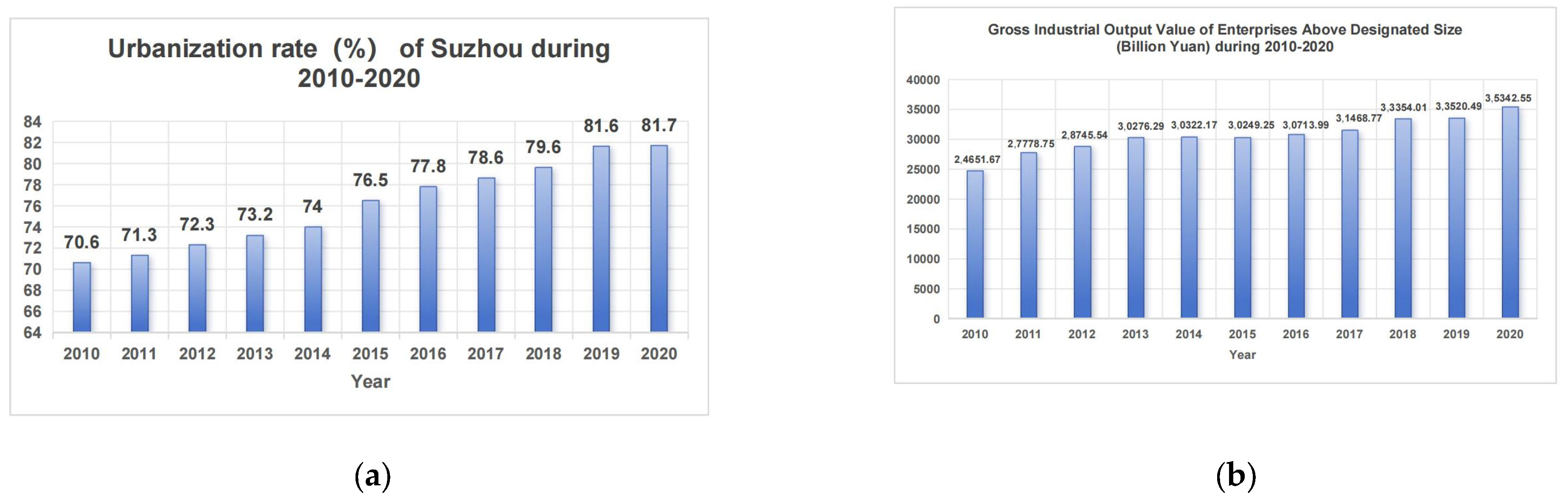
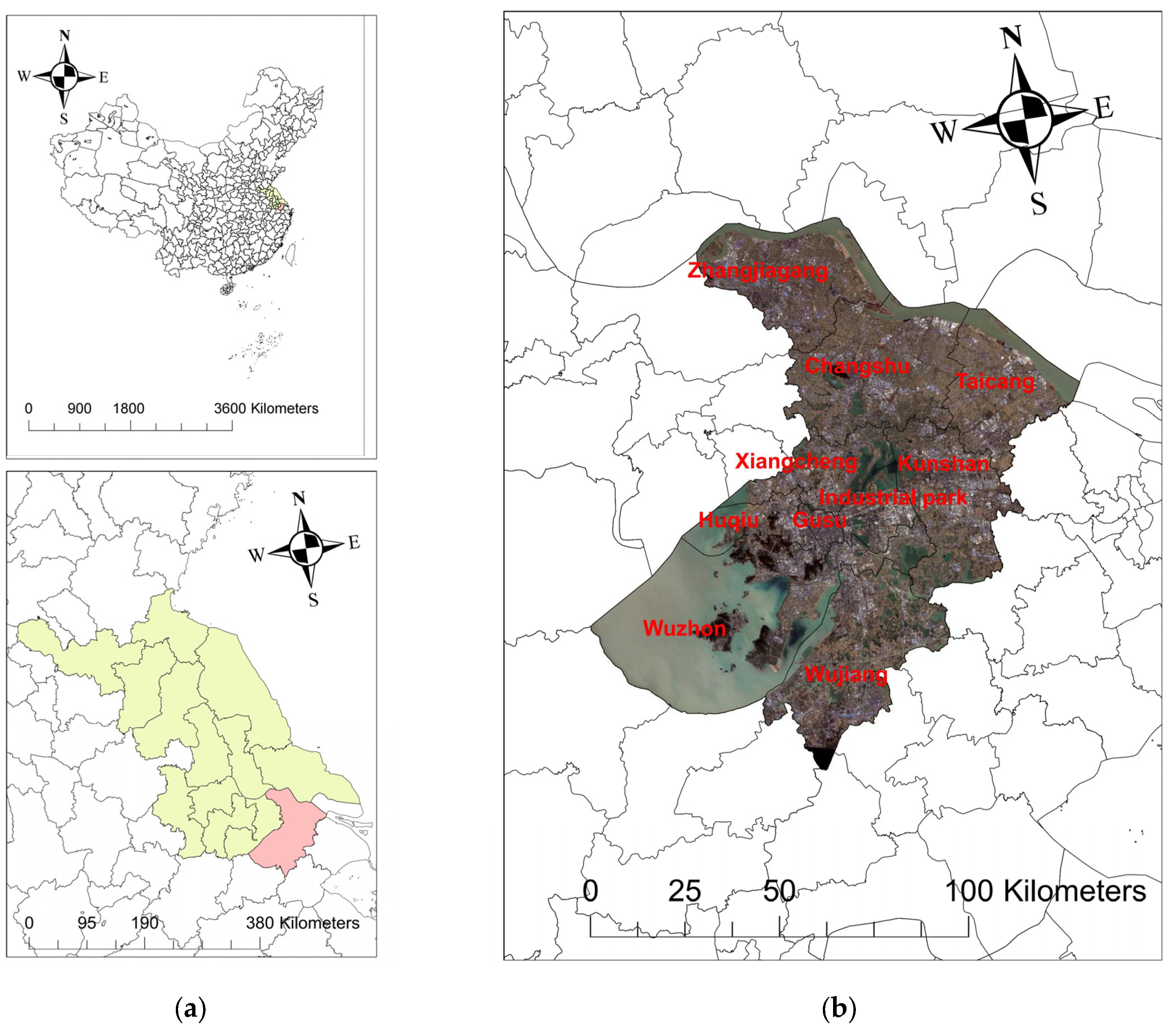
2.1. Study Area

Suzhou City is located in the eastern part of Jiangsu Province, China, in the core area of the Yangtze River Delta and Taihu Lake Basin. Its geographical coordinates range from 30°46′ to 32°02′ north latitude and from 120°11′ to 121°16′ east longitude. The city lies within a subtropical monsoon climate zone, characterized by four distinct seasons and a mild climate with moderate temperatures. The annual average temperature is approximately 15.7 °C, and the annual average precipitation is 1100 mm. As the core area of the Taihu Lake Basin, Suzhou’s ecological importance cannot be ignored. Taihu Lake, the third-largest freshwater lake in China, plays a crucial role in maintaining the ecological balance and managing water resources for the surrounding areas. The ecological security of Suzhou is not only vital to local economic development and environmental protection but also holds significant importance for the overall health of the Taihu Lake Basin (Figure 2).

By researching and identifying the key factors and influencing mechanisms affecting the ecosystem services of Suzhou City’s UGSS, scientific planning and management guidelines can be provided for cities in important ecological watersheds. This ensures that their green space systems can continuously provide essential ecosystem services and safeguard regional ecological security.

Suzhou governs six districts (Gusu, Wuzhong, Xiangcheng, Huqiu, Wujiang, and the Industrial Park) and four county-level cities (Changshu, Zhangjiagang, Kunshan, and Taicang). By 2020, Suzhou had a permanent resident population of 10.75 million and a regional GDP of USD 2765.193 billion. As an important city in Jiangsu Province, Suzhou has undergone significant changes in its urbanization process and industrial development. Since the 1990s, it has entered a stage of accelerated development. By 2015, Suzhou’s urbanization level had reached a stage of steady development, with an average annual growth rate of 4.79%. In terms of industry, since the Reform and Opening-up, Suzhou has relied on the rapid development of township enterprises, leading to significant economic growth. However, as urbanization and industrialization have progressed, ecological problems such as pollution and habitat degradation have gradually emerged. The Suzhou municipal government and relevant departments are actively implementing measures to ensure the continued provision of ecological services, including ecological restoration and the construction of green corridors. Despite these efforts, Suzhou continues to face significant ecological challenges, including water pollution and soil erosion.

2.2. Data Sources

The data used in this paper include land use and land cover (LULC) maps, various influencing factors, and inVEST model calculation data. The natural influencing factors and remote sensing data come from the Google Earth Engine (GEE) platform [22,23]. LULC maps were computed using the random forest (RF) algorithm based on Landsat-7 SR remote sensing images from the Landsat 7 Surface Reflectance dataset, a project of the United States Geological Survey (USGS). The main socioeconomic data come from the National Science Data Center for Resources and Environmental Sciences, Chinese Academy of Sciences. The inVEST models used in this study include (1) the sediment delivery ratio; (2) annual water yield; (3) habitat quality; (4) carbon storage; and (5) the nutrient delivery rate. These five indicators can represent the main ESV of UGSS, which can concentrate on reflecting the regional services of UGSS. ESVs like crop production, urban cooling, urban stormwater management, etc., mainly reflect the value of particular types of green space (like agricultural areas, urban parks, etc.) and cannot reflect the overall value of the urban green space system. The selection of factors needs to comprehensively and systematically reflect the main drivers that are dynamic and external and affect the urban green space ecosystem, covering multiple aspects such as the natural environment, socioeconomic factors, etc. This article refers to previous research and collects relevant influencing factors as comprehensively as possible for screening. The data on driving factors include (1) Climate factors: precipitation, evaporation, wind speed, surface temperature, sunshine duration, soil moisture, soil temperature, and runoff; (2) Topographical factors: elevation and slope; (3) Vegetation factors: leaf area index (LAI), Normalized Difference Vegetation Index (NDVI), and net primary productivity (NPP); (4) Socioeconomic factors: population density, GDP distribution, and night light intensity; and (5) Landscape pattern factors, computed using Fragstats 4.2 software and LULC maps. The calculation method is the 500 m × 500 m moving window method. In addition, the 19 indices we chose include Ai, Cohesion, Contag, Division, Iji, Lpi, Lsi, Mesh, Msidi, Meiei, Np, Pafrac, Pd, Pladj, Shdi, Shei, Sidi, Siei, and split. See

Table 1. Data and sources used in this study.

Data Name	Source
Remote Sensing Imagery Data	Landsat 7 Surface Reflectance dataset, United States Geological Survey(USGS).
Land Use and Land Cover Change Data (LULC)	computed based on remote sensing imagery data by random forest algorithm based on remote sensing imagery data from Landsat 7 Surface Reflectance dataset,
Landscape Pattern Index Data	computed based on LULC maps through Fragstats 4.2 software
surface temperature Data	Famine Early Warning Systems Network (FEWS NET) Land Data Assimilation System
Humidity Data	Famine Early Warning Systems Network (FEWS NET) Land Data Assimilation System
Soil Temperature Data	Famine Early Warning Systems Network (FEWS NET) Land Data Assimilation System
Soil Moisture Data	Famine Early Warning Systems Network (FEWS NET) Land Data Assimilation System
Net Primary Productivity Data	MODIS Net Primary Production (NPP) CONUS dataset
Normalized Difference Vegetation Index	MODIS Vegetation Index 16-Day L3 Global 500 m SIN Grid V006
Sunshine Duration	Geographic Data Sharing Infrastructure, global resources data cloud
Leaf Area Index Data	JAXA’s Global Change Observation Mission
Runoff Data Data	European Centre for Medium-Range Weather Forecasts
Wind speed data	European Centre for Medium-Range Weather Forecasts
Precipitation Data	The MOD16A2 Version 6.1 Precipitation
Evaporation Data	The MOD16A2 Version 6.1 Evapotranspiration
Aridity index Data	computed based on precipitation data and evaporation data
Elevation Data	Shuttle Radar Topography Mission (SRTM)
Slope Data	computed based on elevation data by ArcGIS Desktop 10.8
Population Distribution Data	Xu Xinliang. China GDP Spatial Distribution Kilometer Grid Dataset. Resource and Environmental Science Data Registration and Publishing System.
GDP distribution data	Xu Xinliang. China Population Spatial Distribution Kilometer Grid Dataset. Resource and Environmental Science Data Registration and Publishing System.
Soil data for inVEST computation	Harmonized World Soil Database
Nighttime Light Intensity Data	National Polar-orbiting Partnership (NPP)’s Visible Infrared Imaging Radiometer Suite

for detailed data sources of the 37 driving factors.

2.3. Land Use Classification Procession Based on the Random Forest Algorithm

The random forest (RF) algorithm is an ensemble learning method based on multiple decision trees. When constructing a random forest model, the bootstrap aggregating (bagging) strategy is applied to create multiple sample sets from the original dataset. Decision trees are then constructed based on each sample set. Random feature selection for node splitting increases diversity among the trees, thereby improving the model’s generalization ability. Compared to a single decision tree, ensemble learning combines multiple decision trees to reduce the overfitting problem. Compared to Support Vector Machines (SVM), the RF algorithm can effectively handle high-dimensional data, offering strong stability and generalization ability. Compared to k-Nearest Neighbors (k-NN), it better addresses complex relationships in the data and, once trained, does not require recalculating the distance between all samples and the target, resulting in higher prediction efficiency. The RF algorithm has been widely used in land use classification due to its robustness, efficiency, and high classification accuracy [24].

In this process of land use classification using the RF algorithm, 1600 sample points (SP) were collected from Landsat-7 SR remote sensing images for the years 2010, 2015, and 2020 as reference data. Remote sensing features such as the Normalized Difference Vegetation Index (NDVI), Enhanced Vegetation Index (EVI), Normalized Difference Moisture Index (NDWI), Bare Soil Index (BSI), Biophysical Index (IBI), and Landsat 7 Bands 2–7 were selected for constructing decision trees. The sample points were divided into a training dataset (70%) and a validation dataset (30%). For the RF algorithm model, the number of decision trees is 50, and the maximum features per split were determined as the square root of the feature space size, a strategy proven to balance model robustness and computational efficiency [25].

The classification was based on 18 land use categories: paddy field, dry field, forest land, shrub, open forest land, other forest land, high-coverage grassland, rivers, lakes, reservoirs, wetlands, waterfront, urban built-up areas, rural residential areas, industrial and mining land, road land, railway land, and bare land. The final results were validated using overall accuracy (OA) and Kappa coefficients [26]. The OA for 2010, 2015, and 2020 were 87.3%, 88.1%, and 86.9%, respectively. The corresponding Kappa coefficients were 89.7%, 90.1%, and 88.7%, respectively. These results demonstrate the effectiveness of the classification model (Figure 3). A significant amount of blue-green space was replaced by construction land.

The final result consists of 30 m resolution LULC grid maps for 2010, 2015, and 2020. Compared to 100 m resolution data (Figure 4), this higher precision effectively captures fine landscape pattern features and meets the requirements of the InVEST model. At the same time, compared to 10 m resolution data, it reduces computational complexity while ensuring the reliability of the research findings. And according to the land use transfer analysis based on LULC maps, a large amount of agricultural area and water body have been replaced by constructed land (Figure 5).

3. Research Method

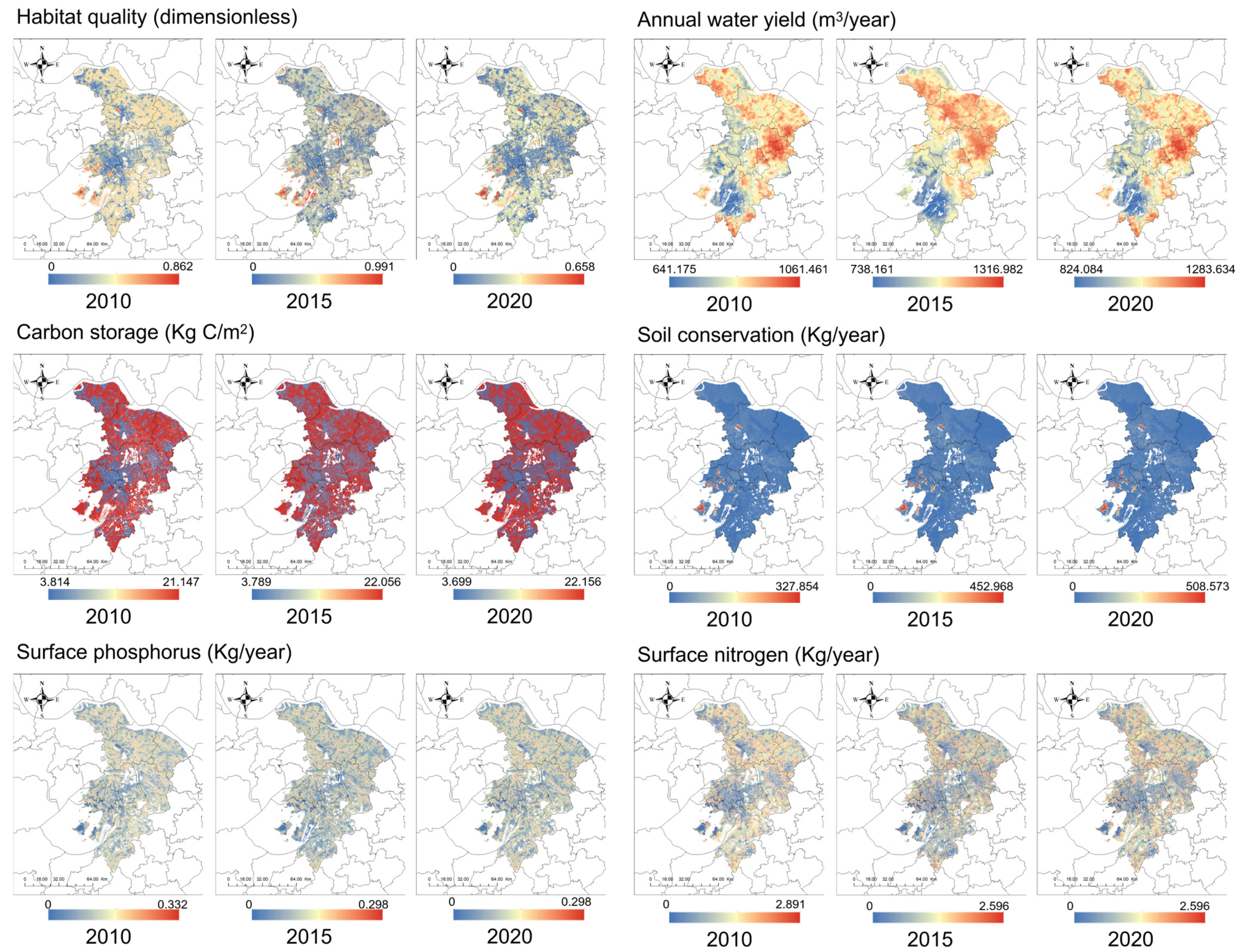
3.1. The Calculation of Supporting and Regulating ESV Based on the inVEST Model

In this study, the total ESV is estimated using the inVEST model combined with the entropy weight method (EWM) by quantifying the information entropy of indicators, thereby objectively reducing the weights of low-variability (highly redundant) indicators. The inVEST model is a widely used ESV evaluation tool based on the Physical Quantity Method [27], which is known for its accuracy in calculating specific types of ESV [28]. The entropy weight method is an objective weighting approach that determines the weight of different indicators based on their information entropy, allowing for a fair and objective calculation of the total ecosystem service value [29]. This effectively compensates for the inVEST model’s inability to directly estimate the total value of ecosystem services. Five modules were used in this study, including annual water yield, carbon storage, habitat quality, sediment delivery ratio, and nutrient delivery ratio.

(1)

Habitat quality

The habitat quality module of inVEST computes the goodness of biodiversity service based on the sensitivity of landscape types and the intensity of external threats [30]. This module requires LULC maps, habitat types and sensitivity levels, threat source types and levels, and the spatial relationship between threat sources and habitats. The calculation results in a habitat quality range of 0–1. The higher the value, the greater the habitat quality of the region. The specific calculation formula is as follows:

$$Q_{xj}=H_j·\left(1-D_{xj}^z/(D_{xj}^z-k^z)\right)$$

(1)

In Formula (1), Q_xj represents the habitat quality of j type land use in grid x; H_j represents the habitat suitability of J type land use; D_xj represents the impact level of the income threat source of J type land use in grid x; and k is the scale constant. D_xj is computed as follows:

$$D_{xj}={\displaystyle \sum _{r=1}^R{\displaystyle \sum _{y=1}^{Y_r}\left(W_r/\left({\displaystyle \sum _{r=1}^R{W}_r}\right)\right)}}·r_j{i}_{rxy}{\beta }_x{S}_{jr}$$

(2)

In Formula (2), R is the impact value of habitat pressure; R is the corresponding threat source; Y_r is the grid number of the threat source r; Y_r is the number of grids occupied by the threat source r; W_r is the influence weight of the threat source r, and the value range is 0–1; i_rxy is the impact of the threat source r, on the habitat (exponential or linear); β_x is the level of habitat anti-interference; and S_jr is the relative sensitivity of different habitats to each threat source r.

(2)

Annual water yield

The annual water yield module of inVEST is based on the water heat coupling balance theory proposed by Budyko [31]. By inputting the evaporation and precipitation data for each grid in the study area, the annual water yield for the study area is finally obtained. The calculation formula is as follows:

$$Y\left(x\right)=\left(1-AET\left(x\right)/P\left(x\right)\right)·P\left(x\right)$$

(3)

In Equation (3), AET(x) represents the actual annual evaporation of the grid x, and P(x) represents the annual precipitation of the grid x.

(3)

Carbon storage

The carbon storage calculation in the inVEST model is based on the land use type classification of the study area, combined with the carbon density values corresponding to the four basic carbon pools of each land use type [32]. In this study, the land use type classification is derived from LULC maps generated by the RF algorithm, while the carbon pools are referenced from established data in previous studies. The calculation accuracy of the results largely depends on the accuracy of the LULC diagram, so the LULC diagram must be strictly evaluated [33]. The four basic carbon pools include the above-ground carbon pool (carbon in all living plant materials above the soil), the underground carbon pool (carbon in plant living root systems), the soil carbon pool (organic carbon in mineral soil), and the dead organic carbon pool (carbon in litter, dead wood, and garbage). The model summarizes the carbon stored in these carbon pools according to land use classification [34]. The calculation principle is as follows:

$$C_T=C_a+C_b+C_s+C_d$$

(4)

In Formula (4), C_T is the total carbon storage amount (t/hm²), and C_a, C_b, C_s, and C_d are above-ground carbon storage, underground carbon storage, soil carbon storage, and dead organic carbon storage, respectively.

(4)

Sediment delivery ratio

In this research, soil retention is computed using the sediment delivery ratio module of inVEST, which is based on the improved universal soil loss equation (USLE) theory [35]. First, compute the soil erosion sediment in each grid cell, and then compute the sediment delivery ratio (SDR), which is the proportion of sediment reaching the outlet of the catchment area to the total amount of soil erosion sediment in the upstream. Then, compute the total annual soil erosion in each grid unit using the following calculation formula:

$$usl{e}_i=R_i·K_i·L{S}_i·C_i·P_i$$

(5)

In Equation (5), R_i represents the precipitation erosion factor, K_i represents the soil erosion factor, LS_i represents the slope length factor, C_i represents the vegetation coverage rate and crop management factor, and P_i represents the water and soil conservation measurement factor.

(5)

Nutrient delivery ratio

In this research, the pollutant absorption computed using the nutrient (nitrogen and phosphorus) delivery ratio (NDR) module in inVEST, which is based on LULC maps, precipitation, vegetation interception, runoff, and other factors, computes the nutrient content in each grid and summarizes the nutrient yield and absorption of each grid cell [36]. The formula is as follows:

$$AL{V}_x=HS{S}_x·po{l}_x$$

(6)

In Equation (6), ALV_x is the output value of the affected material adjusted by the grid, x, pol_x is the output coefficient of the grid, HSS_x is the hydrological sensitivity score of the grid, x.

3.2. Entropy Weight Method

The entropy weight method (EWM) is an objective weighting method based on information entropy theory. There are interactive effects between ESVs, and EWM effectively avoids duplicate calculations of service functions through a weighting mechanism, ensuring that the contribution of each service is independently estimated. This method avoids the redundancy that may arise from simple linear estimation [37] and effectively solves the problem of high correlation between indicators. Its principle and formula are as follows:

$$Y_{ij}=(x_{ij}-x_{j\min })/(x_{j\max }-x_{j\min })$$

(7)

$$Y_{ij}=(x_{j\max }-x_{ij})/(x_{j\max }-x_{j\min })$$

(8)

Before EWM calculation, the data need to be standardized. In these datasets, habitat quality, annual yield, carbon storage, and soil retention should be positively standardized, as shown in Formula (7), while the contents of nitrogen and phosphorus should be negatively standardized, as shown in Equation (8). In Equations (7) and (8), Y_ij is the standardized value of x_ij; x_ij is the j th value of the i th index; and x_jmax and x_jmin are the maximum and minimum values of the j th index.

$$p_{ij}=Y_{ij}/{\displaystyle \sum _{i=1}^n{Y}_{ij}}(i=1,2,\dots ,n;j=1,2,\dots ,m)$$

(9)

The second step is to find the ratio of the overall total value of each index. In Formula (9), if there are m indicators and each index has n group of data, it is recorded as Y_ij. Then, the weight of the total value of each group is computed.

$$Ej=-\ln {(n)}^{-1}{\displaystyle \sum _{i=1}^n{p}_{ij}\ln }{p}_{ij}$$

(10)

In the third step, the information entropy is obtained. In Formula (10), E_j is the information entropy of the index j, and p_ij is the proportion of the i th data in the j th index. When p_ij = 0, the information entropy is E_ij = 0.

$$Hi=1-E_i$$

(11)

In the fourth step, compute the difference coefficient, H_i, for the i th index using Formula (11) as follows:

$$w_i=H_i/{\displaystyle \sum _{n=1}^n{H}_i;\left(0\le w_i\le 1\right)},{\displaystyle \sum _{i=1}^n{w}_i=1}$$

(12)

Finally, in Formula (12), the exponential difference coefficient, H_i, is normalized to compute the exponential weight, w_i.

3.3. Feature Importance Calculation Based on the XGBoost Algorithm

Extreme Gradient Boosting (XGBoost) is a decision tree algorithm based on the gradient boosting framework. It integrates multiple weak learners into a strong model, retains influential features, and eliminates less important ones. XGBoost is capable of simultaneously modeling both linear and nonlinear relationships between independent and dependent variables. XGBoost has demonstrated excellent performance in many applications, particularly in identifying important features that influence model predictions and decision-making [38]. The feature importance is calculated using two key indices as follows:

(1) Coverage: This metric reflects the frequency with which a feature is used as a split point in all decision trees. The more frequently a feature is used, the more important it is considered in the model. The formula for calculating coverage is as follows:

$$Coverag{e}_j=[{\displaystyle \sum i=w^{n}I\left(j,T_i\right)}]/n$$

(13)

In Equation (13), I(j,T_i) is an indicator function where the feature j, is used as a split point in the decision tree, T_i is the number of decision trees, w is the weight of split point in the decision tree.

(2) Gain: This metric reflects the contribution of features to the splits in decision trees. The XGBoost algorithm evaluates the gain at each split point, measuring the improvement in model accuracy due to the split. The formula for calculating gain is as follows:

$$Gainj=[{\displaystyle \sum i=\Delta \backslash loss\left(T_i\right)}]/h$$

(14)

In Equation (14), Δ\loss(T_i) is the decrease in the objective function after adding the decision tree, T_i, and h is the depth of the decision tree.

(3) Feature importance is a comprehensive reflection of coverage and gain, which can usually be computed using Formula (15) as follows:

$$Importanc{e}_j=Coverag{e}_j\times Gai{n}_j$$

(15)

3.4. Principal Component Analysis

Principal Component Analysis (PCA) is a widely used statistical method for dimensionality reduction and feature extraction. The core goal of PCA is to transform multidimensional variables into a set of new and comprehensive indicators (principal components) with linear independence through orthogonal transformation on the premise of preserving the main information of the data [39]. This method simplifies the complexity of the data by preserving the maximum variance of the data after dimension reduction and minimizing the loss of information. The PCA method can be expressed as follows:

$$P{C}_i=l_{1i}{X}_1+l_{2i}{X}_2+\dots +l_{ni}{X}_n$$

(16)

In Formula (16), PC_i is the i th principal component, and l_ij is the loading of the observed variable, X_j (i, j = 1, 2, …, n).

3.5. GWR Method

Geographically Weighted Regression (GWR) is a spatial statistical method designed to address spatial heterogeneity and non-stationarity. The GWR model accounts for spatial variation in the relationship between variables [40]. By introducing kernel functions and bandwidth parameters, GWR overcomes the limitation of assuming constant global parameters in traditional regression models, allowing regression coefficients to vary spatially and revealing the non-stationary characteristics of spatial data.

$$Y_i={\beta }_0\left(u_i,v_i\right)+{\displaystyle \sum _{k=1}^p{\beta }_k}\left(u_i,v_i\right)X_{ik}+{\epsilon }_i$$

(17)

In Equation (17), i is the serial number of the sample point (i = 1, 2, …, n), Y_i is the dependent variable, X_ik is the k th independent variable, (u_i, v_i) is the coordinate of the sampling point i, β_k (u_i, v_i) is the regression parameter of the k th predictor variable, and βuv (u_i, v_i) and ε_i are the regression constant and random error of the sample point, i, respectively. GWR is a function estimation method that takes the function value of each independent variable for each geographical location, i. In this paper, a 500 × 500 grid was built in the study area to extract the data. Coarser grids (e.g., >1 km²) would oversmooth geographic gradients, causing the distortion of local regression coefficients. In addition, finer grids (e.g., <200 m²) would increase data sparsity, amplify micro-scale noise, and reduce the interpretability of the results.

3.6. Overall Research Process

The methodology of this study consists of four main steps as follows:

(1)

Data collection and pre-processing: Collecting remote sensing images and driving factor data, and then applying the RF algorithm to compute the LULC maps for 2010 to 2020.

(2)

The computation of LULC maps: Land use classification processes using the random forest algorithm based on remote sensing images from Landsat-7 surface reflectance data.

(3)

Screening driving factors: Based on the feature importance results from the XGBoost algorithm, weak explanatory factors are removed, and strong ones are retained. The remaining factors are then subjected to PCA for dimensionality reduction, transforming the original correlated factors into three principal components (PCs) with linear independence.

(4)

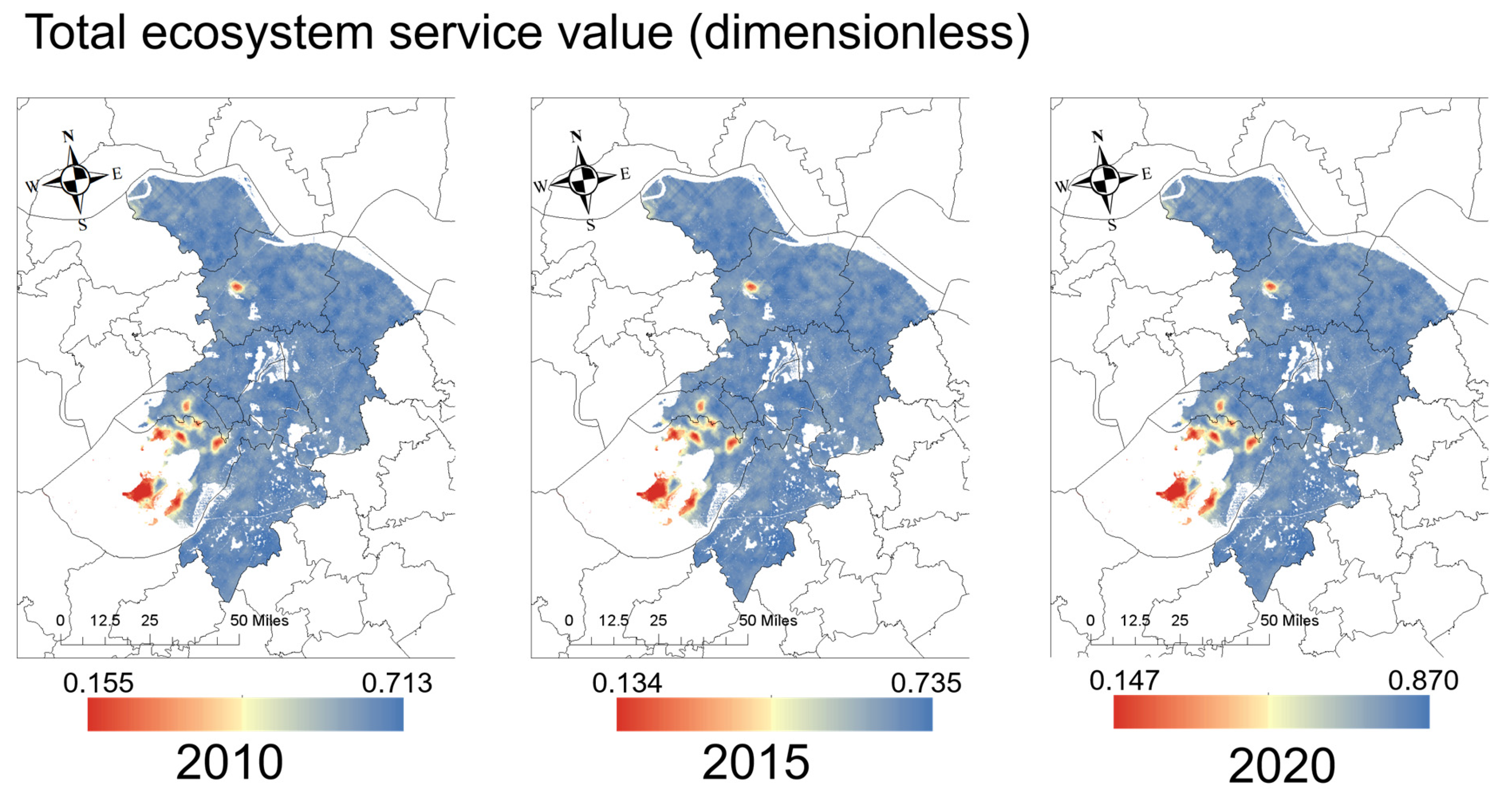
Computing the total value of ecosystem services: Using the inVEST model to compute six ecosystem service value (ESV) indicators, assign weights to each indicator through EWM, and then calculate the total value and its spatial distribution for the period of 2010–2020.

(5)

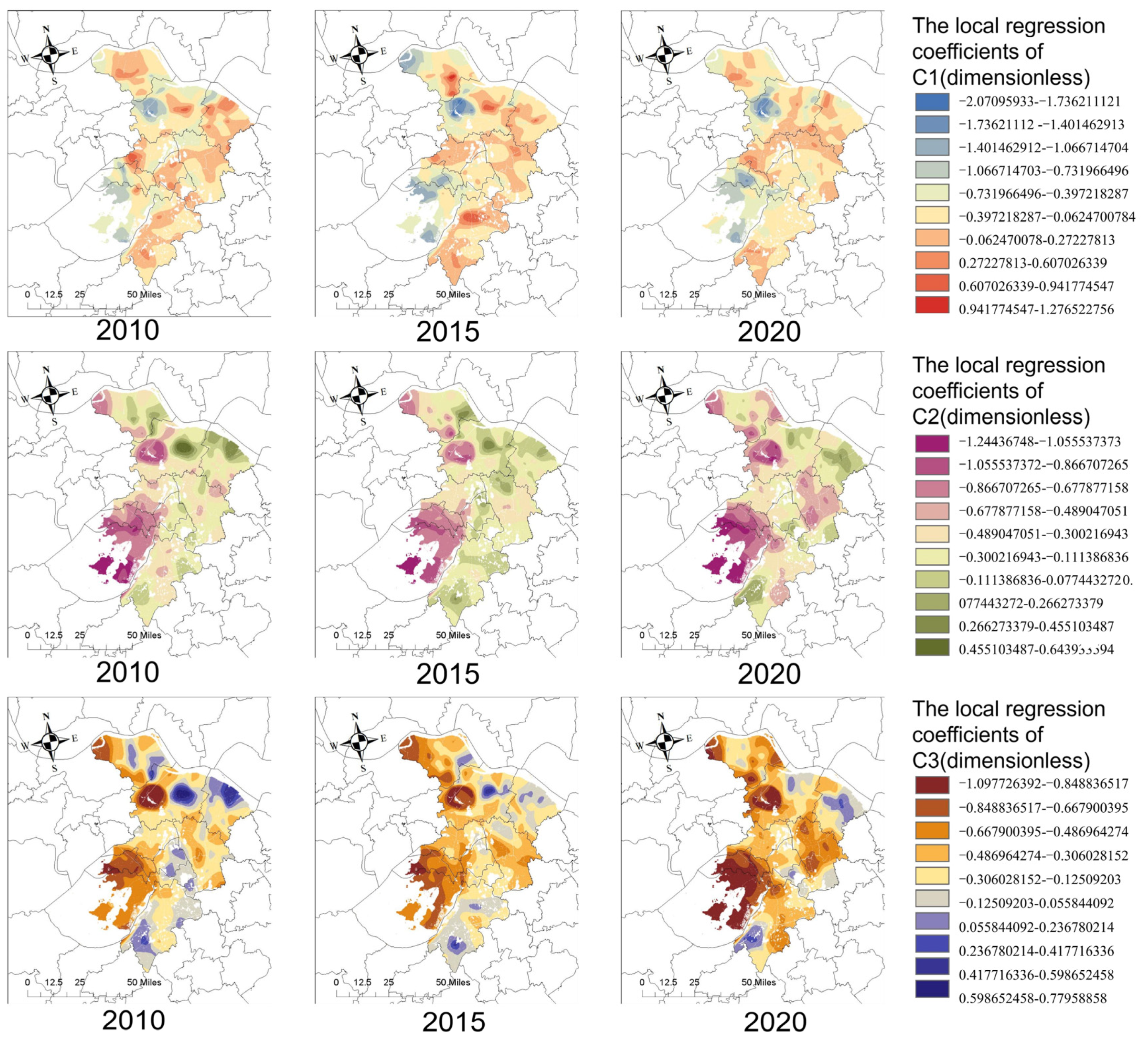
Exploring the influencing mechanism: Using the principal components as independent variables and the total ESV as the dependent variable, GWR is applied to determine the spatial and temporal variations in the regression coefficients. The overall research framework is shown in Figure 6.

4. Result Analysis

4.1. Entropy Weight Method Weight Distribution and Total Value of ESV Calculation Results

Before calculating the total ESV value and screening the driving factors, a correlation matrix needs to be constructed to explore the relationships between the ESV indicators and between the driving factors. The results, as shown in Figure 7, reveal a significant correlation both among the ESV indicators and among the driving factors. Therefore, data processing using the EWM and XGBoost algorithms is necessary to effectively reduce redundant information and multicollinearity in the data.

4.2. Entropy Weight Method and ESV Calculation

According to the results of six types of services calculated in the inVEST model, the values for annual water yield, nitrogen absorption, and phosphorus absorption increased. Specifically, annual water yield increased from 890.599 to 1102.385, while the average surface nitrogen content decreased from 0.580 to 0.551, and the surface phosphorus content decreased from 0.0643 to 0.0626. However, habitat quality decreased from 0.210 to 0.168. The main reason for this phenomenon is that policy implementation is not in place. First, according to the General Planning of Land and Space of Suzhou City (2021–2035), the urban development boundary will be controlled within 2651.83 square kilometers by 2035. However, the actual development boundary rapidly extended to the Taihu Lake coast from 2010 to 2020, resulting in the reduction of ecological space. In addition, although the plan proposes to “strictly abide by the ecological protection red line”, it often makes way for industrial projects by “adjusting the ecological space control area handling procedures”. For example, the 2024 policy allows for simplified approval of “ecological red line area projects that do not involve new construction land”, indirectly reducing the intensity of ecological protection [41]. The values for carbon storage and soil conservation services showed no significant variation during the study period (Figure 8).

The entropy weight method (EWM) was used to obtain the final weights for each indicator. The final weights are as follows: annual water yield 1.5%, soil retention 45.5%, phosphorus absorption 12.3%, nitrogen absorption 10.2%, habitat quality 27.1%, and carbon storage 3.2%. The spatial distribution of ESV in 2010, 2015, and 2020 is shown in Figure 9. According to the final distribution maps of the total value of ecosystem services from 2010 to 2020, the mean value was 0.227 in 2010, 0.209 in 2015, and 0.252 in 2020, representing an overall increase of 9.92%. This reflects a process of values falling first and then rising. From a spatial distribution perspective, the Global Moran’s I index of the total value was 0.325, 0.476, and 0.489 in 2010, 2015, and 2020, respectively. As the Moran’s I index increases, the spatial clustering of ESV values strengthens, indicating a more uneven distribution and potentially higher ecological risks in the study area.

4.3. Results of the XGBoost Algorithm

The feature importance calculation based on the XGBoost algorithm is discussed in this study. For the parameter settings of the model, feature importance analysis requires stable and interpretable models. The model must balance model generalization with feature interaction capture (via controlled tree depth) while ensuring convergence speed and mitigating overfitting risks (via appropriate learning rate selection). This article refers to previous research and sets parameters based on the actual situation of the research data. The algorithm was constructed using R Studio 4.3.3 software, with the maximum depth of the tree set to 4, the learning rate set to 0.3, and the number of boosting rounds set to 50. Finally, this study refers to past research experience and only retains the top 80% of the factors in terms of their total feature importance. This step eliminated six weak explanatory factors, including LAI, Contag, Pd, sidi, siei, and split, leaving 31 factors remaining.

The retained 31 factors are potentially correlated and contain redundant information, according to the results of previous correlation analysis. Therefore, additional measures are necessary to address the multicollinearity among the retained driving factors. To address the multicollinearity among the retained driving factors, Principal Component Analysis (PCA) and Variance Inflation Factor (VIF) are applied for linear dimensionality reduction. PCA reduces the feature space by extracting principal components (the directions of highest variance) while retaining most of the information in the data. By combining redundant features into fewer principal components, the model’s complexity is simplified. In this study, prior to applying PCA, VIF is used to detect multicollinearity as a widely used method for assessing the degree of correlation between features. A higher VIF indicates a stronger correlation between a given factor and other factors. Generally, if the VIF is greater than 5, it indicates the possibility of collinearity. Under relaxed conditions, the VIF is greater than 10. In this study [42], the criterion of VIF less than 10 was adopted. On one hand, the number of retained features is relatively large, and relaxing the criterion can avoid over-screening and loss of important features [43]. On the other hand, this study adopts the GWR model, which focuses on spatial heterogeneity and is not sensitive to collinearity like the global linear regression model, which allows for the appropriate relaxation of the VIF standard [44,45]. Therefore, when the VIF exceeds 10, it signals a high degree of multicollinearity, which can cause instability in the model’s estimates and negatively affect both its interpretability and predictive power. In this paper, nine factors with linear independence were selected through VIF collinearity screening (

Table 2. Factors selected via VIF collinearity screening.

Coefficients
Unstandardized Coefficients			Standardized Coefficients			Collinearity Statistics
Model	B	Std. Error	Beta	t	Sig.	Tolerance	VIF
(Constant)	1.094	0.007		150.073	<0.001
Slope	−0.496	0.006	−0.445	−85.964	<0.001	0.434	2.304
Elevation	−0.44	0.009	−0.269	−51.593	<0.001	0.429	2.332
NPP	−0.065	0.003	−0.087	−20.653	<0.001	0.648	1.543
Airtemperature	−0.158	0.003	−0.442	−49.589	<0.001	0.146	6.833
Humidity	0.162	0.003	0.435	53.388	<0.001	0.175	5.726
Ndvi	0.061	0.003	0.077	20.243	<0.001	0.809	1.236
Iji	0.033	0.003	0.042	10.68	<0.001	0.752	1.329
Windspeed	0.017	0.002	0.034	8.179	<0.001	0.673	1.486
Aridity	0.017	0.002	0.036	7.772	<0.001	0.551	1.816

).

The purpose of PCA is to further reduce the dimensionality of complex data structures and extract the most significant features. The focus is on identifying the most influential loadings (both positive and negative) in each principal component. A loading represents the weight of the original variable in the component, with the largest loadings typically highlighting the key factors that influence the component. While other secondary loadings may offer some explanatory insights, excessive emphasis on them can increase complexity, obscure the dominant factors, and reduce interpretability. Based on the factor loadings of the principal components, they are labeled as C1, C2, and C3 (

Table 3. Principal components and their cumulative variance contribution rate.

Total Variance Explained
Component	Initial Eigenvalues			Extraction Sums of Squared Loadingings
	Total	% of Variance	Cumulative %	Total	% of Variance	Cumulative %
C1	2.679	29.762	29.762	2.679	29.762	29.762
C2	2.23	24.778	54.54	2.23	24.778	54.54
C3	1.31	14.552	69.092	1.31	14.552	69.092

and

Table 4. Various driving factors loading onto different principal components.

Component Matrix
Factors	Component
	1	2	3
Slope	0.275	0.711	0.494
Dem	0.285	0.734	0.415
NPP	0.413	0.513	−0.488
Airtemperature	0.907	−0.293	−0.037
Humidity	0.869	−0.314	0.008
Ndvi	−0.004	−0.549	0.463
Iji	−0.123	−0.611	0.406
Windspeed	−0.576	−0.018	−0.412
Aridity	−0.653	0.252	0.324

). These three principal components explain 69.092% of the cumulative variance, demonstrating their significant explanatory power and effectively capturing the main driving factors of the original data.

4.4. GWR Fitting Results

Before applying geographically weighted regression (GWR), the Global Moran’s I index is used to evaluate the spatial autocorrelation of the principal components (C1 to C3). If no spatial autocorrelation is detected, GWR will not provide more reliable results than ordinary least squares regression (OLS) [46]. Finally, the Global Moran’s I result indicates significant spatial autocorrelation for the three principal components (

Table 5. Analysis of the spatial autocorrelation of the principal components.

Principal Components	Moran’s I	Z Value		p Value
	2010	2015	2020	2010	2015	2020	2010	2015	2020
C1	0.971041	0.992501	0.961092	587.5	475.6	476.9	0.000	0.000	0.000
C2	0.988701	0.967741	0.983406	598.2	475.7	474.7	0.000	0.000	0.000
C3	0.978791	0.975082	0.992171	611.5	477.2	462.2	0.000	0.000	0.000

).

After verifying the spatial autocorrelation of the principal components (C1 to C3), the total ecosystem service value was treated as the dependent variable, and the principal components were used as the independent variables. The GWR method was then applied to calculate the local regression coefficients for the years 2010 to 2020. The final results were compared with those obtained using the ordinary least squares (OLS) method. In this study, the Coefficient of Determination (R²) and the Corrected Akaike Information Criterion (AICc) were used to assess the goodness of fit between the two regression methods. R² values range from 0 to 1, with values closer to 1 indicating a better model fit, suggesting that the independent variables can more effectively explain the variations in the dependent variable. A smaller AICc value indicates a more efficient model that better aligns with the observed data [47,48].

In 2010, the R² of GWR was 0.531, which is higher than OLS’s 0.367, and the AICc value was 24,714.471, which is lower than the OLS value of 27,783.408. In 2015, the R² of GWR was 0.632, which is higher than OLS’s 0.416, and the AICc value was 21,962.963, which is lower than OLS’s 26,837.417. In 2020, the R² of GWR was 0.657, which is higher than OLS’s 0.459, and the AICc value was 21,004.868, which is lower than OLS’s 25,829.790. The comparison results showed that the goodness of fit for GWR was consistently higher than that for OLS.

5. Discussion

After GWR analysis, the temporal–spatial distribution of local regression coefficients for the principal components C1 to C3 is shown in Figure 10, and this paper uses different colors to represent the local regression coefficients’ high and low degrees. Based on the spatiotemporal analysis of score distributions and the loadings of the three principal components, we found that C1 is primarily associated with climate, C2 is primarily associated with topography and landscape, and C3 is primarily associated with topography and vegetation. Notably, C1 exhibited no significant variation between 2010 and 2020, while both C2 and C3 displayed significant changes during this period. This indicates that topographic factors are the most dynamic among the various influencing mechanisms.

5.1. Air Temperature and Aridity’s Influencing Mechanism on Ecosystem Services

Principal Component C1 exhibits the highest positive loading for air temperature and the highest negative loading for aridity, both of which are climate-related factors. The positive value of C1 reflects a humid and warm climatic condition. The negative value of C1 reflects a dry and cool climatic condition. From 2010 to 2020, the regression coefficients of C1 in Suzhou City have generally been negative, particularly in high-altitude forest lands, where high temperatures and humid climate conditions have a detrimental effect on ecosystem services. However, in some high-density urban built-up areas, the effect has been positive (Figure 10).

In high-altitude forest areas and most flatland areas (the whole study area, except for the Xiangcheng, central Zhangjiagang, northern Kunshan, central Changshu, and central Wujiang Districts), C1 plays a negative role. Although in other studies, higher temperatures are sometimes regarded as a factor conducive to plant growth, this paper found that in the high-altitude forests of Suzhou [49], high temperatures increase the respiration rate of trees, inhibiting their growth, and are often accompanied by high rainfall and steep slopes. Dry environments are beneficial for soil conservation [50,51] because they reduce runoff erosion and nutrient loss. Simultaneously, high temperatures and humidity can boost soil microbial activity, accelerating the decomposition of organic matter, which diminishes organic matter accumulation and reduces soil carbon storage capacity. In flatland areas [52,53], the combination of high temperatures and high humidity has negative effects on soil carbon storage. High temperatures speed up the decomposition of soil organic matter, while high humidity leads to nutrient loss, ultimately decreasing soil organic carbon storage [54,55]. Furthermore, high temperatures and high humidity typically damage soil structure, resulting in reduced soil stability. High temperatures cause soil moisture to evaporate, while high humidity leads to excessive surface moisture, which can easily result in soil erosion and nutrient loss.

In a few high-density built-up areas (the Xiangcheng, central Zhangjiagang, northern Kunshan, central Changshu, and central Wujiang Districts) where C1 plays a positive role, the growth of green spaces and vegetation in the city accelerates in humid and high-temperature environments. This conclusion is contrary to the findings from high-altitude forests and flatlands and some previous studies. Compared with the wild, the vegetation in the Suzhou urban area shows better adaptability. When greening the Suzhou urban area, plants with strong adaptability and significant ecological benefits are often selected. For example, Jasminum nudiflorum, Koelreuteria paniculata, Magnolia grandiflora, and other heat- and moisture-resistant species can still grow well in high-temperature and high-humidity environments [56]. In addition, in high-density built-up areas (such as Xiangcheng District, Zhangjiagang City Center, etc.), the high-temperature and -humidity environment can promote the rapid growth of vegetation, increase the area of urban green space, and improve the environment. Fast-growing vegetation can not only absorb surface runoff but also enhance soil conservation capacity, thereby improving ecosystem services as a whole [57,58]. This rapid growth can not only increase urban green space and improve habitat quality but also help absorb surface runoff and enhance soil conservation capacity.

In terms of spatiotemporal changes, the regression coefficient region of C1 exhibited a significant change between 2010 and 2020, and C1’s positively impacted area decreased by 195.51 km².

5.2. Elevation and Landscape Pattern Influencing Mechanism on Ecosystem Services

Principal Component C2 exhibits the highest positive loading for elevation and the highest negative loading for the landscape pattern index (IJI), which are topographical and landscape pattern-related factors. The IJI is used to describe the spatial allocation and distribution of different land types within a unit area. Regions with a high IJI usually indicate a high degree of landscape fragmentation, a more complex landscape structure, and greater heterogeneity. The positive value of C2 reflects higher elevation and a simpler landscape structure with less fragmentation, while the negative value of C2 reflects lower elevation and a more complex landscape structure with greater fragmentation. From 2010 to 2020, the local regression coefficients for C2 in Suzhou City have predominantly been negative. High-altitude areas with a high IJI value tend to have a negative impact on ecosystem services, particularly in high-altitude forest areas and high-density urban built-up areas. A positive effect of C2 was only observed in a few agricultural areas (Figure 10).

In high-altitude forest areas and urban built-up areas (including Huqiu, Kunshan, western Changshu, western Wuzhong, and the southern, eastern, and western Zhangjiagang Districts), C2 exerts a negative influence. High elevation often leads to steeper slopes and increased rainfall, which exacerbate runoff erosion and reduce the soil conservation and carbon sequestration capacity of forests [59]. In urban areas, a higher IJI indicates greater landscape fragmentation, which worsens pollutant dispersion and diminishes the connectivity of green spaces, contributing to habitat degradation. In forested regions, fragmentation lowers biodiversity, increases ecological pressure, and significantly reduces ecosystem services such as carbon storage, water conservation, and habitat quality [60,61]. The abovementioned conclusions are consistent with previous major studies.

In contrast, in certain agricultural areas where C2 has a positive effect (including the northern Changshu, eastern Taicang, and southern Wujiang Districts), the high elevation reduces pollutant input in irrigation water, decreases heavy metal contamination in the soil, and enhances soil nutrient levels, all of which benefit plant growth [62,63]. Additionally, in these agricultural areas, a high IJI value indicates that there are more high-quality habitat patches, enhancing habitat diversity and quality, as well as improving soil fertility. These conclusions are consistent with certain previous studies.

Regarding spatiotemporal changes, the C2 regression coefficient exhibited significant regional variations between 2010 and 2020. Although only 41.46 km² of C2’s negatively impacted area increased, there was a noticeable increase in the degree of negative impact in these areas, particularly in Kunshan. During this period, Kunshan underwent a large-scale conversion of farmland into built-up areas. Kunshan also established several economic development zones that occupied large areas of farmland. Additionally, to meet the rapidly growing urban population’s needs, Kunshan undertook extensive residential and infrastructure construction on the city outskirts. Due to these land use changes, farmland was largely replaced by impervious surfaces, amplifying the negative impact of C2 in the region.

5.3. Slope and NPP’s Influencing Mechanism on Ecosystem Services

Principal Component C3 exhibits the highest positive loading for slope and the highest negative loading for net primary productivity (NPP), which are topographical and vegetation-related factors. The positive value of C3 reflects steeper terrain and lower plant biomass production, while the negative value of C3 indicates smoother terrain and higher plant productivity. From 2010 to 2020, the local regression coefficients for C3 in Suzhou City were predominantly negative, with a positive effect observed only in certain agricultural areas. The negative impact was particularly evident in high-altitude forest areas and urban built-up areas (Figure 10).

In areas where C3 has a negative impact (the whole study area except for the northern Changshu, central and eastern Taicang, and southern Wuzhong Districts), lower NPP and steeper terrain have negative impacts on the ESV, which is consistent with the conclusions of most studies. Lower NPP indicates poor plant productivity. In high-altitude forestlands, limited plant growth, combined with steep terrain, can lead to soil erosion and a decline in soil nutrients [64], thereby reducing ecosystem services such as carbon storage, soil conservation, and habitat quality. In urban built-up areas, dense buildings and impervious surfaces result in poor soil permeability. Steep slopes and insufficient vegetation further exacerbate runoff pollution and soil erosion, which in turn reduce habitat quality and annual water yield [65,66].

In just a few agricultural areas where C3 plays a positive role (the northern Changshu, central and eastern Taicang, and southern Wuzhong Districts), steeper slopes are conducive to drainage [67]. Certain slopes can significantly reduce soil erosion and increase soil water conservation capacity. This conclusion is consistent with previous studies. This type of terrain helps preserve soil fertility and creates a favorable environment for plant growth [68].

Regarding spatiotemporal changes, the local regression coefficients of C2 exhibited significant regional variation between 2010 and 2020. The area negatively impacted by C2 increased by 414.14 km², with a noticeable increase in areas impacted. This increase is primarily linked to the pace of urbanization, which was particularly evident during this period as urban construction land expanded significantly. The growth of construction land was concentrated in urban and surrounding areas, precisely where the negative impact of C2 expanded. For example, in the Suzhou Industrial Park District, much of the original farmland was replaced by modern industrial and residential facilities. This trend was especially pronounced in the county-level cities of Suzhou, like Kunshan, where agricultural land steadily decreased while built-up areas expanded significantly during this period.

5.4. UGSS Planning Optimization Based on the Analysis

In this study, through the spatiotemporal changes in the total value of ecosystem services, as well as the influencing mechanisms of driving factors based on the distribution of local regression coefficients obtained using the XGBoost-GWR method, UGSS planning is proposed as follows:

(1)

Enhance Ecological Protection and Restoration: To address the uneven distribution of ecosystem services, Suzhou should enhance ecological protection and restoration. For high-density urban cores (like the Xiangcheng, central Zhangjiagang, northern Kunshan, central Changshu, and central Wujiang Districts), targeted vegetation enhancements should be implemented by developing pocket parks (minimum size: 0.5 ha) and urban forests (≥30% native tree cover) in areas with limited green space access (within a <500 m radius from residential zones), prioritizing native species with high carbon sequestration and pollution absorption. This approach aligns with the success of aquatic plant restoration, such as at Ziwei Cultural Park in Suzhou, where native species improved water quality from Grade V to III [69].

(2)

Improve Green Space Connectivity and Diversity: For suburban agricultural areas (like the northern Changshu, eastern Taicang, and southern Wujiang Districts), green corridors should be established (with a minimum width of 100 m) to connect fragmented high-quality habitat landscapes and increase diversity while integrating diverse vegetation layers (tree canopy, shrubs, ground cover) to enhance biodiversity. These measures will help connect fragmented green spaces, creating a network that boosts the overall value of ecosystem services. This approach has been successfully verified in Yancheng, Jiangsu Province, where it enhanced ecological connectivity by 20%.

(3)

Strengthen Ecological Barriers and Hydrological Regulation: In urban built-up areas, permeable surfaces should be increased, and impervious surface expansion should be limited to <25% in new developments. In areas of industrial concentration, pollution buffers should be implemented, and 500 m green buffers should be established around high-pollution industries. Through these measures, the diffusion of pollutants around industrial and high-density urban areas can be reduced [70].

(4)

Ecological Restoration and Adaptive Land Use Planning: Soil remediation should be implemented in degraded areas, increasing multifunctional parks in old urban and industrial areas, which can improve water quality. At the same time, soil can be remediated using plants and microorganisms, particularly by planting pollution-tolerant species (such as legumes) [71], which can absorb heavy metals and pollutants, promote the degradation of harmful substances, increase biodiversity, and provide recreational spaces for residents.

(5)

Additionally, establishing an ecological monitoring system to track soil quality, water quality, and vegetation growth in real time helps assess the effectiveness of restoration efforts. By using GIS and remote sensing technologies, continuous monitoring of urban green space changes allows for the evaluation of the impact of different land uses on ecological restoration and the optimization of strategies based on data.

5.5. Limitations and Prospects

This study, while offering insights into the ESV of Suzhou’s UGSS, provides a research perspective that balances global nonlinear dynamics with local spatial heterogeneity, offering a more comprehensive and nuanced understanding of the underlying ecological processes and their regional variations. However, there are still several limitations that need to be addressed.

Firstly, the use of the inVEST model for ESV estimation introduces a dependence on the quality and completeness of the input data. It is sensitive to data resolution and input accuracy, and the input data can be highly variable across different regions, which can lead to deviations in the final calculation. Additionally, the model’s assumptions may not fully capture local ecological dynamics. In addition, the spatial resolution of input data, such as land use/land cover maps or climate data, may also limit the model’s capacity to reflect fine-grained ecological processes. To improve future studies, the integration of higher-resolution remote sensing data and hybrid modeling approaches could be explored to refine ESV estimations and capture more localized ecological variations.

Secondly, while the combination of XGBoost and GWR enables the modeling of spatial heterogeneity and nonlinearity, it does not fully address the complexities of causal relationships between driving factors and ESV. XGBoost’s feature selection and regularization techniques are effective in reducing overfitting but may not fully uncover the underlying interactions between different factors. Additionally, GWR helps capture local variations, but the model’s performance can be sensitive to bandwidth choice and may overlook certain non-local interactions that could be important at larger spatial scales. As such, the dual optimization approach provides valuable insights but still requires further refinement to better handle the intricacies of spatially variable ecological processes and multilevel drivers.

Thirdly, this study primarily focuses on a macro-scale analysis, examining the ESV of UGSS within Suzhou’s administrative boundaries. While this approach is useful for identifying broad patterns and informing urban-scale planning, it may overlook more localized ecological nuances. On a micro-scale, such as specific green space types (e.g., parks or forests), more detailed, site-specific data are necessary to refine models and provide actionable, context-sensitive recommendations. Future research should focus on more granular data collection and analysis, particularly for urban green spaces with varying ecological functions, to improve planning and management strategies at the neighborhood or park level.

6. Conclusions

In this study, we examined Suzhou—a megacity in the Taihu Lake Basin’s core ecological zone—as a critical case for understanding the ecological impacts of rapid industrialization and urbanization on China’s urban green space system. Our study evaluated the ESV in Suzhou City’s UGSS during 2010–2020 using the inVEST model combined with the EWM, and we examined the influencing mechanisms of key factors based on the XGBoost-GWR framework. The results reveal the ecological challenges posed by rapid urbanization in China, identify common ecological issues faced by cities in the Taihu watershed, and demonstrate the effectiveness of the XGBoost algorithm in improving variable selection in GWR. Based on the analysis results, we draw the following conclusions:

The findings reveal that the spatiotemporal changes in the total value of six ecosystem services, including the ESV of water yield, nitrogen absorption, and phosphorus absorption, showed a significant increase, while habitat quality showed a significant decline. Additionally, the total value of ecosystem services followed a pattern of initial decline followed by recovery. Spatially, we observed an increase in the Global Moran’s I index, indicating a rising aggregation of high and low values, along with growing ecological risks due to uneven distribution. This indicates that the environmental protection policies implemented between 2010 and 2020 had a certain positive effect, increasing the total ESV. However, these policies for ecological environment protection were not comprehensive. For example, some habitat patches in certain areas are still threatened, causing a decline in habitat quality. These situations have led to a more uneven spatial distribution.

Through XGBoost feature importance, combined with PCA analysis, this paper effectively reduced redundant information and screened the driving factors. The key factors include climate, topography, landscape pattern, and vegetation. Among these factors, climate had the most significant impact, with the highest explanatory power in the principal components, with its influencing mechanism exhibiting minimal temporal and spatial variation. In contrast, topography showed significant spatial and temporal variability, with its negatively impacted area increasing by 455.60 km², indicating that it is the most dynamic factor. The changes in the influencing mechanisms of key factors were mainly driven by land use changes, particularly industrial development and urban expansion. In regions such as Kunshan, Wujiang, and Zhangjiagang, the conversion of natural surfaces into impervious surfaces has increased ecological risks such as soil erosion, pollution, and habitat degradation.

Our findings underscore the importance of adopting targeted planning measures for green space systems across different regions of Suzhou City to safeguard ecosystem service values. These insights contribute to a deeper understanding of urban ecosystem services in the cities of the Taihu watershed, offering practical guidance for urban planning and sustainable development strategies. Future research should focus on refining the calculation process, improving the factor selection procedure, further simplifying the calculation of ecosystem service value, and improving the accuracy of the model to improve the reliability and applicability of such models in other urban environments.

References

1. Yang, J.; Guan, Y.; Xia, J.C.; Jin, C.; Li, X. Spatiotemporal variation characteristics of green space ecosystem service value at urban fringes: A case study on Ganjingzi District in Dalian, China. Sci. Total Environ. 2018, 639, 1453–1461. [Google Scholar] [CrossRef] [PubMed]
2. Pinto, L.V.; Inácio, M.; Ferreira CS, S.; Ferreira, A.D.; Pereira, P. Ecosystem services and well-being dimensions related to urban green spaces–A systematic review. Sustain. Cities Soc. 2022, 85, 104072. [Google Scholar] [CrossRef]
3. Xu, H.; Paerl, H.W.; Zhu, G.; Qin, B.; Hall, N.S.; Zhu, M. Long-term nutrient trends and harmful cyanobacterial bloom potential in hypertrophic Lake Taihu, China. Hydrobiologia 2017, 787, 229–242. [Google Scholar] [CrossRef]
4. Zhang, J.; Zhang, J. Countermeasures to Control NPS Pollution in Headwaters of Taihu Lake Basin. In Forestry Measures for Ecologically Controlling Non-Point Source Pollution in Taihu Lake Watershed, China; Springer: Dordrecht, The Netherlands, 2016; pp. 43–54. [Google Scholar]
5. Guo, G.H.; Wu, F.C.; He, H.P.; Zhang, R.Q.; Li, H.X. Screening level ecological risk assessment for synthetic musks in surface water of Lake Taihu, China. Stoch. Environ. Res. Risk Assess. 2013, 27, 111–119. [Google Scholar] [CrossRef]
6. Pernice, R. Verticality and Conflicting Identities in the Contemporary Chinese City: The Urban Development of Suzhou Industrial Park. J. Chin. Archit. Urban. 2021, 3, 1026. [Google Scholar] [CrossRef]
7. Fang, C.; Chen, C.; Zhao, M.; LeGates, R. Integrating urban-rural development (IURD) through governance programmes in China’s Megacities: The Suzhou model. In New Urban Agenda in Asia-Pacific: Governance for Sustainable and Inclusive Cities; Springer: Singapore, 2020; pp. 39–64. [Google Scholar]
8. He, L.; Xie, Z.; Wu, H.; Liu, Z.; Zheng, B.; Wan, W. Exploring the interrelations and driving factors among typical ecosystem services in the Yangtze river economic Belt, China. J. Environ. Manag. 2024, 351, 119794. [Google Scholar] [CrossRef]
9. Wang, H.; Liu, G.; Li, Z.; Zhang, L.; Wang, Z. Processes and driving forces for changing vegetation ecosystem services: Insights from the Shaanxi Province of China. Ecol. Indic. 2020, 112, 106105. [Google Scholar] [CrossRef]
10. Wang, X.; Wu, J.; Liu, Y.; Hai, X.; Shanguan, Z.; Deng, L. Driving factors of ecosystem services and their spatiotemporal change assessment based on land use types in the Loess Plateau. J. Environ. Manag. 2022, 311, 114835. [Google Scholar] [CrossRef]
11. Lyu, R.; Clarke, K.C.; Zhang, J.; Feng, J.; Jia, X.; Li, J. Spatial correlations among ecosystem services and their socio-ecological driving factors: A case study in the city belt along the Yellow River in Ningxia, China. Appl. Geogr. 2019, 108, 64–73. [Google Scholar] [CrossRef]
12. Liu, W.; Zhan, J.; Zhao, F.; Wang, C.; Zhang, F.; Teng, Y.; Chu, X.; Kumi, M.A. Spatio-temporal variations of ecosystem services and their drivers in the Pearl River Delta, China. J. Clean. Prod. 2022, 337, 130466. [Google Scholar] [CrossRef]
13. Gao, J.; Zuo, L. Revealing ecosystem services relationships and their driving factors for five basins of Beijing. J. Geogr. Sci. 2021, 31, 111–129. [Google Scholar] [CrossRef]
14. Geng, T.W.; Chen, H.; Zhang, H.; Shi, Q.Q.; Liu, D. Spatiotemporal evolution of land ecosystem service value its driving factors in Shaanxi province based on, G.W.R. J. Nat. Resour. 2020, 35, 1714–1727. [Google Scholar]
15. Fotheringham, A.S.; Crespo, R.; Yao, J. Geographical and temporal weighted regression (GTWR). Geogr. Anal. 2015, 47, 431–452. [Google Scholar] [CrossRef]
16. Ogunleye, A.; Wang, Q.G. XGBoost model for chronic kidney disease diagnosis. IEEE/ACM Trans. Comput. Biol. Bioinform. 2019, 17, 2131–2140. [Google Scholar] [CrossRef]
17. Wang, X.J. Analysis of problems in urban green space system planning in China. J. For. Res. 2009, 20, 79–82. [Google Scholar] [CrossRef]
18. Heidt, V.; Neef, M. Benefits of urban green space for improving urban climate. In Ecology, Planning, and Management of Urban Forests: International Perspectives; Springer: New York, NY, USA, 2008; pp. 84–96. [Google Scholar]
19. Vadde, K.K.; Wang, J.; Cao, L.; Yuan, T.; McCarthy, A.J.; Sekar, R. Assessment of water quality and identification of pollution risk locations in Tiaoxi River (Taihu Watershed), China. Water 2018, 10, 183. [Google Scholar] [CrossRef]
20. Wu, Z.; Wang, X.; Chen, Y.; Cai, Y.; Deng, J. Assessing river water quality using water quality index in Lake Taihu watershed, China. Sci. Total Environ. 2018, 612, 914–922. [Google Scholar] [CrossRef]
21. Chen, L.; Zhou, S.; Shi, Y.; Wang, C.; Li, B.; Li, Y.; Wu, S. Heavy metals in food crops, soil, and water in the Lihe River Watershed of the Taihu Region and their potential health risks when ingested. Sci. Total Environ. 2018, 615, 141–149. [Google Scholar] [CrossRef]
22. Cai, Y.; Wu, J.; Yimiti, T.; Li, Z.; Yang, X.; Dong, S. The landscape altered the interaction between vegetation and climate in the desert oasis of Hotan River Basin, Xinjiang, China. Ecol. Model. 2024, 491, 110687. [Google Scholar] [CrossRef]
23. Breiman, L. Random Forests. Mach. Learn. 2001, 45, 5–32. [Google Scholar] [CrossRef]
24. Kafy, A.-A.; Saha, M.; Fattah, M.A.; Rahman, M.T.; Duti, B.M.; Rahaman, Z.A.; Bakshi, A.; Kalaivani, S.; Rahaman, S.N.; Sattar, G.S. Integrating forest cover change and carbon storage dynamics: Leveraging Google Earth Engine and InVEST model to inform conservation in hilly regions. Ecol. Indic. 2023, 152, 110374. [Google Scholar] [CrossRef]
25. Pande, C.B.; Srivastava, A.; Moharir, K.N.; Radwan, N.; Mohd Sidek, L.; Alshehri, F.; Pal, S.C.; Tolche, A.D.; Zhran, M. Characterizing land use/land cover change dynamics by an enhanced random forest machine learning model: A Google Earth Engine implementation. Environ. Sci. Eur. 2024, 36, 84. [Google Scholar] [CrossRef]
26. Feizizadeh, B.; Omarzadeh, D.; Kazemi Garajeh, M.; Lakes, T.; Blaschke, T. Machine learning data-driven approaches for land use/cover mapping and trend analysis using Google Earth Engine. J. Environ. Plan. Manag. 2023, 66, 665–697. [Google Scholar] [CrossRef]
27. Cao, Y.; Ma, Y.; Bao, A.; Chang, C.; Liu, T. Evaluation of the water conservation function in the Ili River Delta of Central Asia based on the InVEST model. J. Arid. Land 2023, 15, 1455–1473. [Google Scholar] [CrossRef]
28. Gao, X.; Huang, X.-x.; Chang, S.-h.; Dang, Q.-w.; Wen, R.-y.; Lo, K.; Li, J.; Yan, A. Long-term improvements in water conservation functions at Qilian Mountain National Park, northwest China. J. Mt. Sci. 2023, 20, 2885–2897. [Google Scholar] [CrossRef]
29. Cao, C.; Wei, T.; Xu, S.; Su, F.; Fang, H. Comprehensive evaluation of higher education systems using indicators: PCA and EWM methods. Humanit. Soc. Sci. Commun. 2023, 10, 1–12. [Google Scholar] [CrossRef]
30. He, N.; Guo, W.; Wang, H.; Yu, L.; Cheng, S.; Huang, L.; Jiao, X.; Chen, W.; Zhou, H. Temporal and spatial variations in landscape habitat quality under multiple land-use/land-cover scenarios based on the PLUS-InVEST model in the Yangtze River Basin, China. Land 2023, 12, 1338. [Google Scholar] [CrossRef]
31. Valencia, J.B.; Guryanov, V.V.; Mesa-Diez, J.; Tapasco, J.; Gusarov, A.V. Assessing the Effectiveness of the Use of the InVEST Annual Water Yield Model for the Rivers of Colombia: A Case Study of the Meta River Basin. Water 2023, 15, 1617. [Google Scholar] [CrossRef]
32. Zhao, M.; He, Z.; Du, J.; Chen, L.; Lin, P.; Fang, S. Assessing the effects of ecological engineering on carbon storage by linking the CA-Markov and InVEST models. Ecol. Indic. 2019, 98, 29–38. [Google Scholar] [CrossRef]
33. He, Y.; Ma, J.; Zhang, C.; Yang, H. Spatio-temporal evolution and prediction of carbon storage in Guilin based on FLUS and InVEST models. Remote Sens. 2023, 15, 1445. [Google Scholar] [CrossRef]
34. Sun, X.-x.; Xue, J.-h.; Dong, L.-n. Spatiotemporal change and prediction of carbon storage in Nanjing ecosystem based on PLUS model and InVEST model. J. Ecol. Rural. Environ. 2023, 39, 41–51. [Google Scholar]
35. Alaoui, H.I.; Chemchaoui, A.; Kacem, H.A. Economic valuation of sediment retention services in the Oued-Beht watershed (Morocco): A spatiotemporal analysis using InVEST SDR-InVEST model. Ecol. Front. 2024, 44, 1158–1168. [Google Scholar] [CrossRef]
36. Valladares-Castellanos, M.; de Jesús Crespo, R.; Xu, Y.J.; Douthat, T.H. A framework for validating watershed ecosystem service models in the United States using long-term water quality data: Applications with the InVEST Nutrient Delivery (NDR) model in Puerto Rico. Sci. Total Environ. 2024, 949, 175111. [Google Scholar] [CrossRef] [PubMed]
37. Zhu, Y.; Tian, D.; Yan, F. Effectiveness of entropy weight method in decision-making. Math. Probl. Eng. 2020, 2020, 3564835. [Google Scholar] [CrossRef]
38. Schimohr, K.; Doebler, P.; Scheiner, J. Prediction of Bike-sharing Trip Counts: Comparing Parametric Spatial Regression Models to a Geographically Weighted XGBoost Algorithm. Geogr. Anal. 2023, 55, 651–684. [Google Scholar] [CrossRef]
39. Asselman, A.; Khaldi, M.; Aammou, S. Enhancing the prediction of student performance based on the machine learning XGBoost algorithm. Interact. Learn. Environ. 2023, 31, 3360–3379. [Google Scholar] [CrossRef]
40. Kurita, T. Principal component analysis (PCA). In Computer Vision: A Reference Guide; Springer: Cham, Switzerland, 2021; pp. 1013–1016. [Google Scholar]
41. Tian, A.; Xu, T.; Gao, J.; Liu, C.; Han, L. Multi-scale spatiotemporal wetland loss its critical influencing factors in China determined using innovative grid-based, G.W.R. Ecol. Indic. 2023, 149, 110144. [Google Scholar] [CrossRef]
42. Liang, X.; Jin, X.; Ren, J.; Gu, Z.; Zhou, Y. A research framework of land use transition in Suzhou City coupled with land use structure and landscape multifunctionality. Sci. Total Environ. 2020, 737, 139932. [Google Scholar] [CrossRef]
43. Tang, J.J.; Yu, C.; Zhang, W.W.; Chen, D. Habitat quality assessment and prediction in Suzhou based on CLUE-S and InVEST models. J. Environ. Eng. Technol. 2023, 13, 377–385. [Google Scholar] [CrossRef]
44. Cristea, N.C.; Kampf, S.K.; Burges, S.J. Linear models for estimating annual and growing season reference evapotranspiration using averages of weather variables. Int. J. Climatol. 2013, 33, 376–387. [Google Scholar] [CrossRef]
45. Fan, Q.; Song, X.; Shi, Y.; Gao, R. Influencing factors of spatial heterogeneity of land surface temperature in Nanjing, China. IEEE J. Sel. Top. Appl. Earth Obs. Remote Sens. 2021, 14, 8341–8349. [Google Scholar] [CrossRef]
46. Li, X.; Zhang, J.; Zhang, W.; Tan, Y. Spatial Heterogeneity Analysis of Factors on Commuting Carbon Emissions: Evidence from the Shenzhen Metropolitan Area in China. Sustainability 2024, 16, 4397. [Google Scholar] [CrossRef]
47. Fu, Q.; Gao, M.; Wang, Y.; Wang, T.; Bi, X.; Chen, J. Spatiotemporal Patterns and Drivers of the Carbon Budget in the Yangtze River Delta Region, China. Land 2022, 11, 1230. [Google Scholar] [CrossRef]
48. Griffith, D.A. Spatial-filtering-based contributions to a critique of geographically weighted regression (GWR). Environment and Planning A 2008, 40, 2751–2769. [Google Scholar] [CrossRef]
49. Wang, T.; Zhao, M.; Gao, Y.; Yu, Z.; Zhao, Z. Analyzing Spatial-Temporal Change of Vegetation Ecological Quality and Its driving factors in Anhui Province, Eastern China Using Multiscale Geographically Weighted Regression. Appl. Sci. 2023, 13, 6359. [Google Scholar] [CrossRef]
50. Xu, H.; Zhang, F.; Li, W.; Shi, J.; Johnson, B.A.; Tan, M.L. Spatial-temporal pattern of change in production-living-ecological space of Nanchong City from 2000 to 2020 and underlying factors. Environ. Monit. Assess. 2024, 196, 94. [Google Scholar] [CrossRef]
51. Tang, Y.; Lu, S.; Fang, C.; Liu, H.; Dong, L.; Li, H.; Su, T.; Li, S.; Wang, L.; Cheng, Q.; et al. Diverse flowering responses subjecting to ambient high temperature in soybean under short-day conditions. Plant Biotechnol. J. 2023, 21, 782–791. [Google Scholar] [CrossRef]
52. Wang, W.; Huo, Z.; Rong, Y.; Wang, C.; Zhang, C.; Wang, X. A novel water use efficiency model based on stomata coupling crop growth and farmland water cycle processes in arid area. J. Hydrol. 2023, 617, 128974. [Google Scholar] [CrossRef]
53. Wang, W.; Wang, X.; Huo, Z.; Rong, Y.; Huang, Q.; Huang, G. Variation and attribution of water use efficiency in sunflower and maize fields in an irrigated semi-arid area. Hydrol. Process. 2021, 35, e14080. [Google Scholar] [CrossRef]
54. Zhao, J.; Ma, J.; Hou, M.; Li, S. Spatial—temporal variations of carbon storage of the global forest ecosystem under future climate change. Mitig. Adapt. Strateg. Glob. Change 2020, 25, 603–624. [Google Scholar] [CrossRef]
55. Canaza, D.; Calizaya, E.; Chambi, W.; Calizaya, F.; Mindani, C.; Cuentas, O.; Caira, C.; Huacani, W. Spatial Distribution of Soil Organic Carbon in Relation to Land Use, Based on the Weighted Overlay Technique in the High Andean Ecosystem of Puno—Peru. Sustainability 2023, 15, 10316. [Google Scholar] [CrossRef]
56. Mondal, S.; Mishra, A. Quantifying the precipitation, evapotranspiration, and soil moisture network’s interaction over global land surface hydrological cycle. Water Resour. Res. 2024, 60, e2023WR034861. [Google Scholar] [CrossRef]
57. Chen, H.; Huang, J.J.; Li, H.; Wei, Y.; Zhu, X. Revealing the response of urban heat island effect to water body evaporation from main urban and suburb areas. J. Hydrol. 2023, 623, 129687. [Google Scholar] [CrossRef]
58. Chen, Y.; Ge, Y.; Wu, Z.; Ouyang, Y.; Yang, G.; Du, Y.; Pan, K.; Chang, J. Homogenization of tree species diversity in urban green spaces along a temperature gradient in eastern China. Urban For. Urban Green. 2021, 66, 127388. [Google Scholar] [CrossRef]
59. Meili, N.; Acero, J.A.; Peleg, N.; Manoli, G.; Burlando, P.; Fatichi, S. Vegetation cover and plant-trait effects on outdoor thermal comfort in a tropical city. Build. Environ. 2021, 195, 107733. [Google Scholar] [CrossRef]
60. Lopez-Besora, J.; Alonso-Montolio, C.; Isalgue, A.; Benitez, S. The Role of Vegetation in Urban Comfort: Surface Temperature Assessment at Street Level. In Sustainability in Energy and Buildings; Springer: Singapore, 2020; pp. 539–548. [Google Scholar]
61. Ashraf, A. Risk modeling of soil erosion under different land use and rainfall conditions in Soan river basin, sub-Himalayan region and mitigation options. Model. Earth Syst. Environ. 2020, 6, 417–428. [Google Scholar] [CrossRef]
62. Pal, S.; Singha, P.; Lepcha, K.; Debanshi, S.; Talukdar, S.; Saha, T.K. Proposing multicriteria decision based valuation of ecosystem services for fragmented landscape in mountainous environment. Remote Sens. Appl. Soc. Environ. 2021, 21, 100454. [Google Scholar] [CrossRef]
63. Wang, H.; Zhang, M.; Wang, C.; Wang, K.; Wang, C.; Li, Y.; Bai, X.; Zhou, Y. Spatial and temporal changes of landscape patterns and their effects on ecosystem services in the huaihe river basin, China. Land 2022, 11, 513. [Google Scholar] [CrossRef]
64. Zhang, Z.; Peng, J.; Xu, Z.; Wang, X.; Meersmans, J. Ecosystem services supply and demand response to urbanization: A case study of the Pearl River Delta, China. Ecosyst. Serv. 2021, 49, 101274. [Google Scholar] [CrossRef]
65. Guo, B.; Zang, W.; Yang, F.; Han, B.; Chen, S.; Liu, Y.; Yang, X.; He, T.; Chen, X.; Liu, C.; et al. Spatial and temporal change patterns of net primary productivity and its response to climate change in the Qinghai-Tibet Plateau of China from 2000 to 2015. J. Arid. Land 2020, 12, 1–17. [Google Scholar] [CrossRef]
66. Hu, S.; Chen, L.; Li, L.; Wang, B.; Yuan, L.; Cheng, L.; Yu, Z.; Zhang, T. Spatiotemporal dynamics of ecosystem service value determined by land-use changes in the urbanization of Anhui Province, China. Int. J. Environ. Res. Public Health 2019, 16, 5104. [Google Scholar] [CrossRef] [PubMed]
67. Palese, A.M.; Ringersma, J.; Baartman, J.E.M.; Peters, P.; Xiloyannis, C. Runoff and sediment yield of tilled and spontaneous grass-covered olive groves grown on sloping land. Soil Res. 2015, 53, 542–552. [Google Scholar] [CrossRef]
68. Belayneh, M.; Yirgu, T.; Tsegaye, D. Potential soil erosion estimation and area prioritization for better conservation planning in Gumara watershed using RUSLE and GIS techniques’. Environ. Syst. Res. 2019, 8, 1–17. [Google Scholar] [CrossRef]
69. Shi, H.-r.; Gan, L.; Zhao, W.-w.; Shi, D.-f. Case of Water Environment Ecological Restoration in Polder Area: Ziwei Cultural Park in Suzhou. China Water Wastewater 2024, 22, 111–118. [Google Scholar] [CrossRef]
70. Yu, H.; Xiao, H.; Gu, X. Integrating species distribution and piecewise linear regression model to identify functional connectivity thresholds to delimit urban ecological corridors. Comput. Environ. Urban Syst. 2024, 113, 102177. [Google Scholar] [CrossRef]
71. Hou, Y.; Zhang, Z.; Wang, Y.; Sun, H.; Xu, C. Function evaluation and coordination analysis of production–living–ecological space based on the perspective of type–intensity–connection: A case study of Suzhou, China. Land 2022, 11, 1954. [Google Scholar] [CrossRef]
Figure 1. Urbanization and Industrial Development Data of Suzhou from 2010 to 2020: (a) Line chart of urbanization rate of Suzhou from 2010 to 2020; (b) Line chart of gross industrial output of enterprises above designated size Suzhou from 2010 to 2020;
Land 14 00564 g001
Figure 2. Geographical location and research scope of Suzhou City: (a) the location of Jiangsu Province and the location of Suzhou City in Jiangsu Province; (b) the scope of Suzhou City and the division of different districts and counties.
Land 14 00564 g002
Figure 3. Procession of land use classification based on random forest algorithm, mainly including (a) Data collection and preprocessing; (b) The land use classification through Random Forest algorithm on GEE platform; (c) Verification of final classification results.
Land 14 00564 g003
Figure 4. LULC maps obtained via the random forest algorithm: (a) LULC map in 2010; (b) LULC map in 2015; (c) LULC map in 2020; (d) the detailed categories of land use.
Land 14 00564 g004
Figure 5. Land use transition sankey diagram of Suzhou City during 2010–2020.
Land 14 00564 g005
Figure 6. Flowchart of the overall study.
Land 14 00564 g006
Figure 7. Correlation heatmap: (a) correlation heatmap of the six ESV indicators; (b) correlation heatmaps of the 37 driving factors.circles and lines signifying the degree of linear relationship.
Land 14 00564 g007
Figure 8. Results of six values of ecosystem services based on inVEST model.
Land 14 00564 g008
Figure 9. Spatial distribution of total ESV: 2010–2020.
Land 14 00564 g009
Figure 10. Distribution of the local regression coefficients for the principal components.
Land 14 00564 g010