Article

The Potential of Deep Learning for Studying Wilderness with Copernicus Sentinel-2 Data: Some Critical Insights

1
Department of Architecture, Built Environment and Construction Engineering (DABC), Politecnico di Milano, 20133 Milan, Italy
2
Institute for Earth Observation, Eurac Research, 39100 Bolzano, Italy
*
Author to whom correspondence should be addressed.
Land 2025, 14(12), 2333; https://doi.org/10.3390/land14122333
Submission received: 20 September 2025 / Revised: 5 November 2025 / Accepted: 24 November 2025 / Published: 27 November 2025
(This article belongs to the Special Issue Geospatial Data for Landscape Change (Second Edition))

Abstract

Earth Observation increasingly uses machine learning to evaluate and monitor the environment. However, the potential of deep learning for studying wilderness is an under-explored frontier. This study aims to give insights into using different architectures (ResNet18, ResNet50, U-Net, DeepLabV3, and FCN), batch sizes (small, medium, and large), and spectral setups (RGB, RGB+NIR, full spectrum) for the classification and semantic segmentation of Sentinel-2 images. The focus is on optimising performance over accuracy using limited computational resources and pre-trained networks widely from the AI community. Experiments are performed on the AnthroProtect dataset, which was developed explicitly for this purpose. Results show that when computation resources are a concern, ResNet18 with 64 or 256 batch size is an optimal configuration for image classification. The U-Net is a sub-optimal solution for semantic segmentation, but our experiments did not identify a clear optimality for the batch size. Finally, different spectral setups highlight no significant impact on the data processing, thus raising critical thinking on the usefulness of neural networks in Earth Observation that are pre-trained with generic data like ImageNet, which is widely used in the AI community.

1. Introduction

Wilderness areas have remained largely unaffected by anthropogenic development and continue to play a vital role in preserving biodiversity and ecological balance.
Still, wilderness areas are not merely remnants of natural habitats but dynamic and self-regulating landscapes that perform essential ecological functions, such as maintaining hydrological cycles, supporting pollination networks, and sustaining genetic diversity. As sanctuaries of biodiversity, wilderness areas provide unique opportunities to study ecological dynamics in their most authentic and undisturbed forms. Recent research has demonstrated that such areas significantly reduce extinction risks for terrestrial species, e.g., [1], represent critical reservoirs of ecological integrity and climate resilience, e.g., [2,3], and are rapidly declining due to expanding anthropogenic pressures, e.g., [4]. These findings underscore the urgent need to advance observation and monitoring approaches that integrate technological and architectural frameworks while minimising disruption to the natural processes that make wilderness areas the Earth’s ecological linchpins [5,6,7]. The use of machine learning in Earth Observation (EO) is relatively recent. However, many models have already been proposed for image classification [8,9,10,11,12] and semantic segmentation [13,14,15,16] of satellite images. In these contexts, deep learning models are becoming increasingly popular [11,13,14,15,17], with Recurrent Neural Networks (RNNs) [18,19] and Convolutional Neural Networks (CNNs) [18,20] being the most widely used architectures. Specifically, Recurrent Neural Networks are designed for processing sequential data, like time series; these networks can retain information from previous inputs in their internal state, allowing them to exhibit temporal dynamic behaviour. On the other hand, Convolutional Neural Networks specialise in pattern recognition and feature extraction and use convolutional filters to detect patterns such as edges, textures, or shapes. Their ability to learn features from large data volumes makes them a handy tool for satellite image analysis.
The past decade has seen a rapid evolution in model architectures for image classification and semantic segmentation. Regarding image classification, models like AlexNet [21,22] emerged as pioneers for processing large-scale datasets. More sophisticated architectures, such as Visual Geometry Group (VGG) [23,24] and GoogLeNet [24,25], introduced innovations such as increased depth and inception modules to improve performance and manage computational complexity. Later, Residual Networks (ResNets) [26] revolutionised image classification by introducing residual learning. Its shortcut connections allowed for the training of deeper networks, reducing the issue of vanishing gradients and enabling model architectures of over a hundred layers. Then, Densely Connected Convolutional Networks (DenseNets) [27] allowed each layer to be connected to every other layer, significantly improving training efficiency and overall performance. Finally, EfficientNet [28] set a new standard by scaling up Convolutional Neural Networks through a compound coefficient, achieving state-of-the-art accuracy with significantly fewer parameters.
Concerning semantic segmentation, the Fully Convolutional Network (FCN) [29] stands out as a fundamental application of deep learning, replacing the traditional fully connected layers of CNNs with convolutional ones. However, the limitation of the Fully Convolutional Network’s static receptive field often results in the loss of intricate details. The SegNet architecture [30] was thus introduced to address this shortcoming. This architecture enhances efficiency and preserves crucial boundary information using pooling indices to reduce parameter count significantly. The U-Net model [31] was built upon the foundation laid by FCN, enhancing the ability to capture detailed contextual information through skip connections. DeepLab V1 [32] resolved the downsampling dilemma and yielded sharper segmentation boundaries by replacing traditional convolutions with atrous convolutions. DeepLab V2 [32] further refined the original architecture with a more versatile application of atrous convolution along with the Atrous Spatial Pyramid Pooling (ASPP), avoiding the Conditional Random Field (CRF) used in the previous version for enhanced ASPP and employing dilated convolution to augment the network’s depth. DeepLabV3 and DeepLabV3+ [32,33] renewed the core network and transitioned from ResNet-101 to the Xception model, marking a substantial leap in the quest for refined semantic segmentation capabilities.
The adoption of more advanced models in environmental contexts has enabled a significant improvement in the ability to understand natural processes. The implications are profound and promise improved environmental management and more informed approaches to addressing the challenges of climate change and biodiversity loss. Nevertheless, while the usefulness of EO in evaluating and monitoring the environment and its biodiversity variables is well-documented in the literature [34,35,36,37,38,39,40], the potential of deep learning for studying wilderness is a promising but relatively unexplored frontier, with significantly fewer studies investigating its capabilities [5,41].
This work addresses some open issues about model optimisation for investigating wilderness and naturalness. On the one hand, the architecture of deep learning models defines their effectiveness and efficiency: too simplistic or overtly complex models could miss subtleties or become too impractical due to the computational burdens and the potential for overfitting. On the other hand, higher-dimensional datasets should provide more spectral information; however, the model might not fully exploit it. Consequently, this study aims to partially fill the existing gaps in the literature on machine learning for wilderness conservation by giving some insights into the evaluation of:
  • Different deep learning architectures usable in standard use cases and with limited computing resources. For this reason, we focused on the already well-known and used architectures ResNet, U-Net, FCN, and DeepLabV3 and did not consider more recent implementations.
  • Impact of data dimensionality, seeking a trade-off between accuracy and computational load.
  • Impact of spectral setup, seeking the effectiveness of transfer learning (pre-trained networks) in real-world scenarios.

2. Materials and Methods

2.1. Study Area

The study area is Fennoscandia, a region that includes in their entirety the countries of Norway, Sweden, and Finland, together with the Kola peninsula and the area of Karelia (Figure 1). Despite centuries of human activity shaping its landscapes and forests over the last 300 years, this region still preserves large expanses of natural wilderness with minimal anthropogenic influence, as highlighted by Fisher et al. [42] and Sanderson et al. [43].

2.2. AnthroProtect Dataset

This research used the AnthroProtect dataset [44], which is free and available at https://phenoroam.phenorob.de/geonetwork/srv/eng/catalog.search#/metadata/6b1b0977-9bc0-4bf3-944e-bc825e466435 (accessed on 20 September 2025).
According Stomberg et al. [45], the dataset is made of 23,919 Sentinel-2 tiles (256 × 256 pixels, ten spectral bands) generated from Sentinel-2 atmospherically corrected images with a spatial resolution of 10 m (bands B2, B3, B4, and B8) and 20 m (bands B5, B6, B7, B8A, B11, and B12) collected from July to August 2020 and [46]. The Quality Assessment band (i.e., QA60) and Scene Classification Layer (SCL) were used to mask clouds, cirrus, and cloud shadows at the pixel level and then refine the dataset at image levels. Further refinements were performed to remove residual artefacts.
Google Earth Engine (GEE) was used to integrate the spatial definitions provided by the Corine Land Cover (CLC) and World Database on Protected Areas (WDPA). The CLC dataset acted as the reference for defining land-use categories and enabling pixel-level analysis. Their correlation can be observed in the distribution of CLC classes across protected areas, as designated by WDPA, versus the anthropogenic classes directly derived from CLC.
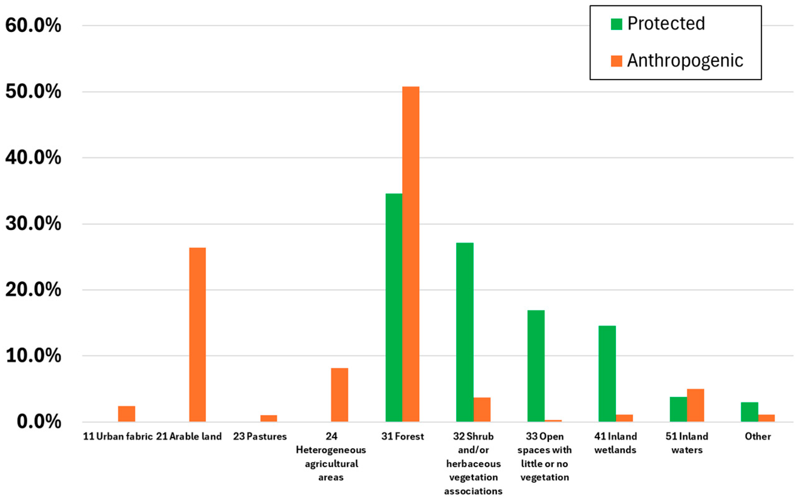
The CLC data were applied for two complementary purposes. First, they supported the binary classification task of distinguishing between wilderness and anthropogenic areas. The anthropogenic class was derived from high-impact CLC categories, specifically class 1 (artificial surfaces) and class 2 (agricultural areas). These regions represent areas of continuous human influence and were filtered to include only patches larger than 50 km2. Second, for the semantic segmentation task, the complete CLC nomenclature was employed to assign one of 44 thematic land-cover classes to each pixel, allowing for a more detailed interpretation of model predictions across diverse landscapes. The most prevalent CLC categories within the AnthroProtect dataset include urban fabric (11), arable land (21), pastures (23), forest (31), shrub and/or herbaceous vegetation associations (32), and inland wetlands (41). Analysis of class distribution revealed that arable land (21), urban fabric (11), and heterogeneous agricultural areas (24) occur exclusively within anthropogenic samples, whereas forest (31) is substantial in both wilderness (34.6%) and anthropogenic (50.8%) classes, highlighting its mixed representation across land-use types. On the other hand, wild areas are categorised as strict nature reserves (Ia), wilderness (Ib), and national parks (II).
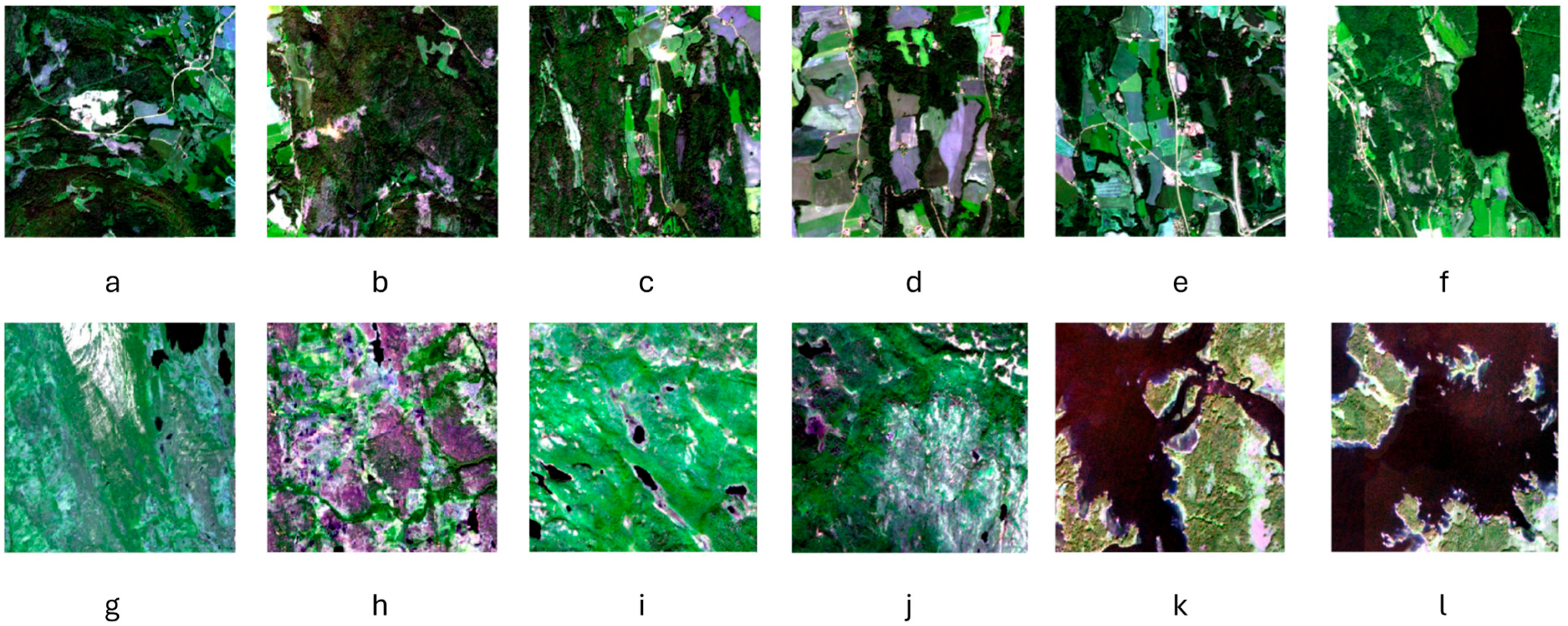
Figure 1 shows the spatial distribution of the labels (training, validation, and testing) and category types (wild, anthropogenic). Figure 2 shows the percentage of wild and anthropogenic categories vs. CLC classes in the study area. Figure 3 shows examples of image tiles for each category.
The AnthroProtect dataset was designed to train neural networks at the image level and was also exploited to evaluate different attribution methods at the pixel-wise level. To this purpose, Stomberg et al. divided the dataset into three subsets, 80% training, 10% validation, and 10% testing, ensuring their independence and spatial consistency [45]. Based on their results, the authors report that anthropogenic influences (e.g., villages) and agricultural areas can be well-mapped, and the deforestation areas can be well-detected. Moreover, different patterns occurring in forests can be distinguished. Conversely, the authors highlighted that models trained with AnthroProtect are likely not able to process applicable different ecosystems such as savannas or tropical forests [45].

2.3. Methods

This study considered two different tasks:
  • Image classification: A machine learning task that uses a model to map the input to a discrete output [47]. This task labels each image tile of the AnthroProtect dataset as ‘wild’ or ‘anthropogenic’.
  • Semantic segmentation: A deep learning task aiming to label every image pixel or image object/segment (i.e., a group of image pixels with similar features) into different land cover categories [48]. This task assigns each image pixel of the AnthroProtect dataset to one of the 44 thematic classes of the CORINE Land Cover (Figure 2).
The final is to provide some insights on optimising performance over accuracy by evaluating the impact of different
  • Batch sizes;
  • Architectures;
  • Spectral band setups.

2.3.1. Data Pre-Processing

Pre-processing involved the rescaling and normalisation of data.
We used Z-score normalisation to preserve the shape of the original data distribution and align it to a standard scale (mean of 0 and standard deviation of 1), thus making the data processing less sensitive to outliers [49]. Therefore, the input data were transformed according to Equations (1) and (2):
x s c = x s f ,
z = x s c μ B i σ B i ,
where x is the original pixel value, x s c is the scaled pixel value, s f is the scale factor, z is the normalised pixel value, μ B i is the mean pixel value for the spectral band i, and σ B i is the pixel standard deviation for spectral band i.
Regarding the scale factor ( s f ), out of the many approaches proposed in the literature, we opted for a mix of domain expertise-based and data-driven strategy. Starting from a range of values between 8 × 10 3 and 10 × 10 4 suggested by the domain experts, the scale factor was calculated by maximising the classification accuracy, with all other parameters fixed.

2.3.2. Image Classification Task

Architecture
Convolutional Neural Networks (CNNs), especially Residual Networks (ResNets), are efficient methods for classifying heterogeneous and complex scenes with high accuracy. ResNets’ key innovation is using residual connections in solving the vanishing gradient; the layers do not learn real mappings but residual functions to the layer input. Hence, this architecture can train very deep networks (more than 100 layers) without gradient flow issues.
Since satellite imagery presents unique challenges due to its high variability, complex spatial patterns, and massive data, the depth of ResNet models can help extract a rich set of features, from basic textures to complex land characteristics. Furthermore, despite their depth, ResNets are quite computationally efficient because each block in the model has shortcut connections that directly connect the block’s input with its output. This makes processing typical large satellite datasets feasible without requiring huge computation resources [50].
For all the reasons mentioned above and in the introduction, this study has focused on two ResNet models:
  • ResNet18: A network with 18 layers;
  • ResNet50: A network with 50 layers.
Batch Size
The choice of the batch size is a critical factor in deep learning and involves a trade-off between several factors, including computational resource allocation, learning stability, and training speed. The batch size directly affects the model’s performance [51], its ability to generalise on data [52], its computational efficiency and memory requirements [53], and how quickly [54] and stably [55] it learns.
  • Computational efficiency and memory requirements: Larger batch sizes simultaneously process a larger amount of data. This can lead to faster training because fewer iterations are needed to process the entire dataset. However, with the increase in batch sizes, memory use increases. On the other hand, smaller batch sizes require fewer memory resources, but more iterations are needed to process the whole dataset, and the training time increases significantly.
  • Convergence: Larger batch sizes might lead to faster training per epoch. However, they do not always result in more rapid convergence to a high-accuracy solution because of possible poor local minima. On the other hand, smaller batch sizes might lead to faster convergence because they can avoid poor local minima (though this might only sometimes prove to be true).
  • Stability, quality of learning, and generalisation capabilities: Larger batch sizes might lead to a more stable and reliable gradient estimate since the average takes over a larger amount of data, which can result in a smoother convergence. However, as stated before, it might also cause poorer performance in finding local minima, thus getting stuck in them and disrupting the generalisation. On the other hand, smaller batch sizes could introduce more noise in the training process. This can be beneficial because it provides a sort of regularisation and can lead to better generalisation on unseen data (i.e., validation and testing datasets); nevertheless, the noisiness might also make the process less stable.
For all the reasons mentioned above, this study has focused on the following batch sizes:
  • Medium batch size (64): This is a good trade-off between computational efficiency and the stochasticity of gradient updates.
  • Medium-large batch size (128): This is still a good trade-off between computational efficiency and the stochasticity of gradient updates and reduces the computation time.
  • Large batch size (256): This size leads to faster convergence but requires GPU processing, distributed computing (not always available), and careful tuning of hyperparameters.
Spectral Band Setup
The literature analysis pointed out that most machine-learning generic papers on agriculture and forestry use RGB input data [56,57], a combination of visible and NIR bands [58,59], or the full spectral setup [60], sometimes with the addition of vegetation indices [61,62,63]. While the abovementioned configurations are still the most widely used when focusing on deep learning papers [63,64,65], not all authors agree on the added value of vegetation indices [66].
For all the reasons mentioned above, this study has focused on the following spectral setups:
  • RGB: Sentinel-2 bands B2, B3, and B4.
  • RGB + NIR (RGBN): Sentinel-2 bands B2, B3, B4, and B8.
  • Full spectrum: Sentinel-2 bands B2, B3, B4, B5, B6, B7, B8, B8A, B11, and B12.
The RGB setup has the main advantage of being directly applicable for transfer learning with models pre-trained on natural images like ImageNet [57], making deployment more straightforward. On the other hand, RGBN and full spectrum setups make sense when studying wilderness because they provide more insight into vegetation status, stress, and biomass.

2.3.3. Semantic Segmentation Task

Architecture
Due to the complexity of satellite images, some models might offer a more robust design to capture more intricate patterns. This study has focused on the following models:
  • U-Net;
  • DeepLab V3;
  • FCN.
Specifically, U-Net is the lightest architecture (especially for standard configurations). It has become very useful for the semantic segmentation of remotely sensed images due to its innovative use of skip connections. These connections can bridge low-level detail with high-level semantic information across the encoder–decoder structure, thus enhancing localisation precision.
On the other hand, DeepLabV3 uses a ResNet50 backbone, which is heavier than U-Net but is particularly suitable for high-resolution satellite imagery, where the most important feature is detailed spatial information. Also, FCN uses a ResNet50 backbone, but its upsampling and prediction mechanisms are usually simpler than those in DeepLabV3. Thus, this architecture is lighter than DeepLabV3. FCN significantly contributed to advancing scene segmentation challenges, leveraging pre-defined convolutional kernels and their outputs, enhancing feature resolution, and enabling the prediction of each pixel’s class based on the highest probability value.
Batch Size
Semantic segmentation is much more computationally demanding than image classification. Consequently, in these experiments, we used only the following small batch sizes:
  • 2;
  • 4;
  • 8.
Spectral Band Setup
All the image classification task considerations also stand for the semantic segmentation task. Thus, we tested the same spectral setups described for image classification.

2.4. Software Implementation

A lightweight code was developed in Python (v3.10) [67] using the PyTorch framework (v2.0.1), Weights & Biases (v0.15) for experiment tracking and logging, NumPy (v1.24.4) and Pandas (v1.5.3) for math and data analytics, and TIFF (v2023.7.18) and scikit-learn (v1.2.2) for image processing and performance evaluation. To ensure reproducibility, the code sets a random seed for PyTorch, NumPy, and Python’s random modules, while for performance optimisation, it checks for GPU availability and sets the device accordingly.
As already described, the AnthroProtect dataset is designed with 80% of training data, 10% of validation data, and 10% of testing data. Using these ratios, we fed the training process with batches of shuffled data to guarantee randomisation [68]. Model training used the popular Adaptive Moment Estimation (Adam) [69] optimisation algorithm. Adam combines the best properties of the stochastic gradient descent extensions AdaGrad and RMSProp, which makes it a highly efficient algorithm even when gradients are sparse or fluctuating. Moreover, Adam is known for its computational efficiency and low memory footprint. Cross Entropy (CE) was used as the loss function because it is tailored for image classification and segmentation and for its smooth gradient flow that avoids vanishing or exploding gradients. Model performance was evaluated with unshuffled validation data to ensure reproducibility, and the model accuracy was assessed using the unseen testing dataset.
In our image classification experiments, we impact the efficiency of pre-trained models. Specifically, we employed the ResNet18 and ResNet50 models, both pre-trained on the ImageNet dataset. To adapt these models to our needs, we modified the initial convolutional layer to accommodate input images with variable spectral bands. Additionally, we adjusted the fully connected layers to output two classes (i.e., wild and anthropogenic).
For the semantic segmentation experiments, transfer learning was used with PyTorch implementations of DeepLabV3 and FCN, which employ a ResNet50 backbone pre-trained on ImageNet. Due to the absence of U-Net in the PyTorch library, we coded a custom implementation based on its original paper [31]; therefore, we did not use transfer learning for U-Net. Performance metrics for semantic segmentation also include the mIoU calculated on the testing dataset.

2.5. Computation Constraints and Experimental Setup

Regarding the experimental setup, the optimal scale factor was estimated as 1 × 10 4 and set in all the experiments. In addition, all the experiments used a learning rate of 1 × 10 3 and a weight decay factor of 1 × 10 4 .
Image classification was trained with 50 epochs. It should be mentioned that, for the ResNet50 architecture, computational power allowed only the use of the medium batch size (64).
On the other hand, due to limited computational resources and long processing time, semantic segmentation was trained with 20 epochs.

3. Results

3.1. Image Classification Task

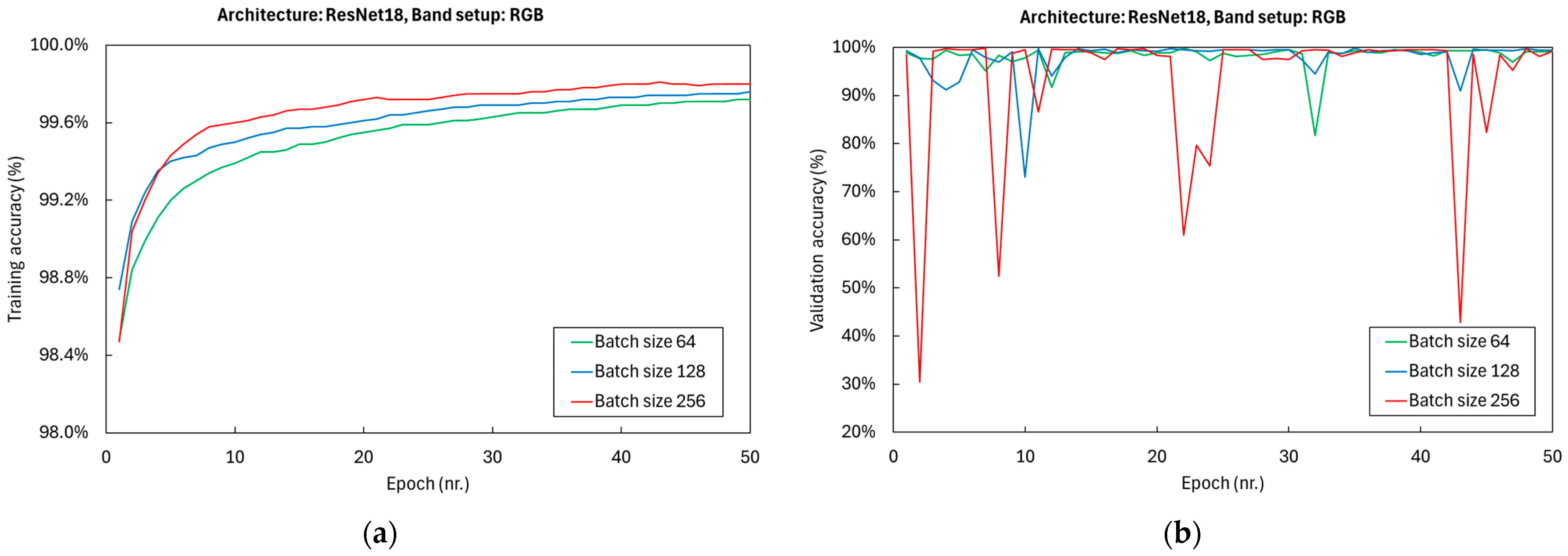
Figure 4 shows the impact of the batch size. These experiments used the RGB band setup to represent most transfer-learning applications. Moreover, as discussed in the Section ‘Materials and Methods’, these experiments were not performed with the ResNet50 architecture due to its excessive computational requests.
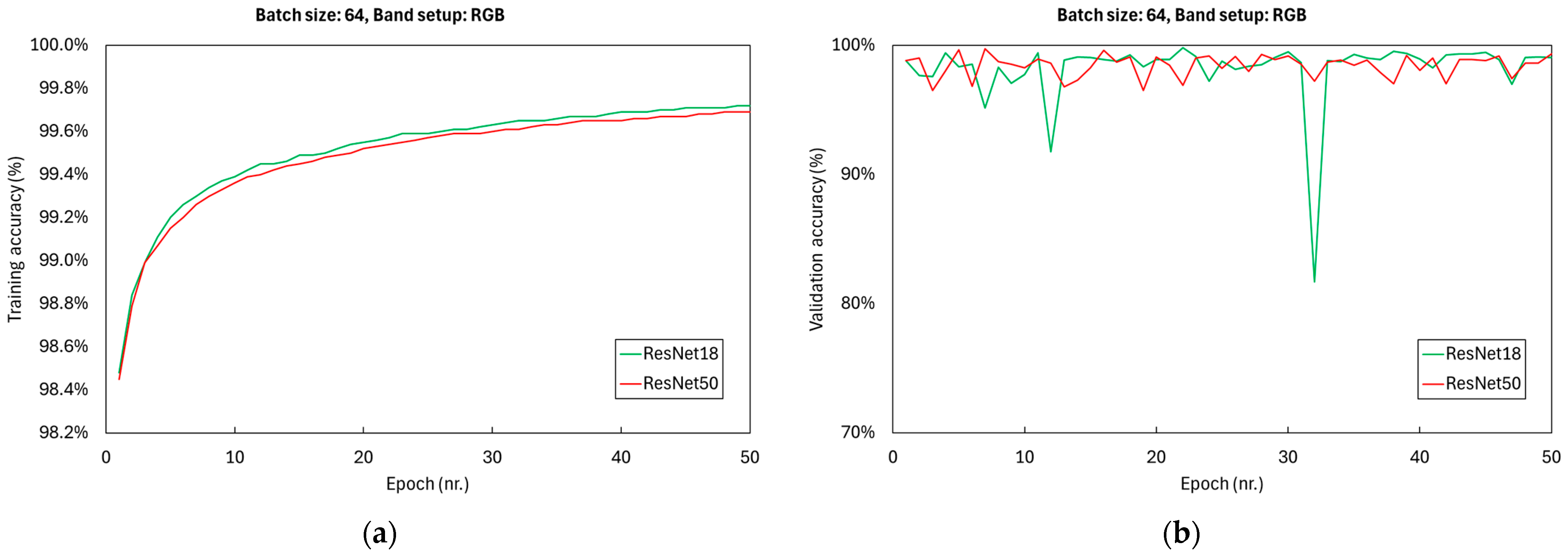
Figure 5 shows the impact of the architecture. These experiments used the RGB band setup for the reason mentioned above and the medium batch size because it has a smaller footprint on memory, which is often a concern when training on limited computational resources.
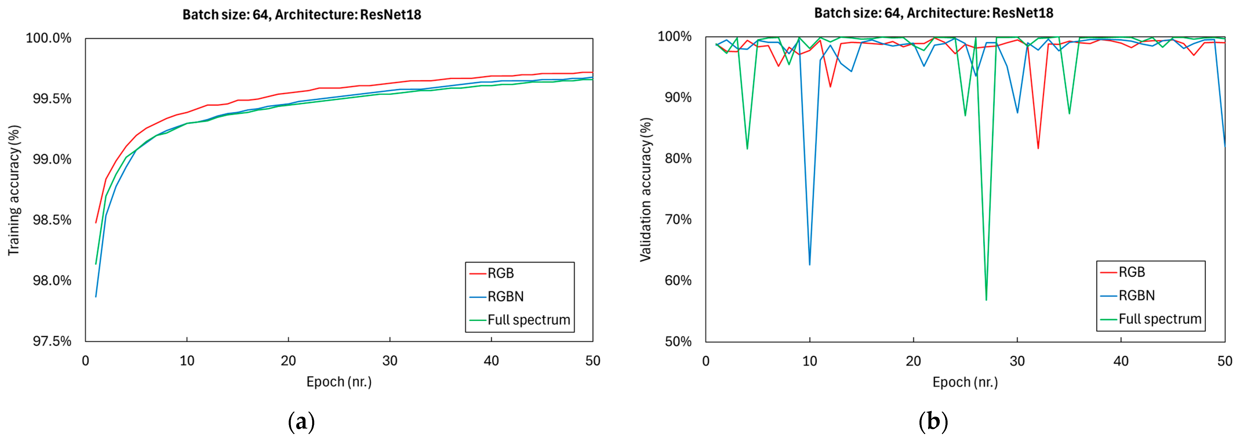
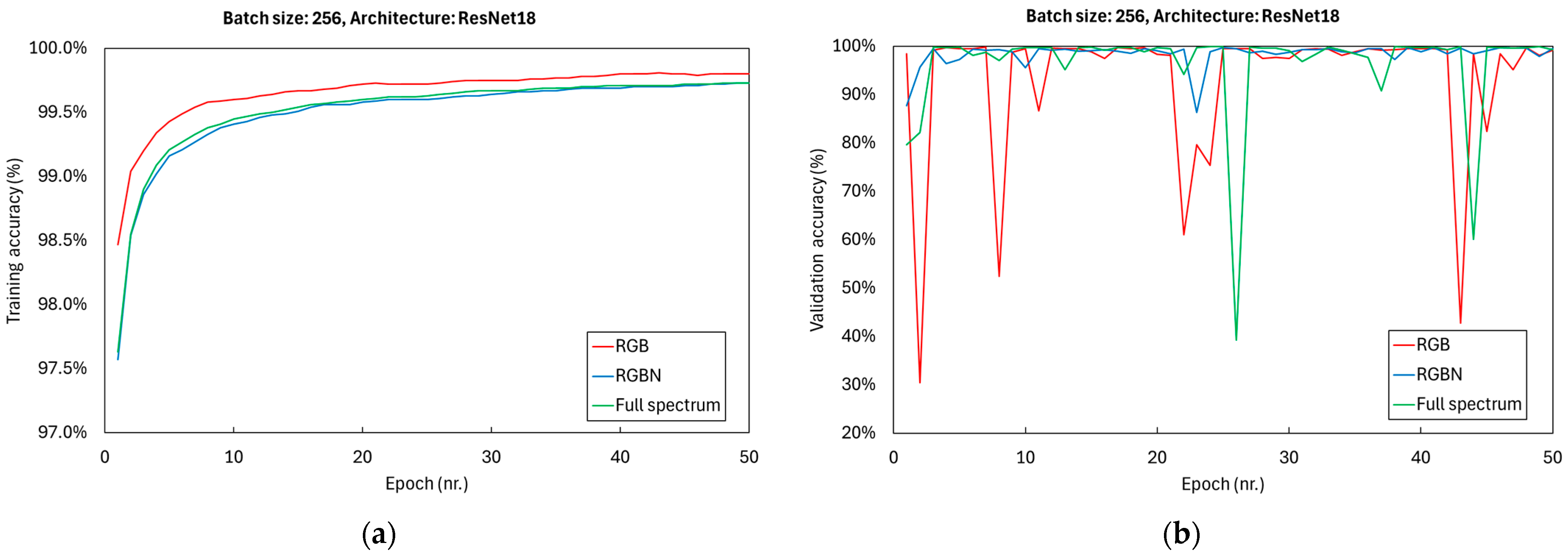
Figure 6 and Figure 7 show the impact of the band setup with medium and large batch sizes. Again, these experiments were not performed with the ResNet50 architecture due to its excessive computational requests.
Table 1 shows the calculation times and accuracies for different configurations.
In addition to overall accuracy, the F1 score was also computed to ensure a more balanced evaluation of the classification performance. The F1 score, which represents the harmonic mean of precision and recall, provides a less misleading measure than high accuracy alone, especially when class distributions are unbalanced. In this case, the F1 score reached values consistent with the testing accuracy, confirming that the models maintained a balanced sensitivity and precision across both the wild and the anthropogenic classes.

3.2. Semantic Segmentation

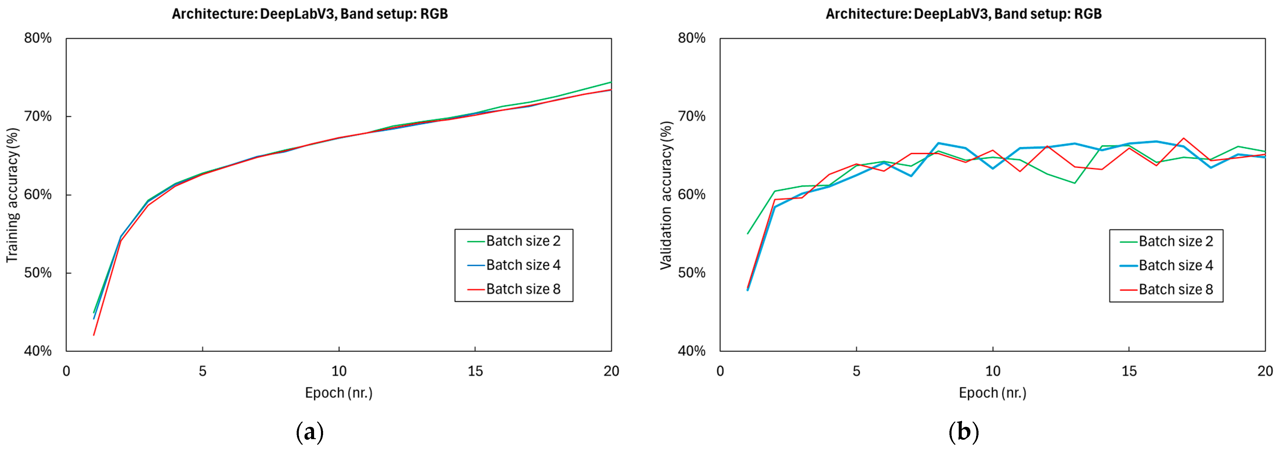
Figure 8 shows the impact of the batch size. These experiments used the RGB band setup to represent most transfer-learning applications.
Figure 9 shows the impact of the architecture. These experiments used the RGB band setup for the reason mentioned above and batch size 4 as a compromise between computation resources and accuracy.
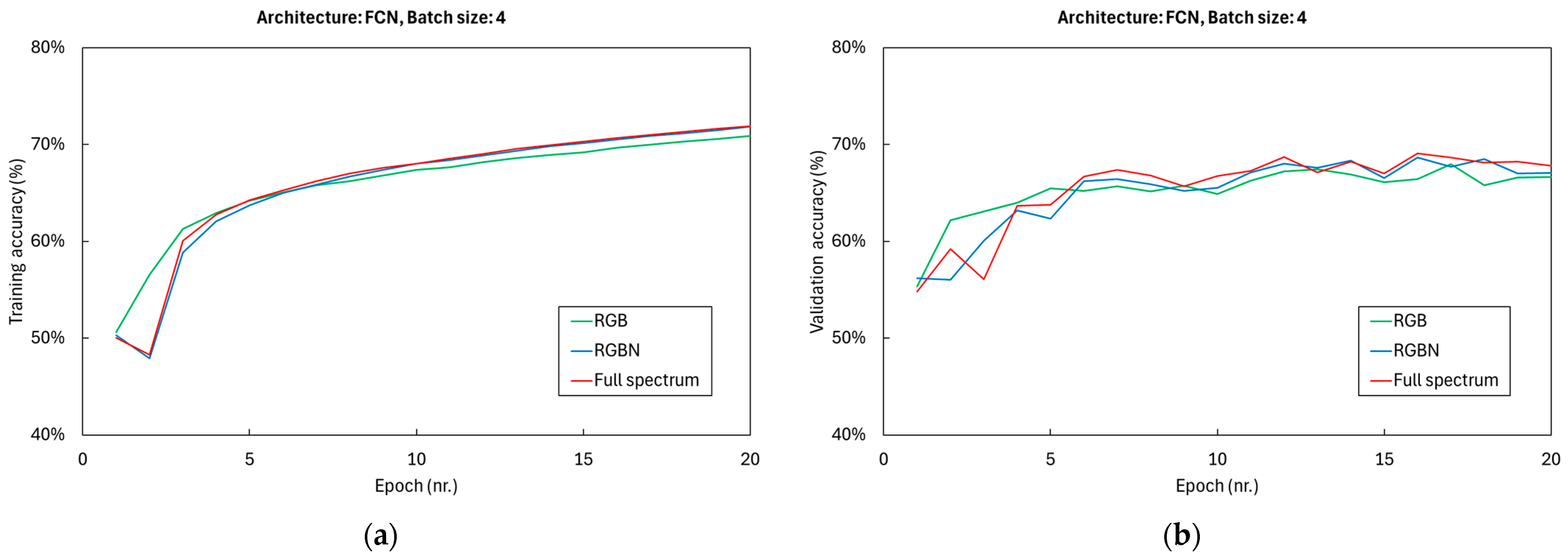
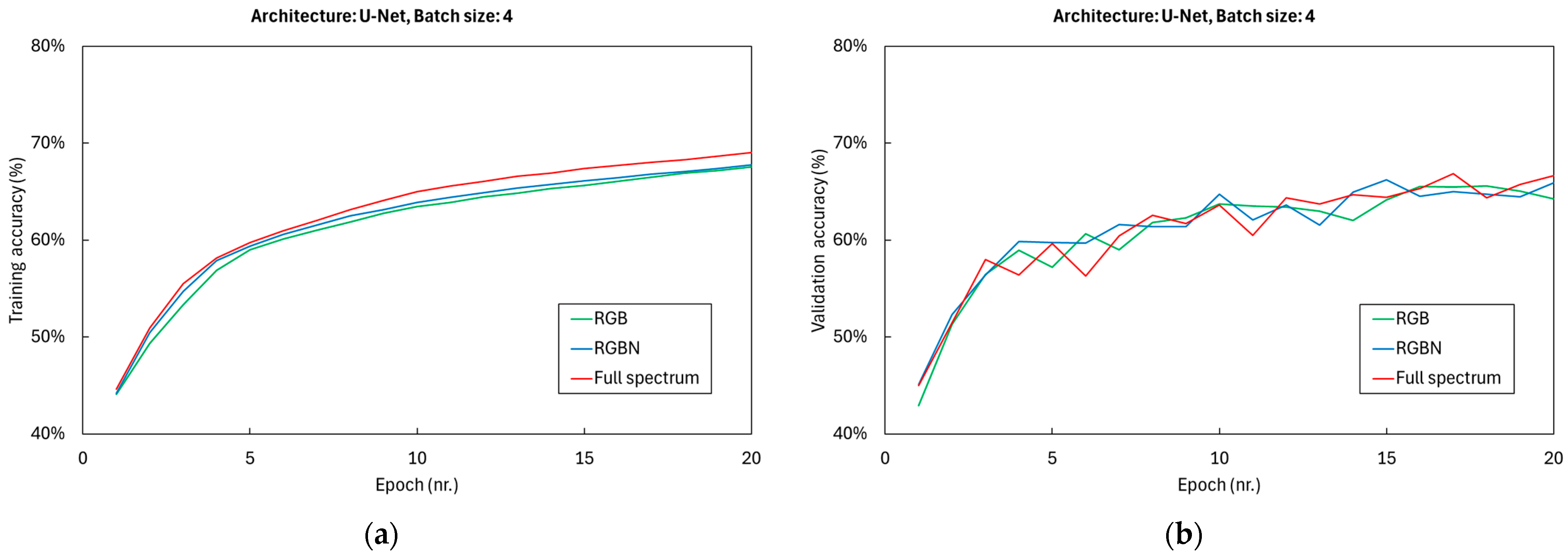
Figure 10, Figure 11 and Figure 12 show the impact of the band setup for all the architectures considered.
Table 2 shows the calculation times and accuracies for different configurations.

4. Discussion

4.1. Image Classification Task

4.1.1. Impact of Batch Size

Figure 4 and Table 1 show that the batch size does not significantly impact the accuracy of our experiments; the final accuracies (training: 99.72–99.80%; validation: 99.04–99.16%; testing: 99.54–99.67%) are almost identical, thus suggesting that any difference can be interpreted as the randomness of outcomes. On the other hand, batch size has a big impact on the calculation time. For instance, the largest batch size (256) reduced the calculation time by 69% compared to the medium batch size (64), highlighting the potential efficiency that can be achieved.
At the same time, as batch size increases, the training learning curve becomes steeper (Figure 4a). Still, when the model’s performance is evaluated on the validation dataset, the validation learning curve shows random declining spikes (Figure 4b). This effect also occurs using medium (64) and medium-large (128) batch sizes, but to a lesser extent, with an overall increase in reliability and stability of the model’s training.
Our experiments show that the largest batch size (256) is optimal, subject to suitable computing resources and assuming sufficient training epochs to guarantee convergence. A sub-optimal solution could be the medium-large (128) batch size, at the expense of calculation efficiency (+75% compared to the largest batch size, still −46% compared to the medium batch size) but leading to a more stable validation learning curve, which is not so dependent on the training epochs.

4.1.2. Impact of Architecture

Regarding the impact of the architecture, Figure 5 and Table 2 show that it does not significantly impact the accuracy of our experiments. The final accuracies (training: 99.66–99.72%; validation: 99.04–99.71%; testing: 99.54–99.79%) are almost identical, thus suggesting, also in this case, that any difference can be interpreted as the randomness of outcomes. On the other hand, architecture affects calculation time, and the more complex ResNet50 network required +57% calculation time than the simpler ResNet18, with no apparent benefits on the training learning curve (Figure 5a) but with a smoothing effect on the random declining spikes seen on the validation learning curve (Figure 5b).
Our experiments show that ResNet18 is the optimal architecture. It provides computational benefits regarding calculation time and memory usage without significantly reducing the accuracy.

4.1.3. Impact of Spectral Band Setup

Figure 6 and Figure 7 and Table 1 show the impact of spectral band setup. As discussed later, these experiments were performed only for ResNet18 due to computational constraints.
Our experiments showed that the band setup does not influence the final accuracy. Whether using the optimal large batch size (256) or the inefficient medium batch size (64), all scenarios led to testing accuracies higher than 99.4%. However, given the almost perfect classification accuracy, that seems a reasonable result and not a shortcoming. Moreover, the training learning curves are very close to each other (Figure 6a and Figure 7a), but the validation learning curves show similar random declining spikes as observed when testing different batch sizes. However, spikes cannot be related to a specific band setup (Figure 6b and Figure 7b).

4.2. Semantic Segmentation Task

4.2.1. Impact of Batch Size

Figure 8 and Table 2 show that batch size has a minimal impact on the accuracy of our experiments. The final accuracies (training: 73.40–74.39%; validation: 65.54–67.11%; testing: 66.80–67.11%) have close values, with a slight preference for batch size 4. In addition, the training learning curves are perfectly overlapping (Figure 8a), and the validation learning curves show a similar degree of fluctuation (Figure 8b). From a calculation point of view, the tiny differences observed (0.3–0.5%) are also insignificant.
Our experiments did not identify a clear optimal batch size. Given the negligible differences in calculation time, there is a slight preference for batch size 4 when looking at validation and testing accuracies and a slight preference for batch size 8 when looking at the mIoU. Thus, both setups are sub-optimal, but in the light of optimising computation resources vs. accuracy, batch size 4 might be preferred.

4.2.2. Impact of Architecture

Regarding the impact of the architecture, Figure 9 and Table 2 show contradictory outcomes. When evaluating the training accuracy, DeepLabV3 (74.39%) overperforms FCN (70.90%) and U-Net (67.57%). Also, the training learning curves (Figure 9a) and the testing learning curves (Figure 9b) display an overperformance of DeepLabV3 and FCN over U-Net. However, when evaluating validation and testing accuracies and mIoU, all the architectures are close together, with less than a 2.4% spread. What is not negligible is the calculation time: U-Net is the fastest, FCN requires +20% time, and DeepLabV3 requires +62% time.
Our experiments show that FCN is the optimal architecture when considering only the model’s accuracy. However, U-Net is an attractive sub-optimal solution when searching for a trade-off between computation resources vs. accuracy.

4.2.3. Impact of Spectral Band Setup

The impact of the spectral band setup is shown in Figure 10, Figure 11 and Figure 12 and Table 2. For all the architectures tested, the main hint of our experiments is that band setup has a minimal impact on accuracy. The final accuracies (training: 72.60–74.39%; validation: 64.80–66.82%; testing: 66.80–67.72%) have close values, without a clear winner. Also, the values of mIoU are very close (within a spread of 0.19%). In addition, the training learning curves (Figure 9a, Figure 10a and Figure 11a) and the validation learning curves (Figure 10b, Figure 11b and Figure 12b) are rather similar.
Our experiments also showed that increasing the number of spectral bands did not correlate with increased computing time, which is valid for all the architectures tested (Table 2). The fastest processing always uses three bands (RGB), and adding more bands increases the calculation time from 2% for DeepLabV3 to approximately 10% for FCN. And it only sometimes takes longer to process the full spectral setup than RGBN.
This outcome raises critical thinking on the networks’ real ability to fully exploit the spectral information of the input data and the effectiveness of transfer learning in Geosciences when using pre-trained networks with generic or web-based data, such as ImageNet. If it was plausible to expect this result from pre-trained networks on non-EO specific three-band images (i.e., DeepLabV3 and FCN), the result with U-Net seems to confirm that this is not a peculiar characteristic of pre-trained networks, and more investigation is needed.

4.3. Comparison with Similar Studies

As mentioned, we found a few similar studies in the literature, sometimes with a different focus and often using different models/techniques. Thus, a straightforward comparison of results is not possible. Nevertheless, despite this limitation, our outcomes align well with the existing literature. For instance, Wagner et al. (2019) [70] proposed a U-Net architecture for mapping different forest types and detecting disturbances in the Brazilian Atlantic rainforest with high-resolution optical images. The authors described an accuracy of about 95% using RGB images, limited training epochs (between 25 and 28), and small batch sizes (between 8 and 16). Moreover, their study concluded that there might be better methods than the U-Net architecture for this purpose, but its high performance and relative ease of use make up for it. Those results are comparable to our outcomes.
Hizal et al. (2024) [71] tested two different band configurations (RGB and RGBN) in a forestry setting in Turkey. Similarly to our study, the authors used DeepLab (and PSPNet), which were pre-trained on ImageNet. They also used batch sizes similar to ours and reported accuracies in semantic segmentation comparable to ours (most classes with mIoU above 70%).
Other studies, such as Waldeland et al. (2022) [72], Brandt et al. (2020) [73], and de Bem et al. (2020) [74], despite having different objectives, achieved comparable results to our experiments in similar regions and using similar deep learning architectures (U-Net and FCN). That by Sylvain et al. (2019) [75] stands out. This research analysed the Quebec forestry with the following similarities with our work:
  • The vegetation was similar, with many species of birch, aspen, and needle leaf in both biomes [76];
  • The presence of different degrees of forestry management activities;
  • The use of RGB and RGBN optical images;
  • The use of ResNet architecture with batches made of 256 images.
In a four-class image classification, the authors reported testing and validation accuracies above 93%, which is just slightly below our results (but we used only two classes). Moreover, the authors reported an overall accuracy above 90% in nine-class image classification, suggesting that alternative CNN-based approaches, like FCN, should have been tested.
Overall, the existing literature demonstrates the effectiveness of deep learning for remote sensing in forestry and related fields. Our results are consistent with previous studies and offer new insights into wilderness.

4.4. Current Limitations and Future Perspectives

The results of this study provide some first insights into the optimisation of deep neural networks for wilderness. However, results were constrained by the following limitations:
  • Computational resources: More computational power was required to run all the experiments with the demanding ResNet50 architecture. Moreover, slow processing limited semantic segmentation experiments due to limited computational resources. Overall, with more resources and faster data processing, we could have tested more combinations of parameters. However, our focus was on limited computational resources.
  • Dataset: This study focused only on the AnthroProtect dataset, which was built ad hoc to study wilderness. Unfortunately, we could not test the architectures on other data. This limitation is also due to the enormous effort required to build such a dataset.
These limitations have led to some cut-offs when considering what to include in the study and what to leave out. Thus, given the current results, future work should investigate more in depth some of the following aspects:
  • The contribution of larger batch sizes.
  • The contribution of each spectral band, with a specific focus on the individual contribution to accuracy. Also, the architectures used in this study have been optimised to work on RGB images. It would be interesting to investigate what this means in terms of using a multiclass and multispectral dataset and if any change could be implemented to the architectures fully to exploit the spectral richness of input data.
  • Linked to the previous point, the impact of hyperspectral data on wilderness studies.
  • The investigation of more recent and less commonly used neural networks, such as EfficientNets or VisionTransformers (ViTs), which might offer improvements in both image classification and semantic segmentation. However, our focus was on already well-known and used architectures.
  • A deeper investigation of the trade-off between training efficiency and final accuracy. In this regard, it would make sense to explore techniques such as adaptive batch sizing or optimisation algorithms that can dynamically adjust during training.
  • Finally, testing deep learning on different wilderness datasets. Ongoing research on foundational models increasingly focuses on their applications in satellite imaging, which is an interesting direction that warrants further investigation.

5. Conclusions

This work has explored the optimisation of deep learning architectures for image classification and semantic segmentation of wilderness areas and their naturalness using satellite remote sensing imagery. Based on the available literature, only a few studies have addressed this subject so far.
While high-dimensional datasets are very informative, their complexity might hide the keys to some insights, and the architecture of deep learning models is a critical factor in determining their effectiveness. The more simplistic models risk missing subtleties, while the overly complex ones are often impracticable in real-life applications due to excessive computational loads and overfitting. Given limited computation resources (not always considered in this kind of study), optimality was sought in the compromise between model and data complexity and dimensionality. Specifically, we have focused on three dimensions: batch size, model architecture, and spectral band setup.
Regarding the image classification task, the final accuracy generally scored above 98%. Thus, choosing an optimal configuration had to originate from considerations of memory use, computation time, and overall efficiency rather than significant differences in classification accuracy. Out of all the experiments, the optimal setup was found in the ResNet18 architecture, using input images passed in size 256 or 64 batches.
Concerning the evaluation of semantic segmentation task, this task was tricky because the architectures tested were not immediately comparable, unlike image classification. Moreover, the experiments did not identify a clear optimal batch size. Nevertheless, the U-Net architecture emerged as an attractive sub-optimal solution.
The use of different numbers of input spectral bands deserves a separate comment. Our experiments highlighted no significant impact on the computation time or final accuracy both for image classification and semantic segmentation. This outcome raises critical thinking on the usefulness of transfer learning in EO and Geosciences in general, when the networks are pre-trained with a generic dataset (such as ImageNet) that is not specific to the application field.
Finally, it is important to note that this study relied on the AnthroProtect dataset, which is made of Sentinel-2 image tiles. Consequently, in any operational setting using optical data, pre-processing steps—such as atmospheric correction, geometric correction, and cloud masking—are essential and can introduce potential sources of bias in the final outputs. Furthermore, the spatial resolution of Sentinel-2 (10–20 m) poses challenges when analysing heterogeneous landscapes or small-scale features, as widely documented in the literature, potentially leading to biases in land cover classification products.

Author Contributions

Methodology, G.V.; software, G.V.; validation, G.V. and M.G.; formal analysis, G.V. and M.G.; investigation, G.V.; data curation, G.V.; writing—original draft preparation, G.V., M.G. and N.G.; writing—review and editing, G.V., M.G. and N.G.; supervision, M.G. All authors have read and agreed to the published version of the manuscript.

Funding

Research funded by the Erasmus+ Programme.

Data Availability Statement

The original data presented in the study are openly available. The AnthroProtect dataset is available on the University of Bonn—Remote Sensing Group website at https://rs.ipb.uni-bonn.de/data/anthroprotect/ (accessed on 20 September 2025). The source code for the optimisation of deep learning parameters for classification and segmentation of wilderness areas with Copernicus Sentinel-2 images is available in Zenodo at https://doi.org/10.5281/zenodo.12721167 (accessed on 20 September 2025).

Acknowledgments

The authors are grateful to Ribana Roscher (University of Bonn), Ahmed Emam (University of Bonn), and Mohamed Ibrahim (University of Bonn) for the design of the experimental setup, software implementation, and access to the computing resources at the of University of Bonn.

Conflicts of Interest

The authors declare no conflicts of interest.

References

  1. Di Marco, M.; Ferrier, S.; Harwood, T.D.; Hoskins, A.J.; Watson, J.E.M. Wilderness areas halve the extinction risk of terrestrial biodiversity. Nature 2019, 573, 582–585. [Google Scholar] [CrossRef]
  2. Watson, J.E.M.; Evans, T.; Venter, O.; Williams, B.; Tulloch, A.; Stewart, C.; Thompson, I.; Ray, J.C.; Murray, K.; Salazar, A.; et al. The exceptional value of intact forest ecosystems. Nat. Ecol. Evol. 2018, 2, 599–610. [Google Scholar] [CrossRef]
  3. Maxwell, S.L.; Cazalis, V.; Dudley, N.; Hoffmann, M.; Rodrigues, A.S.L.; Stolton, S.; Visconti, P.; Woodley, S.; Kingston, N.; Lewis, E.; et al. Area-based conservation in the twenty-first century. Nature 2020, 586, 217–227. [Google Scholar] [CrossRef] [PubMed]
  4. Allan, J.R.; Venter, O.; Watson, J.E.M. Temporally inter-comparable maps of terrestrial wilderness and the Last of the Wild. Sci. Data 2017, 4, 170187. [Google Scholar] [CrossRef]
  5. Ekim, B.; Stomberg, T.T.; Roscher, R.; Schmitt, M. MapInWild: A remote sensing dataset to address the question of what makes nature wild [Software and Data Sets]. IEEE Geosci. Remote Sens. Mag. 2023, 11, 103–114. [Google Scholar] [CrossRef]
  6. Emam, A.; Farag, M.; Roscher, R. Confident Naturalness Explanation (CNE): A Framework to Explain and Assess Patterns Forming Naturalness Motivation. IEEE Geosci. Remote Sens. Lett. 2024, 21, 8500505. [Google Scholar] [CrossRef]
  7. Emam, A.; Stomberg, T.; Roscher, R. Leveraging Activation Maximization and Generative Adversarial Training to Recognize and Explain Patterns in Natural Areas in Satellite Imagery Motivation. IEEE Geosci. Remote Sens. Lett. 2024, 21, 8500105. [Google Scholar] [CrossRef]
  8. Raiyani, K.; Gonçalves, T.; Rato, L.; Salgueiro, P.; Marques da Silva, J.R. Sentinel-2 Image Scene Classification: A Comparison between Sen2Cor and a Machine Learning Approach. Remote Sens. 2021, 13, 300. [Google Scholar] [CrossRef]
  9. Cheng, G.; Xie, X.; Han, J.; Guo, L.; Xia, G.-S. Remote Sensing Image Scene Classification Meets Deep Learning: Challenges, Methods, Benchmarks, and Opportunities. IEEE J. Sel. Top. Appl. Earth Obs. Remote Sens. 2020, 13, 3735–3756. [Google Scholar] [CrossRef]
  10. Saha, S.; Shahzad, M.; Mou, L.; Song, Q.; Zhu, X.X. Unsupervised Single-Scene Semantic Segmentation for Earth Observation. IEEE Trans. Geosci. Remote Sens. 2022, 60, 5228011. [Google Scholar] [CrossRef]
  11. Khan, S.D.; Basalamah, S. Multi-Branch Deep Learning Framework for Land Scene Classification in Satellite Imagery. Remote Sens. 2023, 15, 3408. [Google Scholar] [CrossRef]
  12. Ouma, Y.O.; Keitsile, A.; Nkwae, B.; Odirile, P.; Moalafhi, D.; Qi, J. Urban land-use classification using machine learning classifiers: Comparative evaluation and post-classification multi-feature fusion approach. Eur. J. Remote Sens. 2023, 56, 2173659. [Google Scholar] [CrossRef]
  13. Vali, A.; Comai, S.; Matteucci, M. Deep Learning for Land Use and Land Cover Classification Based on Hyperspectral and Multispectral Earth Observation Data: A Review. Remote Sens. 2020, 12, 2495. [Google Scholar] [CrossRef]
  14. Dimitrovski, I.; Kitanovski, I.; Kocev, D.; Simidjievski, N. Current Trends in Deep Learning for Earth Observation: An Open-Source Benchmark Arena for Image Classification. ISPRS J. Photogramm. Remote Sens. 2023, 197, 18–35. [Google Scholar] [CrossRef]
  15. Hoeser, T.; Kuenzer, C. Object Detection and Image Segmentation with Deep Learning on Earth Observation Data: A Review-Part I: Evolution and Recent Trends. Remote Sens. 2020, 12, 1667. [Google Scholar] [CrossRef]
  16. Yu, X.; Li, S.; Zhang, Y. Incorporating convolutional and transformer architectures to enhance semantic segmentation of fine-resolution urban images. Eur. J. Remote Sens. 2024, 57, 2361768. [Google Scholar] [CrossRef]
  17. El Sakka, M.; Mothe, J.; Ivanovici, M. Images and CNN applications in smart agriculture. Eur. J. Remote Sens. 2024, 57, 2352386. [Google Scholar] [CrossRef]
  18. LeCun, Y.; Bengio, Y.; Hinton, G. Deep learning. Nature 2015, 521, 436–444. [Google Scholar] [CrossRef]
  19. Rumelhart, D.E.; Hinton, G.E.; Williams, R.J. Learning representations by back-propagating errors. Nature 1986, 323, 533–536. [Google Scholar] [CrossRef]
  20. Liang, J.; Xu, J.; Shen, H.; Fang, L. Land-use classification via constrained extreme learning classifier based on cascaded deep convolutional neural networks. Eur. J. Remote Sens. 2020, 53, 219–232. [Google Scholar] [CrossRef]
  21. Krizhevsky, A.; Sutskever, I.; Hinton, G.E. ImageNet Classification with Deep Convolutional Neural Networks. In Proceedings of the 26th Annual Conference on Neural Information Processing Systems, Lake Tahoe, NV, USA, 3–6 December 2012; ISBN 9781627480031. Available online: https://proceedings.neurips.cc/paper/2012 (accessed on 20 September 2025).
  22. Coţolan, L.; Moldovan, D. Applicability of pre-trained CNNs in temperate deforestation detection. Eur. J. Remote Sens. 2024, 57, 2367221. [Google Scholar] [CrossRef]
  23. Simonyan, K.; Zisserman, A. Very deep convolutional networks for large-scale image recognition. In Proceedings of the 3rd International Conference on Learning Representations, San Diego, CA, USA, 7–9 May 2015; pp. 1–14. Available online: https://dblp.org/db/conf/iclr/iclr2015.html (accessed on 20 September 2025).
  24. Gao, Y.; Shi, J.; Li, J.; Wang, R. Remote sensing scene classification based on high-order graph convolutional network. Eur. J. Remote Sens. 2021, 54 (Suppl. S1), 141–155. [Google Scholar] [CrossRef]
  25. Szegedy, C.; Liu, W.; Jia, Y.; Sermanet, P.; Reed, S.; Anguelov, D.; Erhan, D.; Vanhoucke, V.; Rabinovich, A. Going deeper with convolutions. In Proceedings of the 2015 IEEE Conference on Computer Vision and Pattern Recognition, Boston, MA, USA, 7–12 June 2015; pp. 1–9. [Google Scholar] [CrossRef]
  26. He, K.; Zhang, X.; Ren, S.; Sun, J. Deep Residual Learning for Image Recognition. In Proceedings of the 2016 IEEE Conference on Computer Vision and Pattern Recognition, Las Vegas, NV, USA, 27–30 June 2016; pp. 770–778. [Google Scholar] [CrossRef]
  27. Huang, G.; Liu, Z.; van der Maaten, L.; Weinberger, K.Q. Densely Connected Convolutional Networks. In Proceedings of the 2017 IEEE Conference on Computer Vision and Pattern Recognition, Honolulu, HI, USA, 21–26 July 2017. [Google Scholar] [CrossRef]
  28. Tan, M.; Le, Q.V. EfficientNet: Rethinking Model Scaling for Convolutional Neural Networks. In Proceedings of the 36th International Conference on Machine Learning, Long Beach, CA, USA, 10–15 June 2019; Available online: https://proceedings.mlr.press/v97/ (accessed on 20 September 2025).
  29. Long, J.; Shelhamer, E.; Darrell, T. Fully Convolutional Networks for Semantic Segmentation. In Proceedings of the 2015 IEEE Conference on Computer Vision and Pattern Recognition, Boston, MA, USA, 7–12 June 2015; pp. 3431–3440. [Google Scholar] [CrossRef]
  30. Badrinarayanan, V.; Kendall, A.; Cipolla, R. Segnet: A deep convolutional encoder-decoder architecture for image segmentation. IEEE Trans. Pattern Anal. Mach. Intell. 2017, 39, 2481–2495. [Google Scholar] [CrossRef]
  31. Ronneberger, O.; Fischer, P.; Brox, T. U-Net: Convolutional Networks for Biomedical Image Segmentation. In Proceedings of the International Conference on Medical Image Computing and Computer-Assisted Intervention, Munich, Germany, 5–9 October 2015; Volume 9351, pp. 234–241. [Google Scholar] [CrossRef]
  32. Chen, L.-C.; Papandreou, G.; Kokkinos, I.; Murphy, K.; Yuille, A.L. Deeplab: Semantic image segmentation with deep convolutional nets, atrous convolution, and fully connected crfs. IEEE Trans. Pattern Anal. Mach. Intell. 2017, 40, 834–848. [Google Scholar] [CrossRef]
  33. Chen, L.-C.; Zhu, Y.; Papandreou, G.; Schroff, F.; Adam, H. Encoder-decoder with atrous separable convolution for semantic image segmentation. In Proceedings of the European conference on computer vision (ECCV), Munich, Germany, 8–14 September 2018; pp. 801–818. [Google Scholar]
  34. Skidmore, A.K.; Pettorelli, N.; Coops, N.C.; Geller, G.N.; Hansen, M.; Lucas, R.; Mücher, C.A.; O’Connor, B.; Paganini, M.; Pereira, H.M.; et al. Environmental Science: Agree on Biodiversity Metrics to Track from Space. Nature 2015, 523, 403–405. [Google Scholar] [CrossRef]
  35. Luque, S.; Pettorelli, N.; Vihervaara, P.; Wegmann, M. Improving Biodiversity Monitoring Using Satellite Remote Sensing to Provide Solutions Towards the 2020 Conservation Targets. Methods Ecol. Evol. 2018, 9, 1784–1786. [Google Scholar] [CrossRef]
  36. Giuliani, G.; Egger, E.; Italiano, J.; Poussin, C.; Richard, J.-P.; Chatenoux, B. Essential Variables for Environmental Monitoring: What Are the Possible Contributions of Earth Observation Data Cubes? Data 2020, 5, 100. [Google Scholar] [CrossRef]
  37. Ustin, S.L.; Middleton, E.M. Current and near-term advances in Earth observation for ecological applications. Ecol. Process. 2021, 10, 1. [Google Scholar] [CrossRef] [PubMed]
  38. Šandera, J.; Štych, P. Mapping changes of grassland to arable land using automatic machine learning of stacked ensembles and H2O library. Eur. J. Remote Sens. 2023, 57, 2294127. [Google Scholar] [CrossRef]
  39. Li, W.; Zuo, X.; Liu, Z.; Nie, L.; Li, H.; Wang, J.; Cui, L. Predictions of Spartina alterniflora leaf functional traits based on hyperspectral data and machine learning models. Eur. J. Remote Sens. 2023, 57, 2294951. [Google Scholar] [CrossRef]
  40. Morais, T.G.; Rodrigues, N.R.; Gama, I.; Domingos, T.; Teixeira, R.F.M. Development of an algorithm for identification of sown biodiverse pastures in Portugal. Eur. J. Remote Sens. 2023, 56, 2238878. [Google Scholar] [CrossRef]
  41. Dang, K.B.; Nguyen, M.H.; Nguyen, D.A.; Phan, T.T.H.; Giang, T.L.; Pham, H.H.; Nguyen, T.N.; Tran, T.T.V.; Bui, D.T. Coastal Wetland Classification with Deep U-Net Convolutional Networks and Sentinel-2 Imagery: A Case Study at the Tien Yen Estuary of Vietnam. Remote Sens. 2020, 12, 3270. [Google Scholar] [CrossRef]
  42. Fisher, M.; The Wildland Research Institute. Review of Status and Conservation of Wild Land in Europe. 2010. Available online: http://www.self-willed-land.org.uk/rep_res/0109251.pdf (accessed on 20 September 2025).
  43. Sanderson, E.W.; Jaiteh, M.; Levy, M.A.; Redford, K.H.; Wannebo, A.V.; Woolmer, G. The Human Footprint and the Last of the Wild: The Human Footprint is a Global Map of Human Influence on the Land Surface, Which Suggests That Human Beings are Stewards of Nature, Whether We Like It or Not. BioScience 2002, 52, 891–904. [Google Scholar] [CrossRef]
  44. University of Bonn, Remote Sensing Group. AnthroProtect Dataset. Available online: https://rs.ipb.uni-bonn.de/data/anthroprotect/ (accessed on 20 September 2025).
  45. Stomberg, T.T.; Leonhardt, J.; Weber, I.; Roscher, R. Recognizing protected and anthropogenic patterns in landscapes using interpretable machine learning and satellite imagery. Front. Artif. Intell. 2023, 6, 1278118. [Google Scholar] [CrossRef] [PubMed]
  46. Gorelick, N.; Hancher, M.; Dixon, M.; Ilyushchenko, S.; Thau, D.; Moore, R. Google earth engine: Planetary-scale geospatial analysis for everyone. Remote Sens. Environ. 2017, 202, 18–27. [Google Scholar] [CrossRef]
  47. Zeng, D.; Liao, M.; Tavakolian, M.; Guo, Y.; Zhou, B.; Hu, D.; Pietikäinen, M.; Liu, L. Deep Learning for Scene Classification: A Survey. arXiv 2021, arXiv:2101.10531. [Google Scholar] [CrossRef]
  48. Mo, Y.; Wu, Y.; Yang, X.; Liu, F.; Liao, Y. Review the State-of-the-Art Technologies of Semantic Segmentation Based on Deep Learning. Neurocomputing 2022, 493, 626–646. [Google Scholar] [CrossRef]
  49. Ioffe, S.; Szegedy, C. Batch Normalization: Accelerating Deep Network Training by Reducing Internal Covariate Shift. In Proceedings of the 32nd International Conference on Machine Learning, Lille, France, 6–11 July 2015; pp. 448–456. [Google Scholar]
  50. Shehab, L.H.; Al-Ani, A.; Al-Ani, T.; Jassim, S.; Hussain, A. An efficient brain tumor image segmentation based on deep residual networks (ResNets). J. King Saud Univ. Eng. Sci. 2021, 33, 404–412. [Google Scholar] [CrossRef]
  51. Smith, S.L.; Kindermans, P.-J.; Ying, C.; Le, Q.V. Don’t Decay the Learning Rate, Increase the Batch Size. arXiv 2018, arXiv:1711.00489. [Google Scholar] [CrossRef]
  52. Wilson, D.R.; Martinez, T.R. The general inefficiency of batch training for gradient descent learning. Neural Netw. 2003, 16, 1429–1451. [Google Scholar] [CrossRef]
  53. Bengio, Y. Practical Recommendations for Gradient-Based Training of Deep Architectures. In Neural Networks: Tricks of the Trade; Lecture Notes in Computer Science; Montavon, G., Orr, G.B., Müller, K.R., Eds.; Springer: Berlin/Heidelberg, Germany, 2012; Volume 7700, pp. 437–478. [Google Scholar] [CrossRef]
  54. Goyal, P.; Dollár, P.; Girshick, R.; Noordhuis, P.; Wesolowski, L.; Kyrola, A.; Tulloch, A.; Jia, Y.; He, K. Accurate, Large Minibatch SGD: Training ImageNet in 1 Hour. arXiv 2018, arXiv:1706.02677. [Google Scholar] [CrossRef]
  55. Keskar, N.S.; Nocedal, J.; Tang, P.T.P.; Mudigere, D.; Smelyanskiy, M. On large-batch training for deep learning: Generalization gap and sharp minima. In Proceedings of the 5th International Conference on Learning Representations, Toulon, France, 24–26 April 2017; Available online: https://dblp.org/db/conf/iclr/iclr2017.html (accessed on 20 September 2025).
  56. Cheng, K.; Scott, G.J. Deep Seasonal Network for Remote Sensing Imagery Classification of Multi-Temporal Sentinel-2 Data. Remote Sens. 2023, 15, 4705. [Google Scholar] [CrossRef]
  57. Deng, J.; Dong, W.; Socher, R.; Li, L.-J.; Li, K.; Fei-Fei, L. ImageNet: A large-scale hierarchical image database. In Proceedings of the 2009 IEEE Conference on Computer Vision and Pattern Recognition, Miami, FL, USA; 2009; pp. 248–255. [Google Scholar] [CrossRef]
  58. Le, Q.T.; Dang, K.B.; Giang, T.L.; Tong, T.H.A.; Nguyen, V.G.; Nguyen, T.D.L.; Yasir, M. Deep Learning Model Development for Detecting Coffee Tree Changes Based on Sentinel-2 Imagery in Vietnam. IEEE Access 2022, 10, 109097–109107. [Google Scholar] [CrossRef]
  59. Yan, C.; Fan, X.; Fan, J.; Yu, L.; Wang, N.; Chen, L.; Li, X. HyFormer: Hybrid Transformer and CNN for Pixel-Level Multispectral Image Land Cover Classification. Int. J. Environ. Res. Public Health 2023, 20, 3059. [Google Scholar] [CrossRef]
  60. Astola, H.; Seitsonen, L.; Halme, E.; Molinier, M.; Lönnqvist, A. Deep Neural Networks with Transfer Learning for Forest Variable Estimation Using Sentinel-2 Imagery in Boreal Forest. Remote Sens. 2021, 13, 2392. [Google Scholar] [CrossRef]
  61. Orynbaikyzy, A.; Gessner, U.; Mack, B.; Conrad, C. Crop Type Classification Using Fusion of Sentinel-1 and Sentinel-2 Data: Assessing the Impact of Feature Selection, Optical Data Availability, and Parcel Sizes on the Accuracies. Remote Sens. 2020, 12, 2779. [Google Scholar] [CrossRef]
  62. Praticò, S.; Solano, F.; Di Fazio, S.; Modica, G. Machine Learning Classification of Mediterranean Forest Habitats in Google Earth Engine Based on Seasonal Sentinel-2 Time-Series and Input Image Composition Optimisation. Remote Sens. 2021, 13, 586. [Google Scholar] [CrossRef]
  63. Chaves, M.E.D.; Picoli, M.C.A.; Sanches, D.I. Recent Applications of Landsat 8/OLI and Sentinel-2/MSI for Land Use and Land Cover Mapping: A Systematic Review. Remote Sens. 2020, 12, 3062. [Google Scholar] [CrossRef]
  64. Abdi, A.M. Land Cover and Land Use Classification Performance of Machine Learning Algorithms in a Boreal Landscape Using Sentinel-2 Data. GIScience Remote Sens. 2020, 57, 1–20. [Google Scholar] [CrossRef]
  65. Zhang, T.; Su, J.; Liu, C.; Chen, W.-H.; Liu, H.; Liu, G. Band Selection in Sentinel-2 Satellite for Agriculture Applications. In Proceedings of the 23rd International Conference on Automation and Computing, Huddersfield, UK, 7–8 September 2017; pp. 1–6. [Google Scholar] [CrossRef]
  66. Simón Sánchez, A.-M.; González-Piqueras, J.; De La Ossa, L.; Calera, A. Convolutional Neural Networks for Agricultural Land Use Classification from Sentinel-2 Image Time Series. Remote Sens. 2022, 14, 5373. [Google Scholar] [CrossRef]
  67. Gaia, V.; Emam, A.; Farag, M.; Genzano, N.; Roscher, R.; Gianinetto, M. Source code for the optimisation of deep learning parameters for classification and segmentation of wilderness areas with Copernicus Sentinel-2 images. Zenodo 2024. [Google Scholar] [CrossRef]
  68. Kingma, D.P.; Ba, J.L. Adam: A method for stochastic optimization 3rd International Conference on Learning Representations. In Proceedings of the ICLR 2015-Conference Track Proceedings, San Diego, CA, USA, 7–9 May 2015; Volume 1. [Google Scholar]
  69. Kingma, D.P.; Ba, J. Adam: A Method for Stochastic Optimization. arXiv 2014, arXiv:1412.6980. [Google Scholar] [CrossRef]
  70. Wagner, F.H.; Sanchez, A.; Takahashi, F.; Latorraca, M.; Ferreira, M.; Valeriano, D.; Rigueira, D.; Latorraca, L.; Lefebvre, J.; Salgado, C.; et al. Using the U-net convolutional network to map forest types and disturbance in the Atlantic rainforest with very high resolution images. Remote Sens. Ecol. Conserv. 2019, 5, 360–375. [Google Scholar] [CrossRef]
  71. Hızal, C.; Gülsu, G.; Akgün, H.Y.; Kulavuz, B.; Bakırman, T.; Aydın, A.; Bayram, B. Forest Semantic Segmentation Based on Deep Learning Using Sentinel-2 Images. Int. Arch. Photogramm. Remote Sens. Spat. Inf. Sci. 2024, XLVIII-4/W9, 229–236. [Google Scholar] [CrossRef]
  72. Waldeland, A.U.; Trier, Ø.D.; Salberg, A.-B. Forest mapping and monitoring in Africa using Sentinel-2 data and deep learning. Int. J. Appl. Earth Obs. Geoinf. 2022, 111, 102840. [Google Scholar] [CrossRef]
  73. Brandt, M.; Tucker, C.J.; Kariryaa, A.; Rasmussen, K.; Abel, C.; Small, J.; Chave, J.; Saatchi, S.; Meyfroidt, P.; Fanin, T.; et al. An unexpectedly large count of trees in the West African Sahara and Sahel. Nature 2020, 587, 78–82. [Google Scholar] [CrossRef]
  74. De Bem, P.P.; Mello, M.P.; Formaggio, A.R.; Fernandes, R.; Rudorff, B.F.T.; Oliveira, C.G.; Berveglieri, A. Change detection of deforestation in the Brazilian Amazon using Landsat data and convolutional neural networks. Remote Sens. 2020, 12, 901. [Google Scholar] [CrossRef]
  75. Sylvain, J.-D.; Drolet, G.; Brown, N. Mapping dead forest cover using a deep convolutional neural network and digital aerial photography. ISPRS J. Photogramm. Remote Sens. 2019, 156, 14–26. [Google Scholar] [CrossRef]
  76. Breidenbach, J.; Puliti, S.; Solberg, S.; Næsset, E.; Bollandsås, O.M.; Gobakken, T. National mapping and estimation of forest area by dominant tree species using Sentinel-2 data. Can. J. For. Res. 2021, 51, 365–379. [Google Scholar] [CrossRef]
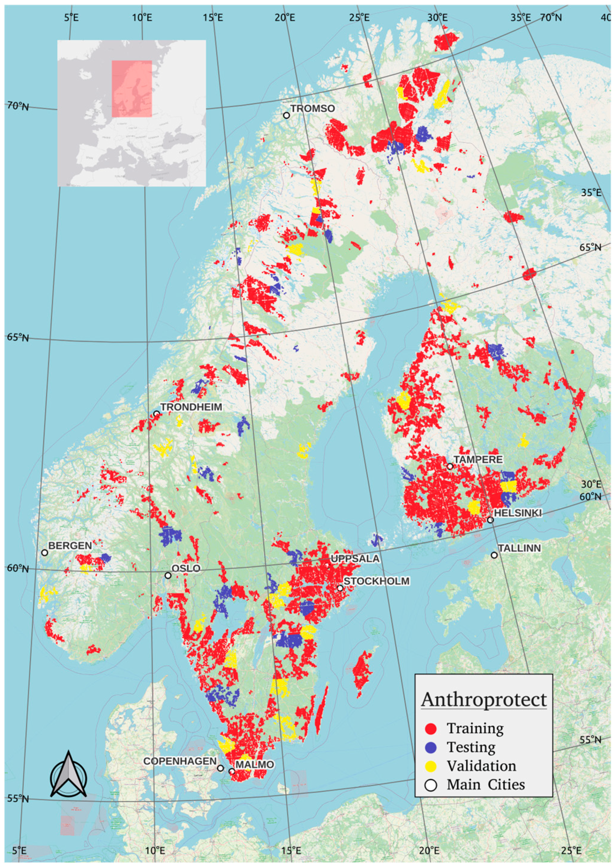
Figure 1. Location of the study area and overall spatial distribution of training, validation, and testing sets for the AnthroProtect dataset.
Land 14 02333 g001
Figure 2. Percentage of CORINE Land Cover classes in the AnthroProtect dataset.
Land 14 02333 g002
Figure 3. Sample tiles from the AnthroProtect dataset: (af) anthropogenic; (g,h) WDPA-Ia; (i,j) WDPA-Ib; (k,l) WDPA-II.
Land 14 02333 g003
Figure 4. Image classification. Impact of different batch sizes: (a) Training accuracy; (b) validation accuracy.
Land 14 02333 g004
Figure 5. Image classification. Impact of different architectures: (a) Training accuracy; (b) validation accuracy.
Land 14 02333 g005
Figure 6. Image classification. Impact of different band setups for medium batch size: (a) Training accuracy; (b) validation accuracy.
Land 14 02333 g006
Figure 7. Image classification. Impact of different band setups for large batch size: (a) Training accuracy; (b) validation accuracy.
Land 14 02333 g007
Figure 8. Semantic segmentation. Impact of different batch sizes: (a) Training accuracy; (b) validation accuracy.
Land 14 02333 g008
Figure 9. Semantic segmentation. Impact of different architectures: (a) Training accuracy; (b) validation accuracy.
Land 14 02333 g009
Figure 10. Semantic segmentation. Impact of different band setups for DeepLabV3: (a) Training accuracy; (b) validation accuracy.
Land 14 02333 g010
Figure 11. Semantic segmentation. Impact of different band setups for FCN: (a) Training accuracy; (b) validation accuracy.
Land 14 02333 g011
Figure 12. Semantic segmentation. Impact of different band setups for U-Net: (a) Training accuracy; (b) validation accuracy.
Land 14 02333 g012
Table 1. Image classification: Calculation time and accuracies for different configurations. N/A = not available.
ArchitectureBatch
Size
Band
Setup
Calculation
Time
Training
Accuracy
Validation
Accuracy
Testing
Accuracy
F1 Score
(Testing Set)
ResNet1864RGB0 d 11 h 5 min99.72%99.04%99.54%99.60%
ResNet1864RGBN0 d 11 h 8 min99.68%82.02%90.41%N/A
ResNet1864Full spectrum0 d 11 h 17 min99.66%99.71%99.79%99.74%
ResNet18128RGB0 d 5 h 58 min99.76%99.37%99.54%99.36%
ResNet18256RGB0 d 3 h 24 min99.80%99.16%99.67%99.54%
ResNet18256RGBN0 d 3 h 13 min99.73%99.46%99.92%99.94%
ResNet18256Full spectrum0 d 3 h 49 min99.73%99.25%99.75%99.88%
ResNet5064RGB1 d 1 h 56 min99.69%99.33%99.79%99.71%
ResNet5064Full spectrum1 d 2 h 12 min99.62%98.95%99.21%98.65%
Table 2. Semantic segmentation: Calculation time and accuracies for different band setups and architectures.
ArchitectureBatch
Size
Band
Setup
Calculation
Time
Training
Accuracy
Validation
Accuracy
Testing
Accuracy
mIoU
DeepLabV32RGB1 d 15 h 3 min74.39%65.54%66.80%87.65%
DeepLabV34RGB1 d 15 h 3 min74.39%65.54%66.80%87.65%
DeepLabV34RGBN1 d 16 h 4 min72.60%64.80%67.72%87.46%
DeepLabV34Full Spectrum1 d 16 h 21 min74.32%66.82%67.19%87.95%
DeepLabV38RGB1 d 15 h 7 min73.46%66.92%66.92%88.28%
FCN4RGB1 d 5 h 0 min70.90%66.62%66.94%88.39%
FCN4RGBN1 d 8 h 28 min71.92%67.79%68.14%89.08%
FCN4Full Spectrum1 d 7 h 12 min74.32%66.82%67.19%87.94%
U-Net4RGB1 d 0 h 7 min67.57%64.23%65.69%87.53%
U-Net4RGBN1 d 1 h 8 min67.73%65.90%66.54%88.48%
U-Net4Full Spectrum1 d 1 h 8 min74.32%66.82%67.19%87.94%
Disclaimer/Publisher’s Note: The statements, opinions and data contained in all publications are solely those of the individual author(s) and contributor(s) and not of MDPI and/or the editor(s). MDPI and/or the editor(s) disclaim responsibility for any injury to people or property resulting from any ideas, methods, instructions or products referred to in the content.