Assessing an Optical Tool for Identifying Tidal and Associated Mangrove Swamp Rice Fields in Guinea-Bissau, West Africa

Abstract

An optical remote sensing approach was developed to identify areas with high and low salinity within the mangrove swamp rice system in West Africa. Conducted between 2019 and 2024 in Guinea-Bissau, this study examined two contrasting rice-growing environments, tidal mangrove (TM) and associated mangrove (AM), to assess changes in vegetation dynamics, soil salinity concentration, and soil chemical properties. Field sampling was conducted during the dry season to avoid waterlogging, and soil analyses included texture, cation exchange capacity, micronutrients, and electrical conductivity (EC_e). Meteorological stations recorded rainfall and environmental conditions over the period. Moreover, orthorectified and atmospherically corrected surface reflectance satellite imagery from PlanetScope and Sentinel-2 was selected due to their high spatial resolution and revisit frequency. From this data, vegetation dynamics were monitored using the Normalized Difference Vegetation Index (NDVI), with change detection calculated as the difference in NDVI between sequential images (ΔNDVI). Thresholds of 0.15 ≤ NDVI ≤ 0.5 and ΔNDVI > 0.1 were tested to identify significant vegetation growth, with smaller polygons (<1000 m²) removed to reduce noise. In this process, at least three temporal images per season were analyzed, and multi-year intersections were done to enhance accuracy. Our parameter optimization tests found that a locally calibrated NDVI threshold of 0.26 improved site classification. Thus, this integrated field–remote sensing approach proved to be a reproducible and cost-effective tool for detecting AM and TM environments and assessing vegetation responses to seasonal changes, contributing to improved land and water management in the salinity-affected mangrove swamp rice system.

1. Introduction

Mangrove Swamp Rice Production (MSRP) in Guinea-Bissau is a traditional agricultural practice that contributes to local food security and the livelihoods of coastal farmers in several West African countries, particularly in Guinea-Bissau [1,2,3]. This system involves transforming mangrove areas for rice cultivation, primarily to capture freshwater, leach excess salts (Na⁺ and Mg²⁺), and reduce soil salinity to improve cultivation conditions [4,5,6].

Farmers convert these forests into MSRP fields through the slashing of mangroves and the construction of earthen dikes and bunds [3,7,8]. The modification of mangrove soils for rice production presents various challenges, including managing high soil salinity and the variability of nutrient concentrations. Nutrients are crucial for maintaining fertility and promoting the growth of healthy rice plants within mangrove ecosystems. Deficiencies or imbalances can significantly reduce rice yields and degrade soil health, underscoring the need for effective soil management practices [9,10]. Additionally, the anthropogenic alteration of these areas requires careful consideration of the environmental and climatic factors that affect soil fertility, water management, and the long-term sustainability of agricultural practices [11,12]. These environmental factors can influence rice productivity, highlighting the importance of understanding the biophysical conditions of mangrove ecosystems [6,13,14].

MSRP is performed in two distinct zones: the associated mangrove (AM) and the tidal mangrove (TM) fields [14]. Tidal fluctuations and salinity gradients influence these areas [3]. There is a notable lack of research on the spatial distribution and concentration of micronutrients within each zone, and no standardized tools exist to distinguish these areas based on their biophysical characteristics. Addressing these knowledge gaps is essential for improving rice field productivity and ensuring the long-term sustainability of agricultural practices in the region.

Remote sensing of land-surface phenology commonly relies on NDVI time series to identify the onset of greening, which marks the early appearance of vegetation [15,16]. High-resolution imagery from PlanetScope (3–5 m) and Sentinel-2 (10–20 m) has proven particularly useful for tracking phenological dynamics, from crown-level changes to landscape-scale vegetation patterns [17,18]. These datasets enable the extraction of key metrics such as the start, end, and duration of the growing season, and they are especially effective for early detection in heterogeneous landscapes, including smallholder fields [19,20]. However, their reliability depends on careful atmospheric correction [21], the construction of time series analysis, and the integration of in situ information such as rainfall patterns and crop management practices [22].

NDVI has also shown high fidelity in capturing leaf-out timing and within-season growth dynamics. Interannual shifts in green-up closely track rainfall onset and precipitation gradients, such as those driven by the Intertropical Convergence Zone (ITCZ) in water-limited regions [23,24,25]. Recent studies demonstrate that NDVI time series can resolve species-specific phenological phases and enable near-real-time change detection [19,20,22,26] when image differencing (ΔNDVI) is applied to radiometrically corrected series [25]. It highlights abrupt greening associated with rainfall or management interventions. Best practices include combining thresholder NDVI/ΔNDVI with multi-date image stacks, noise filtering, and, when available, multi-year intersections to reduce false positives and stabilize onset detection [27,28]. The combination of PlanetScope and Sentinel-2 data enhances the probability of finding cloud-free images, thereby increasing the temporal and spatial availability of data. This approach makes it a practical and operational method for early-season vegetation monitoring.

The specific objectives of this study are as follows: (i) to test a straightforward process for distinguishing associated mangrove (AM) from tidal mangrove (TM) zones within MSRP fields in Guinea-Bissau using frequent high-resolution optical imagery and refine it through calibration and validation using NDVI; (ii) to analyze the concentration of micronutrients within each of these zones. The overall goal of this study is to enhance understanding of nutrient and water management, supporting sustainable agricultural practices in mangrove swamp rice agroecosystems across the West African region. This approach could also be applied to other agroecological contexts that face challenges related to soil salinity and water management.

2. Materials and Methods

2.1. Study Sites and Key Characteristics of the Case Studies

This research was conducted between 2019 and 2024 in Guinea-Bissau, using two case study sites (Figure 1). The study was carried out at the beginning of the rainy season, before rice transplantation. The first site is located in the southern region, in the villages of Cafine-Cafal (11°12′40.4″ N, 15°10′26.7″ W), which have contiguous fields, and the second one in the north, in the village of Elalab (12°14′48.5″ N, 16°26′30.3″ W). Both sites are situated along the country’s coastal zone, an area affected by salinity problems resulting from tidal influence [13,29,30], salt migration from the groundwater [6], and high concentrations of Magnesium (Mg²⁺) and sodium (Na⁺) [31].

Rainfall in Guinea-Bissau exhibits high interannual variability, with the rainy season typically beginning in early June and extending through October [32]. Annual rainfall averages range from approximately 1500 mm in the north to 2500 mm in the south. The onset of rainfall is highly variable in intensity and generally begins in the southern part of the country, gradually advancing northward in response to the movement of the ITCZ [33,34]. Consequently, rainfall typically reaches the northern region later in the season. This part of Guinea-Bissau is classified as moist sub-humid, with an aridity index (AI) of approximately 0.7. In contrast, the southern region experiences markedly wetter conditions, with AI values exceeding 1.0 [35]. According to the Holdridge Life Zone Classification [36,37], the village of Elalab in the North falls within the tropical dry forest zone, while Cafine-Cafal in the South is in the tropical moist forest zone.

MSRP is classified as a rainfed wetland rice ecosystem, being highly vulnerable to both drought and flooding [4]. These areas were originally tidal terraces covered by mangrove forest, which were later transformed into plots for freshwater harvesting and rice cultivation [14]. This transformation was driven by local farmers’ search for more fertile lands to increase rice production and ensure food security for their communities. Rice cultivation is only possible during the free-salt period [6], which depends on the volume of freshwater harvested in the plots.

In agroecological terms, MSRP (“bolanha Salgado” in Creole) occurs in two different environments classified as: (a) tidal mangrove (TM) undergoing direct exposure to tidal dynamics (the rice plots are usually called bolanha de tarrafe in Creole); (b) associated mangrove (AM), adjacent to the TM zone, further inland near the village (the rice plots are usually called bolanha de riba in Creole). The ecology and production conditions of AM and TM fields have been well described in previous articles [14,38,39]. Farmers consider the upland zone of AM plots to be less productive than the TM plots, as they have been cultivated for a more extended period and their fertility has been negatively impacted by shorter rainy seasons and higher air and soil temperatures [39]. Although AM plots still form part of the traditional agricultural landscape, many are being abandoned and replaced by the opening of new, more fertile areas in the mangroves. Only rice varieties with high salinity tolerance can be grown in the TM areas, while less salt-tolerant varieties are cultivated in the AM zones.

2.2. Field Data Collection and Soil Laboratory Analysis

To evaluate the initial condition of soil chemical properties and salinity levels, soil samples were collected during the dry season (May–June 2022). Due to the standing water during the rainy season, sampling was impractical. To ensure consistency and representativeness, sampling grids were established in each village to standardize soil collection. Composite samples were obtained from the 0–25 cm soil layer using a soil auger.

Soil samples were prepared and processed to determine soil texture using the hydrometer method [40,41,42], following the USDA particle size classification. Additionally, cation exchange capacity (CEC) was quantified using the ammonium acetate method [43]. Aluminum (Al) and Iron (Fe) concentrations were determined through oxalate extraction [44,45], while phosphorus (P), Zinc (Zn), copper (Cu), iron (Fe_M3), manganese (Mn), boron (B), and sulfur (S) were measured using the Mehlich-3 extraction method [46]. Cation concentrations were analyzed via inductively coupled plasma mass spectrometry (ICP-MS), following the procedure described by [47]. Electrical conductivity (EC) measurements, initially estimated from a 1:2.5 soil-to-water extract (EC_1:2.5, dS m⁻¹), were converted to saturated paste extract values (EC_e, dS m⁻¹) using the adjustment methodology by [31], which accounts for soil texture effects as outlined in [48].

Automated weather stations were installed at the rice cultivation sites in each village, positioned in open areas free of trees and distant from houses to avoid interference. Each station was equipped with an ATMOS 41 sensor (Meter Environment Products, Pullman, WA, USA), installed on metal poles at a height of two meters and oriented northward. The weather stations were installed in accordance with the manufacturer’s installation guidelines, and data were recorded using the ZL6 datalogger (Meter Group, Pullman, WA, USA), which was configured to log readings every 30 min. Daily rainfall data were continuously collected over the four-year study period.

2.3. Methodology Overview

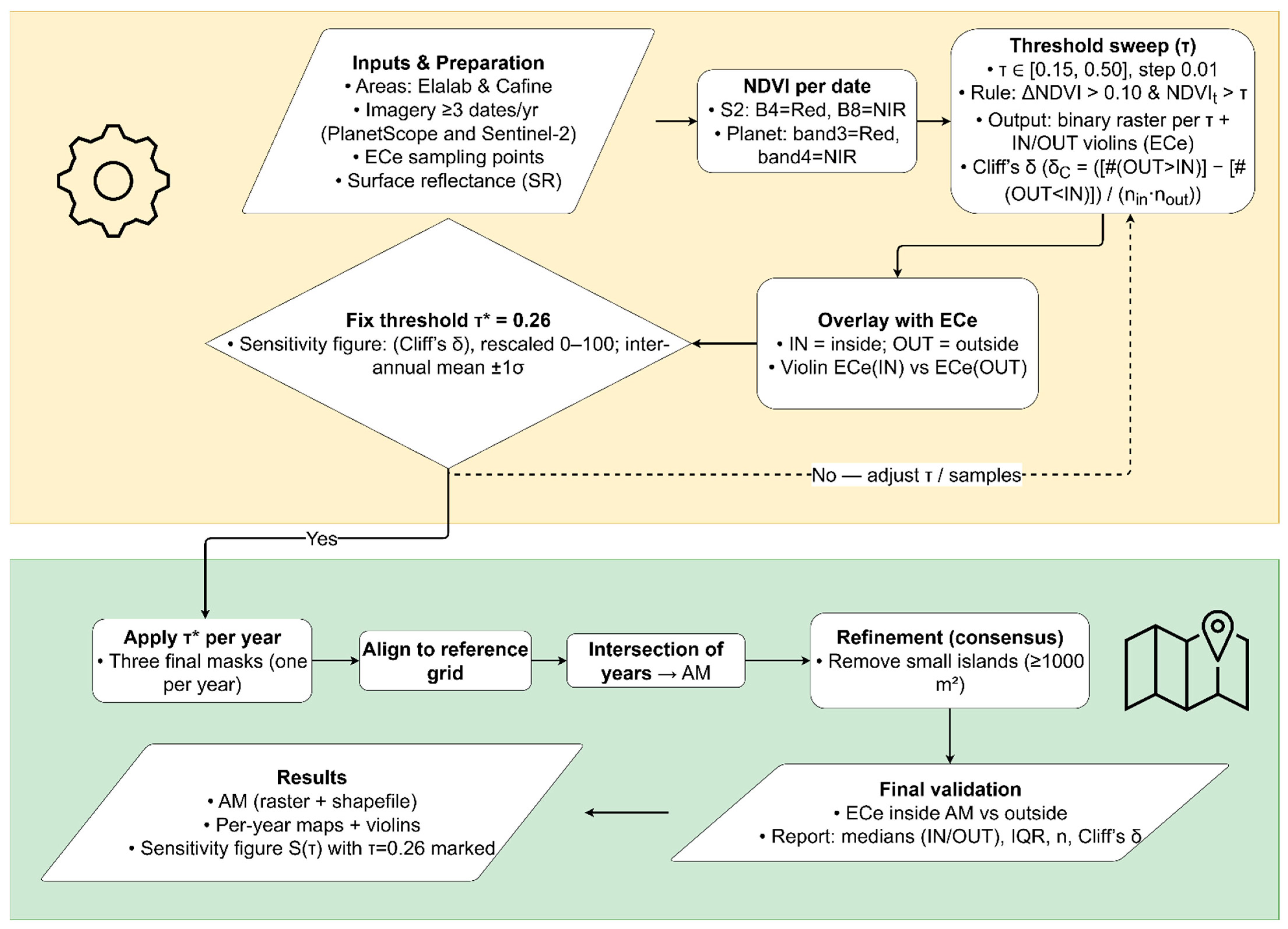
Figure 2 summarizes the workflow to delimit the associated mangrove (AM) zones. The upper panel covers the diagnostic and NDVI-threshold (τ) selection phase: data preparation, per-date NDVI computation, a sweep of τ within (0.15, 0.50) under the rule ΔNDVI > 0.10 and NDVI_t > τ, spatial overlay with Electrical Conductivity of the saturation paste extract (EC_e, dS m⁻¹) points, and inspection of violin plots and metrics until the final threshold τ* is fixed. During this sweep, we also consider Cliff’s Delta, which is a non-parametric effect size measure that quantifies the difference between two groups of observations. Cliff’s Delta calculates the probability that a randomly selected value from one group will be higher than a randomly selected value from another group, minus the probability of the inverse [49,50,51]. Values farther from 0 indicate stronger separation, are robust to non-normality, and are rescaled to 0–100 to enable interannual comparison. This allows us to measure how often EC_e values outside AM exceed those inside AM for each value of τ. In practice, τ candidates were favored when they simultaneously produced (i) a higher median (EC_e_OUT) − median (EC_e_IN), (ii) a positive Cliff’s δ of larger magnitude, and (iii) visually consistent IN/OUT distributions; this guided the choice of τ.

The lower panel illustrates the application and validation phase: applying τ* per year to obtain three binary masks, aligning them to a standard grid, intersecting them to define the AM extent, removing small islands (≥1000 m²) as a cartographic clean-up, and validating the result with the EC_e data (reporting medians, IQR, n, and Cliff’s δ for IN vs. OUT).

2.4. Remote Sensing Data and Calculations

Our approach utilizes optical images containing the red (RED) and near-infrared (NIR) bands, which are heavily influenced by clouds that impede the early appearance of vegetation (Et). Satellite imagery was acquired from PlanetScope and Sentinel-2 (Table 1) due to their high spatial resolution, revisit frequency, and cost-effectiveness in vegetation monitoring [52]. Due to its coverage and resolution, PlanetScope was the primary source of information; however, when more data was required, a search was conducted in the Sentinel-2 database to fill the gaps.

The following steps summarize our approach:

• Image selection
• Vegetation index computation (NDVI)
• NDVI change detection
• Binary classification and vectorization
• Result validation

These steps are further explained in the following subsections.

2.4.1. Image Selection

At least three images per year were used: (i) a dry-season baseline (minimal greenness), (ii) the onset of the rainy season (start of the response window), and (iii) a follow-up about 0.5–one month later (Figure 2). Additional dates were included when they became available to resolve the early appearance of vegetation (Et). The final AM area delineation was computed by intersecting three different years to reduce variability and increase robustness. To mitigate cloud effects, we retained only cloud-free scenes over the study area. This yielded short, clean time series around the key phenological window: Cafine, four dates in 2022 and 2023, plus 2019 Sentinel-2B; Elalab, four dates per season (three in 2021). These series enable the calculation of ΔNDVI and the thresholds at each site.

PlanetScope provided the main time series (3 m, ≈2.9-day revisit) [53]. For Cafine-Cafal in 2019, we utilized Sentinel-2 (10 m, with a temporal resolution of approximately 5–6 days) due to its availability. PlanetScope was used in subsequent years. All imagery within a given year came from the same provider to avoid cross-sensor harmonization. Table 1 lists providers and acquisition dates by area. The satellite images were acquired through the Planet Explorer platform (https://www.planet.com/explorer/, accessed on 30 March 2024), while the red and NIR bands from Sentinel-2 were prepared in Google Earth Engine [54].

Table 1. Characteristics of the satellite data collected.

Village	Provider	Temporal Resolution	Resolution (m)	Year	Date
Cafine-Cafal	Sentinel 2B	6 days	10	2019	05-30
					06-14
					07-04
	Planet Labs	2.9 days	3	2022	05-24
					06-02
					06-10
					06-26
				2023	05-16
					05-23
					06-04
					06-24
Elalab	Planet Labs	2.9 days	3	2021	06-24
					07-04
					08-13
				2022	06-08
					06-22
					07-09
					08-01
				2024	05-31
					06-11
					06-16
					07-14

Source: Planet imagery © 2021–2024 Planet Labs PBC, used under the Education & Research Program license; Sentinel-2 data from the Copernicus Programme [53].

Table 1. Characteristics of the satellite data collected.

Village	Provider	Temporal Resolution	Resolution (m)	Year	Date
Cafine-Cafal	Sentinel 2B	6 days	10	2019	05-30
					06-14
					07-04
	Planet Labs	2.9 days	3	2022	05-24
					06-02
					06-10
					06-26
				2023	05-16
					05-23
					06-04
					06-24
Elalab	Planet Labs	2.9 days	3	2021	06-24
					07-04
					08-13
				2022	06-08
					06-22
					07-09
					08-01
				2024	05-31
					06-11
					06-16
					07-14

Source: Planet imagery © 2021–2024 Planet Labs PBC, used under the Education & Research Program license; Sentinel-2 data from the Copernicus Programme [53].

Finally, it is worth noting that sensors were not mixed within the same season. Each annual series was built from a single sensor (PlanetScope in 2022–2023; Sentinel-2 in 2019). Preprocessing was consistent by sensor (surface reflectance, cloud filtering, NDVI), and thresholds were estimated and applied per site–year–sensor.

2.4.2. NDVI Computation

For each entry of Table 1, orthorectified and atmospherically corrected (surface reflectance) imagery was used to ensure radiometric consistency over time. Then, the Normalized Difference Vegetation Index (NDVI) was calculated from the NIR and RED bands of each image (Equation (1)) [55]:

$$\mathrm{N}\mathrm{D}\mathrm{V}\mathrm{I}=(\mathrm{N}\mathrm{I}\mathrm{R}-\mathrm{R}\mathrm{E}\mathrm{D})/(\mathrm{N}\mathrm{I}\mathrm{R}+\mathrm{R}\mathrm{E}\mathrm{D}),$$

(1)

2.4.3. Change Detection Method for Early Appearance of Vegetation (Et)

Our approach assumes that when the rainy season starts, the associated mangrove vegetation grows at a higher rate than in other mangrove areas. This behavior is based on the fact that vegetation in areas with low soil salinity conditions can grow first, followed by areas with high salinity, which implies a lag in their growth due to the dissolution of salt in the soil with rainfall.

This process was designed as a simple approach involving NDVI, which associates vegetation vitality with a normalized difference between the NIR and RED bands, as described in Equation (1) [55]. A time series change detection was performed by subtracting the previous NDVI image (NDVI〗_(t−1)) from the current analysis (NDVI〗_t) (Equation (2)).

$$∆\mathrm{N}\mathrm{D}\mathrm{V}\mathrm{I}={\mathrm{N}\mathrm{D}\mathrm{V}\mathrm{I}}_{\mathrm{t}}-{\mathrm{N}\mathrm{D}\mathrm{V}\mathrm{I}}_{\mathrm{t}-1},$$

(2)

A pixel was flagged as an early-appearance candidate at the earliest time t satisfying two simple rules:

i.

NDVI_t > τ (NDVI threshold), and

ii.

ΔNDVI_t > δ (minimum positive change).

The NDVI values indicative of sparse vegetation are generally associated with lower ranges, typically falling between 0.2 and 0.4, as supported by studies that classify and analyze vegetation density using NDVI thresholds or ranges [15,56]. Furthermore, a default value of 0.1 was set for δ, as a pixel with an NDVI value of 0.4 is more likely to represent an area with vegetation, as indicated by the threshold values computed by [57].

2.4.4. Per-Year Threshold Sweep and Diagnostics

For each year and area, a grid of τ ∈ [0.15, 0.50] (step size 0.01) with δ = 0.10 fixed was evaluated. For everyτ, three products were generated: the binary early-appearance raster, overlaid EC_e field samples: IN (inside mask) and OUT (outside), and produced plots of EC_e (IN) vs EC_e (OUT), recording medians, Interquartile Range (IQR), sample sizes, and mapped area fraction.

To quantify the separation between EC_e inside and outside the candidate mask, we used Cliff’s delta, with the exact orientation implemented in the code. Let X be the set of EC_e values for IN points (size n_IN) and Y be the set for OUT points (size n_OUT). Then Cliff’s delta δ is defined as Equation (3):

$${\delta }_c={\displaystyle \frac{\#\left\{\left(x\in {\rm X},\gamma \in Y\right):x>y\}-\#\left\{\left(x\in {\rm X},\gamma \in Y\right):x<y\}\right.\right.}{\left|X\right|\left|Y\right|}} ϵ[-\mathrm{1,1}],$$

(3)

With this sign convention, δ > 0 indicates that IN tends to have larger EC_e values than OUT, δ < 0 the reverse, and δ ≈ 0 implies substantial overlap. This matches the comparison logic used in the code (binary searches over sorted OUT values to count the two types of pairs).

2.4.5. Threshold Selection and Multi-Year Integration

The final selected threshold τ* was chosen to maximize separation between areas outside the AM and regions inside the AM, based on the EC_e, subject to plausibility constraints. Per year “y”, the primary metric was:

$${\Delta }^y\left(\tau \right)={\mathrm{m}\mathrm{e}\mathrm{d}\mathrm{i}\mathrm{a}\mathrm{n}\left(\mathrm{E}{\mathrm{C}}_{\mathrm{e}}\mathrm{O}\mathrm{u}\mathrm{t}\right)}^{\mathrm{y}}-{\mathrm{m}\mathrm{e}\mathrm{d}\mathrm{i}\mathrm{a}\mathrm{n}\left(\mathrm{E}{\mathrm{C}}_{\mathrm{e}}\mathrm{I}\mathrm{n}\right)}^{\mathrm{y}},$$

(4)

Separation across years was summarized by Equation (5).

$$s\left(\tau \right)={\overline{\mathrm{x}}}_{\mathrm{O}\mathrm{v}\mathrm{e}\mathrm{r}\mathrm{y}\mathrm{e}\mathrm{a}\mathrm{r}\mathrm{s}}\left\{{\Delta }^{\mathrm{y}}\left(\mathsf{\tau }\right)\right\}$$

(5)

Thresholds with IN/OUT samples were discarded. The selected τ* was the value giving a significant, consistent separation with a reasonable extent and minimal overlap in violins. This τ* was then applied to each year to produce three final masks. The final selected τ value was 0.26.

The final “associated mangrove (AM)” map was derived by aligning all per-year masks to a reference grid and taking their intersection, yielding areas that respond consistently to the earliest vegetation appearance across years.

2.5. Validation of the Result

The validation relied on classifying field soil samples as IN_AM (inside the final AM polygon) or OUT_AM (outside). This enabled a direct comparison of EC_e distributions via violin plots and summary statistics—medians, interquartile range (IQR), and sample size (n)—for both groups.

For each τ and year, we (i) computed the binary early-appearance mask, (ii) assigned each EC_e sample to IN/OUT, and (iii) quantified the separation between groups with Cliff’s delta δ (together with medians, IQR, and n). Importantly, δ was computed following our implementation, where the IN samples are the reference set and the OUT samples are the comparison set; under this convention, δ>0 indicates that EC_e tends to be higher in OUT than in IN, which is the direction expected if AM exhibits relatively lower soil salinity. We examined whether (a) the sign and magnitude of δ were stable near the chosen range, (b) the IN/OUT medians were consistently ordered (OUT > IN for EC_e), and (c) the classified area varied plausibly with τ. These diagnostics were summarized across years to assess robustness around the ultimately selected threshold τ.

Finally, we conducted visual validation, overlaying the AM polygon on the imagery and field context to confirm spatial plausibility. Together, the statistical diagnostics (including Cliff’s δ with the stated orientation), distribution summaries, and visual checks support the internal consistency of the results and the selected threshold.

2.6. Spatial Post-Processing

The binary raster was converted to a vector file, and a noise removal process was applied. The noise removal involved removing polygons smaller than 1000 m², which is approximately the area of a typical 9 × 9 pixels. Finally, the change detection methodology steps were implemented in Python 3.10. The workflow relied on widely used open-source libraries, including “NumPy (1.24.1)” for numerical computation, “Rasterio (1.13.10)” for raster reading, writing, and masking, “GeoPandas (1.0.0)” for vector data processing and coordinate reference system management, “Matplotlib (3.9.0)” for visualization, “Shapely (2.0.4)” for geometry handling, and “Pandas (2.2.2)” for tabular data analysis [58].

The complete and reproducible source code, along with example datasets and a Jupyter Notebook (.ipynb) (https://jupyter.org/) illustrating the workflow, is provided as Supplementary Materials (See GitHub (3.5.3) repository).

2.7. Statistical Analysis

Once the areas were delineated using the intersection analysis, specific sampling locations were identified within both the AM and TM zones. This spatial separation enabled the independent physicochemical analysis of soils from each area, allowing for the validation and distinction of the two agroecological zones.

Soil chemical parameters were evaluated for normality using the Shapiro–Wilk test. Since most variables did not meet the assumption of normality, the non-parametric Wilcoxon rank-sum test (equivalent to the Mann–Whitney U test) was applied to detect significant differences between groups. A significance level of α = 0.05 was used. Results were considered statistically significant when p-values were below 0.05. Graphical representations used asterisks to indicate levels of significance as follows: α < 0.05 (*), α < 0.01 (**), and α < 0.001 (***). All statistical analyses were conducted using R software version 2024.04.1 [59].

3. Results

3.1. Rainfall Timing for NDVI Windows and Image Selection

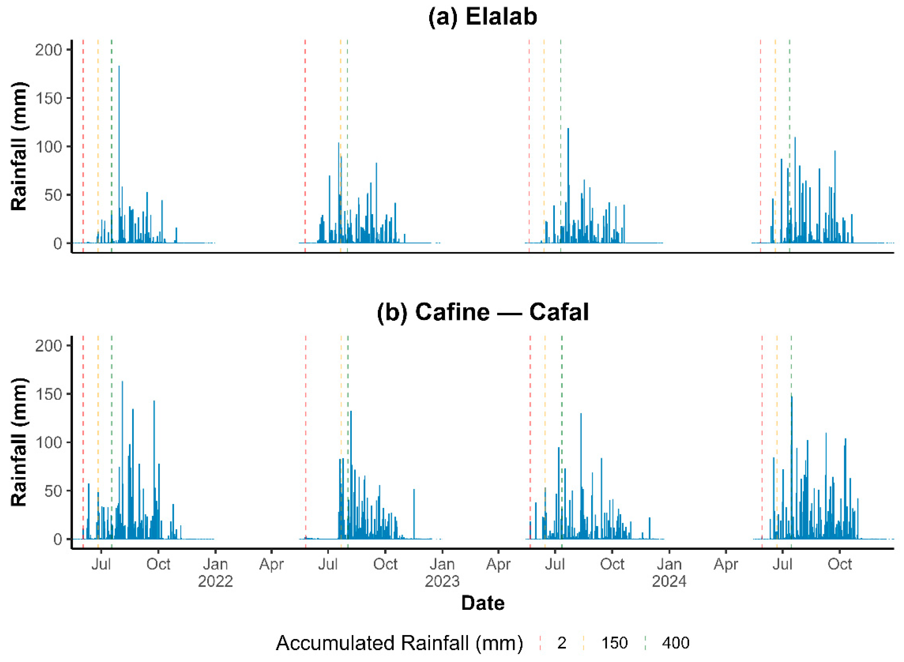
Rainfall proved to be a reliable indicator for identifying areas with lower soil salinity, as salt-intolerant weeds exhibit rapid growth following the onset of the rainy season. In this study, rainfall records were used to determine the optimal timing for acquiring the PlanetScope and Sentinel-2 imagery (Figure 3). Three reference stages were defined: (i) a baseline with 2 mm of rainfall, (ii) an early period with 150 mm, and (iii) a late rainy period with 400 mm. The last stage was critical, as in MSRP plots, the accumulated freshwater dilutes soil salts, marking the beginning of the locally recognized free-salt period, which allows rice cultivation [6].

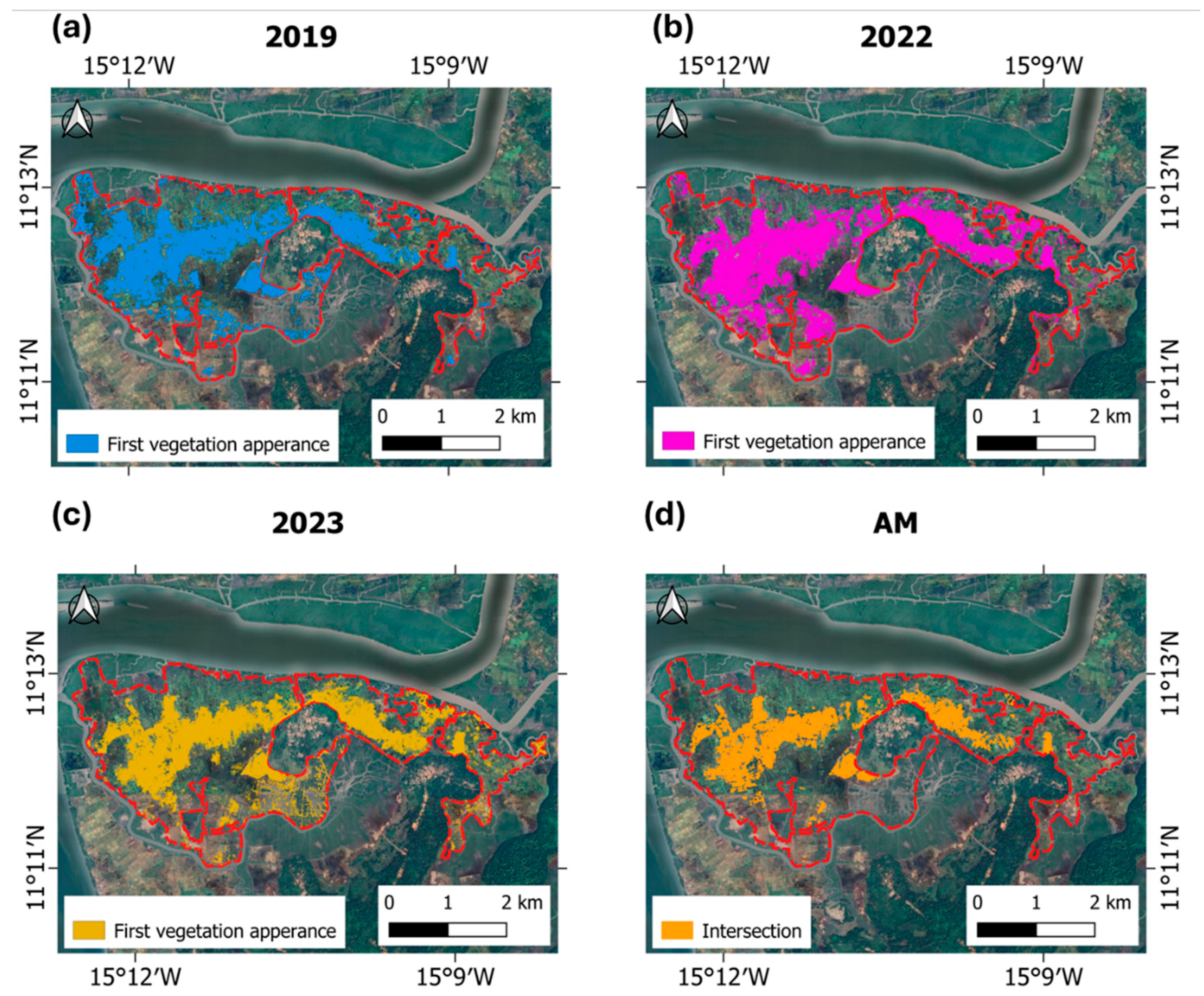
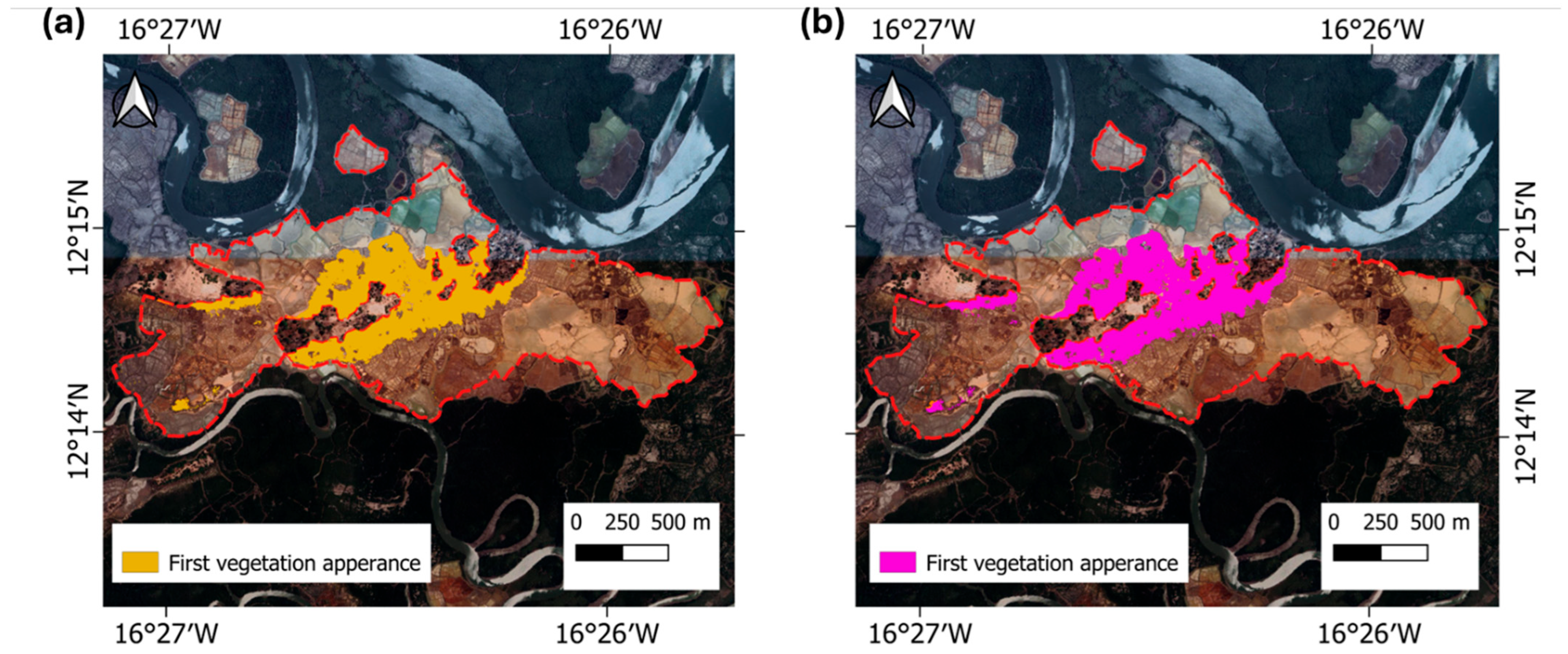
Between 2021 and 2024, rainfall patterns exhibited substantial variability (Figure 3). The Elalab site consistently received lower and more irregular rainfall compared to Cafine─Cafal (Figure 3). In both villages, an accumulated rainfall of approximately 150 mm was recorded between the end of June and the beginning of July. July was used as the observation month for measuring vegetation reflectance in the associated mangrove areas (Figure 4 and Figure 5). To illustrate the early-greenness window at the site scale, Figure 4 summarizes the first vegetation appearance and the multi-year intersection for Cafine–Cafal.

An analogous sequence for Elalab is provided in Figure 5, using July acquisitions for the corresponding years.

3.2. Validation of NDVI Thresholds for Early Vegetation, Salinity Zoning, and Site Classification

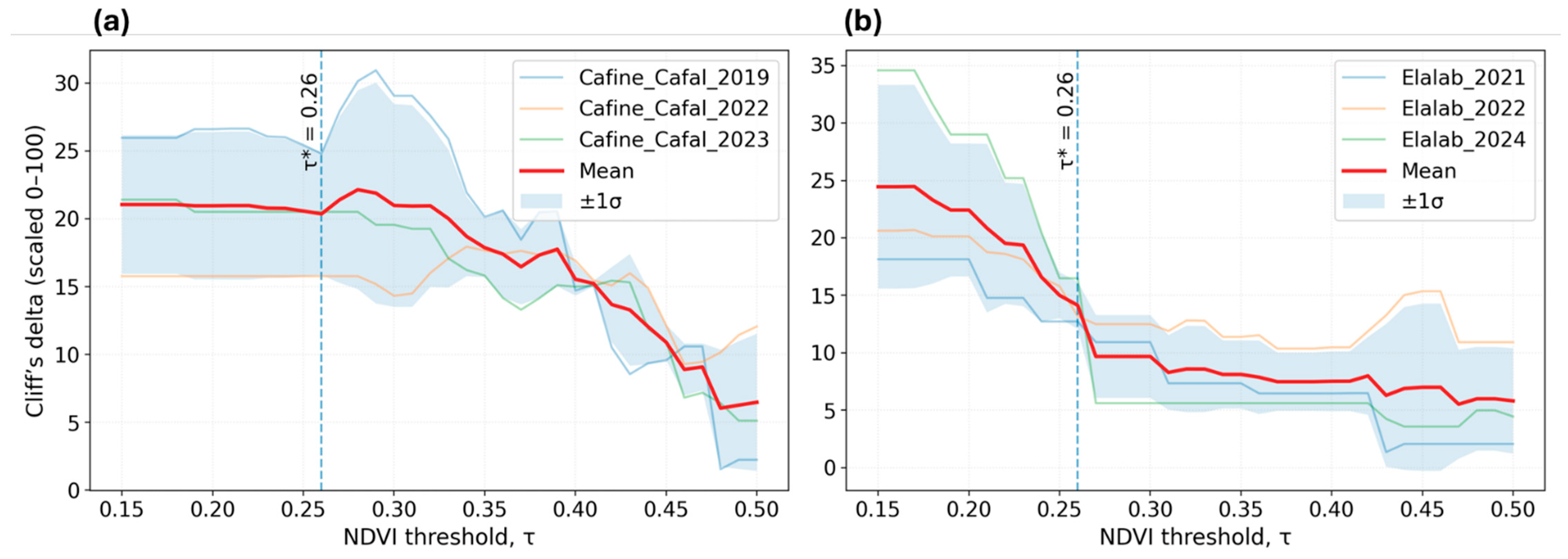
It was found that early vegetation and salinity zoning based on NDVI responded best at a threshold of 0.26, identified as the optimal value considering the workflow and the validation. For instance, in Cafine-Cafal (Figure 6a), Cliff’s delta (δ) stays relatively stable up to an NDVI value (τ) of 0.32. However, when τ is 0.26, it presents a more precise mapping result, with no apparent improvement when this value increases.

In contrast, in Elalab, a τ of 0.26 represents an inflection point with a sharp decline in δ values, after which the curve plateaus, indicating no further change with a higher τ value (Figure 6b).

Additionally, visual inspection confirmed that there is no improvement in AM detection after this threshold (Figure 7 shows no apparent difference between τ values of 0.26 and 0.32). To ensure consistency and compatibility across sites, we therefore fixed the final threshold at τ = 0.26 for both villages (δ > 0 implies EC_e_OUT tends to exceed EC_e_IN).

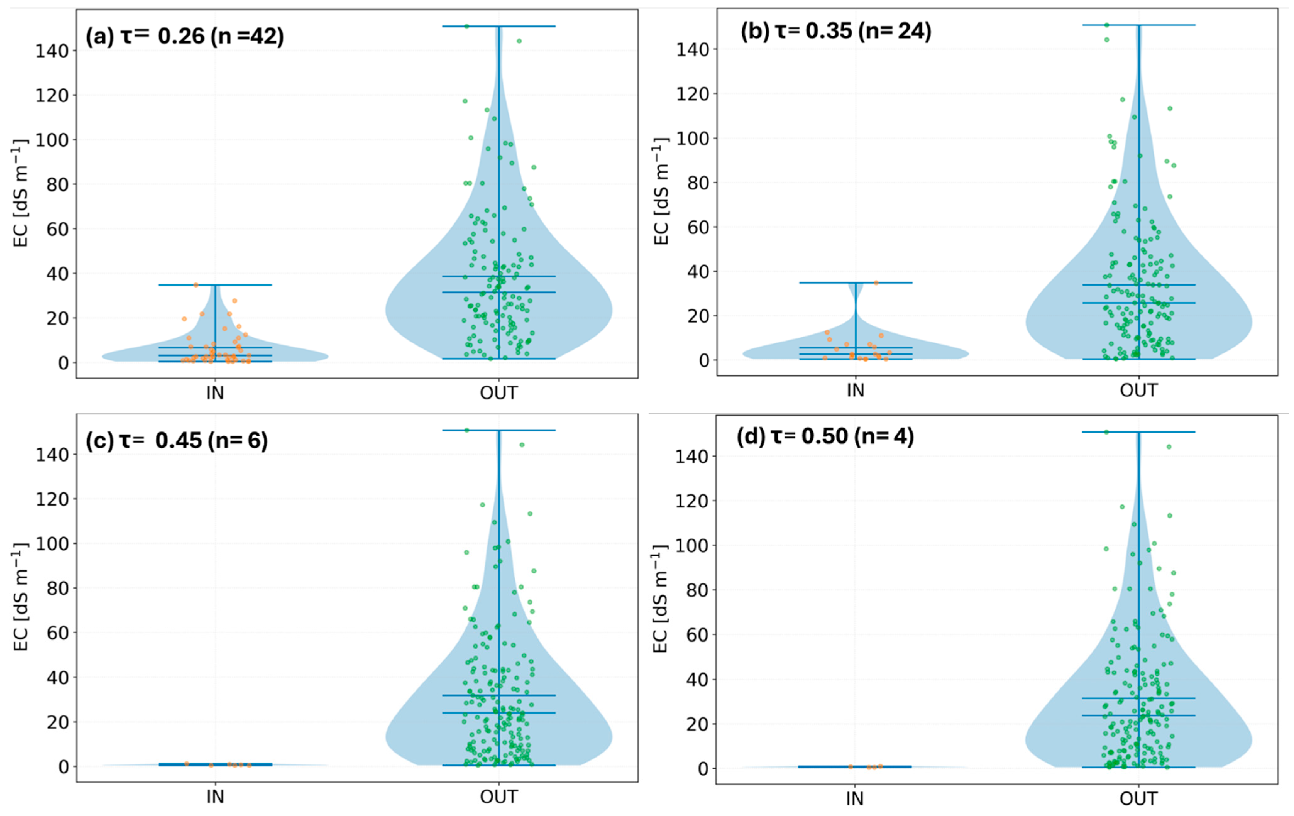
Zoning outcomes varied depending on the presence of sampling sites, with violin plots showing a significant reduction in variability (see Figure 8 for Cafine-Cafal; additional figures on GitHub display the same type of image and trend for the case of Elalab). This calibration step enables the application of the optimal threshold across satellite images from different years, including Sentinel-2 data from 2019. The results clearly demonstrate that this tool can be applied in diverse regions of the country, opening the possibility of extending its use to other West African countries to identify hypersaline zones in MSRP sites.

Finally, the results were based on first accurately identifying the AM areas, then the TM. The boundaries of both regions are shown in Figure 9, which displays the spatial distribution of these areas.

3.3. Comparison of the Sites’ Nutrients

Soil texture also exhibited significant differences in clay and silt content between villages, in both TM and AM sites (Figure 10). TM plots showed higher cation exchange capacity (CEC) compared to AM plots (

Table 2. Statistical comparison analysis of soil physicochemical parameters in associated mangrove (AM) and tidal mangrove (TM).

Village	Variables	Units	Mean TM	Mean AM	W	p Value
Elalab n = 99	ECe	dS m−1	106.53	9.09	1096.5	<0.001
	Sand	Index	0.56	0.86	172.0	<0.001
	Clay		0.12	0.08	890.0	0.003
	Silt		0.32	0.06	1014.5	<0.001
	CEC+	cmol(+) Kg−1	9.94	3.15	905.0	0.002
	Fe *	%	0.24	0.08	903.0	0.002
	P	mg L−1	15.24	14.36	770.0	0.079
	Zn		1.04	0.84	752.5	0.114
	Cu		1.33	0.94	818.5	0.006
	Fe_m3		309.31	277.71	666.5	0.476
	Mn		3.42	1.44	914.0	0.001
	B		6.30	0.78	1103.5	<0.001
	S		740.14	81.43	1081.0	<0.001
Cafine-Cafal n = 183	ECe	dS m−1	38.16	6.02	4682.5	<0.001
	Sand	Index	0.26	0.27	2664.5	0.793
	Clay		0.27	0.33	2024.5	0.045
	Silt		0.47	0.40	3698.5	<0.001
	CEC+	cmol(+) Kg−1	24.90	24.78	2307.0	0.316
	Fe *	%	0.82	0.63	3460.0	0.002
	P	mg L−1	17.05	8.63	4205.5	<0.001
	Zn		2.66	1.79	3566.5	0.001
	Cu		0.96	0.83	2971.5	0.036
	Fe_m3		485.53	446.97	3031.5	0.118
	Mn		19.53	15.46	2871.5	0.318
	B		2.91	1.45	4493.0	<0.001
	S		395.99	165.09	4090.0	<0.001

CEC in ammonium acetate; * Fe in calcium oxalate; Fe_m3 = iron in the Mehlich-3 soil extraction method. Soil samples were collected during the dry season (May–June 2022).

). In the northern regions, the mean CEC was lower (means, TM = 9.94 cmol(+) Kg⁻¹, AM = 3.15 cmol(+) Kg⁻¹) than in the southern region (means, TM = 24.9 cmol(+) Kg⁻¹, AM = 24.8 cmol(+) Kg⁻¹). CEC is primarily composed of exchangeable cations, including Ca, Mg, K, and Na [43,60,61]. In Elalab, TM soils contained a higher concentration of exchangeable bases compared to AM soils (Table 2). In Cafine–Cafal, no significant differences were found, and the mean values were similar across both sites (Table 2).

Considering the soil data and results, the analysis of P, Cu, B, and S revealed significantly (α < 0.05) higher concentrations in TM compared to AM (Table 2).

4. Discussion

4.1. Rainfall Variability, Observation Windows, and Cloud Constraints

In semi-arid regions, vegetation exhibits rapid responses to short, intense rainfall events, resulting in pronounced interannual variability [62]. Then, rainfall data can be used to predict periods of high vegetation activity (Figure 3), which are optimal for satellite image acquisition [63]. Thus, the three reference stages (Section 3.1) provided a comparative framework for detecting vegetation reflectance through NDVI, enabling assessment of plant growth in associated mangrove environments.

Between 2021 and 2024, rainfall patterns exhibited substantial variability, likely driving differences in vegetation cover dynamics. This interannual variability in the country has been reported by [32,33]. The Elalab site consistently received lower and more irregular rainfall compared to Cafine-Cafal (Figure 3). However, in both villages, an accumulated rainfall of approximately 150 mm was recorded between the end of June and the beginning of July, which was sufficient to break weed dormancy and trigger initial growth. Consequently, July was identified as the optimal month for measuring vegetation reflectance, as it marks the emergence of the first significant ground cover in the associated mangrove areas (Figure 4 and Figure 5). Incorporating time windows of 20–40 days for merging satellite observations can further enhance the accuracy of vegetation monitoring, providing more frequent and reliable information [64]. The representative month then changes between the two villages, with early vegetation appearing in June and July for Cafine-Cafal and Elalab, respectively.

Regarding cloud cover, even though filtering ensured the use of cloud-free scenes and allowed the necessary images to be assembled for analysis, persistent cloudiness can reduce the effective temporal frequency and, in specific cases, prevent the capture of phenological events between images. This aspect has also been documented in the literature; for example, [65] reports temporal gaps due to frequent cloud cover in Sentinel-2 time series and notes that persistent cloudiness reduces the quality of optical data.

4.2. NDVI Usage and Threshold Calibration

The NDVI is the most widely used index for detecting land-cover changes through remote sensing. For instance, NDVI application has been documented in a wide range of vegetation studies, including assessments of desert vegetation cover [66], transformations of vegetation types [67], responses of vegetation growth and cover to climatic factors [68], and the differentiation of primary from secondary forest [69]. In our study, it was found that NDVI can also provide critical information for identifying AM and TM sites, which are characterized by higher salinity (Figure 4 and Figure 5). Soil salinity (EC_e) in TM and AM sites presents highly significant differences (α = 0.001) (Figure 10). This finding validates the management strategies adopted by farmers in Guinea-Bissau [11,12], who select rice varieties for TM and AM plots with different tolerance levels to soil salinity and fertility conditions [39].

The results also show that the choice of threshold in NDVI is a critical aspect in phenological detection. In this sense, the variation in the index was explored in a range of τ ∈ [0.15, 0.50] with increments of 0.01, allowing for evidence on how slight differences in the threshold can modify the detection capacity of AM zones. This finding aligns with what has been reported in previous studies, such as [70], who applied dynamic threshold approaches to detect sowing and harvesting dates in maize and soybean, and with works that have used the value of 0.35 as a baseline to exclude non-agricultural lands (pixels with maximum NDVI lower than that value). The final threshold of 0.26 selected in this study is explicitly adjusted to the context of early vegetation growth in MSRP. Complementarily, [65] used relative threshold increments of 69% in Sentinel-2 and 63% in MODIS with respect to a 4-year NDVI mean to detect the onset of growth in Arctic tundra, which reinforces the idea that thresholds should be calibrated according to cover type, sensor, and environmental conditions, ensuring robust and transferable phenological estimates. Another example is the case of [71], which considered a relative threshold of 10% of the Enhanced Vegetation Index (EVI) amplitude, based on the annual maximum and minimum, to monitor phenological stages in rice. The authors tested different values before settling on 10%, reinforcing that an explicit, calibrated threshold can be appropriate for operational phenology detection.

This rigorous process enabled us to calibrate the model to accurately distinguish between saline and non-saline areas, in line with field observations. Although several of these previous results come from cropland studies, the underlying principle—using an explicit, calibrated NDVI rule to detect the onset of greenness or vegetation appearance with the start of the rainy season—is directly transferable here.

A second line of evidence came from Cliff’s delta (δ), a non-parametric effect-size measure that quantifies stochastic dominance between two groups. Operationally, in our study, δ(τ) captures how often EC_e values outside AM exceed those inside AM for each candidate τ. Values farther from zero indicate stronger separation and are robust to non-normality and unequal variances. We used δ alongside the median difference [median(EC_e_OUT) − median(EC_e_IN)] and visual inspection of violin plots to guide selection of τ*: candidates were favored when they simultaneously produced a larger positive δ, a higher median separation, and spatially plausible AM extents. Similar uses of Cliff’s delta to assess the magnitude of differences in NDVI-derived productivity/phenology metrics are reported in [50] and as a criterion for identifying the vegetation index that best separates forest-type classes before Sentinel-2 modeling [72].

The validation process also included visual verification of weed presence, ensuring that NDVI-based identification was supervised and consistent with field observations, as recommended [73,74]. Temporal analysis, such as change detection, varied across years because rainfall intensity influenced whether weed growth occurred more rapidly or gradually [75]. This phenomenon highlighted the need to complement the early appearance of the vegetation tool with rainfall data, particularly in the study sites. Then, this consistency reinforces the applicability of NDVI for vegetation monitoring, provided that the results are validated with field observations [15,73].

Furthermore, to incorporate the intersection of identified zones, it was necessary to first correctly distinguish the AM areas, followed by the TM (Figure 9). Based on these findings, using at least three years of imagery is recommended to achieve robust calibration and reliable site identification of salinity (Figure 4 and Figure 5). For instance, long-term NDVI analyses have proven essential for validating vegetation trends [76], while multi-temporal salinity mapping in West Africa underscores the value of extended observation periods [77].

4.3. Cross-Sensor Considerations

Due to differences in spectral response and resolution, absolute NDVI values are not directly interchangeable between sensors; consequently, threshold selection may require specific adjustments for each sensor. The literature has documented that the optimal threshold may differ between sensors (e.g., Sentinel-2 vs. MODIS) due to non-equivalent red and NIR bands, resulting in different NDVI levels between platforms [65]. In this study, we did not mix sensors within a season. The threshold was estimated and applied separately for each site, year, and sensor. Additionally, the multi-year intersection operates on binary masks, prioritizing persistent spatial patterns over absolute levels and mitigating possible biases between sensors. As shown in Figure 7, the detection process operates safely within a threshold range from 0.26 to 0.32.

4.4. Management Implications for MSRP

Water management in TM plots must be strictly efficient due to the high concentration of salts. MSRP requires adequate dilution of soil salinity to enable rice growth and grain formation. The generated maps provide valuable guidance for identifying areas where large plots can be subdivided into smaller ones to improve freshwater harvesting [13]. In contrast, AM sites benefit from taking advantage of the first rains to establish a rice nursery, combined with the application of green manure and organic fertilizer [39]. This practice promotes the early development of seedlings, thereby reducing waiting times for transplanting into TM plots. Such integration allows farmers to use harvested freshwater more efficiently.

The results show that P, Cu, B, and S were significantly higher in TM compared to AM (Table 2). This represents the first evidence that soil fertility preferences in these agroecosystems are also linked to the high micronutrients concentrations. Considering the seeding practices as well, this pattern may reflect that AM fields in the south have been more recently cultivated, receive more rainfall, and are therefore more fertile than those in the north of the country. Taken together, these results provide evidence that micronutrient availability is likely to influence soil-use preferences in the MSRP system.

Regarding soil texture, the clay, sand, and silt contents differed significantly between villages in both TM and AM areas (Figure 10). This is closely linked to apparent soil fertility [78,79]. The comparison confirms the results obtained from the early vegetation zonation based on the NDVI threshold, as it effectively differentiates between sites. These results support observations of [3] and [1], as Northern farmers prefer to plant Oryza glaberrima in TM plots due to its tolerance to soil salinity. Although P is one of the most critical nutrients for rice growth and productivity [80,81], further research is required to assess organic carbon, carbon stocks, and nitrogen dynamics in these sites.

The differentiation of micronutrient availability between TM and AM sites carries essential implications for rice productivity and management in MSRP. Phosphorus, for instance, is critical for root development, biomass accumulation, and grain yield. At the same time, high soil organic carbon content can further enhance nutrient uptake and improve P-use efficiency in lowland rice [81]. Likewise, the higher CEC observed in TM plots indicates greater potential for nutrient retention, although this must be carefully managed to avoid salinity-induced imbalances [61]. Soil fertility in MSRP fields is influenced by texture and microbial activity. Finer-textured soils generally support higher enzymatic activity and microbial diversity, thereby improving nutrient cycling under saline stress [78]. Recent studies in Guinea-Bissau further demonstrate that mangrove soils exhibit distinct fertility dynamics shaped by agroecological conditions and local practices [38,39], reinforcing the need for site-specific nutrient strategies. When combined with advances in soil salinity diagnostics [31], these insights suggest that integrating nutrient and water management [6] can simultaneously enhance soil fertility and improve water use efficiency. Such spatially explicit approaches enables farmers to optimize plot selection and management practices, ultimately increasing rice yield and promoting sustainable land use within the MSRP fields.

4.5. Considerations Regarding the Model and Research Gaps

The reliability of NDVI-based analyses is influenced by several limitations that must be considered when applying the technique to salinity zoning and site classification in MSR fields. Cloud cover, which is frequent in West Africa during the rainy season, often interferes with the detection of early vegetation signals. This situation requires searching in extensive image archives to filter out cloud-contaminated scenes and retain only the most precise observations. Additionally, NDVI values can be influenced by atmospheric conditions and sensor viewing angles, underscoring the importance of careful calibration and validation against field data [82]. In addition, it is pertinent to consider the diversity of approaches, dynamic thresholds for sowing and harvesting dates [70], and relative thresholds, such as seasonal NDVI percentages [65], which highlight a lack of methodological standardization. Our findings using a locally adjusted value (0.26) reinforce the need to evaluate the transferability of thresholds across crops and ecosystems to move toward more consistent and comparable applications. It is important to note that the threshold obtained should be interpreted as specific to the site and sensors considered. Effective threshold values vary with the sensor and context; for example, in [65], the onset of growth was defined differently for Sentinel-2 and MODIS, attributed to differences in spectral ranges/bands. Similarly, in [70], phenological detection of planting and harvesting is based on dynamic thresholds that are adjusted and validated using local data. Taken together, this evidence supports τ = 0.26 as a local operational threshold for our sites and sensors. The approach applied in this study, potentially transferable to other regions or crops, must be adapted to local contexts.

Future research should also explore the integration of NDVI with complementary indices to improve ecological assessments. For instance, radar vegetation indices (RVI), based on RADAR, can penetrate clouds and provide structural information, while photochemical reflectance indices (PRI) offer insights into photosynthetic activity and stress responses [83,84].

The higher temporal resolution of PlanetScope (3–5 m) compared to Sentinel-2 (10–20 m) is particularly valuable under persistent cloud cover, as it increases the likelihood of capturing usable imagery during critical growth stages [62]. These considerations underscore the importance of multi-sensor strategies and methodological refinement in enhancing early-season monitoring and improving the robustness of site classification models. Furthermore, integrating morphological features with spectral and textural indicators through machine learning techniques [85] could complement future studies focused on monitoring rice cultivation in MSRP.

5. Conclusions

The integration of field data and remote sensing performed in this study enabled the effective identification of associated mangrove (AM) and tidal mangrove (TM) areas, despite spatiotemporal variability. Also, this approach allowed us to analyze micronutrient concentrations in both areas. The developed methodology is straightforward, reproducible, cost-effective, and operational, enabling differentiation between areas of high and low salinity, as well as assessing vegetation responses to seasonal changes.

NDVI, a widely recognized and validated index in remote sensing studies, has proven to be a crucial tool for monitoring vegetation dynamics, enabling the accurate detection of significant changes in vegetation cover over time. The use of NDVI, combined with field data, enabled the establishment of robust thresholds and the validation of mangrove swamp rice field zoning, providing a reliable basis for exploring the AM and TM ecologies with a straightforward approach.

The parameter optimization yielded a locally adjusted NDVI threshold of 0.26. Selected via a multi-year sweep and external validation against EC_e (including Cliff’s delta and sensitivity diagnostics), this threshold underpins the final AM mapping. It supports the interpretation of nutrient and water conditions, offering practical guidance for sustainable management in mangrove swamp rice agroecosystems. The workflow and intersection of multitemporal satellite information within the MSRP fields provide a transferable framework for regions with similar agroecological characteristics.

Nevertheless, the need to deepen the methodology under different environmental scenarios and to explore the integration of other vegetation indices and sensors, including those capable of penetrating cloud cover, is recognized to improve accuracy and broaden the scope of these types of studies in the West African countries’ MSRP ecosystems.

References

1. Temudo, M.P. Inovação e Mudança Em Sociedades Rurais Africanas Gestão de Recursos Naturais, Saber Local e Instituições de Desenvolvimento Induzido Estudo de Caso Na Guiné-Bissau. Ph.D. Thesis, Universidade Técnica de Lisboa, Lisbon, Portugal, 1998. [Google Scholar]
2. Soullier, G.; Demont, M.; Arouna, A.; Lançon, F.; Mendez del Villar, P. The State of Rice Value Chain Upgrading in West Africa. Glob. Food Sec. 2020, 25, 100365. [Google Scholar] [CrossRef]
3. Carney, J. Black Rice: The African Origins of Rice Cultivation in the Americas; Harvard University Press: Cambridge, MA, USA, 2001; Volume 1. [Google Scholar]
4. Balasubramanian, V.; Sie, M.; Hijmans, R.J.; Otsuka, K. Increasing Rice Production in Sub-Saharan Africa: Challenges and Opportunities. Adv. Agron. 2007, 94, 55–133. [Google Scholar] [CrossRef]
5. Sylla, M.; Stein, A.; van Breemen, N.; Fresco, L.O. Spatial Variability of Soil Salinity at Different Scales in the Mangrove Rice Agro-Ecosystem in West Africa. Agric. Ecosyst. Environ. 1995, 54, 1–15. [Google Scholar] [CrossRef]
6. Garbanzo, G.; do Rosário Cameira, M.; Paredes, P.; Temudo, M.; Ramos, T.B. Modeling Soil Water and Salinity Dynamics in Mangrove Swamp Rice Production System of Guinea Bissau, West Africa. Agric. Water Manag. 2025, 313, 109494. [Google Scholar] [CrossRef]
7. Temudo, M.P. Planting Knowledge, Harvesting Agro-Biodiversity: A Case Study of Southern Guinea-Bissau Rice Farming. Hum. Ecol. 2011, 39, 309–321. [Google Scholar] [CrossRef]
8. Temudo, M.P.; Cabral, A.I. The Social Dynamics of Mangrove Forests in Guinea-Bissau, West Africa. Hum. Ecol. 2017, 45, 307–320. [Google Scholar] [CrossRef]
9. Ullah Sarkar, M.I.; Jahan, A.; Hossain, A.T.M.S.; Sarker, M.A.B.S.; Islam, A.; Islam, M.R. Effect of Nutrient Omission on Rice Yield in a Wetland Double Rice Cropping System. J. Plant Nutr. 2023, 46, 312–320. [Google Scholar] [CrossRef]
10. Tan, Z.X.; Lal, R.; Wiebe, K.D. Global Soil Nutrient Depletion and Yield Reduction. J. Sustain. Agric. 2005, 26, 123–146. [Google Scholar] [CrossRef]
11. Martiarena, M.L.; Temudo, M.P. Endogenous Learning and Innovation in African Smallholder Agriculture: Lessons from Guinea-Bissau. J. Agric. Educ. Ext. 2024, 30, 161–179. [Google Scholar] [CrossRef]
12. Leunda Martiarena, M.; Céspedes, J.; Varanda, M.; Merkohasanaj, M.; dos Santos, B.A.; Temudo, M.P. The Role and Drivers of Cooperation in Managing Hydraulic Infrastructures for Sustainable Mangrove Rice Production in Guinea-Bissau. Sustainability 2024, 17, 136. [Google Scholar] [CrossRef]
13. Garbanzo, G.; Céspedes, J.; Sandoval, J.; Temudo, M.; Paredes, P.; Cameira, M. do R. Moving toward the Biophysical Characterization of the Mangrove Swamp Rice Production System in Guinea Bissau: Exploring Tools to Improve Soil- and Water-Use Efficiencies. Agronomy 2024, 14, 335. [Google Scholar] [CrossRef]
14. Garbanzo, G.; Cameira, M.; Paredes, P. The Mangrove Swamp Rice Production System of Guinea-Bissau: Identification of the Main Constraints Associated with Soil Salinity and Rainfall Variability. Agronomy 2024, 14, 468. [Google Scholar] [CrossRef]
15. Chuvieco, E. Fundamentals of Satellite Remote Sensing: An Environmental Approach; CRC Press: Boca Raton, FL, USA, 2020; ISBN 9780429506482. [Google Scholar]
16. Karnieli, A.; Shachak, M.; Tsoar, H.; Zaady, E.; Kaufman, Y.; Danin, A.; Porter, W. The Effect of Microphytes on the Spectral Reflectance of Vegetation in Semiarid Regions. Remote Sens. Environ. 1996, 57, 88–96. [Google Scholar] [CrossRef]
17. Shi, S.; Yang, P.; van der Tol, C. Spatial-Temporal Dynamics of Land Surface Phenology over Africa for the Period of 1982–2015. Heliyon 2023, 9, e16413. [Google Scholar] [CrossRef] [PubMed]
18. Vrieling, A.; Meroni, M.; Darvishzadeh, R.; Skidmore, A.K.; Wang, T.; Zurita-Milla, R.; Oosterbeek, K.; O’Connor, B.; Paganini, M. Vegetation Phenology from Sentinel-2 and Field Cameras for a Dutch Barrier Island. Remote Sens. Environ. 2018, 215, 517–529. [Google Scholar] [CrossRef]
19. Misra, G.; Cawkwell, F.; Wingler, A. Status of Phenological Research Using Sentinel-2 Data: A Review. Remote Sens. 2020, 12, 2760. [Google Scholar] [CrossRef]
20. Nagai, S.; Nasahara, K.N.; Muraoka, H.; Akiyama, T.; Tsuchida, S. Field Experiments to Test the Use of the Normalized-Difference Vegetation Index for Phenology Detection. Agric. For. Meteorol. 2010, 150, 152–160. [Google Scholar] [CrossRef]
21. Nagol, J.R.; Vermote, E.F.; Prince, S.D. Effects of Atmospheric Variation on AVHRR NDVI Data. Remote Sens. Environ. 2009, 113, 392–397. [Google Scholar] [CrossRef]
22. Feng, D.; Yang, H.; Gao, K.; Jin, X.; Li, Z.; Nie, C.; Zhang, G.; Fang, L.; Zhou, L.; Guo, H.; et al. Time-Series NDVI and Greenness Spectral Indices in Mid-to-Late Growth Stages Enhance Maize Yield Estimation. Field Crops Res. 2025, 333, 110069. [Google Scholar] [CrossRef]
23. Kamble, M.V.; Ghosh, K.; Rajeevan, M.; Samui, R.P. Drought Monitoring over India through Normalized Difference Vegetation Index (NDVI). MAUSAM 2010, 61, 537–546. [Google Scholar] [CrossRef]
24. Balaghi, R.; Tychon, B.; Eerens, H.; Jlibene, M. Empirical Regression Models Using NDVI, Rainfall and Temperature Data for the Early Prediction of Wheat Grain Yields in Morocco. Int. J. Appl. Earth Obs. Geoinf. 2008, 10, 438–452. [Google Scholar] [CrossRef]
25. Cheng, K.S.; Wei, C.; Chang, S.C. Locating Landslides Using Multi-Temporal Satellite Images. Adv. Space Res. 2004, 33, 296–301. [Google Scholar] [CrossRef]
26. Ji, Z.; Pan, Y.; Zhu, X.; Zhang, D.; Wang, J. A Generalized Model to Predict Large-Scale Crop Yields Integrating Satellite-Based Vegetation Index Time Series and Phenology Metrics. Ecol. Indic. 2022, 137, 108759. [Google Scholar] [CrossRef]
27. Tan, K.C.; Lim, H.S.; MatJafri, M.Z.; Abdullah, K. A Comparison of Radiometric Correction Techniques in the Evaluation of the Relationship between LST and NDVI in Landsat Imagery. Environ. Monit. Assess. 2012, 184, 3813–3829. [Google Scholar] [CrossRef] [PubMed]
28. Liu, Y.; Yano, T.; Nishiyama, S.; Kimura, R. Radiometric Correction for Linear Change-detection Techniques: Analysis in Bi-temporal Space. Int. J. Remote Sens. 2007, 28, 5143–5157. [Google Scholar] [CrossRef]
29. Temudo, M.P.; Cabral, A.I.R. Climate Change as the Last Trigger in a Long-Lasting Conflict: The Production of Vulnerability in Northern Guinea-Bissau, West Africa. J. Peasant Stud. 2023, 50, 315–338. [Google Scholar] [CrossRef]
30. Temudo, M.P.; Cabral, A.I.R.; Reis, P. The Sea Swallowed Our Houses and Rice Fields: The Vulnerability to Climate Change of Coastal People in Guinea-Bissau, West Africa. Hum. Ecol. 2022, 50, 835–850. [Google Scholar] [CrossRef] [PubMed]
31. Garbanzo, G.; Céspedes, J.; Temudo, M.; Cameira, M.d.R.; Paredes, P.; Ramos, T. Advances in Soil Salinity Diagnosis for Mangrove Swamp Rice Production in Guinea Bissau, West Africa. Sci. Remote Sens. 2025, 11, 100231. [Google Scholar] [CrossRef]
32. Mendes, O.; Fragoso, M. Recent Changes in Climate Extremes in Guinea-Bissau. Afr. Geogr. Rev. 2024, 44, 1–19. [Google Scholar] [CrossRef]
33. Mendes, O.; Correia, E.; Fragoso, M. Variability and Trends of the Rainy Season in West Africa with a Special Focus on Guinea-Bissau. Theor. Appl. Climatol. 2025, 156, 242. [Google Scholar] [CrossRef]
34. Sultan, B.; Janicot, S. The West African Monsoon Dynamics. Part II: The “Preonset” and “Onset” of the Summer Monsoon. J. Clim. 2003, 16, 3407–3427. [Google Scholar] [CrossRef]
35. Garbanzo, G.; Céspedes, J.; Temudo, M.; Ramos, T.B.; Cameira, M.d.R.; Pereira, L.S.; Paredes, P. Addressing Weather Data Gaps in Reference Crop Evapotranspiration Estimation: A Case Study in Guinea-Bissau, West Africa. Hydrology 2025, 12, 161. [Google Scholar] [CrossRef]
36. Harris, S.A. Comments on the Application of the Holdridge System for Classification of World Life Zones as Applied to Costa Rica. Arct. Alp. Res. 2014, 5, 187–191. [Google Scholar] [CrossRef]
37. Holdridge, L.R. Determination of World Plant Formations from Simple Climatic Data. Science 1947, 105, 367–368. [Google Scholar] [CrossRef]
38. Merkohasanaj, M.; Cortez, N.; Goulao, L.; Andreetta, A. Characterisation of Physical-Chemical and Fertility Dynamics of Mangrove Soils from Guinea-Bissau in Different Agroecological Conditions Underlying Paddy Rice Cultivation Ao Cultivo Do Arroz. Rev. Cienc. Agrar. 2022, 45, 267–271. [Google Scholar] [CrossRef]
39. Merkohasanaj, M.; Cortez, N.; Cunha-Queda, C.; Andreetta, A.; Cossa, V.; Martín-Peinado, F.J.; Temudo, M.P.; Goulao, L.F. Linking Soil Fertility and Production Constraints with Local Knowledge and Practices for Two Different Mangrove Swamp Rice Agroecologies, Guinea-Bissau, West Africa. Agronomy 2025, 15, 342. [Google Scholar] [CrossRef]
40. Bouyoucos, G.J. Estimation of the Colloidal Material in Soils. Science 1926, 64, 362. [Google Scholar] [CrossRef] [PubMed]
41. Day, P.R. Particle Fractionation and Particle-Size Analysis. In Methods of Soil Analysis; American Society of Agronomy: Madison, WI, USA, 2015; pp. 545–567. [Google Scholar]
42. Soil Survey Staff. Kellogg Soil Survey Laboratory Methods Manual, Version 6; U.S. Department of Agriculture: Lincoln, NE, USA, 2022. [Google Scholar]
43. Chapman, H.D. Cation-Exchange Capacity. In Methods of Soil Analysis, Part 2: Chemical and Microbiological Properties; American Society of Agronomy: Madison, WI, USA, 2016; pp. 891–901. ISBN 9780891182047. [Google Scholar]
44. Lee, R.; Taylor, M.; Daly, B.; Reynolds, J. The Extraction of Al, Fe and Si from a Range of New Zealand Soils by Hydroxylamine and Ammonium Oxalate Solutions. Soil Res. 1989, 27, 377. [Google Scholar] [CrossRef]
45. McKeague, J.A.; Day, J.H. Dithionite and Oxalate Extractable Fe and Al as Aids in Differentiating Various Classes of Soils. Can. J. Soil Sci. 1966, 46, 13–22. [Google Scholar] [CrossRef]
46. Zhang, H.; Hardy, D.; Mylavarapy, R.; Wang, J. Mehlich-3. In Soil Test Methods from the Southeastern United States; Sikora, F., Moore, K., Eds.; Southern Cooperative Series Bulletin N.419; Southern Association of Agricultural Experiment Station Directors (SAAESD): Raleigh, NC, USA, 2014; p. 101. ISBN 1-58161-419-5. [Google Scholar]
47. Wilschefski, S.; Baxter, M. Inductively Coupled Plasma Mass Spectrometry: Introduction to Analytical Aspects. Clin. Biochem. Rev. 2019, 40, 115–133. [Google Scholar] [CrossRef] [PubMed]
48. Sonmez, S.; Buyuktas, D.; Okturen, F.; Citak, S. Assessment of Different Soil to Water Ratios (1:1, 1:2.5, 1:5) in Soil Salinity Studies. Geoderma 2008, 144, 361–369. [Google Scholar] [CrossRef]
49. Cliff, N. Answering Ordinal Questions with Ordinal Data Using Ordinal Statistics. Multivar. Behav. Res. 1996, 31, 331–350. [Google Scholar] [CrossRef]
50. Balata, D.; Gama, I.; Domingos, T.; Proença, V. Using Satellite NDVI Time-Series to Monitor Grazing Effects on Vegetation Productivity and Phenology in Heterogeneous Mediterranean Forests. Remote Sens. 2022, 14, 2322. [Google Scholar] [CrossRef]
51. Macbeth, G.; Razumiejczyk, E.; Ledesma, R.D. Cliff’s Delta Calculator: A Non-Parametric Effect Size Program for Two Groups of Observations. Univ. Psychol. 2010, 10, 545–555. [Google Scholar] [CrossRef]
52. Tan, J.; Ding, J.; Han, L.; Ge, X.; Wang, X.; Wang, J.; Wang, R.; Qin, S.; Zhang, Z.; Li, Y. Exploring Planet Scope Satellite Capabilities for Soil Salinity Estimation and Mapping in Arid Regions Oases. Remote Sens. 2023, 15, 1066. [Google Scholar] [CrossRef]
53. Planet Labs PBC Planet Application Program Interface: In Space for Life on Earth. Available online: https://api.planet.com/ (accessed on 28 March 2024).
54. Gorelick, N.; Hancher, M.; Dixon, M.; Ilyushchenko, S.; Thau, D.; Moore, R. Google Earth Engine: Planetary-Scale Geospatial Analysis for Everyone. Remote Sens. Environ. 2017, 202, 18–27. [Google Scholar] [CrossRef]
55. Rouse, R.W.H.; Haas, J.A.W.; Schell, J.A.; Deering, D.W. Monitoring Vegetation Systems in the Great Plains with ERTS. In Proceedings of the Third Earth Reserves Technology Satellite Symposium, Washington, DC, USA, 10–14 December 1973; NASA SP-351. NASA: Greenbelt, MD, USA, 1974; p. 317. [Google Scholar]
56. Gandhi, G.M.; Parthiban, S.; Thummalu, N.; Christy, A. Ndvi: Vegetation Change Detection Using Remote Sensing and Gis—A Case Study of Vellore District. Procedia Comput. Sci. 2015, 57, 1199–1210. [Google Scholar] [CrossRef]
57. Blanton, R.; Hossain, A.K.M.A. Mapping the Recovery Process of Vegetation Growth in the Copper Basin, Tennessee Using Remote Sensing Technology. GeoHazards 2020, 1, 31–43. [Google Scholar] [CrossRef]
58. Van Rossum, G.; Drake, F. Python 3 Reference Manual; CreateSpace: Scotts Valley, CA, USA, 2009; ISBN 1441412697. [Google Scholar]
59. R Core Team. R: A Language and Environment for Statistical Computing. Available online: https://www.R-project.org (accessed on 30 March 2024).
60. Purnamasari, L.; Rostaman, T.; Widowati, L.R.; Anggria, L. Comparison of Appropriate Cation Exchange Capacity (CEC) Extraction Methods for Soils from Several Regions of Indonesia. IOP Conf. Ser. Earth Environ. Sci. 2021, 648, 012209. [Google Scholar] [CrossRef]
61. Ciric, V.; Prekop, N.; Seremesic, S.; Vojnov, B.; Pejic, B.; Radovanovic, D.; Marinkovic, D. The Implication of Cation Exchange Capacity (CEC) Assessment for Soil Quality Management and Improvement. J. Agric. For. 2023, 69, 113–134. [Google Scholar] [CrossRef]
62. Cheng, Y.; Vrieling, A.; Fava, F.; Meroni, M.; Marshall, M.; Gachoki, S. Phenology of Short Vegetation Cycles in a Kenyan Rangeland from PlanetScope and Sentinel-2. Remote Sens. Environ. 2020, 248, 112004. [Google Scholar] [CrossRef]
63. Sharma, V.K.; Mishra, N.; Shukla, A.K.; Yadav, A.; Rao, G.S.; Bhanumurthy, V. Satellite Data Planning for Flood Mapping Activities Based on High Rainfall Events Generated Using TRMM, GEFS and Disaster News. Ann. GIS 2017, 23, 131–140. [Google Scholar] [CrossRef]
64. Peña-Luque, S.; Ferrant, S.; Cordeiro, M.C.R.; Ledauphin, T.; Maxant, J.; Martinez, J.-M. Sentinel-1&2 Multitemporal Water Surface Detection Accuracies, Evaluated at Regional and Reservoirs Level. Remote Sens. 2021, 13, 3279. [Google Scholar] [CrossRef]
65. Karlsen, S.R.; Elvebakk, A.; Tømmervik, H.; Belda, S.; Stendardi, L. Changes in Onset of Vegetation Growth on Svalbard, 2000–2020. Remote Sens. 2022, 14, 6346. [Google Scholar] [CrossRef] [PubMed]
66. Shi, L.; Fan, H.; Yang, L.; Jiang, Y.; Sun, Z.; Zhang, Y. NDVI-Based Spatial and Temporal Vegetation Trends and Their Response to Precipitation and Temperature Changes in the Mu Us Desert from 2000 to 2019. Water Sci. Technol. 2023, 88, 430–442. [Google Scholar] [CrossRef]
67. Lan, S.; Dong, Z. Incorporating Vegetation Type Transformation with NDVI Time-Series to Study the Vegetation Dynamics in Xinjiang. Sustainability 2022, 14, 582. [Google Scholar] [CrossRef]
68. Yan, Y.; Cheng, J.; Li, Y.; Fan, J.; Wu, H. Characteristics of NDVI Changes in the Altay Region from 1981 to 2018 and Their Relationship to Climatic Factors. Land 2023, 12, 564. [Google Scholar] [CrossRef]
69. Zaitunah, A.; Samsuri; Ahmad, A.G.; Safitri, R.A. Normalized Difference Vegetation Index (Ndvi) Analysis for Land Cover Types Using Landsat 8 Oli in Besitang Watershed, Indonesia. IOP Conf. Ser. Earth Environ. Sci. 2018, 126, 012112. [Google Scholar] [CrossRef]
70. Yang, Y.; Tao, B.; Liang, L.; Huang, Y.; Matocha, C.; Lee, C.D.; Sama, M.; Masri, B.E.; Ren, W. Detecting Recent Crop Phenology Dynamics in Corn and Soybean Cropping Systems of Kentucky. Remote Sens. 2021, 13, 1615. [Google Scholar] [CrossRef]
71. Li, S.; Xiao, J.; Ni, P.; Zhang, J.; Wang, H. Monitoring Paddy Rice Phenology Using Time Series Modis Data over Jiangxi Province, China. Int. J. Agric. Biol. Eng. 2014, 7, 28–36. [Google Scholar] [CrossRef]
72. Chandler, C.J.; van der Heijden, G.M.F.; Boyd, D.S.; Foody, G.M. Detection of Spatial and Temporal Patterns of Liana Infestation Using Satellite-Derived Imagery. Remote Sens. 2021, 13, 2774. [Google Scholar] [CrossRef]
73. Zhao, Q.; Qu, Y. The Retrieval of Ground NDVI (Normalized Difference Vegetation Index) Data Consistent with Remote-Sensing Observations. Remote Sens. 2024, 16, 1212. [Google Scholar] [CrossRef]
74. Gozdowski, D.; Stępień, M.; Panek, E.; Varghese, J.; Bodecka, E.; Rozbicki, J.; Samborski, S. Comparison of Winter Wheat NDVI Data Derived from Landsat 8 and Active Optical Sensor at Field Scale. Remote Sens. Appl. 2020, 20, 100409. [Google Scholar] [CrossRef]
75. Ji, L.; Peters, A.J. Lag and Seasonality Considerations in Evaluating AVHRR NDVI Response to Precipitation. Photogramm. Eng. Remote Sens. 2005, 71, 1053–1061. [Google Scholar] [CrossRef]
76. Dardel, C.; Kergoat, L.; Hiernaux, P.; Mougin, E.; Grippa, M.; Tucker, C.J. Re-Greening Sahel: 30years of Remote Sensing Data and Field Observations (Mali, Niger). Remote Sens. Environ. 2014, 140, 350–364. [Google Scholar] [CrossRef]
77. Thiam, S.; Villamor, G.B.; Faye, L.C.; Sène, J.H.B.; Diwediga, B.; Kyei-Baffour, N. Monitoring Land Use and Soil Salinity Changes in Coastal Landscape: A Case Study from Senegal. Environ. Monit. Assess. 2021, 193, 259. [Google Scholar] [CrossRef] [PubMed]
78. Zhu, Y.; Guo, B.; Liu, C.; Lin, Y.; Fu, Q.; Li, N.; Li, H. Soil Fertility, Enzyme Activity, and Microbial Community Structure Diversity among Different Soil Textures under Different Land Use Types in Coastal Saline Soil. J. Soils Sediments 2021, 21, 2240–2252. [Google Scholar] [CrossRef]
79. Lal, R. Principles of Sustainable Soil Management in Agroecosystems; Lal, R., Stewart, B.A., Eds.; CRC Press: Boca Raton, FL, USA, 2013; ISBN 9781466513471. [Google Scholar]
80. Amanullah; Inamullah; Alkahtani, J.; Elshikh, M.S.; Alwahibi, M.S.; Muhammad, A.; Ahmad, M.; Khalid, S. Phosphorus and Zinc Fertilization Influence Crop Growth Rates and Total Biomass of Coarse vs. Fine Types Rice Cultivars. Agronomy 2020, 10, 1356. [Google Scholar] [CrossRef]
81. Fageria, N.K.; Filho, M.P.B. Dry-Matter and Grain Yield, Nutrient Uptake, and Phosphorus Use-Efficiency of Lowland Rice as Influenced by Phosphorus Fertilization. Commun. Soil Sci. Plant Anal. 2007, 38, 1289–1297. [Google Scholar] [CrossRef]
82. Zhang, M.; Zhang, Q.; Li, M.; Sun, H.; Pei, X.; Mi, X.; Zheng, L. Development of NDVI Measurement Device Based on Active Light Source; American Society of Agricultural and Biological Engineers: St. Joseph, MI, USA, 2015. [Google Scholar]
83. Bhaveshkumar, K.I.; Sharma, L.K. Dual Polarimetric Radar Vegetation Index for Assessing Mangrove Phenological Shifts under Eco-Climatic Stress. In Proceedings of the 2024 IEEE India Geoscience and Remote Sensing Symposium (InGARSS), Goa, India, 2–5 December 2024; IEEE: Piscataway, NJ, USA, 2024; pp. 1–4. [Google Scholar]
84. Yang, S.; Wang, L.; Shi, C.; Lu, Y. Evaluating the Relationship between the Photochemical Reflectance Index and Light Use Efficiency in a Mangrove Forest with Spartina Alterniflora Invasion. Int. J. Appl. Earth Obs. Geoinf. 2018, 73, 778–785. [Google Scholar] [CrossRef]
85. Rezvan, H.; Valadan Zoej, M.J.; Youssefi, F.; Ghaderpour, E. Automated Rice Seedling Segmentation and Unsupervised Health Assessment Using Segment Anything Model with Multi-Modal Feature Analysis. Sensors 2025, 25, 5546. [Google Scholar] [CrossRef] [PubMed]
Figure 1. Location of the case study sites in Guinea-Bissau (Grey highlighted). For further visual information, please visit: https://www.malmon-desira.com/gallery-field-work, accessed on 30 March 2024.
Land 14 02144 g001
Figure 2. Workflow for delimitation of the associated and tidal mangrove areas.
Land 14 02144 g002
Figure 3. Accumulated rainfall between 2021 and 2024 at (a) Elalab and (b) Cafine-Cafal villages, Guinea-Bissau.
Land 14 02144 g003
Figure 4. Identification of associated mangrove (AM) in June-July 2019 (a), 2022 (b), and 2023 (c), showing the first appearance of vegetation and the final intersection used to delineate AM areas in Cafine-Cafal (d).
Land 14 02144 g004
Figure 5. Identification of associated mangrove (AM) in July 2021 (a), 2022 (b), and 2024 (c), showing the first appearance of vegetation and the final intersection used to delineate AM areas in Elalab (d).
Land 14 02144 g005
Figure 6. Sensitivity of separation vs. NDVI threshold (τ) for Cafine-Cafal (a) and Elalab (b). Thin lines show per-year curves; the red line is the interannual mean, and the blue band is ±1σ. The dashed line marks the selected threshold τ* = 0.26 used to generate the final AM maps.
Land 14 02144 g006
Figure 7. Effect of NDVI threshold (τ) on the multi-year intersection in Elalab (a) τ = 0.26 and (b) τ = 0.32.
Land 14 02144 g007
Figure 8. Panels a to d show violin plots of soil electrical conductivity (ECe, dS m−1) for the village of Cafine, for points classified IN (inside the early-greenness mask) and OUT (outside) under different NDVI thresholds τ = {0.26 (a), 0.35 (b), 0.45 (c), 0.50 (d)}. Dots are individual samples; horizontal lines mark median and interquartile range. “n” indicates the number of IN samples at each τ (note the sharp decrease in n as τ increases). Higher τ values yield very few IN points, reducing the robustness of the separation.
Land 14 02144 g008
Figure 9. Identification of associated mangrove and tidal mangrove in Cafine-Cafal (a) and Elalab (b).
Land 14 02144 g009
Figure 10. (a) Electrical conductivity of the saturation paste extract (ECe), (b) sand, (c) clay, and (d) silt at the associated and tidal mangrove in Elalab and Cafine-Cafal, Guinea-Bissau. Soil samples were collected during the dry season (May–June 2022). * indicate statistically significant differences (α < 0.05 *, α < 0.01 **, and α < 0.001 ***) according to the Wilcoxon rank-sum test.
Land 14 02144 g010