Abstract
Climate change is expected to negatively impact agricultural production, leading to phenological and metabolic changes, increased water demands, diminished yields, and changed organoleptic characteristics, restricting the positive geographic productivity potential. As an adaptive strategy, agriculture in mountainous regions has gained prominence despite the fact that it entails new challenges. Indeed, mountain-specific conditions and limitations need to be considered, compared to the traditional productive regions. Consequently, there is a lack of information about the most suitable locations because the new conditions and limitations need to be accounted for. This study provides a crop suitability assessment approach to be used in mountainous regions where data about crop yield or development is scarce or nonexistent. Specifically, we evaluated the suitability of vineyards and apple orchards in the southern Pyrenees and Pre-Pyrenees. Using Geographical Information System (GIS) techniques, integrated with fuzzy logic and the Analytic Hierarchy Process (AHP), we combined traditional climatic, soil, and topographic indicators with factors relevant to mountainous regions. Our results indicated that the most suitable areas were primarily in lower basins and sunny hillsides, with smaller water needs. Vineyards would benefit from a very low risk of late spring frosts and elevated solar radiation, whereas apple orchards from a reduced risk of hailstorms, a very low risk of late spring frosts, and mild slopes. The fuzzy membership functions combined with the AHP facilitated the integration of indicators, effectively identifying areas with high potential for crop development. This approach contributes to landscape management and planning by offering a modifiable tool for assessing crop suitability in mountainous regions.
1. Introduction
The sixth assessment report of the Intergovernmental Panel on Climate Change (IPCC, [1]) underscores the increasing frequency and intensity of hot extremes, alongside an inverse trend in colder extremes. Shifting climatic conditions may impact crop yields relatively more than other factors such as soil type or cultivar [2]. Climatic projections suggest major impacts on rural systems, including shifts in production areas and the need for adaptation strategies such as the choice of cultivars more suitable for current and future climatic conditions. However, the effect of shifting climatic conditions on crop production is likely to vary considerably between different locations [3]. In the Mediterranean region, agriculture is particularly vulnerable to higher temperatures, extreme weather events, droughts, and soil salinity [4]. These factors are already resulting in changes in phenology and growing cycles [5], increased water demands [6,7], water scarcity [8,9], reduced yields [10], soil salinity constraints [11], and late frost and heat waves. Specifically, numerous studies have documented the negative impacts of climate change on vineyards [12,13,14] and apple cultivation [15,16,17] at various spatial scales.
In contrast, relatively cold regions presenting short growing seasons and/or low summer temperatures will become more suitable for the reliable cultivation of a wider selection of cultivars [18,19]. This is the case with mountainous, high elevation areas, where agriculture has gained prominence in recent decades. Indeed, changing growing conditions induced by global warming will result in an increased capacity of mountainous regions for high-quality agricultural production [20,21,22]. The microclimatic conditions of mountain landscapes, with their diurnal temperature ranges, variable elevation and diverse exposures, offer unique opportunities for producing high-quality grapes, leading to fresher wine styles. The cooler night temperatures help preserve acidity and slow sugar accumulation, which favors the development of volatile aroma compounds such as esters, terpenes, and nor isoprenoids (key contributors to fruity and floral aromas). These distinctive organoleptic profiles are nowadays highly valued in the marketplace. Also, high-altitude apple cultivation imparts distinct and desirable organoleptic qualities to the fruit. The apples can typically exhibit enhanced firmness, higher juiciness, and enhanced aroma profiles, with higher concentrations of flavor precursors such as branched-chain esters, imparting fresh, fruity, and floral notes. Despite these benefits, the environmental conditions in mountainous regions are inherently more variable than those found in traditional grapevine and apple growing regions, presenting new challenges primarily related to climatic factors that vary with elevation and orography. Among these challenges, low temperatures are particularly critical due to the potential damage caused by frosts, which can significantly reduce yields [23,24,25]. In addition to climatic-related challenges, steep slopes and uneven terrain further complicate the use of agricultural machinery and the establishment of large, orderly orchards, making cultivation labor-intensive and less efficient.
Agronomical and physiological data from vineyards and apple orchards in mountainous regions are scarce due to the recent implementation of this kind of agriculture. Thus, there is a lack of information about the most suitable locations for cultivation. This paucity hinders the development of adequately located orchards tailored to the unique conditions of mountainous environments, potentially limiting the success and sustainability of crop production in these regions. For this reason, there is a need for an approach to guide stakeholders towards the most appropriate places and enable informed decision-making. This will allow those interested in engaging in a new activity to minimize the risk associated with crop failure, optimize resource allocation, and improve the suitability of altitude agriculture ventures in mountainous areas [26,27].
To date, several studies have analyzed crop suitability from different scopes, including the assessment of specific indicators, the analysis of productive regions under climate change scenarios, and the application of machine learning techniques. However, only a limited number focused on mountainous regions, and none have integrated their restrictive characteristics, such as late spring frosts, into a methodology capable of combining variables across multiple scales to enhance decision-making processes. The structure of the approach was developed through the integration of methods derived from an extensive review of crop suitability research, particularly those focused on vineyards and apple orchards, alongside elements relevant to mountainous regions. Numerous studies have assessed indicators in actual productive regions [19,21,28] or at lower resolutions [12,29,30], but without evaluating suitability. In addition, other studies incorporated suitability analyses both for vineyards [31,32,33] and apple orchards [34,35,36] but without using fuzzy logic. Others solely relied on climate indicators [37,38,39] or did not consider key restrictive features in mountainous areas, such as frost risk [40,41,42,43] or modeled suitability in a continuous scale but without performing an AHP, although a weighting system was used between criteria. Lastly, some studies in productive regions utilized machine-learning methods due to availability of robust data [44,45].
Therefore, although mountainous regions offer new opportunities for vineyard and apple orchard cultivation under changing climatic conditions, their environmental complexity requires specific analytical approaches. Despite efforts to assess crop suitability through diverse approaches, current studies still present limitations when applied to mountainous regions.
The study presents a novel approach for characterizing and delineating suitable areas for vineyard and apple orchard expansion in mountainous regions considering several indicators. We conducted a GIS-based land suitability analysis employing a combination of key indicators, fuzzy membership functions [26], and the AHP [27]. It combines traditional climatic, soil, and topographic indicators with new additional factors essential for analyses in mountainous regions. The two objectives were: (i) to develop a practical, modulable, and universally applicable approach for characterizing crop suitability in mountainous regions and (ii) to identify suitable areas for the cultivation of vineyards and apple orchards in a central-west region of the Southern Pyrenees and Pre-Pyrenees.
2. Materials and Methods
2.1. Study Area and Data Sources
The study area was in a central-west region of the Southern Pyrenees and Pre-Pyrenees, in SW Europe (Figure 1). The elevation ranges from 343 m to 3100 m at its highest peak, with an average of 1494 m across 561,824 ha. Vineyards cover 314.01 ha, ranging from 376 to 1471 m above sea level [46], while apple orchards cover 93.30 ha, ranging from 419 to 1378 m meters above sea level [23,47]. Both vineyards and apple orchards (Figure 2) are mostly small-scale private initiatives, typically ranging from 1 to 10 ha. In contrast, a few companies have established larger operations in mountainous plots, including a vineyard of 90 ha and an apple orchard of 10 ha.
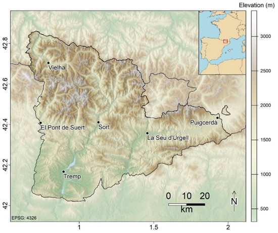
Figure 1.
Study area location with the main population centers.
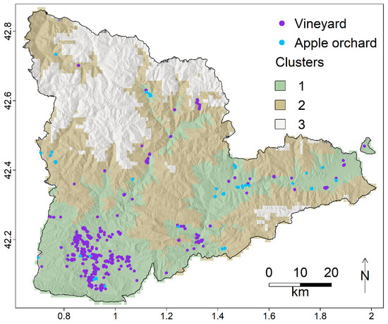
Figure 2.
Cluster map classifying the three different regions according to climate. Dots represent existing plantations (2022) for vineyards (purple) and apple orchards (blue).
Even though in the territory of Catalonia there are 11 appellations of origin, the land object of this study only bears a small portion of Denomination of Origin (DOP) DO Costers de Segre (notably in the Conca de Tremp subregion). Hence it is a new territory to explore, more challenging in terms of yield and commercialization, but also without the constraints imposed by appellations on varieties, yields, which allow the growers to offer a unique product from a novel terroir, which could imply a market advantage. On the apple side, although there is no apple growing tradition in this region, it can offer different products of high quality and a diversification of other products such as juice, jam or cider to explore as new markets.
For the specified region, data was collected and classified into three main categories: climatic data provided by the Catalan Meteorological Service (SMC, acronym in Catalan) at a 1000 × 1000 m regular grid. This was obtained from simulations of regionalization processes performed by statistical techniques (technique of analogs) by the SMC for a control period (1971–2000) and for several forced climate projections until 2050 [48]. Hail episodes were only available as daily probability data from 2013 onward and were directly obtained from the SMC at a 1000 × 1000 m regular grid; soil data obtained from the European Soil Data Centre at various resolutions; and topographic data acquired from the Cartographic and Geological Institute of Catalonia at a 15 × 15 m regular grid. Climatic indicators (except for hail) were calculated using daily maximum and minimum temperatures and accumulated precipitation for the reference climatic period (1991–2020) as defined by the World Meteorological Organization [49]. All indicators were rescaled, when necessary, using zonal statistics (mean) to match the 1000 × 1000 m regular grid from the SMC, which served as the reference template for all raster layers used in the analysis. These operations, along with the suitability analysis, were performed in R Statistical Software (v4.3.1; [50]) through the terra R package (v1.7; [51]).
Using the k-means clustering process [52], all the pixels were classified into 3 groups for an initial exploratory analysis and to allow for better visualization of how climatic variables behave in the study area. Results from the clustering analysis are displayed in Figure 2 and Table 1.

Table 1.
Summarization of annual rainfall and temperatures for each cluster in the reference period (1991–2020). Months are grouped in winter from January to March, spring from April to June, summer from July to September, and Autumn from October to December. T = Temperature; Max. = Maximum; Min. = Minimum.
The following subsections explain each step of the approach (Figure 3).
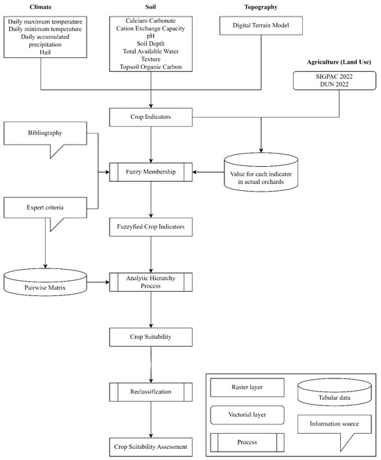
Figure 3.
Flowchart with the general overview of the multi-criteria analysis approach.
2.2. Crop-Specific Suitability Indicators
The indicators included in the multi-criteria analysis were first identified through a review of key articles [12,19,21,28,29,30,31,32,33,34,35,36,37,38,39,40,41,42,43,44,45]. The selection was then made by the expert group (Table 2), based on their relevance in understanding general climate characteristics of vineyards and apple orchards regions, their ability to depict cultivar suitability, and their widespread acceptance and utilization in various regions. In-depth details and explanations regarding each calculated indicator and its description are provided in Table S1 of the Supplementary Material.
Table 2.
Distribution and experience of expert group members.
The complete set of indicators was categorized into three primary groups: (a) climate, (b) soil, and (c) topography.
(a) For climate: the Hydrothermic index of Branas, Bernon, Levadoux (BBL) accounts for the influence of temperature and rainfall on grape production; Cold Days late spring (CDls) represent cold waves; Frost Risk early autumn (FRea) details the frost occurrence during the final stages of maturation and the start of harvest; Frost Risk late spring (FRls) has the same function as FRea but for flowering and the initial stages of fruit formation; Growing Season Precipitation (GSP) summarizes the total precipitation during all the annual development cycle; Growing Season Temperature (GST) measures the average temperature during the same period as GSP; Hail (Ha) represents the days with a high probability of hailstorms during flowering and the initial stages of fruit formation; the Heliothermal Index of Huglin (HI) provides information regarding the level of heliothermal potential and about the sugar potential according to variety; Night Cold Index ripening (NCIr) is a night coolness variable that takes into consideration minimum temperatures during ripening to improve the assessment of qualitative potentials of wine-production regions; Net Hydric Needs (NHN) represents the theoretical amount of water required by crops that is not supplied by rainfall or soil moisture; Stressful Hot Days ripening (SHDr) shows heat waves that can cause burn scars or loss of fruits; the Winkler Index (WI) or Growing Degree Days (GDD) classifies regions based on the heat accumulation during the growing season.
(b) For soil: Calcium Carbonates (CaCO3) address some measure of the soil structure and aggregation, with an excess negatively affecting the mineralization rate of the soil organic matter [53]; Cation Exchange Capacity (CEC) exhibits the soil’s ability to retain cations; pH (pH) gives an indication of the nutrient balance and fertility; Soil Depth (SD) offers an estimation of the potential available volume for roots to expand into, but also indicates the soils’ potential moisture holding ability; Total Available Water (TAW) is the volume of water that is nominally available for plant growth; Texture (Te) shows different soil properties in terms of agricultural use such as the drainage and nutrient retention capacity; Topsoil Organic Carbon (TOC) is measured in the first 40 cm and expresses the soil quality and fertility.
(c) For topography: Aspect (As) affects the angle at which sunlight hits the vineyard and its total heat balance characteristics; Growing season Solar Radiation (GSR) affects the soil and air temperature, transpiration, fruit maturation, soil moisture, and atmospheric humidity during the annual development cycle; Slope (Sl) is important to soil water drainage, but it also affects the daily maintenance of crops in direct relation to machine maneuverability (the maximum acceptable threshold is variable, but a safe value is usually considered to be below 10).
Growing seasons were defined and divided into the most important phenological stages for each crop. For grapevines, bud break–flowering (April–June) and maturation–harvest (August–October) were especially vulnerable to negative weather events (particularly frost) due to their importance to final production [28,54]. For apple orchards, bud break–flowering (April–May) and maturation–harvest (September–October) were also especially vulnerable to negative weather events [23]. The phenological stage of apple bloom precedes that of grapevine flowering, which makes them more susceptible to frost damage and, consequently, to a decrease in final yield. Various studies have corroborated total yield losses caused by late spring frosts (T° < −5 °C) occurring towards the end of May [23].
2.3. Fuzzification
The complexity of the indicators involved in the model and their relationship with each crop implies that suitability thresholds are not abrupt but rather gradual [55]. Therefore, fuzzy logic was employed to enable the integration of numerical and categorical variables across different scales, enhancing the expression of sustainability assessment indicators [56,57].
Fuzzy logic allows the representation of the data distribution according to a user-imposed ‘optimum’ mid-point and spread value for different model/fuzzy membership types, which yields a more realistic output compared to Boolean methods. The spread value defines the width and character of the transition zone and directs the distribution of the data over a range of associations from 0 (not a member) to 1 (definitely a member) [58]. In the model, different proposed membership functions were used to represent distinct ways in which changes in factor values were thought to influence suitability (see Figure S2 from Supplementary Material).
To define the most appropriate value for each individual indicator in relation to crop suitability, a combination of three complementary criteria was utilized. Firstly, expert criteria played a critical role in defining optimal and inadequate thresholds, a method recognized as a valuable source for modeling purposes [56]. This work was made possible through collaboration with a dedicated team of crop specialists, including researchers and technicians. Participants were assembled based on their specific knowledge of each crop (Table 2). All experts involved in the assessment are also co-authors of this manuscript, ensuring that their specialized knowledge was directly integrated into the methodological design and interpretation of the results. Their combined years of experience in vineyards and apple orchards were invaluable to the success of this project. Secondly, a review of journal articles and other published data [34,35,39,41,44,54,59,60,61,62,63,64,65] provided information to compare the values proposed by expert groups. Thirdly, using actual agricultural plots [46,47], the value of each indicator was extracted and summarized to visualize how they behave in an already-cultivated area. The only exception where fuzzy logic wasn’t applied was with SD and Te because of the categorical format of the original data. Those were directly reclassified.
2.4. Analytical Hierarchy Process
To address the complex nature of the problem and integrate all selected indicators within a multi-criteria decision analysis (MCDA), the AHP was employed using datasheets. The AHP is used to derive ratio scales from both discrete and continuous paired comparisons which reflect the relative strength of preferences. In its general form, it is a nonlinear framework for carrying out both deductive and inductive thinking without the use of syllogism by taking several factors into consideration simultaneously, allowing for dependence, feedback, and making numerical tradeoffs to arrive at a synthesis or conclusion [27]. This method allows resolving complex land management problems by identifying the best alternatives, and it is a well-known multi-criteria technique that has been widely incorporated into GIS-based suitability procedures [31,66,67]. It calculates the required weighting factors with the help of a pair-wise matrix where all identified relevant criteria are compared against each other with reproducible preference factors. It then aggregates the weights of the criterion map layers. The pair-wise comparison method employs an underlying semantic scale with values from 1 to 9 (with 9 representing absolute importance and 1 absolute triviality) to rate the relative importance of two elements of the hierarchy [27,68]. This comparison between indicators was performed using the expert criteria proposed by the researchers and technicians, which is crucial to weighing the importance of all the criteria in the model as not all of them are of equal importance [69].
A pair-wise comparison matrix was first constructed only between the three main groups (climate, soil, and topography) to categorize the importance among them. In a second step, each of the indicators was individually compared to the others of the same main group. This provided the relative importance of each indicator inside its group. To obtain the final weight, each indicator’s relative value was multiplied by its main group weight.
The weights taken from the pair-wise matrix were then subjected to the Consistency Ratio (CR). This provided information about the compatibility preferences between all the weights in the form of a resulting number which indicated how far the comparisons are from a consistent matrix. A value of 0.10 or less indicates a reasonable level of consistency [27] but a CR greater than this threshold questions the credibility of judgements of the decision-maker and entails the revision of the pairwise matrix until it achieves a CR lower than the threshold.
2.5. Crop Suitability Assessment
For each pixel and indicator, the value obtained after the fuzzification process was multiplied by the corresponding final weight derived from the AHP. Subsequently, the suitability map for each crop was generated by summing the weighted indicator values for all indicators associated with the same pixel.
To classify the resulting suitability, seven classes were defined from less to more suitable. Although the suitability classification system is inspired by the FAO framework [70,71], it does not include any cost analysis, and it was established to improve the interpretation of the results. Consequently, the system varies in the classes proposed, but it better suits the needs of the analysis and the representation of the results, working on a sliding scale in which criterion values range from 0 (totally unsuitable) to 1 (very highly suitable). Consequently, the interpretation of the classification of each pixel is strongly dependent on criterion. The seven suitability classes in ascending order are: minimal (0–0.3), very low (0.3–0.4), low (0.4–0.5), moderate (0.5–0.6), good (0.6–0.7), very good (0.7–0.8), and high (0.8–1).
3. Results and Discussion
The primary environmental variables (climate, soil, and topography) influencing land suitability for grapevine and apple productivity in mountainous regions were examined for a study area located in the Southern Pyrenees and Pre-Pyrenees. The assessment of crop suitability in this region, where these crops have significantly declined or ceased to be cultivated in recent decades, required a collaborative effort. The selection of indicators and their weighting in the final multi-criteria analysis were crucial in determining the most suitable sites for vineyards and apple orchards. It was essential to correctly define indicators that may potentially limit plant health or yield, such as frosts. If a given indicator has not been utilized previously, it is necessary to develop new ones considering the crop’s phenological cycle and its most vulnerable stages. This task was challenging due to the scarcity of data for the conditions studied, which introduced some uncertainty in defining those indicators and their temporal scale. Additionally, relying on data from existing orchards in mountainous regions could lead to misjudgments, as these may not be located in good production areas [72,73]. Therefore, decisions should be based on a consensus among experts and the observed data. Like other MCDA methods that rely on expert knowledge, the results of this study had a subjective element, reflecting the perceptions of the participating group. To address this, the weights assigned to indicators can be easily adjusted to accommodate diverse perspectives and evolving trends in the climate, cultivation methods, and varietals in future studies.
3.1. Suitability Indicators
The main driving factor for assessing suitability in mountainous areas is the shifting climate conditions related to altitude and exposure due to orography variability. This creates a wide range of climate conditions, complex slopes, and aspects, which play a crucial role in ensuring consistent yields and high quality [74]. The primary impact observed in the climatic indicators for both vineyards and apple orchards was the distinct contrast between the conditions found in valleys compared to those on mountain slopes and peaks, but also between hillsides depending on their aspect. A spatial pattern was visible highlighting the lower zones and sunny hillsides (mildest climate) in contrast to higher zones and shady hillsides (more adverse weather conditions). Figure 4 shows one indicator as an example (FRls) where this pattern is visible, but more cases can be consulted in Figure S1 of the Supplementary Material (CDls, FRea, GDD, GST, HI, SHDr, and WI). In this way, valleys and sunny hillsides were characterized by having generally moderate frost days in the middle of spring (2–5), none or a few frost days in late spring (0–2), and few frost days in early autumn (1–5). Temperatures were more moderate than the rest of the territory (>13 °C), which may also produce stressful hot days (0–10). In addition to an increased probability of experiencing periods of high temperatures, these locations also provided favorable conditions for the development of mildew (Plasmopara viticola) (BBL > 4233). The accumulated precipitation did not represent a limitation (>300 mm), which was also represented in the NHN (generally < 30 mm, except for an area to the south-west that needs between 30–50, 50–100 mm, and at the most extremes sites almost 150 mm). The probability of hailstorms (Figure 4) during flowering did not follow a distinguishable pattern between valley and mountain slopes. Despite covering fewer than 15 pixels in total, the most vulnerable areas could still endure up to 7 hail days. Typically, however, these regions were expected to experience no more than 5 hail days.
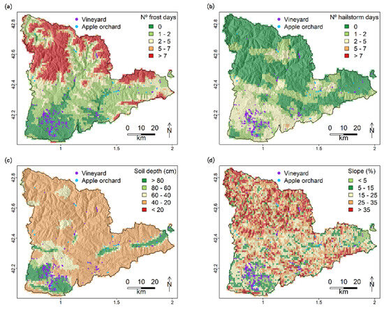
Figure 4.
Spatial distribution of four indicators. (a) FRls (01/05–30/06); (b) Ha; (c) SD; (d) Sl. Valleys and hillsides are especially visible on the FRls map.
The spatial analysis of soil indicators revealed a diverse range of properties that are intricately linked to key soil-forming factors like topography, parent material, and climatic conditions. These indicators varied throughout the territory and were especially unique in the south-west zone where a piggyback foreland basin can be found. Here, a high CaCO3 content hindered good grapevine and apple production (0–4 and 16–45%). The rest of the territory contained a medium-low or medium-high percentage of CaCO3 and there were some valley pixels with an optimum concentration. Similarly, pH resulted in less favorable in the basin but without being as restrictive as carbonates. TOC was lower in part of the basin and tends to also show diminished values in the most extensive and plain valleys. Contrary to those patterns, both SD (Figure 4) and TAW were higher (60–80 cm and 50–>100 mm, respectively) in the basin and on the extensive plains than in the rest of the territory (<40 cm and 20–50 mm). CEC allowed one to differentiate between sub-optimal to optimal zones (15–25 cmol/kg) and its distribution was mostly adequate overall (>15 cmol/kg). Te also created some divergence between pixels from the optimum (Clay-Loam/Loam/Sandy Loam) to the least appropriate (Clay/Silt/Sand) classifications, but those latter classes were rather marginal, and the spatial distribution of this indicator was mostly very adequate.
As and Sl (Figure 4) were fundamental factors for crop cultivation, affecting the amount of solar radiation reaching the soil. Slope increases the hours of daily sunshine but, on the other hand, limits mechanization and increases erosion when it is very steep [32]. The findings demonstrated a clear delineation of areas that were conducive to optimal solar radiation absorption (South/South-east) and those that were less favorable (North). Valleys exhibit marked disparities in orientation due to their predominant north–south alignment, except for the Cerdanya valley (situated eastward within the study region), which is uniquely oriented from east to west, and thereby receives increased solar radiation influx compared to other valleys in the Pyrenees region.
3.2. Fuzzification
One of the criticisms leveled at the conventional land-use suitability analysis is that the underlying assumptions of precise input data are unrealistic. In a complex land-use suitability analysis, it is difficult to provide accurate numerical information required by conventional methods based on Boolean algebra. Fuzzy set theory and logic can address issues related to vagueness, imprecision, and ambiguity in land-use suitability procedures [39]. This becomes especially useful when dealing with problems in which the source of fuzziness is the absence of sharply defined criteria [75].
Through the transformation of each indicators’ raw values using fuzzy membership functions, suitability indicators were obtained. Scores ranged from 0 to 1, e.g., regions with a score of 0 represented the least suitable land for developing each crop and a score of 1 indicates great potential for growth and development in that location. The individual fuzzy membership function for each indicator can be consulted in Figure S2 and the reclassification tables for the categorical ones in Table S2 of the Supplementary Material.
The percentage for each class is reported in Figure 5. Some indicators showed a high suitability for both crops (75%), such as SHDr, pH, NHN, CEC, and TOC. In addition, Te showed a high suitability for vineyards and Ha for apple orchards. On the other hand, there were a few indicators with a more restrictive distribution. Slope, for example, negatively weighted between 50–75% of the territory. A similar pattern can be seen for TAW, GST, BBL, CDls, and GSR. For grapevine, FRls exhibited a more suitability distribution; however, for apple, FRls exhibited very low values overall (70% of the area with less than 0.3). This change was due to the temporal window of the indicator, i.e., it was earlier for apples than grapevines, which involved a higher probability of frost days (Table S1 of the Supplementary Material). SD and TAW, although not having values between 0–0.2, most of them didn’t exceed the 0.5 threshold (occupying these values 85–70% of the whole study area).
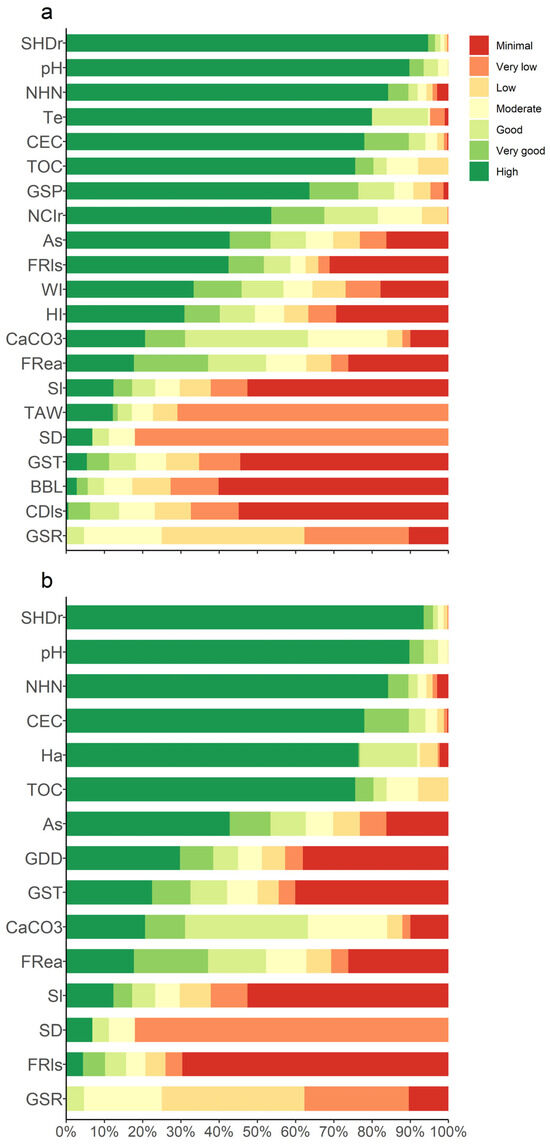
Figure 5.
Suitability classes distribution for each indicator sorted by accumulated percentage of area covered for vineyards (a) and apple orchards (b). The figure uses the acronyms of each of the indicators described in Section 2.2.
3.3. Analytical Hierarchy Process
This procedure greatly reduced the conceptual complexity of the analysis since only two components were considered at every comparison. This allowed for an independent evaluation of the contribution of each criterion, thereby simplifying the decision-making associated with the suitability of vineyards and apple orchards. Although this method is reliant upon the judgment of experts to determine site suitability, errors related to judging the relative importance of factors on site suitability analysis can be both detected and corrected [76]. The resulting pairwise matrixes can be consulted in Table S3 (for vineyards) and Table S4 (for apple orchards) of the Supplementary Material and the weights derived from each pair-wise matrix are summarized in Table 3.
Table 3.
Resulting indicators’ weight for each main group (relative weight) and in the final analysis (final weight) for vineyards (a) and apple orchards (b). The table uses the acronyms of each of the indicators described in Section 2.2.
For vineyards, the comparison between the main groups highlighted the importance of climate (63%) over topography (26%), with soil coming last (11%). Relative weights are rated inside each of the main groups, and a scalation to obtain the final weight for the comparison was needed. This process was achieved by multiplying the main indicator weight to which the indicator belongs by the relative weight of that indicator. If all were considered to have equivalent weights in assessing crop suitability, the value would be around 5%. For climate, NHN (16%) and FRls (15%) were considered the most important indicators to assess environmental suitability. The least weighted were BBL, CD, NCIr, and SHDr, all with values below 3%. The rest of the climate indicators were weighted at around 5%. Soil indicators obtained a very low final weight due to the low main group value (11%), which greatly influences how determinant this group was in the analysis. Only pH was close to 5% and the rest were 2% or less. Topography indicators had values over 5% (GSR 14% and As 9%) and one with a low weight (Sl 3%).
For apple orchards, the comparison between the main groups also showed the importance of climate (69%), achieving a value even higher than that of grapevine. In addition, it decreased the difference between soil (13%) and topography (18%). In this case, equal value for all the components of the analysis would be around 7%. Climate indicators highlighted the effect of Ha (25%) and FRls (24%). FRea, GDD, GST, and SHDr were all below 5%, and NHN was the only indicator close to 7%. Soil values were distributed in two similar groups, with CaCO3, pH, and TOC presenting a very low percentage (1%) and CEC and SD being 5%. Topography had an equal value for both As and GSR (3%) and a higher value for Sl (13%).
Overall, both crops were primarily influenced by climatic conditions; however, vineyards were more responsive to hydric needs, frosts risk during late spring and solar radiation, while apple orchards were more dependent on hailstorm risk, frost risk during late spring and slope.
The Consistency Index was correct for all comparison matrices with values equal to or below 0.10 (Table 4).
Table 4.
Consistency Index for each crop. Main group was composed of climate, soil and topography.
After fuzzification, although many indicators had percentages of more than 75% of the highest class of adequacy (Figure 5; e.g., SHDr, pH, Te, CEC, and TOC), these had a very low weight in the final analysis in percentage terms (Table 3), so that their contribution to the final result was not as significant as others that had a lower proportion of pixels with the highest weighting but a higher value of final weighting (e. g. NHN, FRls, and As). In this way, the best pixels were highlighted when a combination of the highest values of the most weighing indicators converged in a region of space. On the contrary, an accumulation of negative values for high weighting indicators involved low suitability pixels. The main group weighting also had a significant impact on how its indicators performed in the final analysis. In the comparison of the main indicator groups, climate emerged as the dominant factor influencing suitability for both grapevine and apple cultivation, followed by topography and then soil.
3.4. Suitability
Suitability evaluation for vineyards and apple orchards (Figure 6 and Figure 7) resulted in around 1401 (0.2%) and 7704 ha (1.3%) of highly suitable land, respectively. Following this classification, in descending order, very good suitable plots represented around 168,167 (28.6%) and 70,530 (12.0%) ha, respectively; good suitable classes around 176,461 (30.0%) and 141,052 (24.0%) ha, respectively; moderate around 93,922 (16.0%) and 258,360 (43.9%) ha, respectively; low around 133,620 (22.7%) and 106,425 (18.1%) ha, respectively; very low around 14,402 (2.4%) and 3902 (0.6%) ha, respectively; and minimal was not defined in any pixel over the whole area.
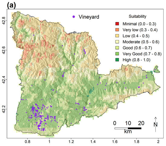
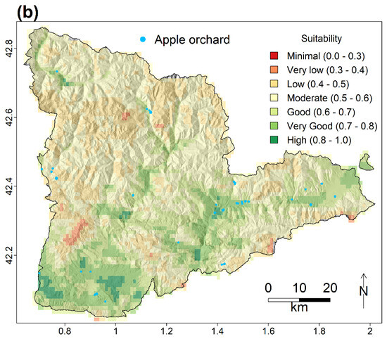
Figure 6.
Suitability maps for vineyards (a) and apple orchards (b) as obtained by the weighed combination of rasters for each indicator and crop.
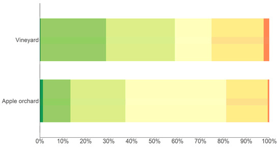
Figure 7.
Bar plot summarizing the cumulative area covered for each suitability class from Figure 6 in percentage of covered area for each crop.
The results underscored the significant influence of shifting climate conditions, which are intricately linked to variations in elevation and exposure due to orographic features. These factors generate diverse climate conditions, complex slopes, and exposure patterns that profoundly impact sustained yields and crop quality [74]. This is one of the most crucial aspects to consider when promoting Land Use Changes (LUC) in mountainous areas, as some authors identified steep and terraced slopes, wet areas without drainage, and areas isolated from roads and settlements as being the most vulnerable to land abandonment [77]. While this last issue and other social or biodiversity aspects were considered crucial, they do not affect site suitability as is the crop biophysical interaction with the climate, soil, and terrain. For this reason, they were not included in this suitability model.
Suitable areas were generally concentrated in the lower basins and on sunny hillsides where warmer climate conditions, solar exposure, and gentle slopes may support grapevine and apple cultivation without requiring impractical effort—both economically and environmentally (Figure 8).
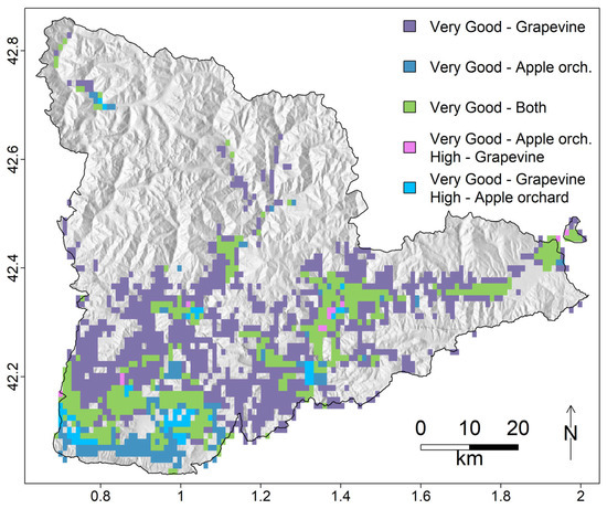
Figure 8.
Combined suitability map selecting only pixels were values were at least “Very Good”. Different blends are displayed, except for the combination of “High” for both crops, which was not existent.
According to the different indicators adopted in this study, for vineyards, areas with lower hydric needs, lower late spring frost risk, higher incident solar radiation, and a favorable aspect (mainly south) are the most suitable. For apple orchards, areas with low hail probability and lower late spring frost risk, smoother slopes, and lower hydric needs were the most suitable. In general, the relationship between frost days in spring and production was shown to be one of the most influential indicators for both crops in terms of assessing suitability due to its huge impact on annual production. Through personal interviews with farmers, it was confirmed that this meteorological phenomenon had the most significant impact on their crops. Some studies also recorded full-production losses and flower injuries caused by spring frosts [23] and other extremely low temperatures events [25,78]. In some areas with adequate water requirements and temperatures, excessive steepness could represent a significant barrier for production caused by the limited mechanization possibilities [32], which may be overcome by terracing the terrain (thus increasing implementation costs). On the contrary, positive effects were attributed to slope, mainly with south (and west) facing aspects, resulting in an increased incidence of solar radiation. Selecting landsites with high exposure to solar radiation may be crucial in mountainous areas in the Northern hemisphere where we expect to have low Winkler index values. This, therefore, highlights the role of temperature in the attainment of acceptable production levels. NHN is another important indicator because it quantifies plant water demands based on evapotranspiration and soil water holding capacity [7]. Mountainous regions do not typically have irrigation systems in place, as historically, extensive cattle farming or agriculture practices in these areas did not require additional water inputs. Consequently, numerous locations within our study zone lack access to an irrigation infrastructure. This may be the most significant limiting factor to future plantations, especially for apple orchards. Vines may remain rainfed shortly after their establishment, but apple trees are highly dependent on water input to achieve a minimum level of production in intensive orchards, but apple trees are highly dependent on water input to achieve a minimum level of production in intensive orchards.
Despite the barriers to successfully developing a productive activity for grapevines and apples, other factors highlight the benefits of doing so. Both will be affected by climate change conditions in their habitual production areas, because of increased temperatures and droughts [2]. Various studies analyzed altitude as an adaptation strategy resulting in favorable outcomes for vineyards [20]. In the case of apple orchards, lower temperatures during summer are favorable for better fruit coloration. Additionally, improvements in organoleptic quality, in particular, firmness, texture, juiciness, and flesh chewiness and crunchiness, have also been reported [23].
Another argument for inducing LUC is related to reverting land abandonment through recultivation and promoting better fire-resistant mosaics in highly flammable landscapes [79]. High Nature Value farmlands (HNVf; as described by Beaufoy, et al. [80]) in mountainous rural landscapes compose low-intensity agricultural and livestock activities, which are often associated with areas rich in biodiversity. Lecina-Diaz et al. [81] results suggest that the potential net suppression cost savings can be substantial under HNVf scenarios. Previous studies also concluded that the promotion of agriculture increases protection against burned areas in agricultural and forest land cover. Moreover, promoting agriculture can help suppress wildfires to the detriment of more flammable landscapes [79,82]. An efficient scenario combines both HNVf with fire-smart management (defined as “an integrated approach primarily based on fuel treatments through which the socio-economic impacts of fire are minimized while its ecological benefits are maximized” by Hirsch et al. [83]). However, as mentioned earlier, agriculture practices in mountainous regions may be uncompetitive and difficult for local people to perform due to the demanding conditions in comparison to habitual cultivation areas. In addition, farmers are only financially rewarded for their production, but not for the societal benefits derived from the provision of good public ecosystem services and their contribution to wildfires suppression and/or to landscape maintenance. The complex interactions between crops and climate, fire-vegetation dynamics, and LUC under climate change hinder the efficient management of rural landscapes [84,85]. Therefore, agricultural land management in mountainous areas should consider multiple objectives and needs. In addition, any decision regarding crop potential should be based on marketable production and sustainable management strategies to guarantee maintained production and provide long-term economic benefits.
Several studies have assessed land suitability from different perspectives [28,29,30,31,32,33,34,35,36,37,38,39,40,41,42,43]; however, very few have focused on mountainous regions, and none have incorporated highly influential features such as FRls or FRea (see Table S1 of Supplementary Material) or combined methodologies within their approach. In this study, we developed a suitability assessment approach designed to integrate diverse variables across multiple scales. The relationship between each indicator and cultivation suitability was established using gradual, continuous functions (fuzzy membership functions) specifically defined for each variable. This procedure allowed us to represent nonlinear responses and thresholds, avoiding abrupt transitions inherent in Boolean classifications. By doing so, it captures the inherent complexity and variability of the indicators included [55]. Furthermore, it enhances the sensitivity and explanatory power of indicators, enabling more realistic evaluations of suitability [56,57]. The posterior use of AHP proved to be an appropriate and efficient choice, as it enabled a structured quantification of expert knowledge and facilitated the comparison of heterogeneous variables influencing crop suitability. Altogether, the approach is easily adjustable to different agro-climatic and socio-economic contexts if used hand in hand with the knowledge of sector experts and farmers. Its structure and input can also be readily modified to reflect local suitability conditions. For these reasons, we consider it applicable to climate change scenarios and the exploration of new cultivable areas. The suitability assessment approach (Figure 3) relied on a multi-criteria analysis that included the following: (i) gathering data and the determination of a spatial resolution to work with; (ii) the selection of the most relevant indicators to assess crop suitability derived from the data; (iii) the definition of fuzzy membership functions for each indicator; (iv) the weighting of the main groups and indicators inside each of the main groups; and (v) the overlaying of all the layers to obtain a final suitability map. This approach to crop suitability modeling enables a more valuable and informative grading of land suitability than those derived from a Boolean approach.
3.5. Validation
Although values for each indicator in existing vineyards and apple orchards were extracted for a better understanding of their behavior in the current context, the location of these plantations were not directly used to evaluate the overall performance of the land assessment system. This decision was based on the consideration that existing orchards may not necessarily be located on the most suitable plots. In mountainous regions, farmers willing to establish vineyards or apple orchards are often constrained by socio-economic conditions and lack the opportunity to survey and select highly climatically optimal sites. Similar observations have been reported by other authors when assessing crop suitability using modeling approaches [18,72,73]. In our case, this limitation was even more pronounced given the novelty of these crops in mountainous regions (most farmers commenced this activity less than 15 years ago and, in many cases, these crops do not represent primary economic activity). In addition, surveys conducted among farmers showed that landowners typically planted directly on their property without conducting detailed suitability analyses, while tenants established crops wherever available, and affordable plots could be found.
These contextual factors strongly influenced the selection of the suitability assessment approach used in this study, over other data-driven multi-criteria analysis like machine-learning algorithms. MaxEnt [86], for example, is a widely used model. Moreover, it has been applied to crop suitability area delimitation [70,87] and specifically for vineyards [44] and apple [45]. Although its demonstrated applicability in assessing suitability, in the specific case of mountainous regions, the scarcity of representative and robust datasets will usually not provide a good baseline for applying machine-learning methods. Consequently, the fuzzy membership method combined with the AHP was considered the most appropriate method for this study, offering both methodological consistency and practical adaptability to the specific conditions of mountainous agricultural systems.
3.6. Constrains
This study employed a robust and valid approach to identify potential locations for grapevine and apple cultivation in mountainous areas. However, some challenges and limitations were encountered during the process. One significant constraint was the scarcity of data on long-standing plots where these crops are cultivated. As a relatively new activity in mountainous areas, it was difficult to determine how indicators should behave to assess the best productive conditions. Given the relatively new activity in mountainous regions, determining the behavior of indicators to assess optimal growing conditions proved challenging. Relying on expert knowledge was crucial to overcome this limitation. Access to a high-productivity dataset could enable the use of quantitative models to predict productivity across the distribution range of these crops [70].
The high number of indicators used to perform the model was another challenge faced during data analysis. Constructing the pair-wise matrix for indicators within the main groups proved cumbersome given the large number of comparisons required while maintaining consistency. As a result, a higher CI was usually obtained when checking relations in more dense main groups (Table 4). The objective was to identify how each indicator’s values were spatially distributed in the study area, allowing for the individual identification of behavior in each pixel. With this approach, when selecting specific plots inside a pixel, it is possible to assess how many days it is expected to freeze in late spring or the net hydric needs. To mitigate complexity, Principal Component Analysis (PCA) could be employed before conducting the fuzzification process, similar to other multi-criteria analysis for crop suitability [40,87].
Lastly, the study utilized a 1000 × 1000 m regular grid for calculating indicators and suitability, primarily due to the limitations in downscaling. While climatic variables were directly provided at this resolution, effective downscaling techniques exist to obtain high-resolution datasets [88,89]. Performing a full climatic data downscaling to harmonize spatial resolution into a finer resolution (e.g., 100 × 100 m), however, would have been complex, especially for precipitation. Consequently, topography variables that were originally obtained at a high resolution (15 × 15 m regular grid), were rescaled to match the base study grid. Soil data was obtained at different resolutions, but it was all rescaled to 1000 × 1000 m as no downscaling technique was found to satisfactorily perform the process for all the indicators without leading to errors, due to a dependency on on-site characteristics. Some studies did work with downscaling methods for variables like soil moisture [90], but none was found for all the indicators included in our analysis. Consequently, some uncertainty is associated with the environmental parameter classification in each pixel due to the spatial variation not being captured in the databases. Settou et al. [91] provided insights into how the database raster resolution may affect the final suitability area delimitation in MCDA. For this reason, when planning orchards with a suitability analysis, a local soil and topography analysis is needed to confirm adequate zones both for plant development and labor constraints.
3.7. Perspectives
Mosaic landscapes created by HNVf solutions, such as newly implemented vineyards or apple orchards, may promote resistance to Extreme Wildfire Events (EWE). An ongoing analysis is overlapping highly suitable areas with firefighting priority zones to identify plots susceptible to LUC towards the woody crops analyzed in this study. The aim is to select plots that are located within priority areas and are conducive to transitioning into vineyards and apple orchards. During this selection process, factors such as the plot size, accessibility, and irrigation potential are also considered. However, to mitigate wildfire impacts on ecosystem services, integrated solutions must address key drivers in an economic, social, and environmental manner [92]. Economic and social aspects were not considered in this specific part of the study, as they were not the objective when developing the approach. Nevertheless, these factors are crucial, and identifying key economic constraints and public perspectives on this novel activity is necessary for the successful implementation of the proposed approach. In parallel with the overlap analysis, active work is identifying socio-economic limitations affecting mountainous regions, mainly through personal interviews with farmers involved in vineyards or apple orchards in those regions.
In our study, we successfully performed a suitability assessment for the selected reference climatic period (1991–2020). To further understand how the distribution of vineyards and apple orchards may shift under different future climate scenarios, this same approach could be applied to identify projected suitable areas. Such a forward analysis could help identify land with maximum suitability for various climate change scenarios, providing a valuable tool for stakeholders in determining planting locations.
In the future, it will also be crucial to account for the projected temperature increase in mountainous regions compared to lower geographical areas, as was described in the Third Report on Climate change in Catalonia [93]. The combined effects of rising temperatures and more frequent heat waves could produce synergistic negative impacts on crops’ viability, emphasizing the need for continuous adaptation and monitoring efforts.
4. Conclusions
In conclusion, the suitability assessment for vineyard and apple orchard cultivation in mountainous regions revealed the intricate interplay of climatic, soil, and topographic factors. Shifting climate conditions, characterized by elevation and exposure variations, significantly influenced crop suitability. Lower basins and sunny hillsides generally exhibited highest suitability, largely due to their reduced incidence of late spring frosts, which was considered one of the critical limiting factors for both crops. Given that circumstance, implementing frost protection measures should be considered essential for ensuring stable yields and minimizing production losses.
The application of fuzzy membership functions combined with the AHP facilitated the integration of suitability indicators, effectively identifying areas with high potential for crop development and highlighting factors affecting. The predominance of climate as in determining suitability underscored the importance of considering restrictive climatic indicators, such as frost risk and hail, in agricultural planning.
Overall, the results provide valuable insights for stakeholders involved in agricultural decision-making by offering a comprehensive understanding of the spatial variability in suitability factors. By integrating these findings into land management strategies, policymakers and farmers can optimize crop production practices, enhance resilience to environmental challenges and resistance to EWE, and promote sustainable agriculture in mountainous regions.
Supplementary Materials
The following supporting information can be downloaded at: https://www.mdpi.com/article/10.3390/land14112135/s1, Table S1: Summary of indicators; Table S2: Reclassification tables for each categorical indicator; Table S3: Pairwise matrices for vineyards; Table S4: Pairwise matrices; Figure S1: Spatial distribution of indicators; Figure S2: Fuzzy membership function for each indicator.
Author Contributions
Conceptualization: A.C.-T., F.d.H., M.P., J.L., E.S.-C., R.S. and I.F. Data curation: A.C.-T. and E.S.-C. Formal analysis: A.C.-T. Funding acquisition: F.d.H. and R.S. Investigation: A.C.-T., F.d.H., M.P., J.L., A.S.-O. and I.F. Methodology: A.C.-T. and I.F. Project administration: F.d.H. and I.F. Supervision: F.d.H., M.P., J.L. and I.F. Validation: F.d.H., R.S. and I.F. Visualization: A.C.-T. Writing—original draft: A.C.-T. Writing—review & editing: A.C.-T., F.d.H., R.S., M.P., J.L., A.S.-O., E.S.-C., A.B. and I.F. All authors have read and agreed to the published version of the manuscript.
Funding
The research leading to these results received funding from FIRE-RES Horizon 2020 project under Grant Agreement No. 101037419.
Data Availability Statement
The datasets generated during the current study are available in the FIRE-RES Zenodo repository, https://zenodo.org/communities/fire_res/ (accessed on 12 September 2025) (Casadó-Tortosa, A., de Herralde, F., Savé, R., Peris, M., Lordan, J., Sánchez-Ortiz, A., Sánchez-Costa, E., Barbeta, A., & Funes, I. (2024). Vineyard and Apple Orchard Suitability Maps for Mountainous Areas (Southern Pyrenees and Pre-Pyrenees) (Version v1) [Data set]. Zenodo. https://doi.org/10.5281/zenodo.12621989).
Acknowledgments
This project received funding from the European Union’s Horizon 2020 Research and Innovation Programme under grant agreement No. 101037419—FIRE-RES. We would like to thank the Catalan Meteorological Service for providing climatic data. We would also like to extend our sincere gratitude to all the farmers that participated in the FIRE-RES project and helped us to assess the best conditions to develop a vineyard or an apple orchard in mountainous regions.
Conflicts of Interest
The authors declare no competing interests.
Abbreviations
The following abbreviations are used in this manuscript:
| AHP | Analytic Hierarchy Process |
| As | Aspect |
| BBL | Hydrothermic index of Branas, Brenon, Levandoux |
| CaCO3 | Calcium Carbonates |
| CDls | Cold Days late spring |
| CEC | Cation Exchange Capacity |
| CR | Consistency Ratio |
| EWE | Extreme Wildfire Events |
| FAO | Food and Agriculture Organization |
| FRea | Frost Risk early autumn |
| FRls | Frost Risk late spring |
| GDD | Growing Degree Days |
| GIS | Geographical Information System |
| GSP | Growing Season Precipitation |
| GSR | Growing season Solar Radiation |
| GST | Growing Season Temperature |
| Ha | Hail |
| HI | Heliothermal Index of Huglin |
| HNVf | High Nature Value farmlands |
| IPCC | Intergovernmental Panel on Climate Change |
| LUC | Land Use Changes |
| MCDA | Multi-Criteria Decision Analysis |
| NCIr | Night Cold Index ripening |
| NHN | Net Hydric Needs |
| PCA | Principal Component Analysis |
| SD | Soil Depth |
| SHDr | Stressful Hot Days ripening |
| Sl | Slope |
| SMC | Catalan Meteorological Service |
| TAW | Total Available Water |
| Te | Texture |
| TOC | Topsoil Organic Carbon |
References
- Arias, P.A.; Bellouin, N.; Coppola, E.R.G.J.; Krinner, G.; Marotzke, J.; Naik, V.; Palmer, M.D.; Plattner, G.-K.; Rogelj, J.; Rojas, M.; et al. Technical Summary. In Climate Change 2021: The Physical Science Basis. Contribution of Working Group I to the Sixth Assessment Report of the Intergovernmental Panel on Climate Change; Cambridge University Press: Cambridge, UK; New York, NY, USA, 2021; pp. 33–144. [Google Scholar]
- Blanco-Ward, D.; Monteiro, A.; Lopes, M.; Borrego, C.; Silveira, C.; Viceto, C.; Rocha, A.; Ribeiro, A.; Andrade, J.; Feliciano, M.; et al. Analysis of climate change indices in relation to wine production: A case study in the Douro region (Portugal). BIO Web Conf. 2017, 9, 01011. [Google Scholar] [CrossRef]
- Schultz, H.; Hofmann, M. The ups and downs of environmental impact on grapevines. In Grapevine in a Changing Environment. In Grapevine in a Changing Environment: A Molecular and Ecophysiological Perspective; Gerós, H.M.M.C., Gil, H.M., Delrot, S., Eds.; Wiley: Hoboken, NJ, USA, 2016. [Google Scholar]
- MedECC. Climate and Environmental Change in the Mediterranean Basin—Current Situation and Risks for the Future. In First Mediterranean Assessment Report; Cramer, W., Guiot, J., Marini, K., Eds.; Union for the Mediterranean, Plan Bleu, UNEP/MAP: Marseille, France, 2020; Volume 632, ISBN 978-2-9577416-0-1. [Google Scholar] [CrossRef]
- Funes, I.; Aranda, X.; Biel, C.; Carbó, J.; Camps, F.; Molina, A.J.; Herralde, F.d.; Grau, B.; Savé, R. Future climate change impacts on apple flowering date in a Mediterranean subbasin. Agric. Water Manag. 2016, 164, 19–27. [Google Scholar] [CrossRef]
- Savé, R.; de Herralde, F.; Aranda, X.; Pla, E.; Pascual, D.; Funes, I.; Biel, C. Potential changes in irrigation requirements and phenology of maize, apple trees and alfalfa under global change conditions in Fluvià watershed during XXIst century: Results from a modeling approximation to watershed-level water balance. Agric. Water Manag. 2012, 114, 78–87. [Google Scholar] [CrossRef]
- Funes, I.; Savé, R.; de Herralde, F.; Biel, C.; Pla, E.; Pascual, D.; Zabalza, J.; Cantos, G.; Borràs, G.; Vayreda, J.; et al. Modeling impacts of climate change on the water needs and growing cycle of crops in three Mediterranean basins. Agric. Water Manag. 2021, 249, 106797. [Google Scholar] [CrossRef]
- Vicente-Serrano, S.M.; Zabalza-Martínez, J.; Borràs, G.; López-Moreno, J.I.; Pla, E.; Pascual, D.; Savé, R.; Biel, C.; Funes, I.; Azorin-Molina, C.; et al. Extreme hydrological events and the influence of reservoirs in a highly regulated river basin of northeastern Spain. J. Hydrol. Reg. Stud. 2017, 12, 13–32. [Google Scholar] [CrossRef]
- Montsant, A.; Baena, O.; Bernárdez, L.; Puig, J. Modelling the impacts of climate change on potential cultivation area and water deficit in five Mediterranean crops. Span. J. Agric. Res. 2021, 19, e0301. [Google Scholar] [CrossRef]
- Zhao, G.; Webber, H.; Hoffmann, H.; Wolf, J.; Siebert, S.; Ewert, F. The implication of irrigation in climate change impact assessment: A European-wide study. Glob. Change Biol. 2015, 21, 4031–4048. [Google Scholar] [CrossRef]
- Connor, J.D.; Schwabe, K.; King, D.; Knapp, K. Irrigated agriculture and climate change: The influence of water supply variability and salinity on adaptation. Ecol. Econ. 2012, 77, 149–157. [Google Scholar] [CrossRef]
- Lorenzo, M.N.; Ramos, A.M.; Brands, S. Present and future climate conditions for winegrowing in Spain. Reg. Environ. Change 2015, 16, 617–627. [Google Scholar] [CrossRef]
- Xyrafis, E.G.; Fraga, H.; Nakas, C.T.; Koundouras, S. A study on the effects of climate change on viticulture on Santorini Island. OENO One 2022, 56, 259–273. [Google Scholar] [CrossRef]
- Bernardo, S.; Dinis, L.-T.; Machado, N.; Moutinho-Pereira, J. Grapevine abiotic stress assessment and search for sustainable adaptation strategies in Mediterranean-like climates. A review. Agron. Sustain. Dev. 2018, 38, 66. [Google Scholar] [CrossRef]
- Ahmadi, H.; Ghalhari, G.F.; Baaghideh, M. Impacts of climate change on apple tree cultivation areas in Iran. Clim. Change 2018, 153, 91–103. [Google Scholar] [CrossRef]
- Li, M.; Guo, J.; He, J.; Xu, C.; Li, J.; Mi, C.; Tao, S. Possible impact of climate change on apple yield in Northwest China. Theor. Appl. Climatol. 2019, 139, 191–203. [Google Scholar] [CrossRef]
- Pfleiderer, P.; Menke, I.; Schleussner, C.-F. Increasing risks of apple tree frost damage under climate change. Clim. Change 2019, 157, 515–525. [Google Scholar] [CrossRef]
- Mosedale, J.R.; Abernethy, K.E.; Smart, R.E.; Wilson, R.J.; Maclean, I.M. Climate change impacts and adaptive strategies: Lessons from the grapevine. Glob. Change Biol. 2016, 22, 3814–3828. [Google Scholar] [CrossRef]
- Blanco-Ward, D.; Ribeiro, A.; Barreales, D.; Castro, J.; Verdial, J.; Feliciano, M.; Viceto, C.; Rocha, A.; Carlos, C.; Silveira, C.; et al. Climate change potential effects on grapevine bioclimatic indices: A case study for the Portuguese demarcated Douro Region (Portugal). BIO Web Conf. 2019, 12, 01013. [Google Scholar] [CrossRef]
- Arias, L.A.; Berli, F.; Fontana, A.; Bottini, R.; Piccoli, P. Climate Change Effects on Grapevine Physiology and Biochemistry: Benefits and Challenges of High Altitude as an Adaptation Strategy. Front. Plant Sci. 2022, 13, 835425. [Google Scholar] [CrossRef]
- Modina, D.; Cola, G.; Bianchi, D.; Bolognini, M.; Mancini, S.; Foianini, I.; Cappelletti, A.; Failla, O.; Brancadoro, L. Alpine Viticulture and Climate Change: Environmental Resources and Limitations for Grapevine Ripening in Valtellina, Italy. Plants 2023, 12, 2068. [Google Scholar] [CrossRef]
- Sahu, N.; Saini, A.; Behera, S.K.; Sayama, T.; Sahu, L.; Nguyen, V.T.; Takara, K. Why apple orchards are shifting to the higher altitudes of the Himalayas? PLoS ONE 2020, 15, e0235041. [Google Scholar] [CrossRef]
- Iglesias, I.; Garanto, X.; Farré, X.; Mas, N.; Echeverría, G.; Vila, A.; Segura, F.; Lordan, J. La Poma de Muntanya; Departament d’Agricultura, Ramaderia, Pesca i Alimentació. 2020. Available online: http://agricultura.gencat.cat/ (accessed on 24 January 2024).
- Campos, C.G.C.; Malinovski, L.I.; Marengo, J.A.; Oliveira, L.V.; Vieira, H.J.; Silva, A.L. The impact of climate projections when analyzing the risk of frost to viticulture in the southern region of Brazil. Acta Hortic. 2017, 1188, 165–172. [Google Scholar] [CrossRef]
- Dami, I.E.; Ennahli, S.; Zhang, Y. Assessment of Winter Injury in Grape Cultivars and Pruning Strategies Following a Freezing Stress Event. Am. J. Enol. Vitic. 2012, 63, 106–111. [Google Scholar] [CrossRef]
- Zadeh, L. Fuzzy Logic. Computer 1988, 21, 83–93. [Google Scholar] [CrossRef]
- Saaty, R.W. The Analytic Hierarchy Process—What it is and how it is used. Math. Model. 1987, 9, 161–176. [Google Scholar] [CrossRef]
- Anastasiou, E.; Xanthopoulos, G.; Templalexis, C.; Lentzou, D.; Panitsas, F.; Mesimeri, A.; Karagianni, E.; Biniari, A.; Fountas, S. Climatic indices as markers of table-grapes postharvest quality: A prediction exercise. Smart Agric. Technol. 2022, 2, 100059. [Google Scholar] [CrossRef]
- Honorio, F.; García-Martín, A.; Moral, F.J.; Paniagua, L.L.; Rebollo, F.J. Spanish vineyard classification according to bioclimatic indexes. Aust. J. Grape Wine Res. 2018, 24, 335–344. [Google Scholar] [CrossRef]
- Jones, G.; Duff, A.; Hall, A.; Myers, J. Spatial Analysis of Climate in Winegrape Growing Regions in the Western United States. Am. J. Enol. Vitic. 2010, 61, 313–326. [Google Scholar] [CrossRef]
- Alsafadi, K.; Mohammed, S.; Habib, H.; Kiwan, S.; Hennawi, S.; Sharaf, M. An integration of bioclimatic, soil, and topographic indicators for viticulture suitability using multi-criteria evaluation: A case study in the Western slopes of Jabal Al Arab—Syria. Geocarto Int. 2020, 35, 1466–1488. [Google Scholar] [CrossRef]
- Stanchi, S.; Godone, D.; Belmonte, S.; Freppaz, M.; Galliani, C.; Zanini, E. Land suitability map for mountain viticulture: A case study in Aosta Valley (NW Italy). J. Maps 2013, 9, 367–372. [Google Scholar] [CrossRef]
- Alganci, U.; Kuru, G.N.; Yay Algan, I.; Sertel, E. Vineyard site suitability analysis by use of multicriteria approach applied on geo-spatial data. Geocarto Int. 2018, 34, 1286–1299. [Google Scholar] [CrossRef]
- Chozom, K.; Nimasow, G. GIS- and AHP-based land suitability analysis of Malus domestica Borkh. (apple) in West Kameng district of Arunachal Pradesh, India. Appl. Geomat. 2021, 13, 349–360. [Google Scholar] [CrossRef]
- Beyene, G.; Dechassa, N.; Regasa, A.; Wogi, L. Land Suitability Assessment for Apple (Malus domestica) Production in Sentele Watershed in Hadiya Zone, Southern Ethiopia. Appl. Environ. Soil Sci. 2022, 2022, 4436417. [Google Scholar] [CrossRef]
- Manandhar, S.; Pandey, V.P.; Kazama, F. Assessing suitability of apple cultivation under climate change in mountainous regions of western Nepal. Reg. Environ. Change 2013, 14, 743–756. [Google Scholar] [CrossRef]
- Sánchez, Y.; Martínez-Graña, A.M.; Santos-Francés, F.; Yenes, M. Index for the calculation of future wine areas according to climate change application to the protected designation of origin “Sierra de Salamanca” (Spain). Ecol. Indic. 2019, 107, 105646. [Google Scholar] [CrossRef]
- Vujadinović Mandić, M.; Vuković Vimić, A.; Fotirić Akšić, M.; Meland, M. Climate Potential for Apple Growing in Norway—Part 2: Assessment of Suitability of Heat Conditions under Future Climate Change. Atmosphere 2023, 14, 937. [Google Scholar] [CrossRef]
- Badr, G.; Hoogenboom, G.; Moyer, M.; Keller, M.; Rupp, R.; Davenport, J. Spatial suitability assessment for vineyard site selection based on fuzzy logic. Precis. Agric. 2018, 19, 1027–1048. [Google Scholar] [CrossRef]
- Salata, S.; Ozkavaf-Senalp, S.; Velibeyoğlu, K.; Elburz, Z. Land Suitability Analysis for Vineyard Cultivation in the Izmir Metropolitan Area. Land 2022, 11, 416. [Google Scholar] [CrossRef]
- Lone, F.A.; Ganaie, M.I.; Ganaie, S.A.; Bhat, M.S.; Rather, J.A. Evaluation Criteria for the Suitability of Apple Cultivation in Kashmir Valley, India. Asian J. Agric. Dev. 2023, 20, 71–85. [Google Scholar] [CrossRef]
- Nisar Ahamed, T.R.; Gopal Rao, K.; Murthy, J.S.R. GIS-based fuzzy membership model for crop-land suitability analysis. Agric. Syst. 2000, 63, 75–95. [Google Scholar] [CrossRef]
- Vetharaniam, I.; Müller, K.; Stanley, C.J.; van den Dijssel, C.; Timar, L.; Clothier, B. Modelling Continuous Location Suitability Scores and Spatial Footprint of Apple and Kiwifruit in New Zealand. Land 2022, 11, 1528. [Google Scholar] [CrossRef]
- del Río, S.; Álvarez-Esteban, R.; Alonso-Redondo, R.; Hidalgo, C.; Penas, Á. A new integrated methodology for characterizing and assessing suitable areas for viticulture: A case study in Northwest Spain. Eur. J. Agron. 2021, 131, 126391. [Google Scholar] [CrossRef]
- Xu, W.; Miao, Y.; Zhu, S.; Cheng, J.; Jin, J. Modelling the Geographical Distribution Pattern Of Apple Trees on the Loess Plateau, China. Agriculture 2023, 13, 291. [Google Scholar] [CrossRef]
- Ministerio de Agricultura, Pesca y Alimentación (MAPA). Sistema de Información Geográfica de Parcelas Agrícolas (SIGPAC). 2022. Available online: https://www.mapa.gob.es/en/agricultura/temas/sistema-de-informacion-geografica-de-parcelas-agricolas-sigpac-/visor-sigpac (accessed on 6 April 2023).
- Departament d’Agricultura, Ramaderia, Pesca i Alimentació (DARPA). Mapa de Cultius Declaració Agrària (DUN-SIGPAC). 2022. Available online: https://agricultura.gencat.cat/ca/ambits/desenvolupament-rural/sigpac/mapa-cultius/ (accessed on 6 April 2023).
- Altava-Ortiz, V.; Barrera-Escoda, A. Escenaris Climàtics Regionalitzats a Catalunya (ESCAT-2020). In Projeccions Estadístiques Regionalitzades a 1 km de Resolució Espacial (1971–2050); Servei Meteorològic de Catalunya, Departament de Territori i Sostenibilitat, Generalitat de Catalunya: Barcelona, Catalonia, Spain, 2020; p. 169. [Google Scholar]
- WMO. WMO Guidelines on the Calculation of Climate Normals. 2017. Available online: https://library.wmo.int/viewer/55797?medianame=1203_en_#page=12&viewer=picture&o=bookmark&n=0&q= (accessed on 28 June 2023).
- R Core Team. R: A Language and Environment for Statistical Computing; R Foundation for Statistical Computing: Vienna, Austria, 2023; Available online: https://www.R-project.org/ (accessed on 3 June 2023).
- Hijmans, R. terra: Spatial Data Analysis. 2023. Available online: https://rspatial.org/ (accessed on 3 June 2023).
- Hartigan, J.; Wong, M. Algorithm AS 136: A K-Means Clustering Algorithm. J. R. Stat. Society. Ser. C (Appl. Stat.) 1979, 28, 100–108. [Google Scholar] [CrossRef]
- Virto, I.; Antón, R.; Apesteguía, M.; Plante, A. Role of Carbonates in the Physical Stabilization of Soil Organic Matter in Agricultural Mediterranean Soils. In Soil Management and Climate Change; Academic Press: Cambridge, MA, USA, 2018; pp. 121–136. [Google Scholar] [CrossRef]
- Tonietto, J.; Carbonneau, A. A multicriteria climatic classification system for grape-growing regions worldwide. Agric. For. Meteorol. 2004, 124, 81–97. [Google Scholar] [CrossRef]
- Cornelissen, A.; van den Berg, J.; Koops, W.; Grossman, M.; Udo, H. Assessment of the contribution of sustainability indicators to sustainable development: A novel approach using fuzzy set theory. Agric. Ecosyst. Environ. 2001, 86, 173–185. [Google Scholar] [CrossRef]
- de Vos, M.G.; Janssen, P.H.M.; Kok, M.T.J.; Frantzi, S.; Dellas, E.; Pattberg, P.; Petersen, A.C.; Biermann, F. Formalizing knowledge on international environmental regimes: A first step towards integrating political science in integrated assessments of global environmental change. Environ. Model. Softw. 2013, 44, 101–112. [Google Scholar] [CrossRef]
- Prato, T. A fuzzy logic approach for evaluating ecosystem sustainability. Ecol. Model. 2005, 187, 361–368. [Google Scholar] [CrossRef]
- Malczewski, J. GIS-based land-use suitability analysis: A critical overview. Prog. Plan. 2004, 62, 3–65. [Google Scholar] [CrossRef]
- Jones, G.V.; White, M.A.; Cooper, O.R.; Storchmann, K. Climate Change and Global Wine Quality. Clim. Change 2005, 73, 319–343. [Google Scholar] [CrossRef]
- Cardell, M.F.; Amengual, A.; Romero, R. Future effects of climate change on the suitability of wine grape production across Europe. Reg. Environ. Change 2019, 19, 2299–2310. [Google Scholar] [CrossRef]
- Fraga, H.; Malheiro, A.C.; Moutinho-Pereira, J.; Cardoso, R.M.; Soares, P.M.; Cancela, J.J.; Pinto, J.G.; Santos, J.A. Integrated analysis of climate, soil, topography and vegetative growth in Iberian viticultural regions. PLoS ONE 2014, 9, e108078. [Google Scholar] [CrossRef]
- Nesbitt, A.; Dorling, S.; Lovett, A. A suitability model for viticulture in England and Wales: Opportunities for investment, sector growth and increased climate resilience. J. Land Use Sci. 2018, 13, 414–438. [Google Scholar] [CrossRef]
- Ramos, M.C.; Jones, G.V.; Martinez-Casasnovas, J.A. Structure and trends in climate parameters affecting winegrape production in northeast Spain. Clim. Res. 2008, 38, 1–15. [Google Scholar] [CrossRef]
- Kim, H.; Shim, K. Land suitability assessment for apple (Malus domestica) in the Republic of Korea using integrated soil and climate information, MLCM, and AHP. Int. J. Agric. Biol. Eng. 2018, 11, 139–144. [Google Scholar] [CrossRef]
- Admasu, S.; Desta, H.; Yeshitela, K.; Argaw, M. Analysis of land suitability for apple-based agroforestry farming in Dire and Legedadi watersheds of Ethiopia: Implication for ecosystem services. Heliyon 2022, 8, e11217. [Google Scholar] [CrossRef] [PubMed]
- Stefanova, V.; Arnaudova, Z. AHP Analysis for microzoning of vineyards by GIS. AgroLife Sci. J. 2020, 9, 319–331. [Google Scholar]
- Rahman, R.; Saha, S.K. Remote sensing, spatial multi criteria evaluation (SMCE) and analytical hierarchy process (AHP) in optimal cropping pattern planning for a flood prone area. J. Spat. Sci. 2008, 53, 161–177. [Google Scholar] [CrossRef]
- Saaty, T. Decision making with the analytic hierarchy process. Int. J. Serv. Sci. 2008, 1, 83–98. [Google Scholar] [CrossRef]
- Gigović, L.; Pamučar, D.; Bajić, Z.; Drobnjak, S. Application of GIS-Interval Rough AHP Methodology for Flood Hazard Mapping in Urban Areas. Water 2017, 9, 360. [Google Scholar] [CrossRef]
- FAO. Land Evaluation. Towards a Revised Framework; FAO: Rome, Italy, 2007. [Google Scholar]
- FAO. A Frame Work for Land Evaluation; UNO-FAO, Soils Bulletin: Rome, Italy, 1976; Volume 32. [Google Scholar]
- Estes, L.D.; Bradley, B.A.; Beukes, H.; Hole, D.G.; Lau, M.; Oppenheimer, M.G.; Schulze, R.; Tadross, M.A.; Turner, W.R. Comparing mechanistic and empirical model projections of crop suitability and productivity: Implications for ecological forecasting. Glob. Ecol. Biogeogr. 2013, 22, 1007–1018. [Google Scholar] [CrossRef]
- Heumann, B.W.; Walsh, S.J.; McDaniel, P.M. Assessing the Application of a Geographic Presence-Only Model for Land Suitability Mapping. Ecol. Inf. 2011, 6, 257–269. [Google Scholar] [CrossRef]
- Morlat, R.; Bodin, F. Characterization of Viticultural Terroirs using a Simple Field Model Based on Soil Depth—II. Validation of the Grape Yield and Berry Quality in the Anjou Vineyard (France). Plant Soil 2006, 281, 55–69. [Google Scholar] [CrossRef]
- Choi, Y.M.; Kim, S.B.; Choi, D.G.; Kim, S.H.; Song, J.H. Effects of Meteorological Factors and Frost Injury on Flowering Stage of Apples and Pears Across Regions at Varying Altitudes. Horticulturae 2025, 11, 249. [Google Scholar] [CrossRef]
- Zimmermann, H. Fuzzy Set Theory—And Its Applications, 4th ed.; Springer: Dordrecht, The Netherlands, 2001. [Google Scholar]
- Banai-Kashani, R. A new method for site suitability analysis: The analytic hierarchy process. Environ. Manag. 1989, 13, 685–693. [Google Scholar] [CrossRef]
- Baldock, D.; Beaufoy, G.; Brouwer, F.; Godeschalk, F. Farming at the Margins: Abandonment or Redeployment of Agricultural Land in Europe.; Institute for European Environmental Policy & Agricultural Economics Research Institute: The Hague, The Netherlands; London, UK, 1996. [Google Scholar]
- Moreira, F.; Pe’er, G. Agricultural policy can reduce wildfires. Science 2018, 359, 1001–1002. [Google Scholar] [CrossRef] [PubMed]
- Beaufoy, G.; Beopoulos, N.; Bignal, E.; Isabelle, D.; Koumas, D.; Klepacki, B.; Louloudis, L.; Markus, F.; MacCracken, D.; Petretti, F.; et al. The Nature of Farming. Low Intensity Farming Systems in Nine European Countries; Institute for European Environmental Policy: London, UK, 1994; p. 68. [Google Scholar]
- Lecina-Diaz, J.; Chas-Amil, M.L.; Aquilue, N.; Sil, A.; Brotons, L.; Regos, A.; Touza, J. Incorporating fire-smartness into agricultural policies reduces suppression costs and ecosystem services damages from wildfires. J. Environ. Manag. 2023, 337, 117707. [Google Scholar] [CrossRef] [PubMed]
- Pais, S.; Aquilué, N.; Campos, J.; Sil, Â.; Marcos, B.; Martínez-Freiría, F.; Domínguez, J.; Brotons, L.; Honrado, J.P.; Regos, A. Mountain farmland protection and fire-smart management jointly reduce fire hazard and enhance biodiversity and carbon sequestration. Ecosyst. Serv. 2020, 44, 101143. [Google Scholar] [CrossRef]
- Hirsch, K.; Kafka, V.; Tymstra, C.; McAlpine, R.; Hawkes, B.; Stegehuis, H.; Quintilio, S.; Gauthier, S.; Peck, K. Fire-smart forest management: A pragmatic approach to sustainable forest management in fire-dominated ecosystems. For. Chron. 2001, 77, 357–363. [Google Scholar] [CrossRef]
- Thompson, M.P.; Rodríguez y Silva, F.; Calkin, D.E.; Hand, M.S. A review of challenges to determining and demonstrating efficiency of large fire management. Int. J. Wildland Fire 2017, 26, 562. [Google Scholar] [CrossRef]
- Oliveira, T.M.; Barros, A.M.G.; Ager, A.A.; Fernandes, P.M. Assessing the effect of a fuel break network to reduce burnt area and wildfire risk transmission. Int. J. Wildland Fire 2016, 25, 619. [Google Scholar] [CrossRef]
- Philips, S.; Dudík, M.; Schapire, R. A Maximum Entropy Approach to Species Distribution Modeling. In Proceedings of the Twenty-First International Conference on Machine Learning, Banff, AB, Canada, 4–8 July 2004; pp. 655–662. [Google Scholar]
- Tourne, D.C.M.; Ballester, M.V.R.; James, P.M.A.; Martorano, L.G.; Guedes, M.C.; Thomas, E. Strategies to optimize modeling habitat suitability of Bertholletia excelsa in the Pan-Amazonia. Ecol. Evol. 2019, 9, 12623–12638. [Google Scholar] [CrossRef]
- Davy, R.; Kusch, E. Reconciling high resolution climate datasets using KrigR. Environ. Res. Lett. 2021, 16, 124040. [Google Scholar] [CrossRef]
- Kusch, E.; Davy, R. KrigR—A tool for downloading and statistically downscaling climate reanalysis data. Environ. Res. Lett. 2022, 17, 024005. [Google Scholar] [CrossRef]
- Senanayake, I.P.; Pathira Arachchilage, K.R.L.; Yeo, I.-Y.; Khaki, M.; Han, S.-C.; Dahlhaus, P.G. Spatial Downscaling of Satellite-Based Soil Moisture Products Using Machine Learning Techniques: A Review. Remote Sens. 2024, 16, 2067. [Google Scholar] [CrossRef]
- Settou, B.; Settou, N.; Gouareh, A.; Negrou, B.; Mokhtara, C.; Messaoudi, D. A high-resolution geographic information system-analytical hierarchy process-based method for solar PV power plant site selection: A case study Algeria. Clean Technol. Environ. Policy 2020, 23, 219–234. [Google Scholar] [CrossRef]
- Moreira, F.; Ascoli, D.; Safford, H.; Adams, M.A.; Moreno, J.M.; Pereira, J.M.C.; Catry, F.X.; Armesto, J.; Bond, W.; González, M.E.; et al. Wildfire management in Mediterranean-type regions: Paradigm change needed. Environ. Res. Lett. 2020, 15, 011001. [Google Scholar] [CrossRef]
- Generalitat de Catalunya; Institut d’Estudis Catalans. El canvi climàtic a Catalunya: Resum executiu del Tercer informe sobre el canvi climàtic a Catalunya. Redacció: Xavier Duran, M. Josep Picó i Lluís Reales. Edició: Arnau Queralt. Barcelona: Generalitat de Catalunya: Institut d’Estudis Catalans. 2017. Available online: https://cads.gencat.cat/ (accessed on 5 July 2023).
Disclaimer/Publisher’s Note: The statements, opinions and data contained in all publications are solely those of the individual author(s) and contributor(s) and not of MDPI and/or the editor(s). MDPI and/or the editor(s) disclaim responsibility for any injury to people or property resulting from any ideas, methods, instructions or products referred to in the content. |
© 2025 by the authors. Licensee MDPI, Basel, Switzerland. This article is an open access article distributed under the terms and conditions of the Creative Commons Attribution (CC BY) license (https://creativecommons.org/licenses/by/4.0/).