Article

Modeling Irrigation of Tomatoes with Saline Water in Semi-Arid Conditions Using Hydrus-1D

1
National Institute of Rural Engineering, Waters, and Forestry, University of Carthage, Ariana 2080, Tunisia
2
Department of Environmental Sciences, University of California Riverside, Riverside, CA 92507, USA
3
National Institute of Agronomy, University of Carthage, Tunis 1082, Tunisia
4
Institut Terre et Environnement de Strasbourg, Université de Strasbourg, CNRS, ENGEES, UMR 7063, 67084 Strasbourg, France
5
Faculty of Sciences of Bizerte (FSB), University of Carthage, Jarzouna 7021, Tunisia
*
Author to whom correspondence should be addressed.
Land 2024, 13(6), 739; https://doi.org/10.3390/land13060739
Submission received: 2 May 2024 / Revised: 22 May 2024 / Accepted: 22 May 2024 / Published: 24 May 2024
(This article belongs to the Special Issue Salinity Monitoring and Modelling at Different Scales)

Highlights

  1. Hydrus-1D successfully simulated soil water and salt dynamics in a soil profile, with tomatoes irrigated with saline water.
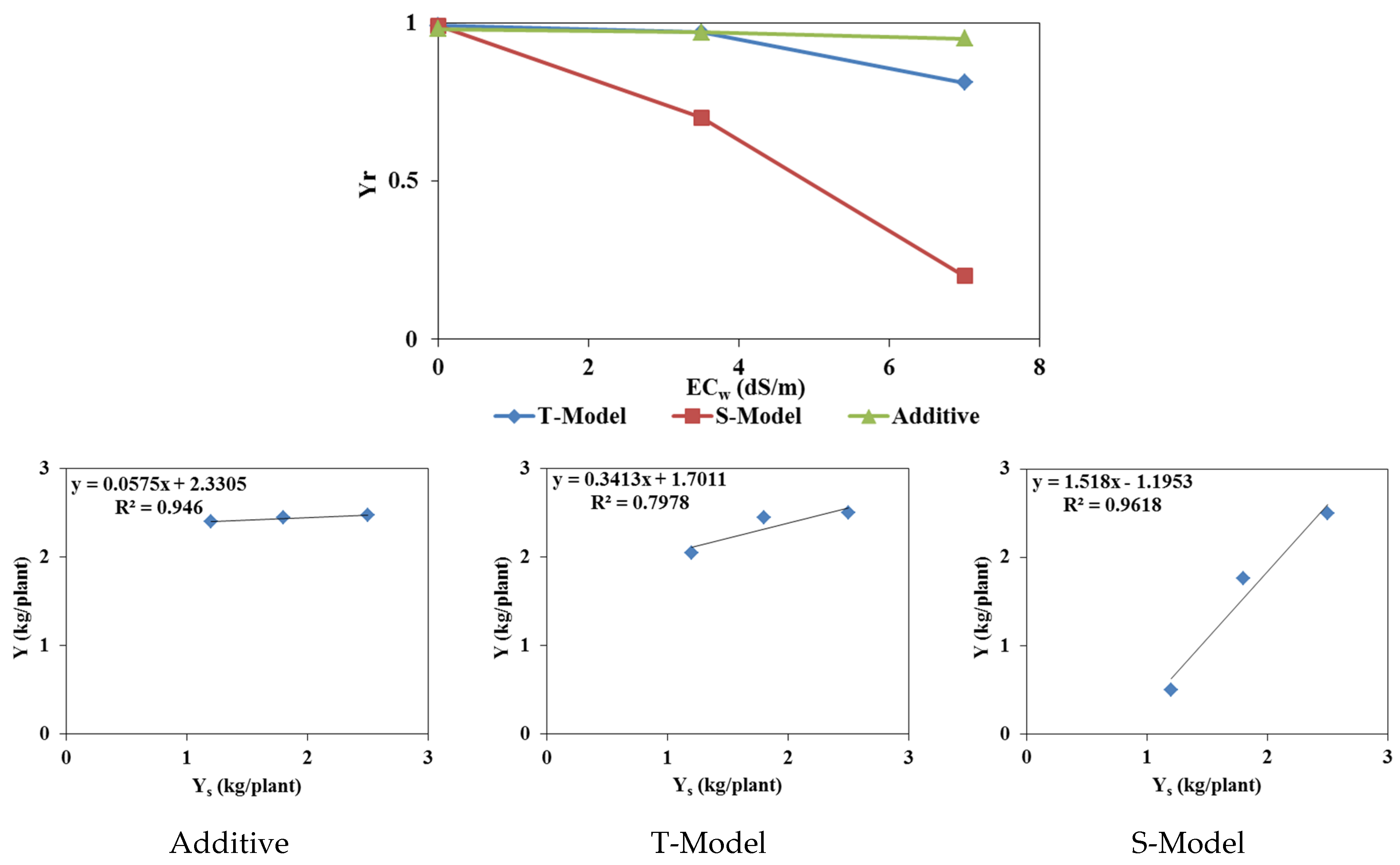
  2. The multiplicative S-model was the best model for reproducing a decrease in tomato relative yield due to irrigation water salinity.
  3. An increase in seasonal temperature of 2°C had no significant effect on tomato yield.

Abstract

:
In arid and semi-arid regions like Tunisia, irrigation water is typically saline, posing a risk of soil and crop salinization and yield reduction. This research aims to study the combined effects of soil matric and osmotic potential stresses on tomato root water uptake. Plants were grown in pot and field experiments in loamy-clay soils and were irrigated with three different irrigation water qualities: 0, 3.5, and 7 dS/m. The Hydrus-1D model was used to simulate the combined dynamics of subsurface soil water and salts. Successful calibration and validation of the model against measured water and salt profiles enabled the examination of the combined effects of osmotic and matric potential stresses on root water uptake. Relative yields, indirectly estimated from actual and potential transpiration, indicated that the multiplicative stress response model effectively simulated the measured yields and the impact of saline water irrigation on crop yields. The experimental and modeling results provide information to aid in determining the salinity levels conducive to optimal crop growth. The findings indicate that the selected salinity levels affect tomato growth to varying degrees. Specifically, the salinity levels conducive to optimal tomato growth were between 0 and 3.5 dS/m, with a significant growth reduction above this salinity level. The gradual salinization of the root zone further evidenced this effect. The scenario considering a temperature increase of 2 °C had no significant impact on crop yields in the pot and field experiments.

1. Introduction

Saline water poses a significant challenge to agricultural sustainability in Tunisia, a country characterized by arid and semi-arid climates. With limited freshwater resources, Tunisia heavily relies on alternative water sources for irrigation, including saline waters (waters containing high concentrations of dissolved salts), which presents both opportunities and challenges for agriculture in Tunisia. The use of saline water for irrigation is widespread in Tunisia, driven by the scarcity of freshwater resources and the increasing demands of agriculture [1]. Saline water sources include groundwater with elevated levels of dissolved salts and treated wastewater from various sources [2]. In some regions, desalination plants have also been established to convert seawater into usable irrigation water [3]. Brackish water requires careful management to avoid negative impacts on soil quality and crop productivity [4,5].
When saline water is applied to the soil, salts accumulate over time, increasing soil salinity levels. It can also contribute to soil erosion and degradation, further exacerbating land degradation issues in Tunisia [6]. In addition to soil salinization, saline water irrigation can directly impact crop health and productivity. Many crops are sensitive to high soil and irrigation water salt concentrations. Excessive salt levels can cause physiological stress in plants, leading to reduced growth, yield losses, and even crop failure [7]. Certain crops, such as tomatoes, are particularly sensitive to salinity stress, making them susceptible to yield reductions when irrigated with saline water [8]. Despite these drawbacks, saline water irrigation also has some benefits for agriculture in Tunisia. Waters containing high concentrations of dissolved salts are often more readily available and less expensive than freshwater sources, providing an alternative water supply for irrigation during water scarcity [9].
Modeling irrigation with saline water is crucial for understanding its effects and implementing effective mitigation strategies. Modeling can be performed using hydrological models, such as Hydrus-1D [10]. These models simulate water movement and solute transport in soils, allowing researchers and farmers to predict how saline water affects soil salinity, crop growth, and yields over time [11]. Using different data for soil hydraulic properties, irrigation practices, and water quality, these models can simulate various scenarios and assess the effectiveness of different management strategies [12]. Modeling can also aid in identifying the most suitable crops for irrigation with water of a given salinity. Indeed, some crops have higher salt tolerance than others, and modeling can help determine which crops are best suited for cultivation in saline environments. Additionally, models can evaluate the impact of different irrigation strategies, such as drip irrigation or leaching, on soil salinity levels and crop productivity [13].
Several models have been developed to simulate water flow and solute transport in soil profiles with plants, such as Hydrus-1D [14,15], SWAP [16], and SALTMOD [17]. In this study, we use the Hydrus-1D model because of its distinct advantages over the other models in modeling root water uptake under various environmental stresses. The Hydrus-1D model offers superior capabilities in simulating water and salt dynamics in the soil profiles with plants under saline irrigation conditions, allowing more accurate predictions of crop responses to varying salinity levels [18,19].
Increased temperatures due to climate change can severely affect tomato production [20]. Increased temperatures can accelerate evaporation, potentially depleting soil moisture [21]. This can negatively impact tomato plants, affecting their growth and yield [22]. Higher temperatures can also alter the phenological stages of tomato plants, affecting flowering, fruit set, and ripening [23]. As temperatures rise, evaporation rates increase, concentrating salts in the soil. This increased soil salinity can adversely affect tomato plants, reducing their ability to absorb water and nutrients, stunting growth, and reducing yields [5].
The objectives of this study are: (i) to integrate the effects of soil matric and osmotic potentials into modeling water and salts transport, (ii) to study the effects of saline water irrigation on tomatoes cultivated under semi-arid conditions to provide a framework for understanding the complex interactions between soil, water, and crops in saline environments, and (iii) to evaluate the effects of an increase in mean air temperature on soil water and salts dynamics and tomatoes’ root water uptake and, ultimately, yield. Haut du formulaire.

2. Materials and Methods

2.1. Experiment Design and Measurements

The experimental trials were conducted on a land parcel (36°51′36.791″ N, 10°11′36.795″ E) in the Ariana region, a semi-arid area in north Tunisia, during the year 2018. The soil is loamy clay. The study focused on a tomato variety, Rio Grande, commonly cultivated in Tunisia. Planting was done on 16 March 2018 in the pot experiment and on 17 April 2018 in the field experiment. A spacing of 25 cm between plants and 50 cm between rows was used in the field experiment. Tomato harvesting occurred on 10 June 2018 in pot cultivation and on 3 August 2018 in field cultivation. Both pot and field experiments were conducted under natural meteorological conditions. The field and pot experimental data are not compared against each other (since they were not carried out at the same time). Instead, they are used to calibrate and validate the Hydrus-1D model and assess its ability to account for environmental stresses.
The water requirements of the crops were estimated using climate data from the past 10-year period obtained from the National Institute of Meteorology. The average values were used to estimate the reference evapotranspiration using the Penman–Monteith formula (FAO-56). For calculating the actual evapotranspiration, crop coefficient values for the three growth stages were taken from those proposed by Allen et al. (1998) [24]. These values are as follows: Kc = 0.6 (initial stage), 1.15 (mid-stage), and 0.8 (final stage). The CROPWAT 8.0 software (FAO, 1998; FAO, 2009) was utilized to establish the irrigation schedule. Water requirements for tomato cultivation are approximately 720 mm.
Surface irrigation was used to deliver water to each individual tomato plant. The irrigation scheduling in the pot and field experiments, mean temperatures, and reference evapotranspiration are presented in Figure 1. No rainfall events were recorded during the tomato growing season. In the field experiments, irrigation was applied every three or four days based on 100% of estimated evapotranspiration (Figure 1). In the pot experiments, irrigation was applied every two or three days until the soil water content reached field capacity (34% in terms of the volumetric soil water content). Soil field capacity was measured using a pressure plate apparatus (for a pressure head of −300 cm). The amounts of water added were recorded for each pot (Figure 1). The average wetted area was 45% in the field experiment and 65% in the pot experiment. Irrigation water provided to the plants had three different qualities: distilled water with a salinity of 0 dS/m, saline water with a salinity of 3.5 dS/m, and saline water with a salinity of 7 dS/m. Volumetric soil water content was measured using the gravimetric method, and soil salinity was measured using the saturated paste extract method [25] with three replicates. In the pot experiment, soil samples were taken every ten days until the end of the tomato plant cycle to characterize soil water and soil salt content. In the field experiment, the soil water content was measured on days 1, 30, 60, and 109 after planting every 20 cm down to a depth of 80 cm.

2.2. Hydrus-1D Model

2.2.1. Theory

Hydrus-1D [14,15] is a numerical model that uses the Galerkin finite element method to solve the Richards equation governing water dynamics in the unsaturated zone:
θ t = z K h z + 1 S
where h is the water pressure head [L], θ is the soil volumetric water content [L3L−3], t is time [T], z is the depth measured from the land surface (positive downward) [L], S is a sink term [L3L−3T−1], and K is the soil unsaturated hydraulic conductivity [LT−1].
Hydrus-1D uses the van Genuchten–Mualem soil hydraulic functions to represent soil hydraulic properties. The soil water retention [26] and hydraulic conductivity [27] functions are as follows:
θ h = θ r + θ s θ r 1 + α h n m h < 0 θ s   h 0
K h = K s S e 0.5 1 1 S e 1 / m m 2
S e = θ θ r θ s θ r
where θr is the residual water content [L3L−3]; θs is the saturated water content [L3L−3]; α [L−1], n (n > 1), and m = 1 − 1/n are shape parameters; Se is the effective saturation; and Ks is the saturated hydraulic conductivity [LT−1].
Hydrus-1D uses the Galerkin finite element method to solve the advection–dispersion equations (ADE) governing solute transport:
θ C t = z θ D C z q θ C z
where C is the solute concentration of the liquid phase [ML−3], D is the dispersion coefficient [L2T−1], and q is the Darcy velocity [LT−1]. When neglecting molecular diffusion, the dispersion coefficient is defined as:
D = λ q
where λ is the soil longitudinal dispersivity [L].
The sink term, S, represents the volume of water removed from a unit volume of soil per unit time due to plant water uptake. The Feddes model, as described by [18], was employed to simulate root water uptake. Three stress response function models available in Hydrus-1D were evaluated for the simulation of salt stress: the additive model (Additive), the threshold model (T-Model), and the S-shape model (S-Model). The last two models are multiplicative models, combining the Feddes model [28], accounting for saturation stress, with either the “Threshold and Slope” model of Mass [29] or the S-shape model of van Genuchten [30], accounting for salinity stress. The theoretical underpinnings of these models are elaborated in the Hydrus-1D manual, with specific parameter values provided for tomato crops.

2.2.2. Soil Hydraulic Properties and Solute Transport Parameters

The estimation of the soil hydraulic parameters, namely the van Genuchten parameters in the water content–pressure head (Equation (2)) and conductivity–saturation (Equation (3)) relationships, was based on soil column evaporation experiments [31].
The dispersion coefficient, a crucial parameter in solute transport in unsaturated soils, cannot be measured, and we thus resorted to indirect methods. Experiments on soil columns were conducted using PVC tubes with a diameter of 15 cm filled with 10 cm of soil. The columns were slowly saturated from the top with distilled water. A Mariotte bottle was placed at the top of the column to maintain a constant pressure head of about 3 cm and steady-state flow conditions. A pulse (50 mL) of a potassium chloride solution (0.8 M, 8.4 dS/m) was manually applied [32,33]. Effluent samples of approximately 100 cm3 were used to measure soil electrical conductivity and determine the solute breakthrough curve (BTC). The experimental BTC values were fitted using the analytical solution of the ADE using CXTFIT 2.1 software [34] to estimate the dispersion coefficient.

2.2.3. Model Calibration and Validation

The Hydrus-1D model was calibrated using measured soil water content and salinity profiles in both pots and field experiments irrigated with fresh water (i.e., 0 dS/m). The validation of the Hydrus-1D model was carried out by keeping the same input parameters and only changing the water quality in both cases of this study (pot and field experiments).

2.3. Statistical Evaluation of Modeling Results

Simulation results were evaluated graphically and statistically. In the graphical method, the measured and simulated volumetric water content values were plotted as a function of soil depth. The statistical approach involved calculating the root mean square error (RMSE; in %):
R M S E = i = 1 n ( s i m i ) ² n × 1 m ¯ × 100
where si is the simulated value, mi is the measured value, m ¯ is the average observed value, and n is the number of observations.

3. Results and Discussion

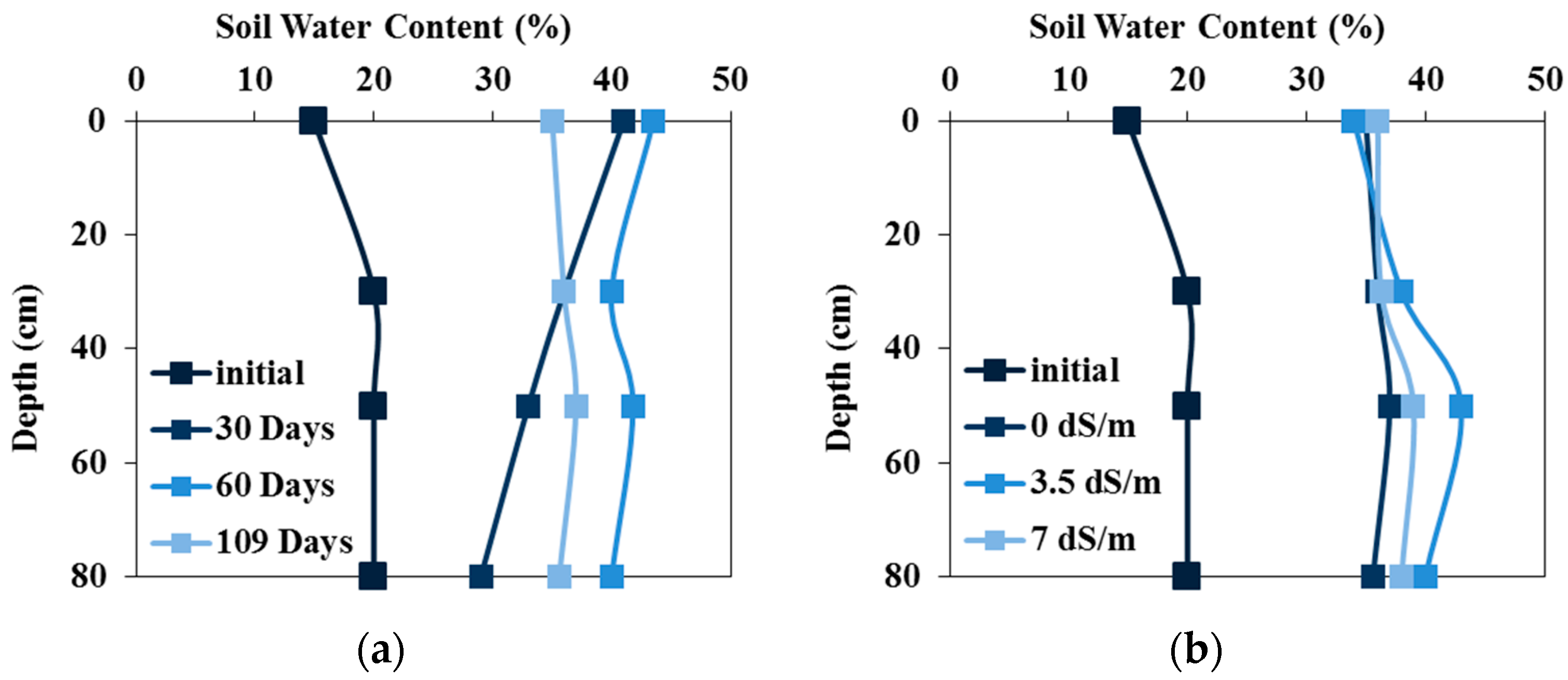
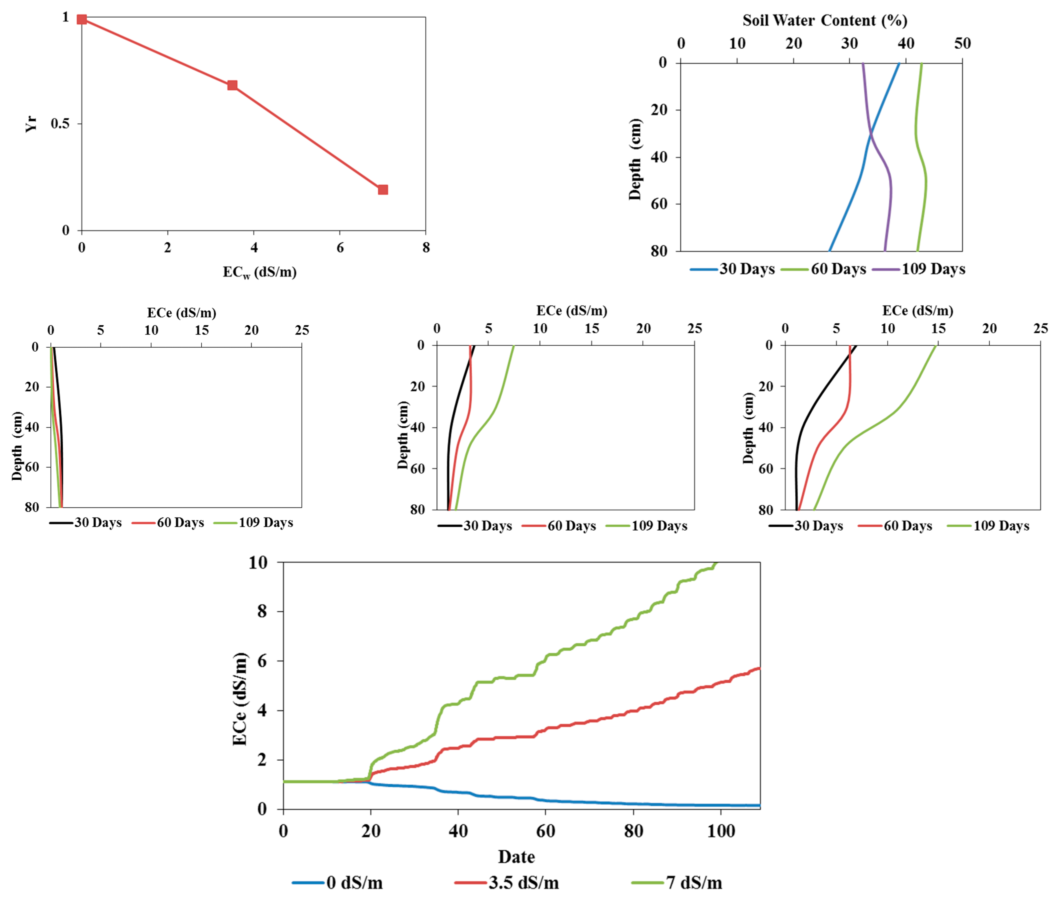
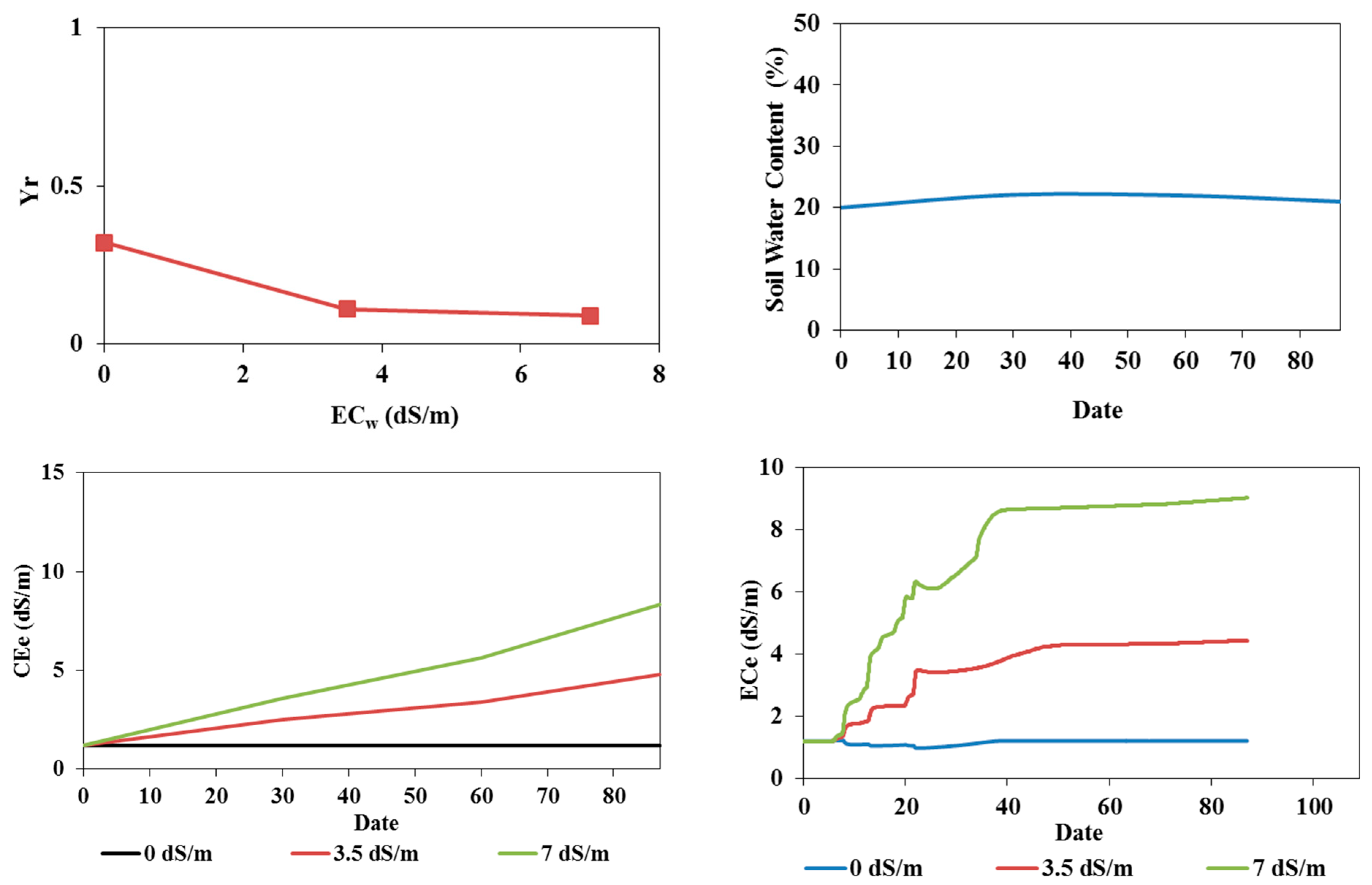
3.1. Soil Water Content Dynamics

The variations in the soil water content in the pot experiments are presented in Figure 2. During the first month after the start of irrigation, the water content gradually increased to reach the field capacity (34%) in all three pots irrigated with different water qualities [35,36,37]. The water content of the soil irrigated with the saltiest water (7 dS/m) remained at the field capacity. As the soil salinity increased with frequent irrigations, osmotic pressure also increased, preventing root water uptake. Irrigations with the other two water qualities did not block water extraction by the plant roots, and the soil water content decreased over time. The soil irrigated with fresh water (0 dS/m) had the lowest water content values, as the plant roots extracted water without any osmotic potential constraints.
The soil water profiles, measured every 30 days in the field experiment with tomatoes irrigated with fresh water, are illustrated in Figure 3a. This figure shows the variations in soil water content without significant osmotic potential effects. Indeed, the soil water content profiles show dynamics that reflect infiltration (wetting) and evaporation (drying) episodes. After 109 irrigation days, the water content exceeded the field capacity, indicating that the roots did not undergo water stress.
Figure 3b shows the water content profiles measured after 109 irrigation days in field experiments irrigated with waters of different qualities. The water content in the surface layers is very close to field capacity (34%), while it increases considerably with depth, indicating deep water infiltration. The irrigation strategy based on calculating the water needs using climatic parameters from the previous ten years to estimate actual evapotranspiration succeeded in not subjecting the crop to water stress [38]. However, deep percolation shows that crop water needs were overestimated [39].

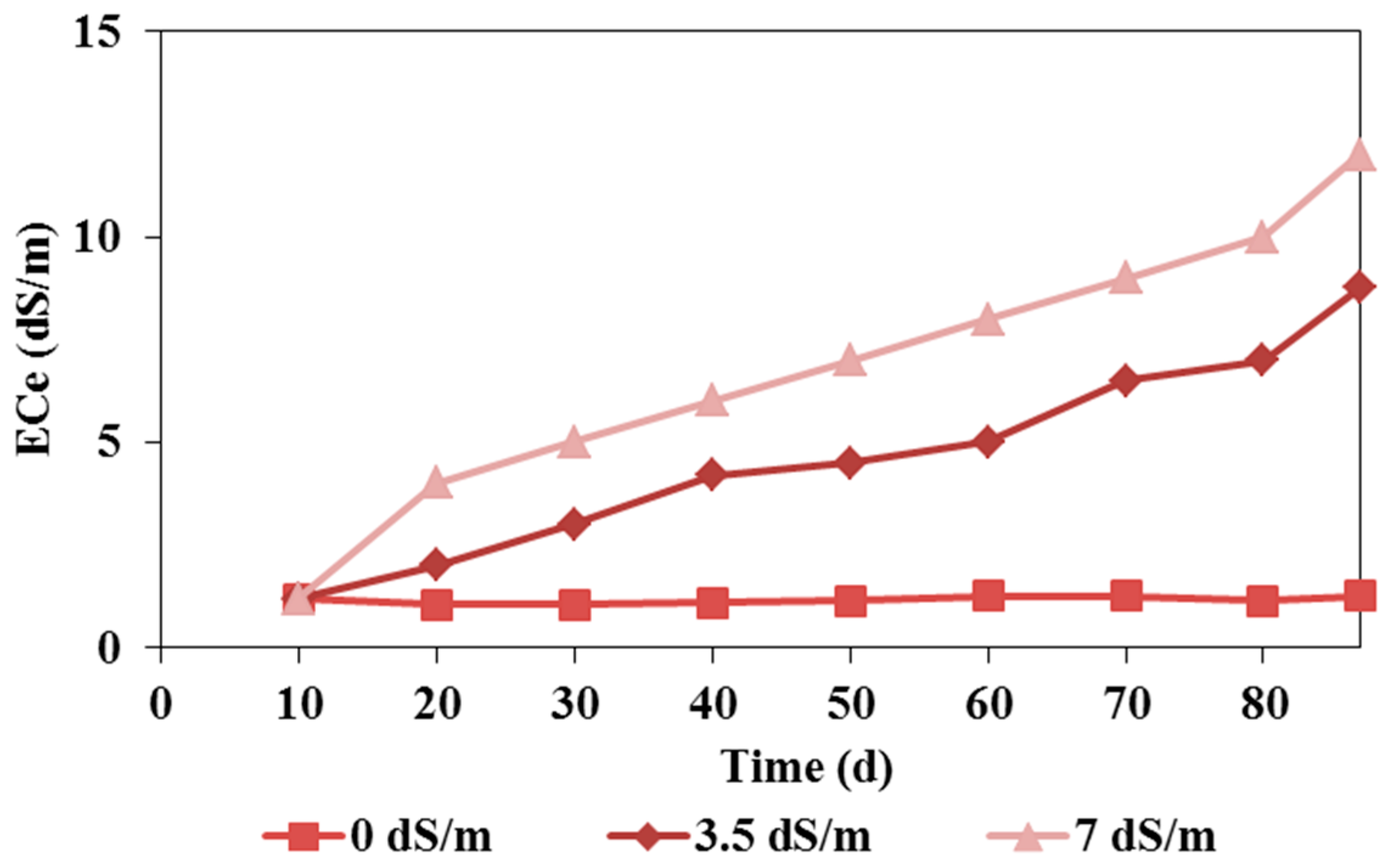
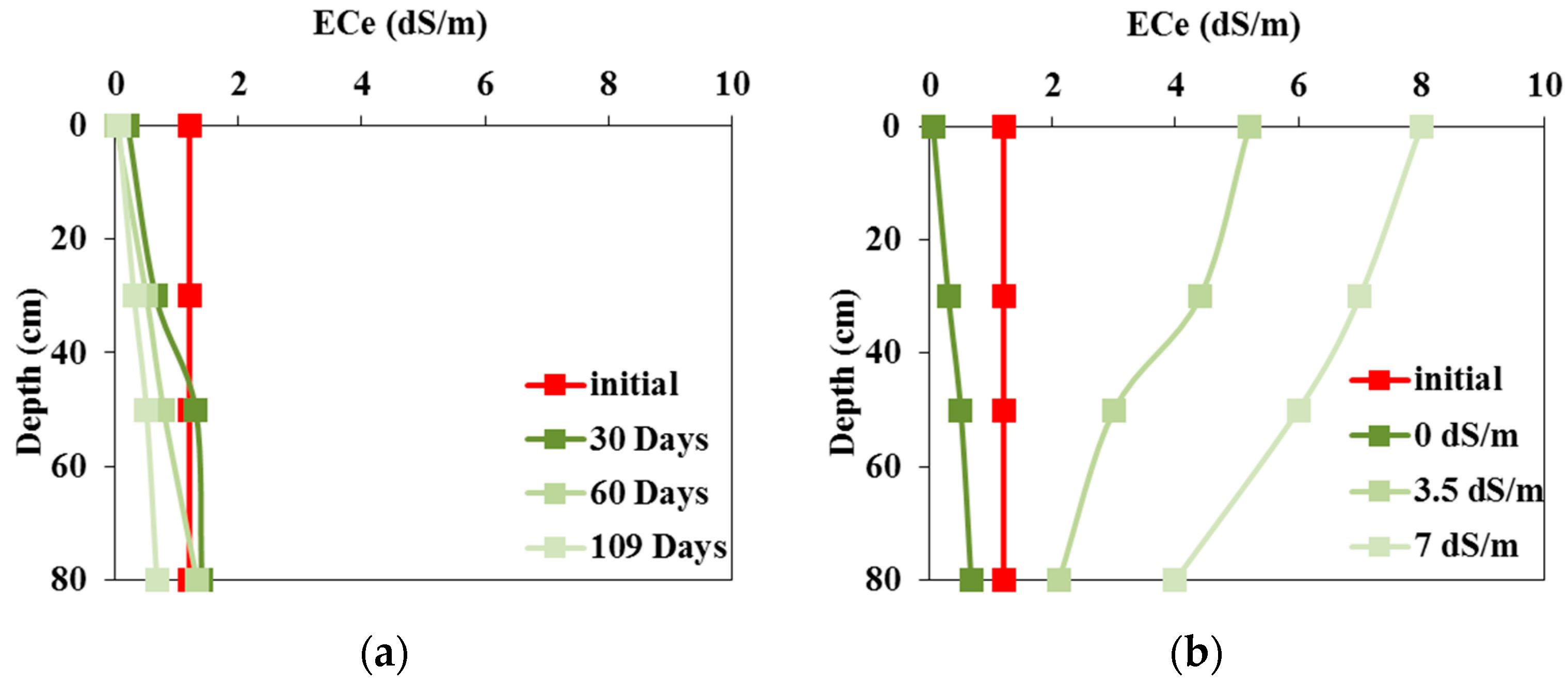
3.2. Soil Salinity Dynamics

The variations in the average soil salinity in the pot experiments irrigated with waters of different qualities are shown in Figure 4. This figure shows a nearly constant level of salinity in soils irrigated with fresh water and a gradual increase in soil salinity in soils irrigated with lower-quality waters, reaching 8 dS/m when 3.5 dS/m water was used and 12 dS/m when 7 dS/m water was used.
In the field experiment irrigated with fresh water, the variations in the soil salinity profiles measured every thirty days indicated continuous leaching of the initial salinity (Figure 5a). In contrast, surface salinity significantly increased during irrigations with saline waters of 3.5 dS/m and 7 dS/m, reaching 7 dS/m and 12 dS/m, respectively, at the end of the crop cycle (Figure 5b). Soil salinity is higher near the surface than at depth, mainly due to evapotranspiration causing salt accumulation near the soil surface [40].

3.3. Numerical Modeling of Water and Salt Dynamics with Root Water Uptake

3.3.1. Inputs to Hydrus-1D

The soil was considered homogeneous in pot experiments, consisting of a single layer of 30 cm. In the field experiment, water content and salinity measurements were taken every 20 cm down to a depth of 80 cm. Four soil layers (horizons) of 20 cm thickness were considered in the simulations. The values of the van Genuchten–Mualem parameters for the four soil layers are presented in Table 1. The simulation period lasted 87 days in the pot experiments, with three output dates of 30, 60, and 87 days. On the other hand, the field trial lasted 109 days, and the output dates were 30, 60, and 109 days.
The dispersivity of the different soil layers varied around 5 cm, except for the 60–80 cm layer, where it was equal to 3 cm. The distribution coefficient of the adsorption isotherm ranged between 0.1 g/cm3 and 0.3 g/cm3 for all soil layers. Hydrus-1D includes a database that provides stress response function values for many crops, including tomatoes, which were considered here. The initial soil water content and soil salinity values as a function of depth in the field experiment are shown in Figure 6. In the pot experiment, the initial water content was 20%, and the initial soil salinity was 1.2 dS/m.
For the simulation of field experiments, we used the rainfall and evapotranspiration data from the National Institute of Meteorology and crop coefficients from [24].

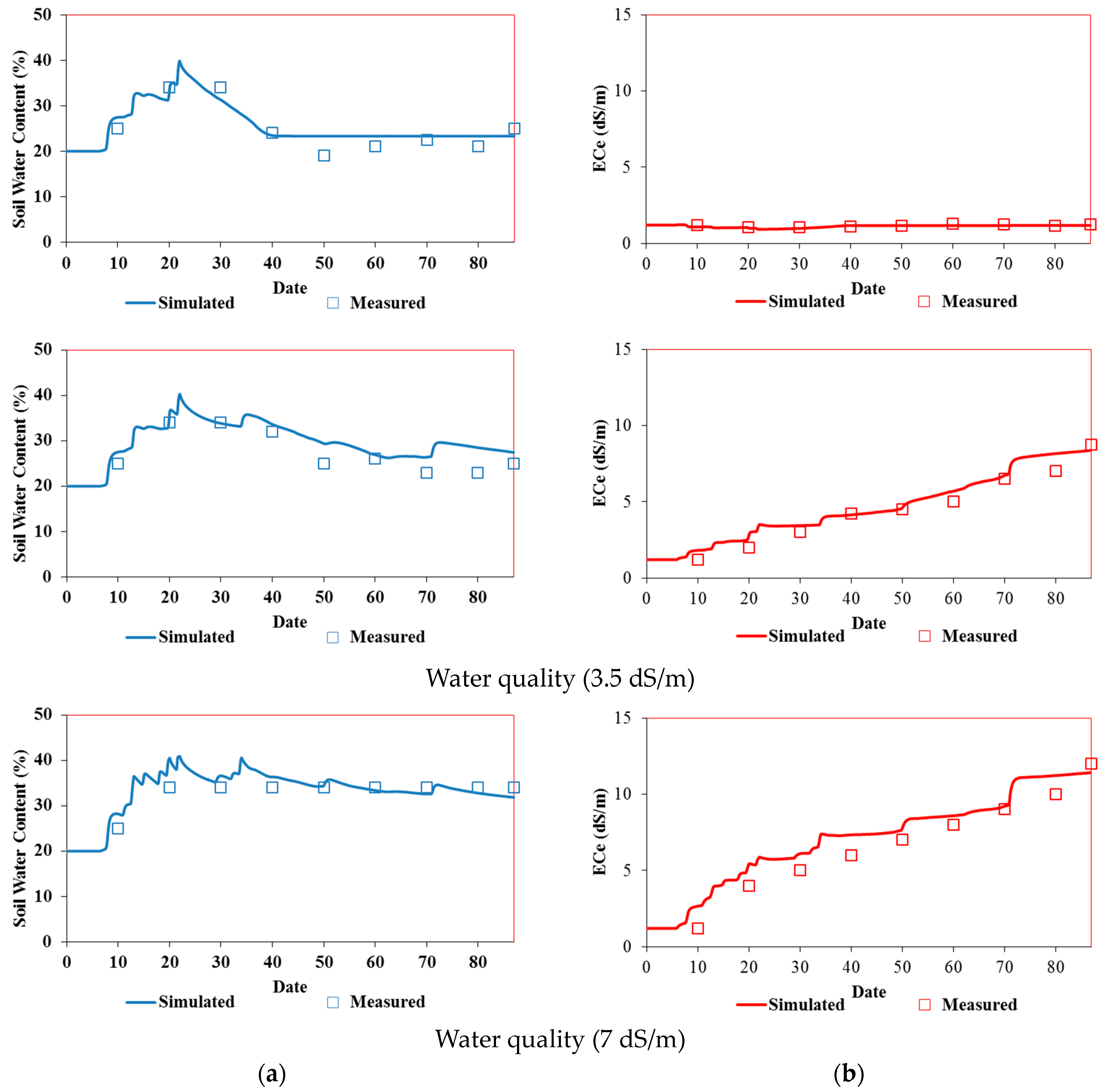
3.3.2. Simulation Results

The Hydrus-1D model was used to simulate the movement of water and salts in both pot and field soils, considering root water uptake under the combined effects of soil matric and osmotic potentials.

Model Calibration

The Hydrus-1D model was calibrated using measured soil water content and salinity profiles in both pots and field experiments irrigated with fresh water (i.e., 0 dS/m). The measured and simulated water content and salinity values for both experiments are presented in Figure 7, Figure 8 and Figure 9. The measured soil water content values are quite close to the simulated values. In the field experiment (Figure 7 and Figure 8), the Hydrus-1D model underestimated the measured water content on day 30 and overestimated it on the other output dates. The model slightly overestimated the volumetric water content in the pot experiment (Figure 9).
The measured soil salinity profiles during the two pot and field experiments with tomatoes irrigated with saline waters and simulated using the Hydrus-1D model are presented in Figure 9. Overall, the measured and simulated values are similar on all three output dates. The simulated soil electrical conductivities generally overestimated the measured values in both experiments.

Model Validation

The validation of the Hydrus-1D model was carried out by keeping the same input parameters and only changing the water quality in both cases of this study (pot and field experiments). Figure 6 and Figure 7 show that the simulated soil water content profiles agree well with the measured profiles for both pot and field experiments. Indeed, for all the output dates, the simulated profiles are very close to the measured ones.
The model’s performance was evaluated qualitatively (Figure 7, Figure 8 and Figure 9) and assessed using statistical evaluations and the RMSE values (Table 2 and Table 3). These values are low (<10%) and highlight the model’s reliability for simulating water and salt dynamics for both experiments and during the calibration and validation processes [41].

3.3.3. Crop Yield

The Hydrus-1D model cannot directly estimate the crop yield. However, according to Oster et al. (2012), the relative yield (Yr) can be estimated as the ratio between the actual and potential (or maximum) transpiration, which are both provided in the model’s output files [42]. Figure 10 and Figure 11 show the relative yields for tomatoes irrigated with waters of different qualities for both experimental pot and field trials simulated using the three models mentioned above (Additive, T-Model, and S-Model) to represent the effects of osmotic and matric potentials on crop root water uptake. The simulated relative yields decreased with increased irrigation water salinity (ECw) for all three stress response functions (Figure 10). The relative yield is 0.98 in the field experiment with tomatoes irrigated with fresh water (0 dS/m) for all three stress response functions. However, in the pot case, Yr equals 0.33 for freshwater irrigation. The reduced root development in pots compared to the field accounts for this reduction in relative yield [43].
The actual yields measured in the two trials with different irrigation water qualities were compared to the simulated yields to identify the most suitable stress response function model for studying the combined effects of osmotic and matric potentials. According to FAO Note 66 (2012), Yr = Y/Ymax, where Y is the actual yield, and Ymax is the maximum (or potential) yield. In our experiments, Ymax is calculated for irrigations with fresh water. The Ymax value equals 2.53 kg/plant for the field experiment and 4.16 kg/plant for the pot trial. The values of the simulated relative yields were calculated using these values [42].
Figure 10 and Figure 11 also present linear correlations between the measured and simulated relative yields. The relative yields simulated using the additive model (Feddes) and the multiplicative T-Model (combining the Feddes et al. [28] model for saturation stress with the threshold and slope model of Mass [29] for osmotic stress) were least correlated with the measured relative yields in both pot and field trials. The multiplicative S-Model (combining the Feddes model [28] for saturation stress with the S-shape model of van Genuchten [30] for osmotic stress) is the only model capable of reproducing the measured relative yields with a correlation coefficient R² close to 1 for both pot and field experiments.

3.4. Effect of Temperature Increase

According to the IPCC (2021), temperatures in Tunisia are expected to increase by 2 °C over the coming decades. The effects of this temperature increase on tomato cultivation were studied (numerically) by increasing the temperature by 2 °C. To this aim, the reference evapotranspiration (ET0) values were recalculated, and simulations were rerun using the updated ET0 values while all other model parameters were kept unchanged.
The results of these simulations are presented in Figure 12 and Figure 13. In the field experiment, soil water content exceeded field capacity in the root zone. In deeper layers between 40 and 80 cm, soil water content decreased after the 60th day, indicating infiltration beyond the root zone. On the other hand, in the pot experiment, the water content remained constant and below field capacity. Additionally, the accumulation of salts in the surface layer increased due to irrigation with saline waters and increased evaporation. The salinity in the root zone reached an average value of 6 dS/m, and the relative yields estimated using the S-Model did not change compared to the measured relative yields. An increase in temperature, thus, did not significantly affect the tomato yields in either trial [20].

4. Conclusions

The aridity of regions like Tunisia has prompted the intensification of irrigation practices. However, the scarcity of good-quality water resources has led to the necessity of using brackish water in agriculture. The accumulation of salts due to irrigation with such waters has detrimental effects on both soil and crop yields. Experiments conducted using tomatoes grown in pots and the field and irrigated with three different water qualities ranging in salinity from 0 dS/m to 7 dS/m provided data to study the variations in soil water and salt dynamics. In both pot and field trials, the water content in the root zone (0–30 cm) remained close to field capacity throughout the crop cycle. The variations in salt profiles showed progressive soil salinization depending on irrigation water salinity, reaching 12 dS/m in the pot soil and 8 dS/m in the field soil. Crop reactions to these water qualities were evaluated using water movement and salt transfer modeling using the Hydrus-1D model. The combined effects of osmotic and matric potentials were evaluated using three stress response function models: the additive model and two multiplicative models, the T-Model and S-Model. The estimated relative crop yields showed that only the S-Model could reproduce the measured relative yields. A hypothetical 2 °C temperature increase did not significantly affect crop yields. Soil salinization slightly increased due to increased temperature and evaporation.
Adopting a modeling approach based on soil geochemical characterization and the UnsatChem module of HYDRUS [14,15], which considers transport and reactions between major ions (e.g., Ca2+, Mg2+, Na+, K+, SO42− CO32−, Cl), would be an alternative approach to this study, where the risks of soil alkalization and salinization could be more thoroughly explored for strategic crops like tomatoes. Moreover, to obtain more accurate yield predictions, using specialized crop models, such as AquaCrop and DSSAT, would be advisable. These crop models are specifically designed to simulate and predict crop growth and yield under varying environmental conditions and provide more reliable estimates of agricultural productivity. Therefore, while Hydrus-1D excels in soil water and salinity dynamics, including crop models such as AquaCrop and DSSAT would improve the accuracy of yield predictions.

Author Contributions

Conceptualization, S.K., I.D. and K.B.A.; Data curation, S.K., K.B.A., S.B.M. and S.G.; Formal analysis, S.K., J.Š. and S.B.M.; Funding acquisition, S.K. and S.B.M.; Investigation, S.K., J.Š., I.D., A.Y., K.B.A., S.B.M. and S.G.; Project administration, S.K. and S.B.M.; Resources, S.K. and S.B.M.; Software, J.Š.; Supervision, S.K. and S.B.M.; Visualization, S.K., J.Š., I.D., A.Y., K.B.A., S.B.M. and S.G.; Writing—original draft, S.K. and J.Š.; Writing—review and editing, S.K., J.Š., I.D., A.Y., K.B.A., S.B.M. and S.G. All authors have read and agreed to the published version of the manuscript.

Funding

This research received no external funding.

Data Availability Statement

The data supporting the findings of this research are available in the manuscript.

Conflicts of Interest

The authors declare no conflict of interest.

References

  1. Besser, H.; Dhaouadi, L.; Hadji, R.; Hamed, Y.; Jemmali, H. Ecologic and Economic Perspectives for Sustainable Irrigated Agriculture under Arid Climate Conditions: An Analysis Based on Environmental Indicators for Southern Tunisia. J. Afr. Earth Sci. 2021, 177, 104134. [Google Scholar] [CrossRef]
  2. Srivastava, A.; Parida, V.K.; Majumder, A.; Gupta, B.; Gupta, A.K. Treatment of Saline Wastewater Using Physicochemical, Biological, and Hybrid Processes: Insights into Inhibition Mechanisms, Treatment Efficiencies and Performance Enhancement. J. Environ. Chem. Eng. 2021, 9, 105775. [Google Scholar] [CrossRef]
  3. Martínez-Alvarez, V.; González-Ortega, M.J.; Martin-Gorriz, B.; Soto-García, M.; Maestre-Valero, J.F. The Use of Desalinated Seawater for Crop Irrigation in the Segura River Basin (South-Eastern Spain). Desalination 2017, 422, 153–164. [Google Scholar] [CrossRef]
  4. Qadir, M.; Oster, J.D. Crop and Irrigation Management Strategies for Saline-Sodic Soils and Waters Aimed at Environmentally Sustainable Agriculture. Sci. Total Environ. 2004, 323, 1–19. [Google Scholar] [CrossRef]
  5. Muhammad, M.; Waheed, A.; Wahab, A.; Majeed, M.; Nazim, M.; Liu, Y.-H.; Li, L.; Li, W.-J. Soil Salinity and Drought Tolerance: An Evaluation of Plant Growth, Productivity, Microbial Diversity, and Amelioration Strategies. Plant Stress 2024, 11, 100319. [Google Scholar] [CrossRef]
  6. Deeb, M.; Smagin, A.V.; Pauleit, S.; Fouché-Grobla, O.; Podwojewski, P.; Groffman, P.M. The Urgency of Building Soils for Middle Eastern and North African Countries: Economic, Environmental, and Health Solutions. Sci. Total Environ. 2024, 917, 170529. [Google Scholar] [CrossRef] [PubMed]
  7. El-Ramady, H.; Prokisch, J.; Mansour, H.; Bayoumi, Y.A.; Shalaby, T.A.; Veres, S.; Brevik, E.C. Review of Crop Response to Soil Salinity Stress: Possible Approaches from Leaching to Nano-Management. Soil Syst. 2024, 8, 11. [Google Scholar] [CrossRef]
  8. Li, J.; Chen, J.; He, P.; Chen, D.; Dai, X.; Jin, Q.; Su, X. The Optimal Irrigation Water Salinity and Salt Component for High-Yield and Good-Quality of Tomato in Ningxia. Agric. Water Manag. 2022, 274, 107940. [Google Scholar] [CrossRef]
  9. Khondoker, M.; Mandal, S.; Gurav, R.; Hwang, S. Freshwater Shortage, Salinity Increase, and Global Food Production: A Need for Sustainable Irrigation Water Desalination—A Scoping Review. Earth 2023, 4, 223–240. [Google Scholar] [CrossRef]
  10. Li, P.; Ren, L. Evaluating the Saline Water Irrigation Schemes Using a Distributed Agro-Hydrological Model. J. Hydrol. 2021, 594, 125688. [Google Scholar] [CrossRef]
  11. Yu, Q.; Kang, S.; Hu, S.; Zhang, L.; Zhang, X. Modeling Soil Water-Salt Dynamics and Crop Response under Severely Saline Condition Using WAVES: Searching for a Target Irrigation Volume for Saline Water Irrigation. Agric. Water Manag. 2021, 256, 107100. [Google Scholar] [CrossRef]
  12. Kanzari, S.; Jaziri, R.; Ali, K.B.; Daghari, I. Long-Term Evaluation of Soil Salinization Risks under Different Climate Change Scenarios in a Semi-Arid Region of Tunisia. Water Supply 2021, 21, 2463–2476. [Google Scholar] [CrossRef]
  13. Majeed, A.; Stockle, C.O.; King, L.G. Computer Model for Managing Saline Water for Irrigation and Crop Growth: Preliminary Testing with Lysimeter Data. Agric. Water Manag. 1994, 26, 239–251. [Google Scholar] [CrossRef]
  14. Šimůnek, J.; van Genuchten, M.T.; Šejna, M. Recent Developments and Applications of the HYDRUS Computer Software Packages. Vadose Zone J. 2016, 15, 1–25. [Google Scholar] [CrossRef]
  15. Šimůnek, J.; Brunetti, G.; Jacques, D.; van Genuchten, M.T.; Šejna, M. Recent developments and applications of the HYDRUS computer software packages since 2016. Vadose Zone J. 2024, 23, e20310. [Google Scholar]
  16. van Dam, J.C.; Groenendijk, P.; Hendriks, R.F.A.; Kroes, J.G. Advances of Modeling Water Flow in Variably Saturated Soils with SWAP. Vadose Zone J. 2008, 7, 640–653. [Google Scholar] [CrossRef]
  17. Miao, Q.; Rosa, R.D.; Shi, H.; Paredes, P.; Zhu, L.; Dai, J.; Gonçalves, J.M.; Pereira, L.S. Modeling Water Use, Transpiration and Soil Evaporation of Spring Wheat–Maize and Spring Wheat–Sunflower Relay Intercropping Using the Dual Crop Coefficient Approach. Agric. Water Manag. 2016, 165, 211–229. [Google Scholar] [CrossRef]
  18. Kumar, P.; Sarangi, A.; Singh, D.K.; Parihar, S.S.; Sahoo, R.N. Simulation of Salt Dynamics in the Root Zone and Yield of Wheat Crop under Irrigated Saline Regimes Using SWAP Model. Agric. Water Manag. 2015, 148, 72–83. [Google Scholar] [CrossRef]
  19. Kanzari, S.; Daghari, I.; Šimůnek, J.; Younes, A.; Ilahy, R.; Ben Mariem, S.; Rezig, M.; Ben Nouna, B.; Bahrouni, H.; Ben Abdallah, M.A. Simulation of Water and Salt Dynamics in the Soil Profile in the Semi-Arid Region of Tunisia—Evaluation of the Irrigation Method for a Tomato Crop. Water 2020, 12, 1594. [Google Scholar] [CrossRef]
  20. Ploeg, D.V.; Heuvelink, E. Influence of Sub-Optimal Temperature on Tomato Growth and Yield: A Review. J. Hortic. Sci. Biotechnol. 2005, 80, 652–659. [Google Scholar] [CrossRef]
  21. Bhandari, R.; Neupane, N.; Adhikari, D.P. Climatic Change and Its Impact on Tomato (Lycopersicum esculentum L.) Production in Plain Area of Nepal. Environ. Chall. 2021, 4, 100129. [Google Scholar] [CrossRef]
  22. Petrović, I.; Savić, S.; Gricourt, J.; Causse, M.; Jovanović, Z.; Stikić, R. Effect of Long-Term Drought on Tomato Leaves: The Impact on Metabolic and Antioxidative Response. Physiol. Mol. Biol. Plants 2021, 27, 2805–2817. [Google Scholar] [CrossRef]
  23. Delgado-Vargas, V.A.; Ayala-Garay, O.J.; Arévalo-Galarza, M.d.L.; Gautier, H. Increased Temperature Affects Tomato Fruit Physicochemical Traits at Harvest Depending on Fruit Developmental Stage and Genotype. Horticulturae 2023, 9, 212. [Google Scholar] [CrossRef]
  24. Allen, R.G.; Pereira, L.S.; Raes, D.; Smith, M. Crop evapotranspiration: Guide-lines for computing crop water requirements. In FAO Irrigation and Drainage Paper No. 56; FAO: Rome, Italy, 1998; 300p. [Google Scholar]
  25. Hide, J.C. Diagnosis and Improvement of Saline and Alkali Soils. U.S. Salinity Laboratory Staff; L. A. Richards, Ed. U.S. Dept. of Agriculture, Washington, D.C., Rev. Ed., 1954. Vii + 160 Pp. Illus. $2. (Order from Supt. of Documents, GPO, Washington 25, D.C.). Science 1954, 120, 800. [Google Scholar] [CrossRef]
  26. van Genuchten, M.T. A Closed-Form Equation for Predicting the Hydraulic Conductivity of Unsaturated Soils. Soil Sci. Soc. Am. J. 1980, 44, 892–898. [Google Scholar] [CrossRef]
  27. Mualem, Y. A New Model for Predicting the Hydraulic Conductivity of Unsaturated Porous Media. Water Resour. Res. 1976, 12, 513–522. [Google Scholar] [CrossRef]
  28. Feddes, R.A.; Kowalik, P.J.; Zaradny, H. Simulation of Field Water Use And Crop Yield. In Simulation Monographs; Pudoc: Wageningen, The Netherlands, 1978; p. 189. [Google Scholar]
  29. Maas, E.V. Crop salt tolerance. In Agricultural Salinity Assessment and Management; Tanji, K.K., Ed.; ASCE Manuals and Reports on Engineering Practice: New York, NY, USA, 1990; Volume 71. [Google Scholar]
  30. van Genuchten, M.T. A Numerical Model for Water and Solute Movement in and Below the Root Zone, Unpublished Research Report; U.S. Salinity Laboratory, USDA, ARS: Riverside, CA, USA, 1987. [Google Scholar]
  31. Kanzari, S.; Rezig, M.; Ben Nouna, B. Estimating Hydraulic Properties of Unsaturated Soil Using a Single Tensiometer. Am. J. Geophys. Geochem. Geosystems 2017, 3, 1–4. [Google Scholar]
  32. Vanclooster, M.; Mallants, D.; Diels, J.; Feyen, J. Determining Local-Scale Solute Transport Parameters Using Time Domain Reflectometry (TDR). J. Hydrol. 1993, 148, 93–107. [Google Scholar] [CrossRef]
  33. Mallants, D.; Vanclooster, M.; Meddahi, M.; Feyen, J. Estimating Solute Transport in Undisturbed Soil Columns Using Time-Domain Reflectometry. J. Contam. Hydrol. 1994, 17, 91–109. [Google Scholar] [CrossRef]
  34. Toride, N.; Leij, F.J.; van Genuchten, M.T. The CXTFIT Code for Estimating Transport Parameters from Laboratory or Field Tracer Experiment. Research Report N°137; US Salinity Laboratory: Riverside, CA, USA, 1999; p. 119. [Google Scholar]
  35. Carucci, F.; Gagliardi, A.; Giuliani, M.M.; Gatta, G. Irrigation Scheduling in Processing Tomato to Save Water: A Smart Approach Combining Plant and Soil Monitoring. Appl. Sci. 2023, 13, 7625. [Google Scholar] [CrossRef]
  36. Zhang, J.; Xiang, L.; Zhu, C.; Li, W.; Jing, D.; Zhang, L.; Liu, Y.; Li, T.; Li, J. Evaluating the Irrigation Schedules of Greenhouse Tomato by Simulating Soil Water Balance under Drip Irrigation. Agric. Water Manag. 2023, 283, 108323. [Google Scholar] [CrossRef]
  37. Shan, G.; Sun, Y.; Cheng, Q.; Wang, Z.; Zhou, H.; Wang, L.; Xue, X.; Chen, B.; Jones, S.B.; Lammers, P.S.; et al. Monitoring Tomato Root Zone Water Content Variation and Partitioning Evapotranspiration with a Novel Horizontally-Oriented Mobile Dielectric Sensor. Agric. For. Meteorol. 2016, 228–229, 85–94. [Google Scholar] [CrossRef]
  38. Gassmann, M.; Gardiol, J.; Serio, L. Performance Evaluation of Evapotranspiration Estimations in a Model of Soil Water Balance. Meteorol. Appl. 2011, 18, 211–222. [Google Scholar] [CrossRef]
  39. Abou Ali, A.; Bouchaou, L.; Er-Raki, S.; Hssaissoune, M.; Brouziyne, Y.; Ezzahar, J.; Khabba, S.; Chakir, A.; Labbaci, A.; Chehbouni, A. Assessment of Crop Evapotranspiration and Deep Percolation in a Commercial Irrigated Citrus Orchard under Semi-Arid Climate: Combined Eddy-Covariance Measurement and Soil Water Balance-Based Approach. Agric. Water Manag. 2023, 275, 107997. [Google Scholar] [CrossRef]
  40. Liu, S.; Huang, Q.; Ren, D.; Xu, X.; Xiong, Y.; Huang, G. Soil Evaporation and Its Impact on Salt Accumulation in Different Landscapes under Freeze–Thaw Conditions in an Arid Seasonal Frozen Region. Vadose Zone J. 2021, 20, e20098. [Google Scholar] [CrossRef]
  41. Mai, J. Ten Strategies towards Successful Calibration of Environmental Models. J. Hydrol. 2023, 620, 129414. [Google Scholar] [CrossRef]
  42. Oster, J.D.; Letey, J.; Vaughan, P.; Wu, L.; Qadir, M. Comparison of Transient State Models That Include Salinity and Matric Stress Effects on Plant Yield. Agric. Water Manag. 2012, 103, 167–175. [Google Scholar] [CrossRef]
  43. Poorter, H.; Bühler, J.; van Dusschoten, D.; Climent, J.; Postma, J.A. Pot Size Matters: A Meta-Analysis of the Effects of Rooting Volume on Plant Growth. Funct. Plant Biol. 2012, 39, 839–850. [Google Scholar] [CrossRef]
Figure 1. Mean temperatures, reference evapotranspiration (top), and tomato irrigation scheduling (bottom) in the pot and field experiments.
Land 13 00739 g001aLand 13 00739 g001b
Figure 2. Measured soil water content (in %) in the pot experiments irrigated with different water qualities (0, 3, and 7 dS/m).
Land 13 00739 g002
Figure 3. Measured soil water content (in %) in the field experiments with tomatoes irrigated with (a) fresh water (at 30, 60, and 109 d) and (b) waters of different salinities (0, 3, and 7 dS/m) (at 109 days).
Land 13 00739 g003
Figure 4. Soil salt content (ECe) in the pot experiments irrigated with waters of different salinities (0, 3, and 7 dS/m).
Land 13 00739 g004
Figure 5. Measured soil salt content in the field experiments with tomatoes irrigated with (a) fresh water (at 30, 60, and 109 d) and (b) waters of different salinities (0, 3, and 7 dS/m) (at 109 days).
Land 13 00739 g005
Figure 6. Measured initial (a) water content and (b) salinity as a function of soil depth in the field experiment.
Land 13 00739 g006
Figure 7. Measured and simulated (calibration) soil water content (in %) (top) and salinity (in dS/m) (bottom) in the field experiment irrigated with fresh water at 30 (left), 60 (middle), and 109 (right) days.
Land 13 00739 g007
Figure 8. Measured and simulated (validation) soil water content (in %; (top)) and salinity (in dS/m; (bottom)) in the field experiments irrigated with saline waters of 3.5 dS/m (left) and 7 dS/m (right) at the end of the experiment.
Land 13 00739 g008
Figure 9. Measured and simulated time series of soil water content (%) (left) and salinity (dS/m) (right) in the pot experiments irrigated with (a) freshwater (top) (calibration) and (b) saline waters of 3.5 dS/m (middle) and 7 dS/m (bottom) (validation).
Land 13 00739 g009
Figure 10. The effect of saline irrigation water on tomatoes’ relative yield (Yr) [−] (top) and the relationships between the actual (Y) and simulated (Ys) yields (kg/plant) (bottom) using the three stress response models (Additive, T-Model, and S-Model) incorporated in Hydrus-1D (field experiments).
Land 13 00739 g010
Figure 11. The effect of saline irrigation water on tomatoes’ relative yield (Yr) [−] (top) and the relationships between the actual (Y) and simulated (Ys) yields (kg/plant) (bottom) using the three stress response models (Additive, T-Model, and S-Model) incorporated in Hydrus-1D (pot experiments).
Land 13 00739 g011
Figure 12. Effects of a temperature increase of 2 °C on tomatoes cultivated in field conditions: relative yield as a function of irrigation water salinity (top left); soil water content profiles at 30, 60, and 109 days when irrigated with freshwater (top right); soil salinity profiles at 30, 60, and 109 days (middle row) when irrigated with fresh water (left) and saline waters of 3.5 (middle) and 7 (right) dS/m; and average root zone salinity when irrigated with fresh water and saline waters of 3.5 and 7 dS/m (bottom).
Land 13 00739 g012
Figure 13. Effects of a temperature increase of 2 °C on tomatoes cultivated in pot conditions: relative yield as a function of irrigation water salinity (top left); average soil water content when irrigated with fresh water (top right); average soil salinity in the 0–30 cm soil layer (bottom left); and root zone salinity (at 5 cm depth) for irrigations with fresh water and saline waters of 3.5 and 7 dS/m (bottom right).
Land 13 00739 g013
Table 1. The soil hydraulic parameters of different soil layers.
Layer (cm)θr (cm3·cm−3)θs (cm3·cm−3)α (cm−1)n (-)Ks (cm·d−1)
Pot experiment
-0.10.410.271.116.41
Field experiment
0–20 cm0.0780.5460.071.0678.87
20–40 cm0.0780.5440.071.0798.87
40–60 cm0.0780.4450.101.07312.6
60–80 cm0.0780.4430.031.07812.5
Table 2. Root mean square errors (RMSE, in %) assessing the Hydrus-1D calibration process.
VariableExperimentDate 1Date 2Date 3
Soil Water ProfileField9.307.306.40
Pot10.3011.108.30
Soil Salinity ProfileField5.302.104.60
Pot2.004.501.70
Table 3. Root mean square errors (RMSE, in %) assessing the Hydrus-1D validation process.
VariableExperimentIrrigation Water QualityRMSE (%)
(on the Final Day)
Soil Water ProfileField3.5 dS/m9.10
7 dS/m1.10
Soil Water ProfilePot3.5 dS/m3.00
7 dS/m1.10
Soil Salinity ProfileField3.5 dS/m10.20
7 dS/m5.70
Soil Salinity ProfilePot3.5 dS/m5.20
7 dS/m3.00
Disclaimer/Publisher’s Note: The statements, opinions and data contained in all publications are solely those of the individual author(s) and contributor(s) and not of MDPI and/or the editor(s). MDPI and/or the editor(s) disclaim responsibility for any injury to people or property resulting from any ideas, methods, instructions or products referred to in the content.

