


Pre-Processing Training Data Improves Accuracy and Generalisability of Convolutional Neural Network Based Landscape Semantic Segmentation


Abstract
:1. Introduction
1.1. Land Use and Land Cover Mapping
1.2. Automated Land Use and Land Cover Classifications
1.3. Deep Learning
Challenges for Deep Learning Applications and Project Aims
- -
- how to sample the data;
- -
- which patch size was the most effective;
- -
- what effect the size of the batch of training data had on model training;
- -
- how to ensure model transferability through data augmentations and scaling;
- -
- how to create a more accurate and aesthetic classification by averaging the results of multiple prediction passes and augmentations.
2. Methodology
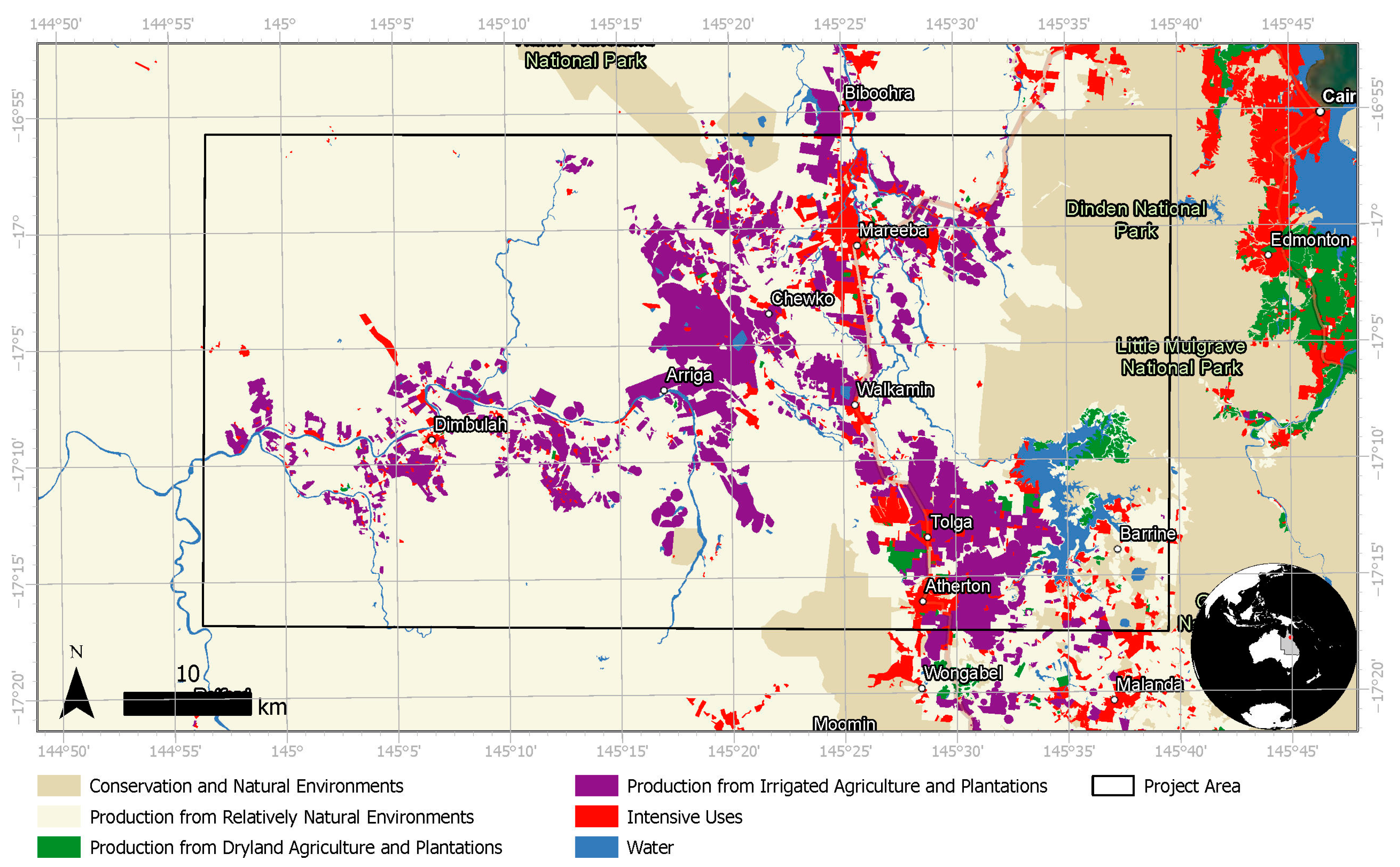
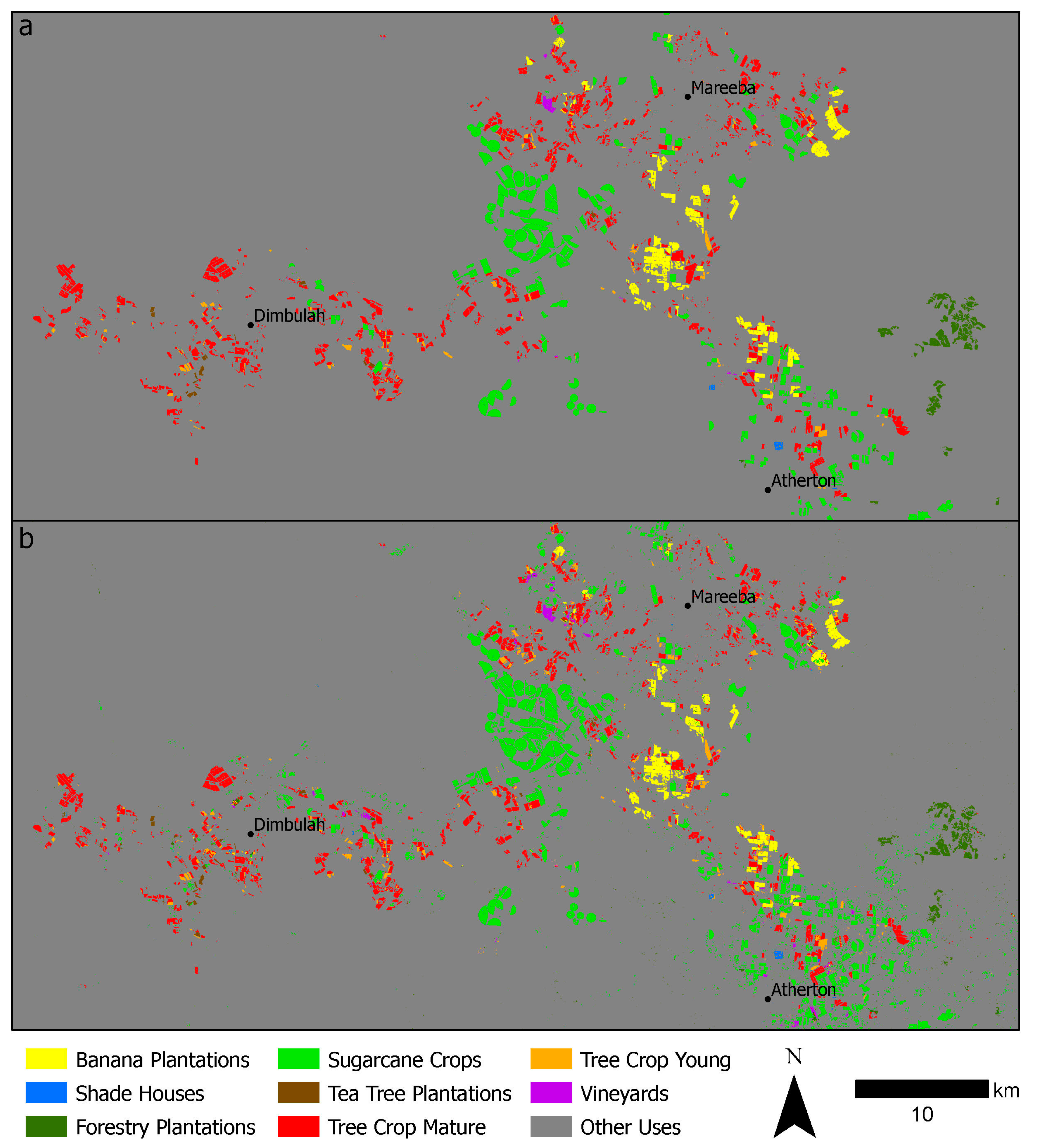
2.1. Project Area
2.2. Image Data
2.3. Data Collection
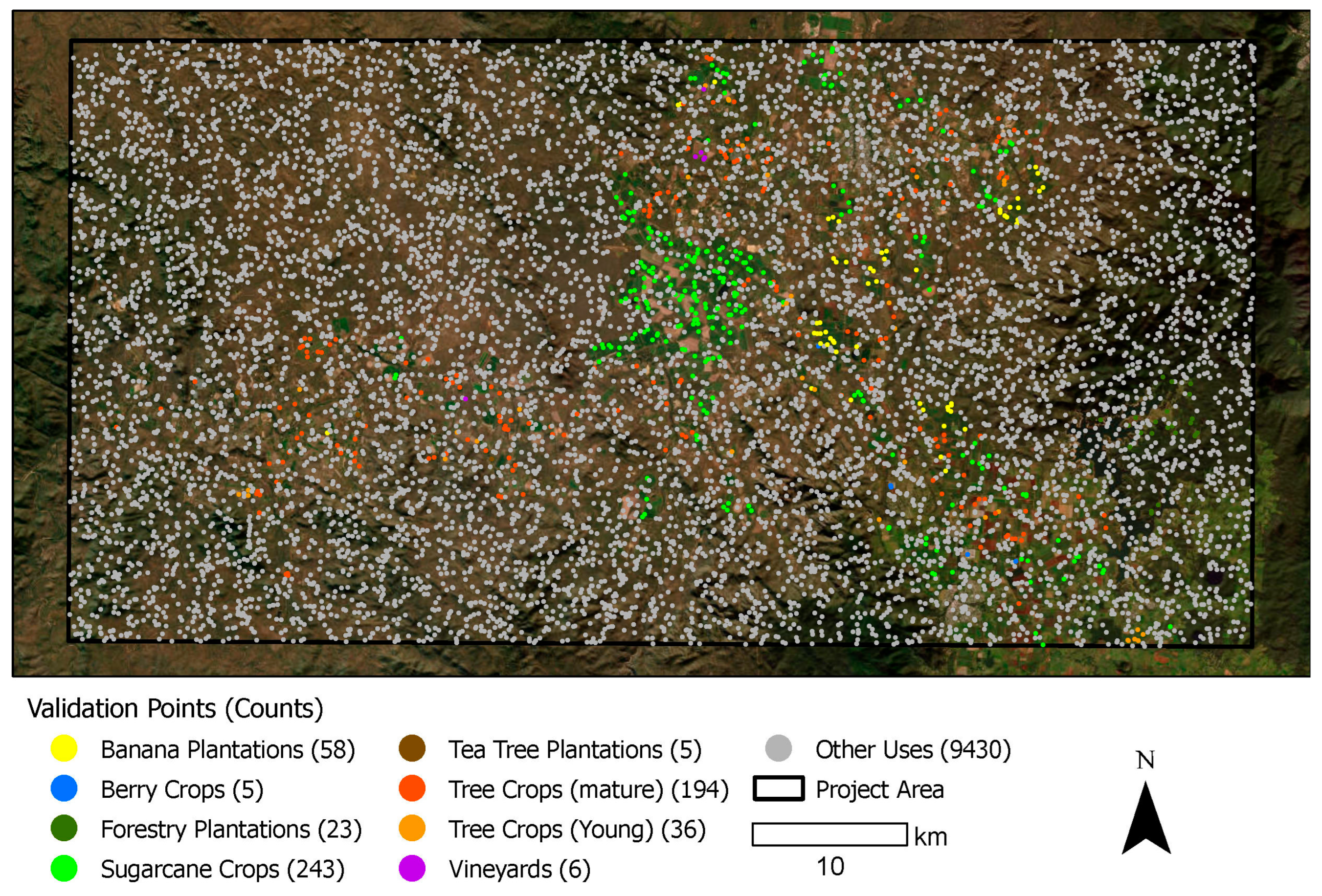
2.4. Field Verification
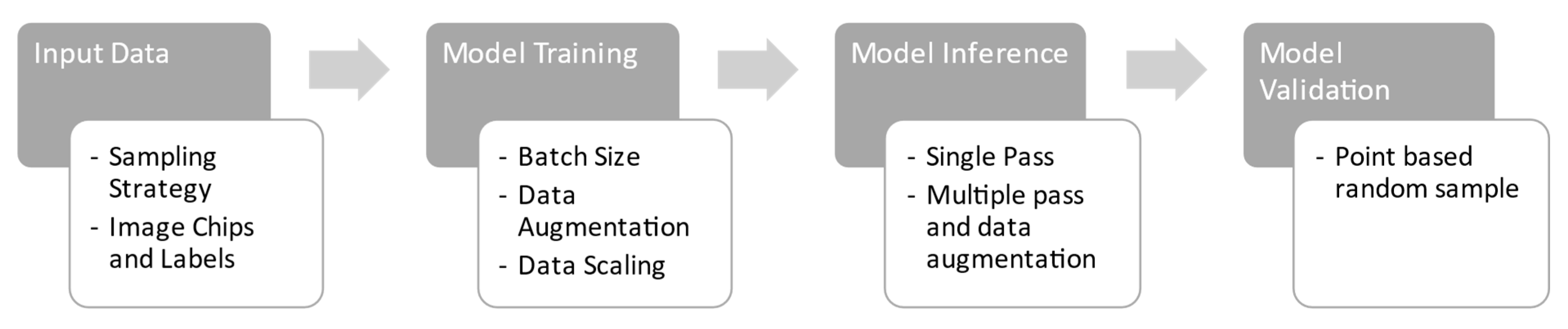
2.5. Deep Learning Trials
2.5.1. Batch Size
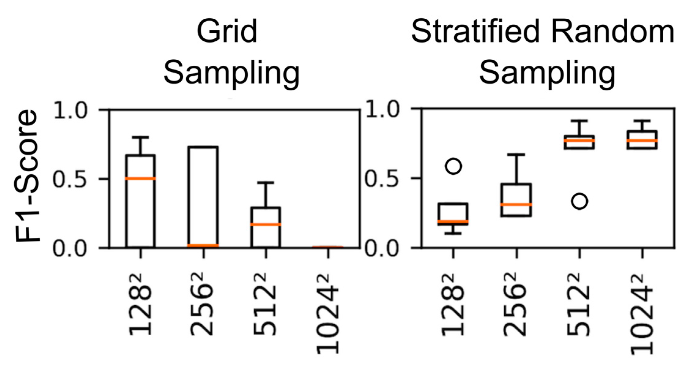
2.5.2. Patch Size and Sampling Strategy
- Grid sampling strategy
- Stratified random sampling strategy
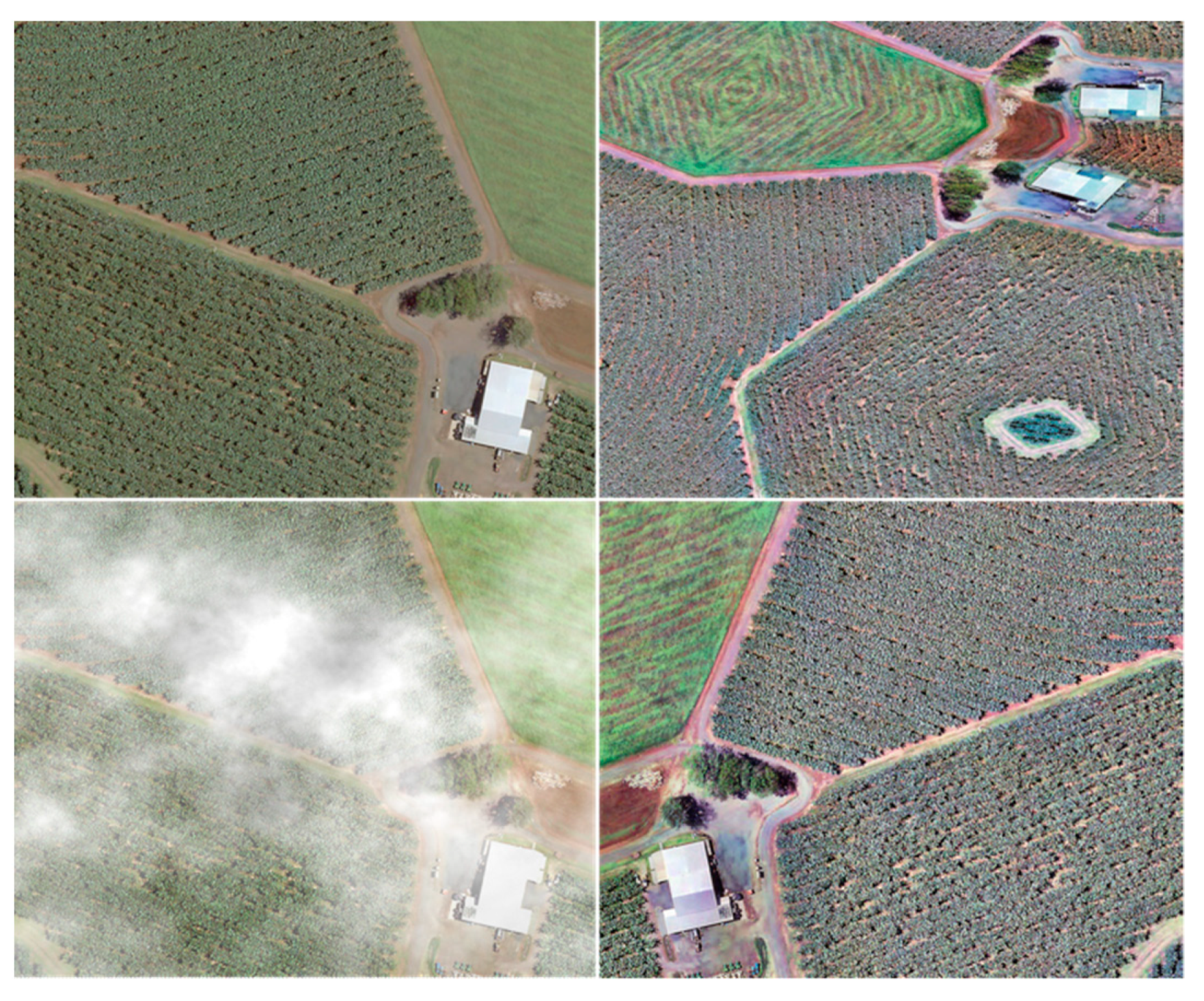
2.5.3. Data Augmentations
- altering the contrast and colourations (gamma, sigmoid, AllChannelsCLASHE, linear, multiply and allChannelsHistogramEqualization);
- adding noise to the image (salt and pepper, multiply element-wise, additive Gaussian, additive Poisson and multiply—different for each channel);
- and altering the geometry and scale of the image by zooming and stretching the image (affine, elastic transformation, vertical and horizontal flips);
- adding blur and artificial clouds/fog/smoke to mimic varying environmental and climatic conditions, different resolutions, capture angles and aircraft roll effects, which are not always fully corrected in the provided imagery.
2.5.4. Data Scaling
2.5.5. Multiple-Pass Prediction
2.5.6. Patch Image and Label Generation
2.6. Training
2.7. Prediction
2.8. Accuracy Assessment
2.9. Ranking the Trials
2.10. Full Training of Top-Performing Models
2.11. Computing Infrastructure and Software
3. Results and Discussion
3.1. Training Data
3.2. Batch Size
3.3. Patch Size and Sampling Strategy
3.4. Data Augmentation
3.5. Data Scaling
3.6. Multiple-Pass Prediction
3.7. Full Training
4. Limitations and Future Research
5. Conclusions
Author Contributions
Funding
Institutional Review Board Statement
Informed Consent Statement
Data Availability Statement
Acknowledgments
Conflicts of Interest
References
- Blaschke, T.; Hay, G.J.; Kelly, M.; Lang, S.; Hofmann, P.; Addink, E.; Queiroz Feitosa, R.; van der Meer, F.; van der Werff, H.; van Coillie, F.; et al. Geographic Object-Based Image Analysis—Towards a New Paradigm. ISPRS J. Photogramm. Remote Sens. 2014, 87, 180–191. [Google Scholar] [CrossRef] [PubMed] [Green Version]
- Hey, T.; Tansley, S.; Tolle, K.; Gray, J. The Fourth Paradigm: Data-Intensive Scientific Discovery; Microsoft Research: Redomon, WA, USA, 2009; ISBN 978-0-9825442-0-4. [Google Scholar]
- Cheng, G.; Han, J.; Guo, L.; Liu, Z.; Bu, S.; Ren, J. Effective and Efficient Midlevel Visual Elements-Oriented Land-Use Classification Using VHR Remote Sensing Images. IEEE Trans. Geosci. Remote Sens. 2015, 53, 4238–4249. [Google Scholar] [CrossRef] [Green Version]
- Ma, Y.; Wu, H.; Wang, L.; Huang, B.; Ranjan, R.; Zomaya, A.; Jie, W. Remote Sensing Big Data Computing: Challenges and Opportunities. Future Gener. Comput. Syst. 2015, 51, 47–60. [Google Scholar] [CrossRef] [Green Version]
- Bai, X.; Sharma, R.C.; Tateishi, R.; Kondoh, A.; Wuliangha, B.; Tana, G. A Detailed and High-Resolution Land Use and Land Cover Change Analysis over the Past 16 Years in the Horqin Sandy Land, Inner Mongolia. Math. Probl. Eng. 2017, 2017, 1–13. [Google Scholar] [CrossRef]
- Lillesand, T.M.; Kiefer, R.W.; Chipman, J.W. Remote Sensing and Image Interpretation, 7th ed.; John Wiley & Sons, Inc.: Hoboken, NJ, USA, 2015; ISBN 978-1-118-34328-9. [Google Scholar]
- Jensen, J.R. Remote Sensing of the Environment: An Earth Resource Perspective, 2nd ed.; Prentice Hall Series in Geographic Information Science; Pearson Prentice Hall: Upper Saddle River, NJ, USA, 2007; ISBN 978-0-13-188950-7. [Google Scholar]
- Pandey, P.C.; Koutsias, N.; Petropoulos, G.P.; Srivastava, P.K.; Dor, E.B. Land Use/Land Cover in View of Earth Observation: Data Sources, Input Dimensions, and Classifiers—A Review of the State of the Art. Geocarto Int. 2021, 36, 957–988. [Google Scholar] [CrossRef]
- Ball, J.E.; Anderson, D.T.; Chan, C.S. Comprehensive Survey of Deep Learning in Remote Sensing: Theories, Tools, and Challenges for the Community. J. Appl. Remote Sens. 2017, 11, 1. [Google Scholar] [CrossRef] [Green Version]
- Deng, L. A Tutorial Survey of Architectures, Algorithms, and Applications for Deep Learning. APSIPA Trans. Signal Inf. Process. 2014, 3, e2. [Google Scholar] [CrossRef] [Green Version]
- Ma, L.; Liu, Y.; Zhang, X.; Ye, Y.; Yin, G.; Johnson, B.A. Deep Learning in Remote Sensing Applications: A Meta-Analysis and Review. ISPRS J. Photogramm. Remote Sens. 2019, 152, 166–177. [Google Scholar] [CrossRef]
- Zhang, L.; Zhang, L.; Du, B. Deep Learning for Remote Sensing Data: A Technical Tutorial on the State of the Art. IEEE Geosci. Remote Sens. Mag. 2016, 4, 22–40. [Google Scholar] [CrossRef]
- Hoeser, T.; Kuenzer, C. Object Detection and Image Segmentation with Deep Learning on Earth Observation Data: A Review-Part I: Evolution and Recent Trends. Remote Sens. 2020, 12, 1667. [Google Scholar] [CrossRef]
- Kattenborn, T.; Leitloff, J.; Schiefer, F.; Hinz, S. Review on Convolutional Neural Networks (CNN) in Vegetation Remote Sensing. ISPRS J. Photogramm. Remote Sens. 2021, 173, 24–49. [Google Scholar] [CrossRef]
- Zang, N.; Cao, Y.; Wang, Y.; Huang, B.; Zhang, L.; Mathiopoulos, P.T. Land-Use Mapping for High-Spatial Resolution Remote Sensing Image Via Deep Learning: A Review. IEEE J. Sel. Top. Appl. Earth Obs. Remote Sens. 2021, 14, 5372–5391. [Google Scholar] [CrossRef]
- Maxwell, A.E.; Warner, T.A.; Guillén, L.A. Accuracy Assessment in Convolutional Neural Network-Based Deep Learning Remote Sensing Studies—Part 2: Recommendations and Best Practices. Remote Sens. 2021, 13, 2591. [Google Scholar] [CrossRef]
- Ronneberger, O.; Fischer, P.; Brox, T. U-Net: Convolutional Networks for Biomedical Image Segmentation. arXiv 2015, arXiv:1505.04597. [Google Scholar]
- Flood, N.; Watson, F.; Collett, L. Using a U-Net Convolutional Neural Network to Map Woody Vegetation Extent from High Resolution Satellite Imagery Across Queensland, Australia. Int. J. Appl. Earth Obs. Geoinf. 2019, 82, 101897. [Google Scholar] [CrossRef]
- Neupane, B.; Horanont, T.; Hung, N.D. Deep Learning Based Banana Plant Detection and Counting Using High-Resolution Red-Green-Blue (RGB) Images Collected from Unmanned Aerial Vehicle (UAV). PLoS ONE 2019, 14, e0223906. [Google Scholar] [CrossRef] [PubMed]
- Clark, A.; McKechnie, J. Detecting Banana Plantations in the Wet Tropics, Australia, Using Aerial Photography and U-Net. Appl. Sci. 2020, 10, 2017. [Google Scholar] [CrossRef] [Green Version]
- Burke, M.; Driscoll, A.; Lobell, D.B.; Ermon, S. Using Satellite Imagery to Understand and Promote Sustainable Development. Science 2021, 371, eabe8628. [Google Scholar] [CrossRef]
- Zhang, C.; Li, X. Land Use and Land Cover Mapping in the Era of Big Data. Land 2022, 11, 1692. [Google Scholar] [CrossRef]
- Vali, A.; Comai, S.; Matteucci, M. Deep Learning for Land Use and Land Cover Classification Based on Hyperspectral and Multispectral Earth Observation Data: A Review. Remote Sens. 2020, 12, 2495. [Google Scholar] [CrossRef]
- DSITI. Land Use Summary 1999–2015 for the Atherton Tablelands; Department of Science, Information Technology and Innovation, Queensland Government: Brisbane, Australia, 2017; p. 26.
- Dosovitskiy, A.; Springenberg, J.T.; Brox, T. Unsupervised Feature Learning by Augmenting Single Images. arXiv 2013, arXiv:1312.5242. [Google Scholar]
- Wieland, M.; Li, Y.; Martinis, S. Multi-Sensor Cloud and Cloud Shadow Segmentation with a Convolutional Neural Network. Remote Sens. Environ. 2019, 230, 111203. [Google Scholar] [CrossRef]
- Sun, Y.; Tian, Y.; Xu, Y. Problems of Encoder-Decoder Frameworks for High-Resolution Remote Sensing Image Segmentation: Structural Stereotype and Insufficient Learning. Neurocomputing 2019, 330, 297–304. [Google Scholar] [CrossRef]
- Abadi, M.; Agarwal, A.; Barham, P.; Brevdo, E.; Chen, Z.; Citro, C.; Corrado, G.S.; Davis, A.; Dean, J.; Devin, M.; et al. TensorFlow: Large-Scale Machine Learning on Heterogeneous Distributed Systems. arXiv 2016, arXiv:1603.04467. [Google Scholar]
- Qin, R.; Liu, T. A Review of Landcover Classification with Very-High Resolution Remotely Sensed Optical Images—Analysis Unit, Model Scalability and Transferability. Remote Sens. 2022, 14, 646. [Google Scholar] [CrossRef]
- Van Coillie, F.M.B.; Gardin, S.; Anseel, F.; Duyck, W.; Verbeke, L.P.C.; De Wulf, R.R. Variability of Operator Performance in Remote-Sensing Image Interpretation: The Importance of Human and External Factors. Int. J. Remote Sens. 2014, 35, 754–778. [Google Scholar] [CrossRef]
- Kandel, I.; Castelli, M. The Effect of Batch Size on the Generalizability of the Convolutional Neural Networks on a Histopathology Dataset. ICT Express 2020, 6, 312–315. [Google Scholar] [CrossRef]
- Keskar, N.S.; Mudigere, D.; Nocedal, J.; Smelyanskiy, M.; Tang, P.T.P. On Large-Batch Training for Deep Learning: Generalization Gap and Sharp Minima. arXiv 2017, arXiv:1609.04836v2. [Google Scholar]
- Caye Daudt, R.; Le Saux, B.; Boulch, A.; Gousseau, Y. Multitask Learning for Large-Scale Semantic Change Detection. Comput. Vis. Image Underst. 2019, 187, 102783. [Google Scholar] [CrossRef] [Green Version]
- Liu, S.; Qi, Z.; Li, X.; Yeh, A. Integration of Convolutional Neural Networks and Object-Based Post-Classification Refinement for Land Use and Land Cover Mapping with Optical and SAR Data. Remote Sens. 2019, 11, 690. [Google Scholar] [CrossRef] [Green Version]
- Wurm, M.; Stark, T.; Zhu, X.X.; Weigand, M.; Taubenböck, H. Semantic Segmentation of Slums in Satellite Images Using Transfer Learning on Fully Convolutional Neural Networks. ISPRS J. Photogramm. Remote Sens. 2019, 150, 59–69. [Google Scholar] [CrossRef]
- Stoian, A.; Poulain, V.; Inglada, J.; Poughon, V.; Derksen, D. Land Cover Maps Production with High Resolution Satellite Image Time Series and Convolutional Neural Networks: Adaptations and Limits for Operational Systems. Remote Sens. 2019, 11, 1986. [Google Scholar] [CrossRef] [Green Version]


| Primary Land Use | Hectares | Proportion |
|---|---|---|
| Production from relatively natural environments | 201,625 | 67.3% |
| Conservation and natural environments | 40,404 | 13.5% |
| Production from irrigated agriculture and plantations | 37,939 | 12.7% |
| Intensive uses | 10,133 | 3.4% |
| Water | 7219 | 2.4% |
| Production from dryland agriculture and plantations | 2143 | 0.7% |
| Total | 299,463 | 100.0% |
| Parameter | Number of Training Patches | Test Values | Default |
|---|---|---|---|
| Batch size | 3986 | 10, 50, 100, 150, 200, 250 and 280 | * |
| Patch size and sampling strategy | 2408–154,514 | 1282, 2562, 5122 and 10242 | 5122 |
| Data Augmentations | 22,830 | True, False | False |
| Data Scaling | 22,830 | True, False | False |
| Multiple-Pass Prediction | 22,830 | True, False | False |
| Patch Size (Pixels) | Number of Patches | Difference | Difference (%) | |
|---|---|---|---|---|
| Stratified Method | Grid Method | |||
| 128 × 128 | 154,514 | 154,112 | 402 | 0.26% |
| 256 × 256 | 38,533 | 38,528 | 5 | 0.01% |
| 512 × 512 | 9635 | 9632 | 3 | 0.03% |
| 1024 × 1024 | 2412 | 2408 | 4 | 0.17% |
| Class | 128 × 128 Pixels | 256 × 256 Pixels | 512 × 512 Pixels | 1024 × 1024 Pixels | ||||
|---|---|---|---|---|---|---|---|---|
| Grid | Stratified | Grid | Stratified | Grid | Stratified | Grid | Stratified | |
| Banana Plantations | 6155 | 17,509 | 1861 | 4535 | 637 | 1214 | 249 | 369 |
| Berry Crops | 387 | 14,050 | 129 | 3567 | 49 | 892 | 21 | 230 |
| Other | 132,194 | 98,019 | 35,955 | 3567 | 9519 | 892 | 2408 | 2410 |
| Plantation Forestry | 3604 | 16,565 | 1100 | 4191 | 360 | 1050 | 133 | 266 |
| Sugarcane Crops | 23,705 | 19,585 | 6994 | 5162 | 2247 | 1503 | 795 | 473 |
| Tea Tree | 766 | 14,795 | 274 | 3761 | 110 | 964 | 50 | 247 |
| Tree Crops—Mature | 26,360 | 24,152 | 9005 | 7151 | 3414 | 2531 | 1418 | 941 |
| Tree Crops—Young | 4361 | 17,304 | 1634 | 4636 | 722 | 1423 | 367 | 451 |
| Vineyards | 546 | 14,539 | 194 | 3693 | 84 | 933 | 43 | 241 |
| Total | 154,112 | 154,514 | 38,528 | 38,533 | 9632 | 9635 | 2408 | 2412 |
| Size (Pixels) | Number of Patches | Batch Size | Batches Per Epoch |
|---|---|---|---|
| 1024 × 1024 | 2408 | 16 | 151 |
| 512 × 512 | 9632 | 64 | 151 |
| 256 × 256 | 38,528 | 256 | 151 |
| 128 × 128 | 154,112 | 1024 | 151 |
| Trial | Parameter | Average Training Time (h) | Kappa (95% CI) | Average F1—Score (95% CI) | Average User’s Accuracy (Precision) | Average Producer’s Accuracy (Recall) | Ranking |
|---|---|---|---|---|---|---|---|
| Human Derived | Manual | >200 | 0.96 | 0.95 | 0.97 | 0.92 | - |
| Batch Size | 10 | 1.2 | 0.67 (0.62–0.71) | 0.68 (0.56–0.74) | 0.63 (0.5–0.71) | 0.84 (0.66–0.92) | 5 |
| 50 | 0.8 | 0.63 (0.62–0.65) | 0.62 (0.6–0.64) | 0.53 (0.51–0.55) | 0.91 (0.89–0.92) | 2 | |
| 100 | 0.8 | 0.55 (0.48–0.62) | 0.56 (0.54–0.59) | 0.49 (0.46–0.53) | 0.85 (0.81–0.89) | 1 | |
| 150 | 0.8 | 0.43 (0.31–0.49) | 0.51 (0.44–0.56) | 0.43 (0.38–0.49) | 0.83 (0.81–0.86) | 5 | |
| 200 | 0.8 | 0.41 (0.33–0.49) | 0.45 (0.41–0.49) | 0.38 (0.34–0.41) | 0.82 (0.81–0.83) | 4 | |
| 250 | 0.7 | 0.45 (0.33–0.51) | 0.48 (0.43–0.51) | 0.42 (0.37–0.44) | 0.79 (0.77–0.8) | 2 | |
| 280 | 0.7 | 0.36 (0.19–0.46) | 0.41 (0.31–0.45) | 0.36 (0.29–0.4) | 0.75 (0.65–0.82) | 5 | |
| Patch Size (Systematic) | 128 × 128 | 3.7 | 0.69 (0.65–0.77) | 0.49 (0.37–0.59) | 0.53 (0.35–0.66) | 0.51 (0.42–0.62) | 2 |
| 256 × 256 | 1.3 | 0.58 (0.4–0.72) | 0.48 (0.34–0.56) | 0.49 (0.34–0.61) | 0.55 (0.42–0.63) | 2 | |
| 512 × 512 | 1.2 | 0.7 (0.62–0.74) | 0.49 (0.45–0.52) | 0.53 (0.46–0.61) | 0.53 (0.46–0.61) | 1 | |
| 1024 × 1024 | 1.3 | 0.66 (0.48–0.75) | 0.42 (0.41–0.45) | 0.43 (0.4–0.46) | 0.47 (0.42–0.52) | 4 | |
| Patch Size (stratified-random) | 128 × 128 | 3.7 | 0.42 (0.38–0.49) | 0.46 (0.41–0.5) | 0.38 (0.35–0.43) | 0.86 (0.85–0.87) | 4 |
| 256 × 256 | 1.2 | 0.51 (0.47–0.58) | 0.51 (0.47–0.57) | 0.43 (0.4–0.49) | 0.86 (0.85–0.86) | 2 | |
| 512 × 512 | 1.2 | 0.65 (0.59–0.71) | 0.62 (0.52–0.67) | 0.59 (0.48–0.68) | 0.77 (0.7–0.81) | 1 | |
| 1024 × 1024 | 1.3 | 0.53 (0.31–0.66) | 0.54 (0.38–0.62) | 0.5 (0.36–0.56) | 0.71 (0.52–0.82) | 3 | |
| Data Augmentation | FALSE | 2.8 | 0.73 (0.7–0.77) | 0.7 (0.66–0.74) | 0.64 (0.58–0.68) | 0.87 (0.83–0.9) | 1 |
| TRUE | 8.9 | 0.49 (0.34–0.59) | 0.5 (0.48–0.53) | 0.43 (0.4–0.46) | 0.75 (0.72–0.77) | 2 | |
| Data Scaling | FALSE | 2.1 | 0.69 (0.62–0.74) | 0.64 (0.56–0.69) | 0.59 (0.48–0.66) | 0.78 (0.72–0.81) | 2 |
| TRUE | 2.1 | 0.77 (0.7–0.79) | 0.74 (0.68–0.78) | 0.68 (0.6–0.74) | 0.88 (0.83–0.91) | 1 | |
| Multiple-Pass Prediction | Single | 8.9 | 0.49 (0.34–0.59) | 0.5 (0.48–0.53) | 0.43 (0.4–0.46) | 0.75 (0.72–0.77) | 2 |
| Multiple | 8.9 | 0.55 (0.4–0.65) | 0.52 (0.48–0.53) | 0.45 (0.41–0.48) | 0.75 (0.69–0.81) | 1 |
| Name | Feature Count | Area (ha) | Area (%) |
|---|---|---|---|
| Banana Plantation | 243 | 1860 | 0.62 |
| Berry Crops | 69 | 92 | 0.03 |
| Forestry Plantation | 118 | 981 | 0.33 |
| Sugarcane Crop | 515 | 7621 | 2.54 |
| Tea Tree Plantation | 42 | 188 | 0.06 |
| Tree Crop—Mature | 2289 | 6249 | 2.09 |
| Tree Crop—Young | 280 | 988 | 0.33 |
| Vineyards | 33 | 146 | 0.05 |
| Other | 323 | 281,344 | 93.95 |
| Total | 3912 | 299,471 | 100.00 |
| 2018 | 2015 | |||||
|---|---|---|---|---|---|---|
| Class | F1-Score | User’s (Precision) | Producer’s (Recall) | F1-Score | User’s (Precision) | Producer’s (Recall) |
| Banana Plantations | 1.0000 | 1.0000 | 1.0000 | 0.9908 | 0.9818 | 1.0000 |
| Berry Crops | 1.0000 | 1.0000 | 1.0000 | 0.8571 | 1.0000 | 0.7500 |
| Plantation Forestry | 0.8400 | 0.9545 | 0.7500 | 0.8780 | 1.0000 | 0.7826 |
| Sugarcane Crops | 0.9839 | 1.0000 | 0.9683 | 0.9204 | 0.9946 | 0.8565 |
| Tea Tree Plantation | 1.0000 | 1.0000 | 1.0000 | 1.0000 | 1.0000 | 1.0000 |
| Tree Crop—Mature | 0.9602 | 0.9361 | 0.9856 | 0.9403 | 0.9141 | 0.9679 |
| Tree Crop—Young | 0.7297 | 0.8710 | 0.6279 | 0.6897 | 0.8696 | 0.5714 |
| Vineyards | 1.0000 | 1.0000 | 1.0000 | 1.0000 | 1.0000 | 1.0000 |
| Other | 0.9981 | 0.9973 | 0.9989 | 0.9968 | 0.9950 | 0.9987 |
| Total | 0.9458 | 0.9732 | 0.9256 | 0.9192 | 0.9728 | 0.8808 |
| Kappa | 0.9617 | 0.9293 | ||||
| Parameter | Average Training Time (h) | Kappa (95% CI) | Average F1-Score (95% CI) | Average User’s Accuracy (Precision) | Average Producer’s Accuracy (Recall) | Ranking |
|---|---|---|---|---|---|---|
| False | 2.8 | 0.12 (0.09–0.15) | 0.21 (0.18–0.25) | 0.22 (0.18–0.27) | 0.35 (0.31–0.39) | 2 |
| True | 8.9 | 0.36 (0.27–0.41) | 0.4 (0.38–0.41) | 0.37 (0.33–0.4) | 0.61 (0.57–0.65) | 1 |
| Parameter | Value |
|---|---|
| Patch size (pixels) | 512 × 512 |
| Sampling strategy | Stratified random sample (area) |
| Number of patches | 22,830 |
| Batch size | 20 |
| Data Augmentations | True |
| Data Scaling | True |
| Multiple-Pass Prediction | True |
| Image | Kappa (95% CI) | Average F1-Score (95% CI) | Average User’s (95% CI) (Precision) | Average Producer’s (95% CI) (Recall) |
|---|---|---|---|---|
| 2018 | 0.9 (0.89–0.91) | 0.87 (0.86–0.89) | 0.8 (0.78–0.83) | 0.98 (0.98–0.98) |
| 2015 | 0.84 (0.82–0.87) | 0.81 (0.79–0.84) | 0.78 (0.76–0.8) | 0.87 (0.85–0.9) |
Disclaimer/Publisher’s Note: The statements, opinions and data contained in all publications are solely those of the individual author(s) and contributor(s) and not of MDPI and/or the editor(s). MDPI and/or the editor(s) disclaim responsibility for any injury to people or property resulting from any ideas, methods, instructions or products referred to in the content. |
© 2023 by the authors. Licensee MDPI, Basel, Switzerland. This article is an open access article distributed under the terms and conditions of the Creative Commons Attribution (CC BY) license (https://creativecommons.org/licenses/by/4.0/).
Share and Cite
Clark, A.; Phinn, S.; Scarth, P. Pre-Processing Training Data Improves Accuracy and Generalisability of Convolutional Neural Network Based Landscape Semantic Segmentation. Land 2023, 12, 1268. https://doi.org/10.3390/land12071268
Clark A, Phinn S, Scarth P. Pre-Processing Training Data Improves Accuracy and Generalisability of Convolutional Neural Network Based Landscape Semantic Segmentation. Land. 2023; 12(7):1268. https://doi.org/10.3390/land12071268
Chicago/Turabian StyleClark, Andrew, Stuart Phinn, and Peter Scarth. 2023. "Pre-Processing Training Data Improves Accuracy and Generalisability of Convolutional Neural Network Based Landscape Semantic Segmentation" Land 12, no. 7: 1268. https://doi.org/10.3390/land12071268
APA StyleClark, A., Phinn, S., & Scarth, P. (2023). Pre-Processing Training Data Improves Accuracy and Generalisability of Convolutional Neural Network Based Landscape Semantic Segmentation. Land, 12(7), 1268. https://doi.org/10.3390/land12071268