Article

“Location, Location, Location”: Fluctuations in Real Estate Market Values after COVID-19 and the War in Ukraine Based on Econometric and Spatial Analysis, Random Forest, and Multivariate Regression

by
Laura Gabrielli
*,
Aurora Greta Ruggeri
and
Massimiliano Scarpa
Department of Architecture and Arts, University IUAV of Venice, Dorsoduro 2206, 30123 Venice, Italy
*
Author to whom correspondence should be addressed.
Land 2023, 12(6), 1248; https://doi.org/10.3390/land12061248
Submission received: 15 May 2023 / Revised: 12 June 2023 / Accepted: 16 June 2023 / Published: 19 June 2023
(This article belongs to the Special Issue Landscapes at Risk. Social Capital Asset in the COVID-Scape Climate)

Abstract

:
In this research, the authors aim to detect the marginal appreciation of construction and neighbourhood characteristics of property prices at three different time points: before the COVID-19 pandemic, two years after the first COVID-19 alert but before the War in Ukraine, and one year after the outbreak of the War. The marginal appreciations of the building’s features are analysed for a pilot case study in Northern Italy using a Random Forest feature importance analysis and a Multivariate Regression. Several techniques are integrated into this study, such as computer programming in Python language, multi-parametric value assessment techniques, feature selection procedures, and spatial analysis. The results may represent an interesting ongoing monitoring of how these anomalous events affect the buyer’s willingness to pay for specific characteristics of the buildings, with particular attention to the location features of the neighbourhood and accessibility.

1. Introduction

1.1. Fixed Effects and Market Value

“There are three things that matter in property: location, location, location”, states Lord Harold Samuel in his iconic sentence [1]. Even though the location is not the only characteristic of a property on which its market value depends, it is undoubtedly one of the most significant features, if not the most important one. As such, this research will discuss how fixed effects influence the best estimate of a property’s market value through multi-parametric estimation techniques [2,3]. Concomitantly, the authors wish to investigate whether the recent events of the COVID-19 pandemic and the War in Ukraine have changed the influence of a property’s location on its market value.
Has a demand shift occurred due to these impactful and significant events? Does the axiom “location, location, location” still remains unchanged?
This investigation is carried out from a market value perspective. The aim is to analyse whether the factors contributing to price formation have changed, questioning whether the demand has altered the appreciation of certain building features over time or if some of the usually most significant factors have become less influential in assessing the market values. The approach proposed is strongly interdisciplinary, integrating statistical techniques with economic analyses and geographic-spatial information. The intersection between statistics, economics, regional science, and econometrics can be identified as spatial econometrics or spatial analysis, which is sometimes (improperly) used as synonyms [4]. This research field helps to understand the spatial aspect of economic events, analyse spatial relationships, and leads to the production of a geographically centred interpretation of observations.
Specifically, this paper will apply a multivariate regression (MR) with spatial regressors to an illustrative case study to assess a property’s market value as a function of its descriptive features, such as location, distance from specific points of interest, construction features, and size. The MR will be developed based on three databases collected at different time points but pertaining to the same city (i.e., Padova, Northern Italy). The first database represents a pre-COVID-19 scenario. The second database was collected two years after the first COVID-19 alert, therefore illustrating the first effects that the pandemic has brought to the real estate market in North Italy. In contrast, the third database was collected one year after the outbreak of the War in Ukraine.
The MR belongs to multi-parametric market value assessment techniques. Such methodologies are extremely useful for the present work since they assess a property market value depending on a bundle of its descriptive characteristics. While in mono-parametric approaches, the estimate of the market value is only described as a function of one single characteristic of the building, most commonly the floor area (sqm); multi-parametric methods are able to include and balance a plethora of descriptive information of a property, comprising both construction and neighbourhood features [5].
Among the neighbourhood characteristics, the authors’ intent is to analyse the location of the building in central, semi-central, or suburban areas, its proximity to the city centre and public services, the accessibility to public transport or employment centres, but also the urban quality of the district, including pollution, healthy environment, parks and gardens, social context and security, leisure services, absence of high noises, or low building density.
As far as construction characteristics are concerned, it is the author’s will to consider simultaneously several features that define the quality of the building, such as its size, the number of rooms and bathrooms, the floor level, the maintenance status, the quality of materials, the energy performance, the presence of technologies such as domotics, photovoltaic systems or solar panels, the presence of additional areas such as a balcony, a private garden, or a garage, and the orientation of the building or its panorama and view.

1.2. Choosing the Econometric Model among the Multi-Parametric Value Assessment Methods

In the field of property valuation in Italy, multi-parametric methods include the simplified scoring techniques called “punti di merito” (in its two variants, i.e., the “additive approach” or the “multiplicative approach”), the “market comparison approach”, a method originated in the United States and reinterpreted in our country [6,7,8], and the “econometric models” or the more sophisticated “machine learning” models [9].
Econometric and machine learning models can be used as a mass appraisal technique in real estate valuation. A mass appraisal technique can be defined as the process of valuing a building stock or a property asset based on common parameters and statistical techniques [10].
The latter two methodologies, in general, aim to find the statistical relationship/algorithm that relates some economic quantities describing the property (independent variables) and the market value (dependent variable) [11].
The econometric model of hedonic prices quantifies how much each independent variable contributes to the variation of the market price. Each variable is assigned a numerical coefficient, and a mathematical assessment formula is consequently built [12]. Machine learning assessment procedures, such as Regression Trees and Random Forest, Artificial Neural Networks, Nearest Neighbours, Support Vector Machines, and Genetic Algorithms, ensure great accuracy in the value assessment. They enable the inclusion of numerous independent variables in the predictive model and can produce complex forecasting algorithms [13,14].
Econometric approaches generally have a high inferential capacity at the expense of a lower predictive capacity [15,16], while machine learning procedures show a higher predictive capacity but a lower inferential capacity [17,18]. Since inferential capacity refers to the effectiveness of the model in identifying cause–effect relationships among dependent and independent variables, whereas the predictive capacity represents the ability of the model to produce forecasts really close to the expected values, the authors believe that for the purposes of this article, the hedonic price estimation method could be the best choice to investigate the fixed effects in the real estate market.
The hedonic price method is founded on the assumption that a property is characterised by a set of elements (the building characteristics) and that the value of the property can be calculated as a sum of the estimated values of its elements [19]. This way, a marginal price is given to every building attribute, implicitly understanding how much that characteristic influences the market value [20]. In any real estate market, the demand compares the buildings for sale based on their characteristics, and the buyer will purchase the property that seems the most convenient. However, different characteristics are valued differently by the operators on the demand side. Some characteristics may be considered almost “objectively” valued by the demand, while others remain highly subjective. The marginal prices of the building characteristics depend on several factors, such as the housing market segment, politics and laws, fashions and trends, market cycles, social status, and the spending capacity of the demand, and they are subject to variation over time.
As such, the paper is structured as follows. Section 2 will introduce the methodological approach adopted for this research, while Section 3 describes the practical case study. A discussion about the regressors is illustrated in Section 4, whereas Section 5 outlines the complex procedure involved in downloading information, and Section 6 presents the Random Forest feature importance process. In Section 7, the Multivariate Regressions and the spatial analyses are developed and discussed. Finally, Section 8 draws the conclusions of this research, highlighting further possible developments.

2. Purpose and Materials and Methods

2.1. A Diachronic Analysis Related to Major Anomalous Events

As the authors are leading this research, it is early 2023. The present study is a specific development of a more comprehensive research stream that monitors and investigates multi-parametric value assessment techniques and hedonic prices in several Italian markets over time [21,22]. As a result of the globally impactful events that have occurred in recent years, this monitoring process of real estate values and marginal prices allows us to describe the shifts in demand preferences after the COVID-19 diffusion and the outbreak of War in Ukraine.
As of now, more than three years have elapsed since the first signs of the pandemic emerged in December 2019, originating from China [23], leading to various effects on the economy, labour, or trade, other than its clear impact on the health sector [24]. On the other hand, more than a year has passed since the outbreak of the War in Ukraine, when in the early morning of 24 February 2022, Russia launched numerous attacks on Ukraine’s major cities [25]. The domino effect of this unfortunate event changes the dynamics of so many sectors, directly and indirectly, bringing obvious consequences, such as political, financial [26,27,28], environmental, and energy-related impacts [29,30,31]. Further, it has also affected psychological health and social dynamics [32,33,34]. Moreover, these significant events also impact the real estate sector in terms of demand preferences, cost of construction, willingness to pay, property prices, and market dynamics.
Regarding our field of interest, real estate Researchers and Professionals are now wondering how and to what extent both the COVID-19 pandemic [35,36,37,38] and the War in Ukraine [39,40] might affect price formation mechanisms and thus their profession.
The scope of this research is twofold. On the one hand, the aim is to understand the marginal contribution of building features to the price, distinguishing between the fixed effects (location, neighbourhood, and accessibility) and the building’s construction characteristics. On the other hand, the analysis is diachronic, aiming to point out if any difference in the marginal appreciation of the features has occurred due to COVID-19 and the War in Ukraine.
Political, geographical, social, and economic factors strongly influence real estate market dynamics. In this case, those factors can undoubtedly be classified as anomalous events. Well defined in [41], an anomalous event is an unexpected and unpredicted shock whose causes are exogenous to the market in question, but the effects change and influence the market. The methods applied and the intended purposes in the research that have analysed the effect of anomalous events on the housing market appear to be very heterogeneous, primarily differing on the basis of the extent of the impact, i.e., distinguishing events with microeconomic consequences from events with macroeconomic consequences, as is the case in this study. Another distinction that should be considered is temporary versus permanent effects on the market dynamics.
The methodologies employed on an international panorama to analyse such anomalous phenomena are varied and multifaceted, showing different approaches and scopes. For instance, in [42], the authors conducted an economic analysis of the historical series in the United States over a 90-year time span and related natural disasters to economic responses. The hedonic price approach is widely employed in the literature to relate anomalous events and price changes. Several techniques have also been employed in the literature to understand the marginal contribution that building features (construction and neighbourhood) bring to the formation of the market price, such as spatial analysis, GIS (geographic information system), and, again, hedonic price regressions and neural networks [43,44].

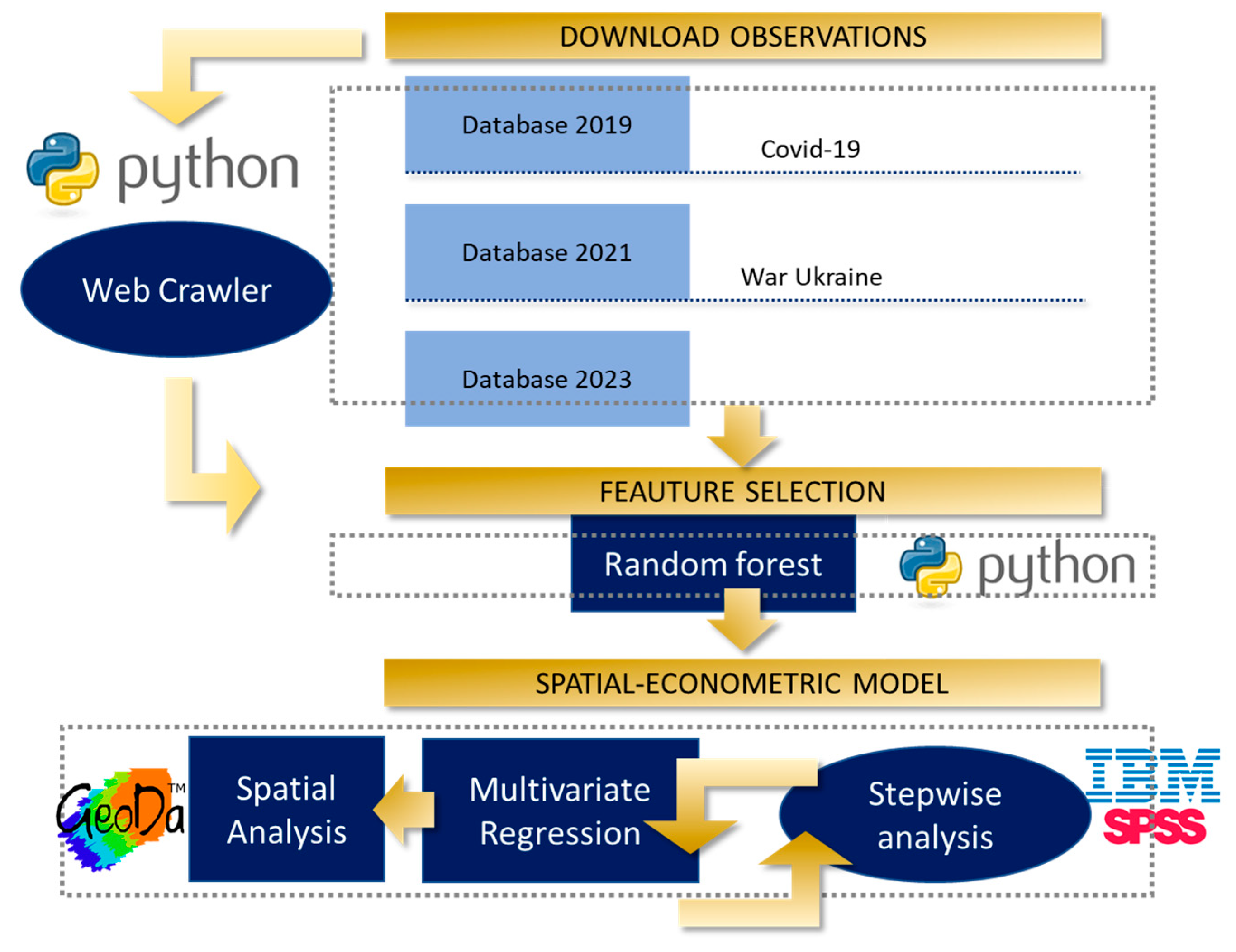
2.2. Methodological Approach and Workflow

For this research, as introduced in Section 1, the hedonic price approach is adopted through an optimized and multivariate polynomial regression. The methodological strategy leading to understanding the price formation mechanisms after the COVID-19 pandemic and the War in Ukraine, illustrated in Figure 1, is as follows:
  • In STEP 1, the exemplary case study is defined, i.e., the real estate market in Padova. The case study is described based on three databases (DBs) collected at different times. The first database is dated 2019, II semester, representing the pre-COVID-19 situation. It is named DB2019 for the sake of simplicity. The second database is dated 2021, II semester, portraying the market two years after the first COVID-19 alert but before the outbreak of the War. It is called DB2021. The third database is dated 2023, I semester, depicting the market changes one year after the outbreak of the War in Ukraine. This last database is named DB2023.
  • As far as STEP 2 is concerned, a set of construction and neighbourhood descriptive features of the buildings are selected and discussed as the independent regressors in the econometric models. In contrast, the market value of the property is the dependent variable.
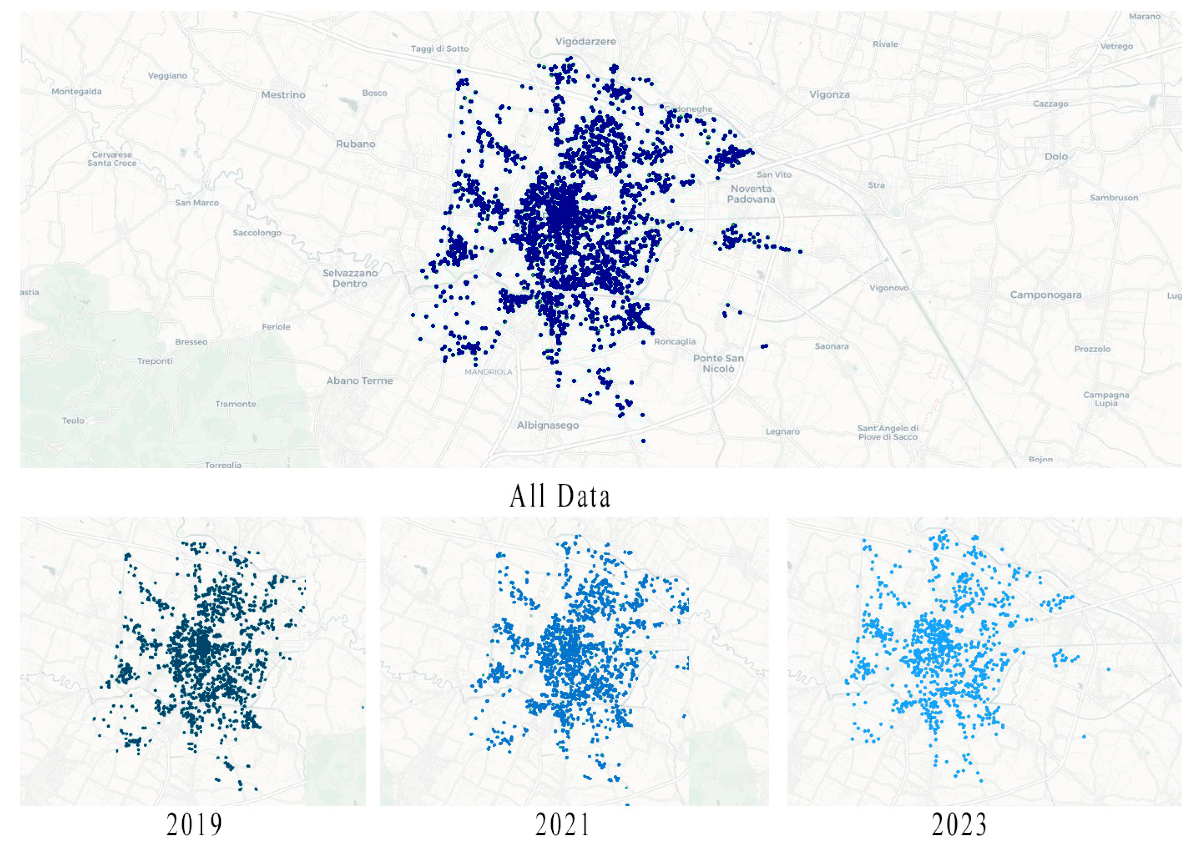
  • In STEP 3, the authors develop an automated procedure to download data and information about the buildings for sale in Padova. This step is carried out in Python® computer language, producing a web-crawling software to browse and extract information from web pages according to a predefined path. The web crawler has been used three times (2019, II semester; 2021, II semester; 2023, I semester) to read and download information from specific Italian selling websites regarding properties for sale, monitoring market changes in asking prices over time.
  • Before producing the regression models, in STEP 4, a feature selection process is conducted to understand how each predictor variable influences the response variable and eliminate the less significant regressors. The feature selection procedure helps to simplify the model outcome, reduces computational time, and overcomes the overfitting problem. The Random Forest (RF) regressor is used to test the variable importance, leading to exclude some predictors from the regression models. The RF procedure is again conducted in Python code.
  • STEP 5 produces the spatial-econometric models as Multivariate Regressions (MRs). The econometric model MR2019 is developed based on the dataset DB2019, the MR2021 refers to the dataset DB2019, and the MR2023 corresponds to DB2023. The spatial analyses are conducted using the GeoDa® software, while the stepwise analysis produced to define the MRs is developed with the help of the IBM SPSS 29® software.

3. The Case Study

Since the authors have been monitoring and recording data about the city of Padova during the last years to carry out several research projects, this may represent a good case study to understand market variations over time after the latest events because of the enormous data availability about this city. Nevertheless, this case study can also be a good representative of market changes because, besides the access to high-quality and numerous information, Italy is one of the countries majorly hit by COVID-19 and its economic consequences.
Indirect sources (aggregated market quotations) show that after a steep decrease, medium asking prices increased slightly again after the pandemic’s beginning. Moreover, this increment keeps constant in 2019–2023, as represented in Figure 2 [45]. Those data have been collected from historical web archives regarding residential properties on sale (asking prices) considering, at an aggregate level, excellent, good, and poor conditions.
Other sources of indirect information, namely, the Nomisma publications [46] and also the real estate Observatory “OMI” (Osservatorio Mercato Immobiliare) [47], provide the historical series of the actual transaction prices. The difference between the asking prices and the market values (real transactions) gives an idea of the medium negotiation margin. Figure 3 displays the selling prices recorded in Padova from the Nomisma Market Observatory from 2010 to 2022 (the latest information available), while Table 1 resumes data from 2019 to 2022. In this case, the transaction prices have kept relatively constant since 2019, with a slight increase beginning in 2022. In fact, there is always a time lag in the response of transaction prices if compared to the concomitant increase/decrease in the asking prices. Regarding the margin of negotiation, it is now around 4.5% for new constructions and 8.5% for residential properties to be refurbished. The time required to sell a property is around 4.8 months for properties in excellent maintenance and 5 months for good and poor conditions [46].
From 2019 to 2023, the negotiation margin decreased by 3.5% for old buildings and 2% for new constructions. Moreover, the time required to sell a property has decreased from 2019 to 2023, diminishing by 1.7 months for old constructions and 1.3 months for new buildings [46].

4. A Discussion of Construction and Neighbourhood Variables

This chapter aims to define and discuss the descriptive independent variables of each building collected over time to define DB2019, DB2021, and DB2023. The independent variables will be the regressors, expressing their contribution to the price formation in the MR, and the dependent variable will therefore be the property’s market value. As introduced in Section 1, the hedonic price method explicitly refers to the principle that the market value of a building depends on a bundle of its characteristics [19]. For this research, the characteristics of the building that determine its price are generally classified into construction and neighbourhood. This distinction allows us to check whether the neighbourhood features vary in their contribution to the price formation over time.

4.1. Construction Parameters

Regarding construction features, they represent a property’s physical features and are directly related to the building typology [48]. Construction features are otherwise indicated as dwelling or building characteristics.
According to [49], construction characteristics may be logically clustered into two complementary sub-groups, i.e., the single dwelling and building characteristics. On the one hand, the first bundle of features strictly refers to the single dwelling and describes the peculiarities of each unit located in a building, including physical features (such as the floor area, the number of rooms, the number of bathrooms, and the maintenance conditions) and technological features (including heating/cooling systems, solar or photovoltaics panels, domotics, alarm systems, or others).
On the other hand, the building characteristics describe the features of the entire building shared by all the single units, such as the presence of a shared garden, parking spaces, lifts, or shared terraces. Clearly, for single-building typologies and independent constructions, the two sub-groups coincide.
In this research, the construction features of the premises are resumed by a total of 40 indicators that are displayed in Table 2.

4.2. Neighbourhood Parameters

For what concerns the neighbourhood characteristics, instead, they represent the location of the building, and they describe its external environment and position. Therefore, the neighbourhood characteristics are chosen to conduct a spatial-econometric analysis, where the economic value of the building is assessed as a function of its location attributes. As defined in [50], spatial analysis generates helpful knowledge to answer questions about order, pattern, and structure inherent in spatial problems. Therefore, the MR’s quantitative methodology is intended to answer a spatial question to understand market value fluctuations along a diachronic analysis in relation to position and neighbourhood.
Neighbourhood features may be classified into two groups: urban attributes and accessibility attributes.
On the one hand, urban attributes are related to the level of urban quality. As it goes without saying, a buyer would be willing to pay a higher price for a property located in a position with higher urban quality. Even though no specific literature provides an exhaustive list of the urban attributes (otherwise called urban amenities) that fully describe what drives the buyer’s choice, the classification proposed in [51] is often adopted in these kinds of research. The authors [51] classify urban amenities into natural amenities, such as air quality, water presence, and open spaces; historical amenities, such as monuments, historical sites, or cultural infrastructures; and modern amenities, for example, hospitals and health services, shopping malls, educational buildings, leisure, banks, or others. Another classification for the urban characteristics may divide supply services from open-air amenities. Among the supply services, there are all medical and health facilities (hospital and medical care centres, pharmacies, and herbalists), financial facilities (banks and postal services), educational facilities (nurseries, kindergartens, elementary schools, middle schools, high schools, and universities), cultural facilities (theatres, cinemas, libraries, galleries, museums, and opera houses), commercial facilities (shopping centres, malls, supermarkets, groceries, and tobacconists), and sports facilities (fitness, pools, and sports centres). The open-air amenities are public parks and gardens, playgrounds, walking areas, natural paths, cycle lanes, skating areas, rugby/football/volleyball/basketball/tennis courts, or open-air swimming pools.
On the other hand, accessibility attributes are related to the distance of the house from specific points of interest (POI), such as the city centre, and the link to transportation systems, such as train stations, subway stations, accesses to motorways and ring roads, but also to bus stops and trams.
In this research, urban attributes and accessibility are characterised by analysing the following POI: city centre, train station, bus stop and tram stop, education facilities, big shopping malls, big commercial facilities, small supermarkets, urban parks/public gardens, sports facilities, hospitals, and pharmacies. The list of localisation indicators is presented in Table 3.

5. A Web Crawler to Download Data

5.1. Developing the Web Crawler

This session discusses the methodology for collecting the data and information required to develop the MPRs. In order to make this operation feasible, automated crawling software is designed in Python computer language. The web crawler is able to parse specific selling websites of real estate properties for sale in Padova and automatically download a set of predefined attributes per each parsed property. Specifically, the web crawler identifies and downloads the asking prices of the premises and the corresponding construction and localisation characteristics.
Before the downloading phase, the online search for the web crawler needs to be targeted through the definition of a web-searching domain. In particular, this research is limited to residential properties for sale in Padova, including new constructions and existing buildings (apartments, multi/two/single-family villas, attics, and terraced houses). Non-residential properties (commercials and directional) are excluded from the searching domain as well as all properties on rent. Regarding the location, all the municipal areas provided by OMI (Osservatorio del Mercato Immobiliare/Real Estate Market Observatory) of the Italian Revenue Agency are included in the domain, such as central, semi-central, peripheral, and suburban areas. A municipal area may represent a portion of the territory that reflects a market segment, i.e., a part of the market in which there is a homogeneous appreciation of economic, social, and environmental conditions.
The Python library “Beautiful Soup”, a package developed by Leonard Richardson to analyse HTML documents, is integrated into the web crawler. This operation allows the authors to extract and isolate data from the HTML pages by producing a parse tree in every parsed web page. According to the construction and localisation features defined in Section 4, the class of objects and functions is built inside the Python environment to structure the parse trees according to the dataset extracted from every selling advertisement.
After that, another Python library is integrated into the coding. The library “Pandas”, developed by Wes McKinney, can extract a file in the “.xls” format from any web-crawling process. This library allows to collect and order data and organise them in the form of a table, where the rows of the table represent each observation, while every column is one of the building features. After the crawling-downloading procedure from specific real estate selling websites, DB2019 shows 2595 observations, DB2021 contains 2729 observations, and DB2023 has 2352 observations.
In Figure 4, all the observations from 2019, 2021, and 2023 are represented based on their position in space (latitude and longitude on the map).

5.2. Measuring the Observations

In conjunction with the process of observation downloading, the authors had to decide how to measure the independent variables. Indeed, the regressors express very heterogeneous quantities, both quantitative and qualitative. Since this research aims to relate and quantify the effect of construction and localisation features of a building on its price, it is crucial to understand how to consistently measure each feature and make the impact of different quantities homogeneous in the regression models.
Continuous variables express a measurable quantity that can assume any value. An ordinal variable is a type of qualitative statistical variable that expresses a quality of an ordinal nature. A dummy variable is a “substitute” for a qualitative variable, aiming to make it possible to work with numerical values even when the measure is qualitative. Specifically, using a dummy variable means encoding data within a variable so that it can only assume the value of 0 or 1. The dummy variable is, therefore, a binary numeric variable, a dichotomous nominal qualitative measure.
Regarding construction characteristics, some variables are measured through continuous scales, such as the floor area (sqm) and the market price (€). Most of the features are represented by the binary code 0/1, i.e., absence/presence of the feature, such as lifts, solar panels, building automation, building typology, or others. Qualitative variables are transformed into an ordinal scale. The maintenance level is expressed as a number (1,2,3,4), where 1 represents obsolete buildings, 2 is for poor maintenance conditions, 3 for good maintenance, and 4 stands for optimal maintenance or new constructions. The energy class is, again, represented as an ordinal scale from 1 to 10, where 10 is the highest energy class (A4) and 1 is the lowest class G. Construction characteristics are downloaded, as explained above, through the web crawler with the support of the Python Libraries Beautiful Soup and Pandas. The selected units of measure (U.o.M.) per regressor are resumed in Table 4.
On the other hand, neighbourhood characteristics are relatively more challenging to be measured. In fact, “measuring” neighbourhood and accessibility is one of real estate forecasts’ most problematic methodological issues. Therefore, several strategies have been adopted and compared in the specific literature. Two major approaches can be distinguished: continuous and dummy measures [52].
Continuous measures may represent the straight-line distance between the premise and any POI, which is the Euclidian distance expressed in metres or kilometres (as in [53,54,55]) or expressed in logs (as in [56]). A more sophisticated approach may instead consider the actual travel distance, again expressed in metres or kilometres, from the building to the POI, which is the realistic distance covered by the existing road networks. Another option may be represented by the travel time it takes from the premise to the POI, as suggested in [57,58,59,60,61,62].
Dummy measures, instead, are qualitative variables, and they are only able to define proximity, namely, if the building is located within a predetermined distance from the point of interest, as in [63,64,65,66,67,68]. The predetermined distance may be the “Ped shed” (Pedestrian shed), which is usually a 400-metre distance considered to be equivalent to a 5 min walk or any ring buffer around the building [69].
Otherwise, a few other studies measure localisation or accessibility through less common and more specific variables, such as transportation costs/savings as a proxy of accessibility [70]. Again, the number of services or facilities may be counted inside a predetermined ring buffer, producing ordinal variables, as in [71,72,73,74]. Another approach may measure density levels, representing the ratio of services over the district’s population [75].
In this research, the units of measure employed to give a qualification/quantification of accessibility and neighbourhood are the straight line distance, the actual travel distance by car, the travel time by car, on foot and with public transports, the number of POI (point of interest) in the Ped Shed, and a 1 km ring bugger.
In addition, the observation position is recorded as a coordinate (latitude, longitude). The U.o.M are resumed in Table 5. Calculating the distances and times from the observation to the POIs is quite tricky to accomplish. Integrating the Python web-crawling program with google maps consultations and GIS software is necessary.

6. The Random Forest as Feature Importance

6.1. Analysis of the Databases

After downloading via the web crawler, raw data are available and displayed as a table. As the first action, missing or misleading observations must be removed from the database to work on “clean” information.
The “cleaning” procedure consists of an elimination, first, of the missing/misleading columns of the tables (features), then an elimination of the rows of the tables (observations).
Regarding the columns, it was almost immediately understood which features should be excluded from the analysis because approximately 90% of the observations did not report that information. As a result, only the construction features represented in Table 6 remain for the optimised feature selection analysis. The neighbourhood features all remain for the MR analysis since every data can be extracted.
Moreover, the table’s rows (observations) reporting incomplete classes are also excluded because they cannot be used in the regression procedure. Finally, even outliers and observations containing obvious errors are removed. Outliers are those data with anomalous and aberrant values, namely, a value distant from the other available observations. Observations containing obvious errors are referred to as selling ads containing, for example, null selling price or null floor area. As such, the three databases had to be decreased in the number of observations so that DB2019 shows 1457 observations, DB2021 contains 1687 observations, and DB2023 has 1501 observations.

6.2. Feature Importance Analysis

The neighbourhood and construction regressors on which the market value depends are manifold. This vast amount of information may be hard to synthesise in a regression analysis. Only some regressors have the same impact on price prediction, and the less impactful variables could be excluded from the inferential statistics. A feature importance analysis allows us to understand each independent variable’s impact on the forecast. When the less significant variables are excluded (feature selection), it helps reduce the problem’s dimensions.
Generally, there are three main categories of feature importance methods: the Filter-based, the Wrapper, and the Embedded approaches [76]. The first category includes the approaches based on univariate statistics, such as the Fisher’s Score, the chi-square test, the Mean Absolute Difference, the Dispersion ratio, the Variance Threshold, and the well-known Pearson’s correlation coefficient. The second category includes Exhaustive Feature Selection, Recursive Feature Elimination, Forward Feature Selection, or Backward Feature Elimination. Wrapper methods treat the problem of feature selection as a search problem [77,78,79]. Embedded approaches, such as the Random Forest or the LASSO Regularization, can combine the qualities of filter and wrapper methods [80].
In this research, the authors prefer to use the Random Forest (RF) feature importance methodology since this procedure is extremely accurate and reliable, producing good generalisation properties. Furthermore, the RF regressor is implementable in the Python coding created ad hoc for this study.
In machine learning techniques, RF models are non-parametric models that can be used for regressions and classifications. RF models are a popular bagging method, where bagging methods are a machine learning technique in the ensemble learning category. In bagging methods, multiple models are trained on different sub-datasets, each obtained from the initial dataset by bootstrapping, and then the multiple models are aggregated together (ensemble methods).
In fact, the term “bagging” represents the combination of the words bootstrap and aggregation. Ensemble learning involves the use of various ensemble models in order to improve the performance of each simple classifier taken individually.
Specifically, a RF is an ensemble classifier formed by a set of decision trees, i.e., the simple classifiers [81], so that RF models combine the simplicity of decision trees with the flexibility and reliability of an ensemble model. In computer science, a decision tree is a structure of information made from nodes and arcs, which has to be read from the top to the bottom. The information is contained inside the nodes of the tree. The connections between the nodes are the arcs.
The decision trees are trained based on a randomly selected database subset. In this research, the three training databases are DB2019, DB2021, and DB2023.
The RF process is performed on the three DBs implementing the “Numpy” library inside Python. During the training, the RF regressor measures how much the impurity of each variable decreases, which gives an order of importance of the regressors over the dependent variable. A variable has higher importance when it diminishes its impurity the most. The impurity for discrete variables is given by the Gini impurity or by the information gain/reduction in entropy, while in continuous variables, it is given by the variance.
To perform the RF selection, 80% of the data per each DB constitutes the training sets, and it is chosen to use the leftover 20% of observations as testing sets. In training the classifiers, the authors decided to build 5000 trees and to set the threshold at 0.75 of the mean value of the importance coefficients.
The RF regressor is able to assess the independent variables’ “coefficients of importance” by calculating their decrease in impurity. The impurity of a variable is the mean of the decreased values produced by each tree. As a result of the feature importance approach, the RF-aggregated coefficients are presented in Table 7.

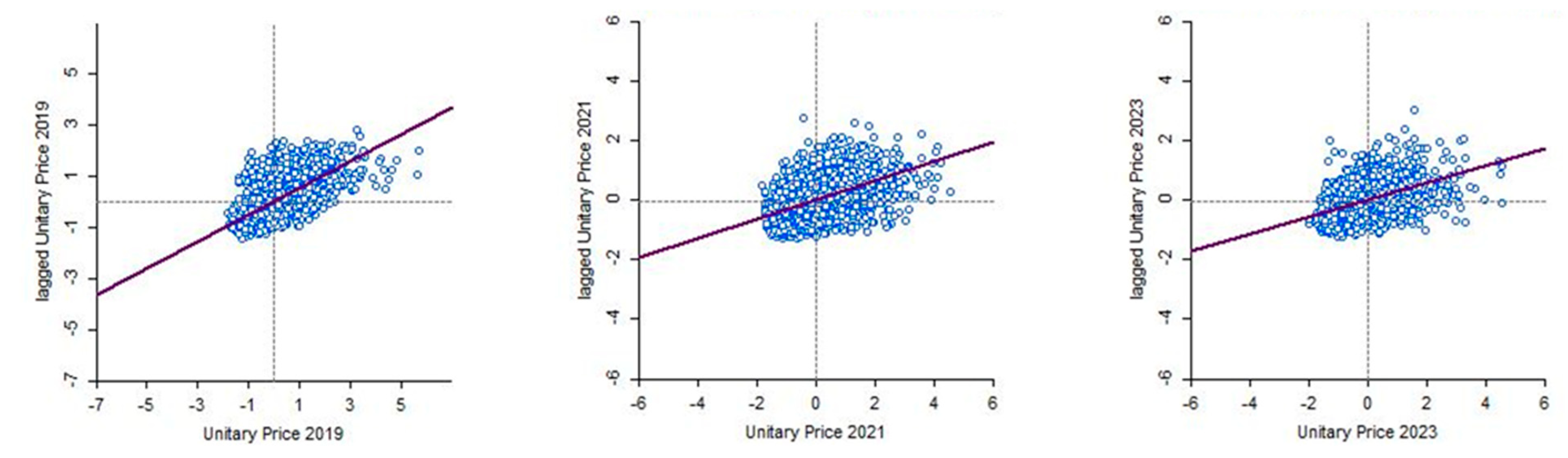
7. A Spatial and Econometric Analysis

7.1. The Multivariate Regressions

Before performing the MR, it is necessary to verify whether the feature selection process has ensured the minimum balance between the number of observations in every DBs and the number of used independent variables. Several “rules-of-thumb” have been suggested in the literature over time in order to determine the minimum number of observations necessary to elaborate a multiple regression analysis. In [82], the authors suggest that N ≥ 50 + 8R in multiple correlations and N ≥ 104 + R in partial correlations, where N is the number of minimum observations, and R is the number of predictors. However, the authors in [82] also state that for multiple correlations, the rule N ≥ 50 + 8R produces values excessively large for N when R ≥ 7. Therefore, the so-called “effect size” should also be considered in questioning the minimum sample size.
In this case, the number of observations fully justifies the number of the selected regressors later illustrated in this paragraph.
The MR helps to understand the relationships with multiple independent variables, as it is in this research. The dependent variable (Y), i.e., the market value of the property, depends on several independent variables (Xr), namely, the descriptive building features, and R is the total number of the regressors, as in Equation (1):
Y =   a 0 +   β 1 X 1   + +   β r X r   + +   β R X R   ± φ
In the equation:
  • Y is the dependent variable (i.e., the market value measured in €/sqm);
  • a0 is the constant;
  • βr are the coefficients of the regressors Xr, 1 ≤ r ≤ R;
  • Xr are the dependent variables 1 ≤ r ≤ R (i.e., the characteristics of the buildings);
  • R is the total number of dependent variables (Xr);
  • 𝜑 is the error.
The regressors are normalized in the interval 0–1 to be homogeneous and coherent. The normalization allows all the terms to be compared through the same seize order and to be consistent in the results.
With the help of the SPSS 29 software, the authors conduct a stepwise analysis, both forward and backwards, to identify the optimal function that explains the dependent variable. The stepwise analysis includes and excludes iteratively the regressors intending to minimize the error on the forecast. The final regressors are defined as follows:
  • X1 = Building internal services (Ʃ 0/1 of lift, private garden, private garage, shared parking space, cellar, terrace, building automation, central heating, photovoltaic system, MCV, air conditioning, optical fibre, and fireplace);
  • X2 = Floor area (sqm);
  • X3 = Energy class (from 10 to 1, where 10 represents the highest class A4, and 1 the lowest, i.e., class G);
  • X4 = City centre straight line distance (km);
  • X5 = Urban amenities and leisure (total n. of services in 1 km ring buffer of cultural facilities, museums, art galleries, theatres, cinemas, and libraries);
  • X6 = Commercial services (total n. of services in 1 km ring buffer of big shopping malls, big commercial facilities, and small supermarkets);
  • X7 = Bus and tram stop (total n. of services in the Ped shed of bus stop and tram stop).
The MR developed on DB2019 produces the function Y2019, on DB2021 the function is called Y2021, whereas on DB2023 the regression formula is named Y2023. The results of the MR analysis are reported below in Equations (2)–(4). All the regressors show a T-student value > 2 and a p-value < 0.05. The Gaussian distribution of the values representing the difference between the expected value and the forecast can be appreciated by the analysis of residuals. As far as R-sq is concerned, Rsq2019 = 0.71, Rsq2021 = 0.79, and Rsq2023 = 0.74.
Y 2019 = 1766.16 33.29 X 1   0.57 X 2   +   68.88 X 3   25.98 X 4   + 2.65 X 5   17.75 X 6   + 5.14 X 7  
Y 2021 = 1801.46 + 52.31 X 1   6.26 X 2   + 74.59 X 3   92.83 X 4   + 8.92 X 5   9.89 X 6   27.49 X 7
Y 2023 = 1673.95 + 10.62 X 1   2.08 X 2   + 144.07 X 3   57.79 X 4   + 12.94 X 5   29.38 X 6   27.11 X 7
In these equations, X1, X2, and X3 represent the construction properties of the buildings, while X4, X5, X6, and X7 embody location attributes. Since such neighbourhood features add spatial information to the regression analysis, the authors believe that further clarification and exploration of this issue may be required here.
There are fundamental differences between spatial and a-spatial data: unlike the former, the latter usually fulfils certain critical assumptions in statistical analyses [4]. The first assumption is independence within the sample. The assumption of independence underlies not only various techniques, including regression, but, more generally, inference and inferential statistics. However, spatial data tend to violate it because they are characterised by spatial dependence naturally.
The second assumption is spatial homogeneity, which is similar to the first assumption because both properties are related to the covariance of spatial processes, producing similar effects on statistical and inferential analyses.
A regression analysis, as in this research paper, rests on a number of statistical assumptions that, when fulfilled, guarantee the optimal properties of the forecasts. However, it is rare for spatial data to satisfy those assumptions, which implies that, generally, the calculation of model parameters from spatial data samples is carried out in violation of those assumptions, so that regression, including spatial data, tends to be affected by more significant variability than those obtained from a-spatial data. The R-sq calculated in the three models is, in fact, representative of about 70% of the sample, which is good reliability on the forecasts but not optimal, remembering that spatial econometrics naturally deals with spatial dependence and spatial heterogeneity [83].
The crucial point is related to spatial autocorrelation, which measures, regarding a single variable, the correlation (positive or negative) between specific spatial units and other spatial units and the dependence between them [84]. There are several indices of spatial autocorrelation, the best known of which are Moran’s and Geary’s [4].
According to Moran’s index, autocorrelation is positive when neighbouring attributes are more similar (attraction), negative when they are more dissimilar (repulsion), or close to zero when there is no relationship between similarity and distance, in which case the spatial process is a random process (complete spatial randomness) [85]. The Univariate Moran (I) index has been assessed on DB2019, DB2021, and DB2023. According to the following Formula (5):
I = N   i j W ij   i j W ij X i   X med   X j   X med   i j W ij i X i   X med   2
  • 1 ≤ i ≤ N
  • 1 ≤ j ≤ N
  • −1 ≤ I ≤ 1
where N is the number of observations (points in the space), Xi is the variable that describes the phenomena, Xmed is the sample mean, and Wij is the weights matrix. The spatial weights matrix consists of as many elements as spatial units sampled (N), and each of its elements defines the contiguity between two spatial units. Typically, the matrix comprises a binary structure multiplied by a distance friction function. The task of the binary structure is to determine which units are considered contiguous. The matrix obtained by multiplying the binary structure by the distance friction function weighs the observed interaction for the distance between two spatial units in all cases where they are defined as contiguous.
For this reason, the contiguity matrix is often also called the spatial weights matrix. In this case, the spatial observations are points (latitude and longitude). Therefore, the weights matrix is built using the k-nearest neighbour methodology. As such, I2019 = 0.53, I2021 = 0.32, and I2023 = 0.29, also represented in Figure 5.

7.2. Discussing Fluctuations in Market Preferences

By comparing the functions above, i.e., Y2019, Y2021, and Y2023, it is clear that some changes have occurred in the marginal appreciation that buyers attribute to the characteristics of the buildings. Moreover, the RF feature importance process helps to understand the different willingness to pay for specific attributes over time (please refer to Table 7 in Section 6), and the Moran I indexes lead to understanding the evolution of spatial autocorrelation.
Regarding the construction features of the buildings, expressed by the regressors X1, X2, and X3, a higher appreciation of certain features, such as a wider surface area or the energy class, is clearly recorded after the COVID-19 pandemic. The energy class coefficient in the MR is positively correlated to the forecast, and the coefficients increase from 2019 to 2023. In addition, the RF results show the increasing importance of the buildings’ construction characteristics over time.
These results can be considered consistent with similar research performed in other Italian cities, such as in [86], and they can be interpreted as a response to the COVID-19 pandemic: The lockdown periods have changed the way people experience their home and have (obviously) increased the amount of time spent there. Although lockdown periods have now ended, people’s daily routines still remain affected by that experience, as it is, for instance, for smart working new schedules. This made certain features of the houses more significant, like bigger spaces, while technologies and installations are now more appealing to buyers, especially from an energy efficiency point of view. It is significant to mention in this context that the attention to the reduction in energy consumption has also increased with the “110%-Superbonus” and “Sismabonsus” Italian Government initiatives and concomitantly, due to the exponential growth of energy prices and construction costs due to the War in Ukraine [87]. These government initiatives have undoubtedly played an important role in the market value variations according to maintenance characteristics and energy classes. The effects on the real estate market of such initiatives have had additional and simultaneous effects on COVID-19. On the one hand, the demand for properties in poor maintenance conditions was increased, considering that the owner could have benefited from retrofit/renovation bonuses. Furthermore, the demand for energy-efficient performances and good conservation conditions may have been losing some appeal due to the possibility of asking for financial incentives.
Due to the War in Ukraine, however, there has been a significant increase in energy prices, and the request for properties with high energy performances, with new technologies and renewable energy installations, has also increased. Meanwhile, a sharp increase in construction costs has been holding back the construction of new buildings, making the supply of such goods scarce.
Regarding localisation features, the feature importance analysis helps to quantify the impact of the localisation variables on the market price.
First, the proximity to the city centre generally produces a non-linear increase in market values. In this case, the proximity to the city centre clearly shows decreasing RF coefficients from 2019 to 2023. This positional characteristic is prone to influence the market value less after the COVID-19 and Ukraine War events. However, the regression equations still show that the nearer to the centre, the higher the value. Clearly, the city centre’s concentration of services and facilities is the highest, therefore playing a significant role in enhancing people’s quality of life. The main cultural amenities are located in the city centre, and various studies showed that the proximity to an important museum [88], an archaeological site, a historical building [89], or cultural heritage [90] might increase the market values of the properties because of the positive impact on the district’s image [91]. The Moran I index still confirms that as much as the position of the building with respect to the city centre remains determining, the market segmentation (spatial autocorrelation of market prices) has decreased from 2019 to 2023.
The market value is also influenced by accessibility to public transport, and coherently with the analysis developed here, the authors in [92] identified a significant impact of accessibility on market segmentation. However, in this case, the RF analysis also allows us to understand that access to transport has seen a decrease in its impact on the market value from 2021 to 2023.
The proximity of hospitals and medical centres seems to slightly influence the market value in Padova, and such regressors have been excluded from the MRs as they did not show sufficient statistically significance in the regression stepwise analysis. Several researchers have extensively explored this issue in the literature, but their findings produced controversial results. Some authors have found that the proximity to hospitals has a slightly negative impact on the prices, as in [93] and [94], especially if the premise is very close to the hospital [95], probably due to ambulances’ high noise and traffic congestion. However, the same authors [95] have highlighted that medical facilities can increase the market value within a certain distance from the premises (a ring buffer of 1 to 2 miles). Other publications have found no significant impact of hospitals’ proximity on the prices [96].
Educational facilities are slightly correlated to the market value of a property in Padova, and these regressors have been excluded from the MRs since they are not statistically significant enough according to the regression stepwise analysis. The results in the literature are divergent. For instance, in [97,98], the authors have identified a positive impact of educational facilities’ proximity on house prices and the increase in price is often associated with the school rating/performance index. Higher school quality increases housing prices [99], and public high-performing schools seem to have the highest impact [100]. Educational facilities also increase the number of operators in the market demand [101].
Regarding sports facilities and urban parks, the influence on the market value over time in Padova seems negligible in the MRs. The RF coefficients show an increase in impact on the forecast in 2021 and a decrease in importance in 2023. As also mentioned in the literature, as in [102,103,104,105], only large stadiums and arenas produce a sensible variation in market prices, and the results are quite controversial. The effects of proximity to large sports infrastructures lead to a general increase in the prices of the district, but, at the same time, they lead to a decrease in market values of the nearest buildings due to the negative externalities. The literature is relatively consistent in relating an increase in housing prices when a park or a greenway is in the proximity of the building [106] since the quality of the neighbourhood is positively enhanced, especially if inside the “Ped shed” [107].
Commercial facilities show a negative impact in the regression equations produced, even though the RF shows that this is certainly not the primary influence on the prices. These results are quite controversial in the research: In [108], the author detected a rise in housing prices within a proximity range of 1–5 miles. A price increase in the district was also identified by [109] due to the presence of groceries. Big supermarket chains also contribute to a rise in prices, as in [110,111], especially when they are in the Pedestrian Shed [112]. Other studies have found a counter-trend, where the closest houses to commercial facilities may experience a slight decrease in market values due to noise and traffic [113].

8. Discussion and Conclusions

The scope of this study was to highlight the different marginal appreciation of construction and localisation features of properties in determining their market value. The analysis was diachronic and regarded as one exemplary case study in North Italy. The case study has been analysed at three different time points:
  • Before the first COVID-19 pandemic alert;
  • Two years after the first COVID-19 alert but before the outbreak of the War in Ukraine;
  • One year after the outbreak of the War in Ukraine.
Several techniques have been integrated into this research: computer programming in Python language, spatial analysis, Multivariate Regression, and Random Forest feature importance analysis.
First, an automated procedure was developed in Python® computer language to download descriptive data about the buildings. Then, a web-crawling software was produced to extract information from specific real-estate-selling websites. Finally, the set of construction and localisation descriptive features of the buildings to be downloaded was defined.
Specifically, the web crawler was applied at three different time points. The first download dates back to the beginning of the II semester of 2019, to capture a pre-COVID-19 scenario. The second download is dated 2021, the beginning of the II semester, to portray the situation two years after the first COVID-19 alert but before the outbreak of the War. Finally, the third download goes back to the beginning of the I semester in 2023 so as to depict market variations one year after the outbreak of the War in Ukraine.
Before producing the regression models, feature importance and feature selection analyses were applied to the three databases.
The feature selection procedure was chosen to understand the variables’ importance in the Random Forest regressor. This analysis helps to exclude the less significant predictors from the regression models, reducing the complexity and computational time of the regressions.
Then, three forecasting econometric models are produced as Multivariate Regressions to forecast the market value of a property as a function of a bundle of its descriptive characteristics.
The three models are diachronic and are dated 2019, 2121, and 2023. By comparing the three equations, it is possible to understand how the marginal contributions have changed per building feature after those two anomalous events. Particular attention has been dedicated to the comparison of neighbourhood versus construction characteristics.
The significant result of this research is a deep monitoring of the fluctuation in demand preferences in response to the last year’s anomalous events. Location is the primary factor in determining market prices, but other building attributes affect the buyer’s choices more and more. Among the significant limitations of this study, it can be stated that the case study is very specific. The case study of the city of Padova was selected due to the availability of extensive and detailed amount of data from several previous works. However, in further developments of this research, the authors intend to expand this market value analysis methodology to other Italian cities. Another limitation of the present study is the short time span during which the analysis was carried out. For this reason, the authors continue to monitor market variations over time in order to observe diachronic changes and understand future developments.

Author Contributions

Conceptualisation, L.G., A.G.R. and M.S.; formal analysis, A.G.R. and M.S.; methodology, L.G., A.G.R. and M.S.; software, M.S.; supervision, L.G.; validation, A.G.R. and M.S.; writing—original draft, A.G.R.; writing—review and editing, L.G. and A.G.R. All authors have read and agreed to the published version of the manuscript.

Funding

This research received no external funding.

Conflicts of Interest

The authors declare no conflict of interest.

Nomenclature

ao constant (intercept of the regression)
DB database
DB2019 database dated 2019, II semester
DB2021 database dated 2021, II semester
DB2023 database dated 2023, I semester
DBs databases
GIS geographic information system
IUnivariate Moran I index
I2019 Moran I index developed on DB2019
I2021 Moran I index developed on DB2021
I2023 Moran I index developed on DB2023
MR Multivariate Regression
MR2019 Multivariate Regression developed on DB2019
MR2021 Multivariate Regression developed on DB2021
MR2023 Multivariate Regression developed on DB2023
MRs Multivariate Regressions
N number of observations
POIPoint of Interest
POIsPoints of Interest
R total number of predictors
RF Random Forest
U.o.M.unit of measure
Wij the weights matrix
Xi the variable that describe the phenomena
Xmed the sample mean
Xr dependent variables 1 ≤ r ≤ R (i.e., the characteristics of the buildings)
Y dependent variable (i.e., the market value)
Y2019 dependent variable (i.e., the market value 2019)
Y2021 dependent variable (i.e., the market value 2021)
Y2023 dependent variable (i.e., the market value 2023)
βr coefficients of the regressors Xr, 1 ≤ r ≤ R
𝜑 error

References

  1. Safire, W. Location, Location, Location. Available online: https://www.nytimes.com/2009/06/28/magazine/28FOB-onlanguage-t.html (accessed on 30 April 2023).
  2. Wang, A.; Xu, Y. Multiple linear regression analysis of real estate price. In Proceedings of the International Conference on Robots and Intelligent System, ICRIS 2018, Changsha, China, 26–27 May 2018; IEEE: Piscataway, NJ, USA; pp. 564–568. [Google Scholar]
  3. Feng, J.; Zhu, J. Nonlinear regression model and option analysis of real estate price. Dalian Ligong Daxue Xuebao/J. Dalian Univ. Technol. 2017, 57, 545–550. [Google Scholar] [CrossRef]
  4. Bertazzon, S. L’ Analisi Spaziale. La Geografia Che … Conta; FrancoAngeli: Milan, Italy, 2022; ISBN 9788835139461. [Google Scholar]
  5. Simonotti, M. Metodi di Stima Immobiliare; Flaccovio: Palermo, Italy, 2006. [Google Scholar]
  6. Shen, K. Application of market comparison approach in land price appraisal. In Proceedings of the Geology Resource Management and Sustainable Development—Academic Conference Proceedings of 2009 Geology Resource Management and Sustainable Development, CGRMSD 2009, Lushan, China, 30 November 2009; pp. 225–230. [Google Scholar]
  7. Salvo, F.; Tavano, D.; De Ruggiero, M. Hedonic price of the built-up area appraisal in the market comparison approach. Smart Innov. Syst. Technol. 2021, 2, 696–704. [Google Scholar]
  8. D’Amato, M.; Cvorovich, V.; Amoruso, P. Short tab market comparison approach. An application to the residential real estate market in Bari. Stud. Syst. Decis. Control 2017, 86, 401–410. [Google Scholar]
  9. Valier, A. Who performs better? AVMs vs. hedonic models. J. Prop. Investig. Financ. 2020, 38, 213–225. [Google Scholar] [CrossRef]
  10. IAAO Standard on Mass Appraisal of Real Property; International Association of Assessing Officers: Kansas City, MO, USA, 2017.
  11. Štubňová, M.; Urbaníková, M.; Hudáková, J.; Papcunová, V. Estimation of residential property market price: Comparison of artificial neural networks and hedonic pricing model. Emerg. Sci. J. 2020, 4, 530–538. [Google Scholar] [CrossRef]
  12. Amrutphale, J.; Rathore, P.; Malviya, V. A Novel Approach for Stock Market Price Prediction Based on Polynomial Linear Regression. Lect. Notes Netw. Syst. 2020, 100, 161–171. [Google Scholar] [CrossRef]
  13. Pérez-Rave, J.I.; Correa-Morales, J.C.; González-Echavarría, F. A machine learning approach to big data regression analysis of real estate prices for inferential and predictive purposes. J. Prop. Res. 2019, 36, 59–96. [Google Scholar] [CrossRef]
  14. Baldominos, A.; Blanco, I.; Moreno, A.J.; Iturrarte, R.; Bernárdez, Ó.; Afonso, C. Identifying real estate opportunities using machine learning. Appl. Sci. 2018, 8, 2321. [Google Scholar] [CrossRef] [Green Version]
  15. Gabrielli, L.; Ruggeri, A.G. Developing a model for energy retrofit in large building portfolios: Energy assessment, optimization and uncertainty. Energy Build. 2019, 202, 109356. [Google Scholar] [CrossRef]
  16. Gabrielli, L.; Ruggeri, A.G. Optimal design in energy retrofit interventions on building stocks: A decision support system. Green Energy Technol. 2021, 231–248. [Google Scholar]
  17. Pittarello, M.; Scarpa, M.; Ruggeri, A.G.; Gabrielli, L.; Schibuola, L. Artificial neural networks to optimize zero energy building (Zeb) projects from the early design stages. Appl. Sci. 2021, 11, 5377. [Google Scholar] [CrossRef]
  18. Gabrielli, L.; Ruggeri, A.G.; Scarpa, M. Automatic energy demand assessment in low-carbon investments: A neural network approach for building portfolios. J. Eur. Real Estate Res. 2020, 13, 357–385. [Google Scholar] [CrossRef]
  19. Rosen, S. Hedonic prices and implicit markets: Product differentiation in pure competition. J. Polit. Econ. 1974, 82, 34–55. [Google Scholar] [CrossRef]
  20. Del Giudice, V.; De Paola, P.; Torrieri, F.; Pagliara, F.; Nijkamp, P. Estimo e Valutazione Economica dei Progetti: Profili Metodologici ed Applicazioni al Settore Immobiliare; SCIENZE REGIONALI; Il Mulino: Bologna, Italy, 2022; ISBN 9788899306038. [Google Scholar]
  21. Gabrielli, L.; Ruggeri, A.G.; Scarpa, M. How COVID-19 Pandemic Has Affected the Market Value According to Multi-parametric Methods. Lect. Notes Networks Syst. 2022, 482, 1018–1027. [Google Scholar]
  22. Gabrielli, L.; Ruggeri, A.G.; Scarpa, M. Using Artificial Neural Networks to Uncover Real Estate Market Transparency: The Market Value. In Proceedings of the Lecture Notes in Computer Science; Gervasi, O., Murgante, B., Misra, S., Garau, C., Blečić, I., Taniar, D., Apduhan, B.O., Rocha, A.M.A.C., Tarantino, E., Torre, C.M., Eds.; Springer International Publishing: Berlin/Heidelberg, Germany, 2021; Volume 12954 LNCS, pp. 183–192. [Google Scholar]
  23. World Health Organization. Available online: https://www.who.int/ (accessed on 15 October 2021).
  24. Nicola, M.; Alsafi, Z.; Sohrabi, C.; Kerwan, A.; Al-Jabir, A.; Iosifidis, C.; Agha, M.; Agha, R. The socio-economic implications of the coronavirus pandemic (COVID-19): A review. Int. J. Surg. 2020, 78, 185–193. [Google Scholar] [CrossRef]
  25. ANSA Ucraina: La Cronaca, Dall’attacco Alla Chiamata Alle Armi. Alle 4:13 la Notizia di Esplosioni a Kiev, Poi in Rapida Sequenza in Altre Città. Available online: https://www.ansa.it/sito/notizie/mondo/2022/02/24/ucraina-la-cronaca-dallattacco-alla-grande-fuga_3bba3244-a42c-4210-8d41-83c584236fa8.html (accessed on 30 March 2023).
  26. Markus, S. Long-term business implications of Russia’s war in Ukraine. Asian Bus. Manag. 2022, 21, 483–487. [Google Scholar] [CrossRef]
  27. Zahra, S.A. Institutional Change and International Entrepreneurship after the War in Ukraine. Br. J. Manag. 2022, 33, 1689–1693. [Google Scholar] [CrossRef]
  28. Wang, Y.; Bouri, E.; Fareed, Z.; Dai, Y. Geopolitical risk and the systemic risk in the commodity markets under the war in Ukraine. Financ. Res. Lett. 2022, 49, 103066. [Google Scholar] [CrossRef]
  29. Steffen, B.; Patt, A. A historical turning point? Early evidence on how the Russia-Ukraine war changes public support for clean energy policies. Energy Res. Soc. Sci. 2022, 91, 102758. [Google Scholar] [CrossRef]
  30. Rawtani, D.; Gupta, G.; Khatri, N.; Rao, P.K.; Hussain, C.M. Environmental damages due to war in Ukraine: A perspective. Sci. Total Environ. 2022, 850, 157932. [Google Scholar] [CrossRef]
  31. Zhou, X.-Y.; Lu, G.; Xu, Z.; Yan, X.; Khu, S.-T.; Yang, J.; Zhao, J. Influence of Russia-Ukraine War on the Global Energy and Food Security. Resour. Conserv. Recycl. 2023, 188, 106657. [Google Scholar] [CrossRef]
  32. Piech, K. Health Care Financing and Economic Performance during the Coronavirus Pandemic, the War in Ukraine and the Energy Transition Attempt. Sustainability 2022, 14, 10601. [Google Scholar] [CrossRef]
  33. Elvevåg, B.; DeLisi, L.E. The mental health consequences on children of the war in Ukraine: A commentary. Psychiatry Res. 2022, 317, 114798. [Google Scholar] [CrossRef] [PubMed]
  34. Kalaitzaki, A.E.; Tamiolaki, A. Russia-Ukraine War: Jeopardizing the mental health gains already been obtained globally. Asian J. Psychiatr. 2022, 78, 103285. [Google Scholar] [CrossRef]
  35. Quaglio, C.; Todella, E.; Lami, I.M. Adequate Housing and COVID-19: Assessing the Potential for Value Creation through the Project. Sustainability 2021, 13, 10563. [Google Scholar] [CrossRef]
  36. Tokazhanov, G.; Tleuken, A.; Guney, M.; Turkyilmaz, A.; Karaca, F. How is COVID-19 Experience Transforming Sustainability Requirements of Residential Buildings? A Review. Sustainability 2020, 12, 8732. [Google Scholar] [CrossRef]
  37. Tucci, F. Pandemia e Green City. Le necessità di un confronto per una riflessione sul futuro del nostro Abitare. In Pandemia e Alcune Sfide Green del Nostro Tempo; Fondazione Sviluppo Sostenibile: Rome, Italy, 2020. [Google Scholar]
  38. De Toro, P.; Nocca, F.; Buglione, F. Real Estate Market Responses to the COVID-19 Crisis: Which Prospects for the Metropolitan Area of Naples (Italy)? Urban Sci. 2021, 5, 23. [Google Scholar] [CrossRef]
  39. Martinho, V.J.P.D. Impacts of the COVID-19 Pandemic and the Russia–Ukraine Conflict on Land Use across the World. Land 2022, 11, 1614. [Google Scholar] [CrossRef]
  40. Trojanek, R.; Gluszak, M. Short-run impact of the Ukrainian refugee crisis on the housing market in Poland. Financ. Res. Lett. 2022, 50, 103236. [Google Scholar] [CrossRef]
  41. Belasen, A.R.; Polachek, S.W. How disasters affect local labor markets: The effects of hurricanes in Florida. J. Hum. Resour. 2009, 44, 251–276. [Google Scholar] [CrossRef]
  42. Boustan, L.P.; Kahn, M.E.; Rhode, P.W.; Yanguas, M.L. The effect of natural disasters on economic activity in US counties: A century of data. J. Urban Econ. 2020, 118, 103257. [Google Scholar] [CrossRef]
  43. Yakub, A.A.; Hishamuddin, M.A.; Kamalahasan, A.; Abdul Jalil, R.B.; Salawu, A.O. An Integrated Approach Based on Artificial Intelligence Using Anfis and Ann for Multiple Criteria Real Estate Price Prediction. Plan. Malays. 2021, 19, 270–282. [Google Scholar] [CrossRef]
  44. Kalliola, J.; Kapočiūte-Dzikiene, J.; Damaševičius, R. Neural network hyperparameter optimization for prediction of real estate prices in Helsinki. PeerJ Comput. Sci. 2021, 7, e444. [Google Scholar] [CrossRef] [PubMed]
  45. Quotazioni Immobiliari nel Comune di Padova. Available online: https://www.immobiliare.it/mercato-immobiliare/veneto/padova/ (accessed on 30 March 2023).
  46. Nomisma Spa—Servizi di Analisi e Valutazioni Immobiliari. Available online: https://www.nomisma.it/servizi/osservatori/osservatori-di-mercato/osservatorio-immobiliare/ (accessed on 30 March 2023).
  47. Agenzia delle Entrate—Osservatorio del Mercato Immobiliare. Available online: https://www.pd.camcom.it/gestisci-impresa/studi-informazione-economica/quotazioni-immobili-1 (accessed on 30 March 2023).
  48. Sirmans, G.S.; Macpherson, A.D.; Zietz, N.E. The Composition of Hedonic Pricing Models. J. Real Estate Lit. 2005, 13, 3–43. [Google Scholar] [CrossRef]
  49. Mora-Garcia, R.T.; Cespedes-Lopez, M.F.; Perez-Sanchez, V.R.; Marti, P.; Perez-Sanchez, J.C. Determinants of the price of housing in the province of Alicante (Spain): Analysis using quantile regression. Sustainability 2019, 11, 437. [Google Scholar] [CrossRef] [Green Version]
  50. Wolf, L.; Murray, A. Spatial Analysis. In International Encyclopedia of Geography. People, the Earth, Environment and Technology; Wiley: New York, NY, USA, 2016. [Google Scholar]
  51. Brueckner, J.K.; Thisse, J.F.; Zenou, Y. Why is central Paris rich and downtown Detroit poor? An amenity-based theory. Eur. Econ. Rev. 1999, 43, 91–107. [Google Scholar] [CrossRef]
  52. Dubé, J.; Thériault, M.; Des Rosiers, F. Commuter rail accessibility and house values: The case of the Montreal South Shore, Canada, 1992–2009. Transp. Res. Part A Policy Pract. 2013, 54, 49–66. [Google Scholar] [CrossRef]
  53. Lin, J.J.; Hwang, C.H. Analysis of property prices before and after the opening of the Taipei subway system. Ann. Reg. Sci. 2004, 38, 687–704. [Google Scholar] [CrossRef]
  54. Zhang, B.; Li, W.; Lownes, N.; Zhang, C. Estimating the impacts of proximity to public transportation on residential property values: An empirical analysis for hartford and stamford areas, connecticut. ISPRS Int. J. Geo-Inf. 2021, 10, 44. [Google Scholar] [CrossRef]
  55. Lin, C.W.; Wang, J.C.; Zhong, B.Y.; Jiang, J.A.; Wu, Y.F.; Leu, S.W.; Nee, T.E. Lie symmetry analysis of the effects of urban infrastructures on residential property values. PLoS ONE 2021, 16, e0255233. [Google Scholar] [CrossRef]
  56. Filippova, O.; Sheng, M. Impact of bus rapid transit on residential property prices in Auckland, New Zealand. J. Transp. Geogr. 2020, 86, 102780. [Google Scholar] [CrossRef]
  57. Ryan, S. Property values and transportation facilities: Finding the transportation-land use connection. J. Plan. Lit. 1999, 13, 412–427. [Google Scholar] [CrossRef]
  58. Zhang, D.; Jiao, J. How does urban rail transit influence residential property values? Evidence from an emerging Chinese megacity. Sustainability 2019, 11, 534. [Google Scholar] [CrossRef] [Green Version]
  59. Cavallaro, F.; Bruzzone, F.; Nocera, S. Spatial and social equity implications for High-Speed Railway lines in Northern Italy. Transp. Res. Part A Policy Pract. 2020, 135, 327–340. [Google Scholar] [CrossRef]
  60. Beenstock, M.; Feldman, D.; Felsenstein, D. Hedonic pricing when housing is endogenous: The value of access to the trans-Israel highway. J. Reg. Sci. 2016, 56, 134–155. [Google Scholar] [CrossRef] [Green Version]
  61. Cordera, R.; Coppola, P.; dell’Olio, L.; Ibeas, Á. The impact of accessibility by public transport on real estate values: A comparison between the cities of Rome and Santander. Transp. Res. Part A Policy Pract. 2019, 125, 308–319. [Google Scholar] [CrossRef]
  62. Pan, H.; Zhang, M. Rail transit impacts on land use: Evidence from Shanghai, China. Transp. Res. Rec. 2008, 2048, 16–25. [Google Scholar] [CrossRef]
  63. Boshoff, D.G.B. The influence of rapid rail systems on office values: A case study on South Africa. Pac. Rim Prop. Res. J. 2017, 23, 267–302. [Google Scholar] [CrossRef]
  64. Zhong, H.; Li, W. Rail transit investment and property values: An old tale retold. Transp. Policy 2016, 51, 33–48. [Google Scholar] [CrossRef]
  65. Ibeas, Á.; Cordera, R.; Dell’Olio, L.; Coppola, P.; Dominguez, A. Modelling transport and real-estate values interactions in urban systems. J. Transp. Geogr. 2012, 24, 370–382. [Google Scholar] [CrossRef] [Green Version]
  66. Bohman, H.; Nilsson, D. The impact of regional commuter trains on property values: Price segments and income. J. Transp. Geogr. 2016, 56, 102–109. [Google Scholar] [CrossRef] [Green Version]
  67. Bollinger, C.R.; Ihlanfeldt, K.R.; Bowes, D.R. Spatial Variation in Office Rents within the Atlanta Region. Urban Stud. 1998, 35, 1097–1118. [Google Scholar] [CrossRef]
  68. Landis, J. BART Access and Office Building Performance; University of California: Berkeley, CA, USA, 1995. [Google Scholar]
  69. Zhou, Z.; Chen, H.; Han, L.; Zhang, A. The Effect of a Subway on House Prices: Evidence from Shanghai. Real Estate Econ. 2021, 49, 199–234. [Google Scholar] [CrossRef]
  70. Weinstein, B.L.; Clower, T.L. An Assessment of the DART LRT on Taxable Property Valuations and Transit Oriented Development; University of North Texas: Denton, TX, USA, 2002. [Google Scholar]
  71. Li, S.; Chen, L.; Zhao, P. The impact of metro services on housing prices: A case study from Beijing. Transportation 2017, 46, 1291–1317. [Google Scholar] [CrossRef]
  72. Dai, X.; Bai, X.; Xu, M. The influence of Beijing rail transfer stations on surrounding housing prices. Habitat Int. 2016, 55, 79–88. [Google Scholar] [CrossRef]
  73. Shen, Q.; Xu, S.; Lin, J. Effects of bus transit-oriented development (BTOD) on single-family property value in Seattle metropolitan area. Urban Stud. 2018, 55, 2960–2979. [Google Scholar] [CrossRef]
  74. Lieske, S.N.; van den Nouwelant, R.; Han, J.H.; Pettit, C. A novel hedonic price modelling approach for estimating the impact of transportation infrastructure on property prices. Urban Stud. 2021, 58, 182–202. [Google Scholar] [CrossRef]
  75. Zhang, L.; Zhou, T.; Mao, C. Does the difference in urban public facility allocation cause spatial inequality in housing prices? Evidence from Chongqing, China. Sustainability 2019, 11, 6096. [Google Scholar] [CrossRef] [Green Version]
  76. Tatwani, S.; Kumar, E. Parametric comparison of various feature selection techniques. J. Adv. Res. Dyn. Control Syst. 2019, 11, 1180–1190. [Google Scholar] [CrossRef]
  77. Ghosh, M.; Guha, R.; Sarkar, R.; Abraham, A. A wrapper-filter feature selection technique based on ant colony optimization. Neural Comput. Appl. 2020, 32, 7839–7857. [Google Scholar] [CrossRef]
  78. Suresh, S.M.S.; Narayanan, A. Improving Classification Accuracy Using Combined Filter+Wrapper Feature Selection Technique. In Proceedings of the 2019 3rd IEEE International Conference on Electrical, Computer and Communication Technologies, ICECCT 2019, Tamil Nadu, India, 20–22 February 2019; Department of Computer Science and Engineering, Amrita School of Engineering, Amrita Vishwa Vidyapeetham: Amritapuri, India, 2019. [Google Scholar]
  79. Yassi, M.; Moattar, M.H. Robust and stable feature selection by integrating ranking methods and wrapper technique in genetic data classification. Biochem. Biophys. Res. Commun. 2014, 446, 850–856. [Google Scholar] [CrossRef] [PubMed]
  80. Siham, A.; Sara, S.; Abdellah, A. Feature selection based on machine learning for credit scoring: An evaluation of filter and embedded methods. In Proceedings of the 2021 International Conference on INnovations in Intelligent SysTems and Applications, INISTA 2021—Proceedings, Kocaeli, Turkey, 17 May 2021; Hassan II University of Casablanca, Networks, Telecoms and Multimedia LIM@II-FSTM: Mohammedia, Morocco, 2021. [Google Scholar]
  81. Ugolini, M. Metodologie di Apprendimento Automatico Applicate Alla Generazione di Dati 3D; University of Bologna: Bologna, Italy, 2014; pp. 1–49. [Google Scholar]
  82. Green, S.B. How Many Subjects Does It Take To Do A Regression Analysis. Multivariate Behav. Res. 1991, 26, 499–510. [Google Scholar] [CrossRef] [PubMed]
  83. Anselin, L. Spatial Econometric. Methods and Models; Springer: New York, NY, USA, 1988. [Google Scholar]
  84. Getis, A. Reflections on Spatial Autocorrelation. Reg. Sci. Urban Econ. 2007, 37, 491–496. [Google Scholar] [CrossRef]
  85. Diggle, P.J. On Parameter Estimation and Goodness-of-Fit Testing for Spatial Point Patterns. Biometrics 1979, 35, 87–101. [Google Scholar] [CrossRef]
  86. Tajani, F.; Morano, P.; Di Liddo, F.; Guarini, M.R.; Ranieri, R. The Effects of COVID-19 Pandemic on the Housing Market: A Case Study in Rome (Italy). Lect. Notes Comput. Sci. 2021, 12954, 50–62. [Google Scholar]
  87. Superbonus 110%. Available online: https://www.governo.it/superbonus (accessed on 17 December 2021).
  88. Sheppard, S.C.; Oehler, K.; Benjamin, B.; Kessler, A. Culture and Revitalization: The Economic Effects of MASS MoCA on Its Community; Williams College: Williamstown, MA, USA, 2006. [Google Scholar]
  89. Moro, M.; Mayor, K.; Lyons, S. Does the housing market reflect cultural heritage? A case study of Greater Dublin. Environ. Plan. A 2013, 45, 2884–2903. [Google Scholar] [CrossRef]
  90. Ahlfeldt, G.M.; Maennig, W. Substitutability and complementarity of urban amenities: External effects of built heritage in Berlin. Real Estate Econ. 2010, 38, 285–323. [Google Scholar] [CrossRef]
  91. Moreno Gil, S.; Ritchie, J.R.B. Understanding the museum image formation process: A comparison of residents and tourists. J. Travel Res. 2009, 47, 480–493. [Google Scholar] [CrossRef]
  92. Adair, A.; McGreal, S.; Smyth, A.; Cooper, J.; Ryley, T. House prices and accessibility: The testing of relationships within the Belfast Urban Area. Hous. Stud. 2000, 15, 699–716. [Google Scholar] [CrossRef]
  93. Rivas, R.; Patil, D.; Hristidis, V.; Barr, J.R.; Srinivasan, N. The impact of colleges and hospitals to local real estate markets. J. Big Data 2019, 6, 7. [Google Scholar] [CrossRef]
  94. Tian, G.; Wei, Y.D.; Li, H. Effects of accessibility and environmental health risk on housing prices: A case of Salt Lake County, Utah. Appl. Geogr. 2017, 89, 12–21. [Google Scholar] [CrossRef]
  95. Waddell, P.; Shukla, V. Employment Dynamics, Spatial Restructuring, and the Business Cycle. Geogr. Anal. 1993, 25, 35–52. [Google Scholar] [CrossRef]
  96. Yuan, F.; Wei, Y.D.; Wu, J. Amenity effects of urban facilities on housing prices in China: Accessibility, scarcity, and urban spaces. Cities 2020, 96, 102433. [Google Scholar] [CrossRef]
  97. Gibbons, S.; Machin, S. Paying for Primary Schools: Admission Constraints, School Popularity or Congestion? Econ. J. 2006, 116, 77–92. [Google Scholar] [CrossRef]
  98. Gibbons, S.; Machin, S. Valuing English primary schools. J. Urban Econ. 2003, 53, 197–219. [Google Scholar] [CrossRef] [Green Version]
  99. Wen, H.; Xiao, Y.; Hui, E.C.M.; Zhang, L. Education quality, accessibility, and housing price: Does spatial heterogeneity exist in education capitalization? Habitat Int. 2018, 78, 68–82. [Google Scholar] [CrossRef]
  100. Fack, G.; Grenet, J. When do better schools raise housing prices? Evidence from Paris public and private schools. J. Public Econ. 2010, 94, 59–77. [Google Scholar] [CrossRef] [Green Version]
  101. Owusu-Edusei, K.; Espey, M.; Lin, H. Does Close Count? School Proximity, School Quality, and Residential Property Values. J. Agric. Appl. Econ. 2007, 39, 211–221. [Google Scholar] [CrossRef] [Green Version]
  102. Feng, X.; Humphreys, B.R. The impact of professional sports facilities on housing values: Evidence from census block group data. City Cult. Soc. 2012, 3, 189–200. [Google Scholar] [CrossRef]
  103. Ahlfeldt, G.M.; Kavetsos, G. Form or function? The effect of new sports stadia on property prices in London. J. R. Stat. Soc. Ser. A Stat. Soc. 2014, 177, 169–190. [Google Scholar] [CrossRef] [Green Version]
  104. Ahlfeldt, G.M.; Maennig, W. Impact of sports arenas on land values: Evidence from Berlin. Ann. Reg. Sci. 2010, 44, 205–227. [Google Scholar] [CrossRef] [Green Version]
  105. Tu, C.C. How Does a New Sports Stadium Affect Housing Values? The Case of FedEx Field. Land Econ. 2005, 81, 379–395. [Google Scholar] [CrossRef]
  106. Nicholls, S.; Crompton, J.L. The impact of greenways on property values: Evidence from Austin, Texas. J. Leis. Res. 2005, 37, 321–341. [Google Scholar] [CrossRef]
  107. Smith, D. Valuing Housing and Green Spaces: Understanding Local Amenities, the Built Environment and House Prices in London; University College London: London, UK, 2010; ISBN 9781847813909. [Google Scholar]
  108. Van Fossen, W. The Effect of Supermarket Entrance on Nearby Residential Property Values in the United States from 1997 to 2015; Yale University: New Haven, CT, USA, 2017. [Google Scholar]
  109. Kole, K. Grocery Stores Raise Property Values: Evidence from FRESH; University of California: Irvine, CA, USA, 2021; pp. 1–27. [Google Scholar]
  110. Neill, P.O. Homes Close to a Supermarket Can Boost House Prices by More than £21,000; mpamag: Washington, DC, USA, 2018. [Google Scholar]
  111. Bomberg, M. The Value of Food: The impact of supermarket proximity on home values in Oakland. Policy Matters J. 2012, 5–12. [Google Scholar]
  112. Yang, L.; Wang, B.; Zhou, J.; Wang, X. Walking accessibility and property prices. Transp. Res. Part D Transp. Environ. 2018, 62, 551–562. [Google Scholar] [CrossRef]
  113. Tiemann, L. The Effect of Grocery Store Openings on Residential Property Prices: Evidence from Morrisons Stores in England; University of Groningen: Groningen, The Netherlands, 2020. [Google Scholar]
Figure 1. Workflow and the methodological approach.
Land 12 01248 g001
Figure 2. Historical series of the asking prices in Padova for residential properties in optimal/good/poor conditions (immobiliare.it, data collected at City level).
Land 12 01248 g002
Figure 3. Historical series of the transaction prices in Padova for residential properties in optimal/good/poor conditions (Nomisma, data collected at City level).
Land 12 01248 g003
Figure 4. Collected and geo-localised observations in Padova.
Land 12 01248 g004
Figure 5. Univariate Moran I.
Land 12 01248 g005
Table 1. Average transaction prices in Padova: evolution over time (Nomisma).
Transaction Prices in PADOVA (€/sqm)
Semester, YearMaintenance ConditionsPrestigious AreasCentreSemi-CentreSuburbs
MinMaxMinMaxMinMaxMinMax
I 2022 New constructions 35324290296436591910225412141547
Good maintenance conditions2655322121192579132217399451212
Poor maintenance conditions16322160146217908581180623851
I 2021New constructions 34824209279335181846215911921496
Good maintenance conditions2583303820412496127316859251197
Poor maintenance conditions15732062144217078351140608824
I 2020New constructions 35204323276134401857216812011507
Good maintenance conditions2612317020752524128516649011183
Poor maintenance conditions15712155144017188471154603835
I 2019New constructions 34514226274534851848217512121542
Good maintenance conditions2571310820422583130716729191194
Poor maintenance conditions15772142148317888551147618841
Table 2. Regressors: the construction features.
INTRINSIC FEATURES: Construction Characteristics
Building construction characteristicsTerrace AreaEnergy Class
Floor areaTop FloorConstruction year
no. of bathroomsFireplaceTypology of the building
no. of roomsMaintenance levelApartment
FloorBuilding installationsApartment in a Villa
no. of internal floorsBuilding AutomationPenthouse
Common gardenCentral HeatingFarmhouse
Private GardenPhotovoltaic SystemLoft
Private Garden AreaMechanical VentilationAttic
Private GarageAir ConditioningMulti-storey single-family home
Private Garage AreaOptical FiberSingle-family home
Common Parking SpaceLiftTerraced house
BasementSolar PanelsTwo-family villa
Basement areaHeat PumpMulti-family villa
Terrace
Table 3. Regressors: the neighbourhood features.
EXTRINSIC FEATURES: Neighbourhood and Accessibility
Point of Interest (POI) Point of Interest (POI)
market segmentCity Centre commercial facilitiesShopping malls
central train station Big commercial areas
accessibility to trsnsportsminor train stops Small-supermarkets
Bus stop natural amenitiesUrban Parks
Tram stop Public gardens
education facilitiesnursery modern amenitiesSport facilities
kindergarten Hospitals
primary school Pharmacies
Table 4. Construction features, U.o.M.
INTRINSIC FEATURES: Construction Characteristics
VariableUnitVariableUnitVariableUnit
Floor areasqmTerrace AreasqmEnergy Class10 ->1 (A4 -> G)
no. of bathroomsnumberTop Floor0/1Construction yearYear (number)
no. of roomsnumberBuilding Automation0/1Apartment0/1
FloornumberCentral Heating0/1Apartment in a Villa0/1
no. of internal floorsnumberPhotovoltaic System0/1Penthouse0/1
Common garden0/1Mechanical Ventilation0/1Farmhouse0/1
Private Garden0/1Air Conditioning0/1Loft0/1
Private Garden AreasqmOptical Fiber0/1Attic0/1
Private Garage0/1Lift0/1Multi-storey single-family home0/1
Private Garage AreasqmSolar Panels0/1Single-family home0/1
Common Parking Space0/1Heat Pump0/1Terraced house0/1
Basement0/1Fireplace0/1Two-family villa0/1
Basement areasqmMaintenance level1/2/3/4Multi-family villa0/2
Terrace0/1
Table 5. Neighbourhood features, U.o.M.
EXTRINSIC FEATURES: Localization and Accessibility
VariableUnit
positionLatitude of the building (observation)coordinate
Longitude of the building (observation)coordinate
distanceStraight line distance from POIKm
Actual travel distance from POI by carKm
timeTravel time from POI by carmin
Travel time from POI on footmin
Travel time from POI by public transportsmin
proximityN. of POI in the Ped shed (400 m)n.
N. of POI in a 1 Km ring buffern.
Table 6. Definitive construction features.
INTRINSIC FEATURES: Construction Characteristics
VariableUnitVariableUnitVariableUnit
Building construction characteristicsMaintenance level1/2/3/4Typology of the building
Floor areasqmEnergy Class10 ->1 (A4 -> G)Apartment0/1
no. of bathroomsnumberConstruction yearYear (number)Apartment in a Villa0/1
no. of roomsnumberBuilding InstallationsPenthouse0/1
FloornumberBuilding Automation0/1Farmhouse0/1
no. of internal floorsnumberCentral Heating0/1Loft0/1
Common garden0/1Photovoltaic System0/1Attic0/1
Private Garden0/1Mechanical Ventilation0/1Multi-storey single-family home0/1
Private Garage0/1Air Conditioning0/1Single-family home0/1
Common Parking Space0/1Optical Fiber0/1Terraced house0/1
Basement0/1Lift0/1Two-family villa0/1
Terrace0/1Solar Panels0/1Multi-family villa0/1
Top Floor0/1Heat Pump0/1
Table 7. Random-forest-aggregated coefficients.
Class Element or FunctionRF Coefficients
Intrinsic201920212022
Typology of the building1.24%0.94%0.80%
Building construction characteristics31.49%38.23%74.67%
Building installations2.13%1.53%0.42%
Extrinsic201920212022
City centre proximity35.70%12.88%4.81%
Transports accessibility3.36%3.60%1.80%
Health services proximity4.72%4.40%2.98%
Urban amenities and leisure11.95%28.19%8.73%
Commercial areas3.46%4.61%2.71%
Education facilities proximity5.95%5.61%3.07%
100.00%100.00%100.00%
Disclaimer/Publisher’s Note: The statements, opinions and data contained in all publications are solely those of the individual author(s) and contributor(s) and not of MDPI and/or the editor(s). MDPI and/or the editor(s) disclaim responsibility for any injury to people or property resulting from any ideas, methods, instructions or products referred to in the content.

